Forward Prediction of Runoff Data in Data-Scarce Basins with an Improved Ensemble Empirical Mode Decomposition (EEMD) Model

Abstract

Data scarcity is a common problem in hydrological calculations that often makes water resources planning and engineering design challenging. Combining ensemble empirical mode decomposition (EEMD), a radial basis function (RBF) neural network, and an autoregression (AR) model, an improved EEMD prediction model is proposed for runoff series forward prediction, i.e., runoff series extension. In the improved model, considering the decomposition-prediction-reconstruction principle, EEMD was employed for decomposition and reconstruction and the RBF and AR model were used for component prediction. Also, the method of tracking energy differences (MTED) was used as stopping criteria for EEMD in order to solve the problem of mode mixing that occurs frequently in EEMD. The orthogonality index (Ort) and the relative average deviation (RAD) were introduced to verify the mode mixing and prediction performance. A case study showed that the MTED-based decomposition was significantly better than decomposition methods using the standard deviation (SD) criteria and the G. Rilling (GR) criteria. After MTED-based decomposition, mode mixing in EEMD was suppressed effectively (|Ort| < 0.23) and stable orthogonal components were obtained. For this, annual runoff series forward predictions using the improved EEMD-based prediction model were significantly better (RAD < 11.1%) than predictions by the rainfall-runoff method and the AR model method. Thus, this forward prediction model can be regarded as an approach for hydrological series extension, and shows promise for practical applications.

1. Introduction

Hydrological data scarcity is a constant challenge for international hydrological research. In 2003, the International Association of Hydrological Sciences (IAHS) launched an initiative called “predictions in ungauged basins (PUB)” for the IAHS Decade at the 23rd International Union of Geodesy and Geophysics (IUGG) in Sapporo, Japan. This initiative strongly promoted the development of hydrological research in ungauged basins [1]. In 2013, a new science decade of IAHS was approved, “Panta Rhei—Everything Flows”, which made global hydrological researchers aware of the slow progress in developing innovative hydrological research methods to solve the problem of hydrological data scarcity [2]. It is well known that runoff data are the most important hydrological data for river-basin management and are fundamental to hydraulic engineering design and water-resource management. If a catchment has few or no runoff data, then it is difficult to carry out policies and strategies in water-resource management. Therefore, it is important to develop innovative methods to address the problem of runoff data scarcity to service global hydrological research and engineering design.

To address the scarcity of runoff data, many researchers have proposed various prediction methods. They are generally divided into two major categories: physics-based and data-driven methods. The physics-based methods usually build a proper hydrological model in the few- or no-data catchments according to the catchment condition, and obtain some unknown model parameters directly from other river basins that have observed data. When meteorological data and underlying surface data in the few- or no-data catchments are available, the hydrological processes can be simulated to obtain the runoff data series in the ungauged basins or extend the series in the few-data basins. In recent years, many physics-based methods have been proposed to undertake the predictions in ungauged basins. Servat et al. [3] developed two rainfall-runoff models (GR3 and CREC) which can do runoff prediction from ungauged basins on the basis of land use and rainfall distribution over the year. McIntyre et al. [4] proposed a new approach to the regionalization of conceptual rainfall-runoff models based on ensemble modeling and model averaging. Model parameters were calibrated for 10 gauged basins with hydrological conditions similar to those of the ungauged basins. Also, ensemble predictions of runoff were done for ungauged basins. Wan et al. [5] developed a lumped conceptual rainfall-runoff model for rapid runoff prediction in south Florida with a unique and complicated hydrological setting. Li et al. [6] evaluated two regionalization approaches, spatial proximity and physical similarity, by which two runoff models (SIMHYD and GR4J) were used to predict runoff from the Yarlung Tsangpo River basin. Because these models are based on physical causes, the procedure is very complex and highly susceptible to factors such as the integrity and accuracy of the data on the river basin’s underlying surface conditions, spatial-temporal variance of meteorological data, complexity of rainfall-runoff process, and limited understanding of circulation patterns of water in the basins [7]. In recent years, the precision of predictions by hydrological simulations has been found to be far from satisfactory in some regions, so hybrid models coupling physics-based models with data-driven methods have gained more attention.

Data-driven methods are generally used to make short-term predictions or data extension using mathematical methods and intelligent algorithms via the statistical characteristics of short observational runoff series or unknown meteorological and hydrological black-box models in data-scarce basins or reference watersheds. Besaw et al. [8] developed and tested two artificial neural networks (ANNs) to predict runoff from the Winooski River basin with time-lagged records of precipitation and temperature as input data. Mohamoud [9] employed flow duration curves for forecasting flow in ungauged basins by combining dominant landscape and climate descriptors from 29 nearby catchments with multiple regression. It is well-known that data-driven methods require less data and have a simpler structure than physics-based methods. Furthermore, data-driven methods have a good prediction performance without really simulating the rainfall-runoff process, and can avoid the complex physical process and the influence of model uncertainty. Thus, data-driven methods are usually used as alternative and similar or even superior to those of physics-based methods in ungauged basins where hydrological model simulations cannot be carried out effectively. Nowadays, they have been widely used in hydraulic engineering design. However, they are not universal and are affected by regional conditions. For instance, in north-western China, due to the poor similarity of reference basins and the complicated and changeable rainfall-runoff relationships in the region, rainfall data in the basin and the hydrological characteristics in the reference basin cannot be used as data-driven model inputs in the region. Therefore, the prediction of runoff series in such regions should preferably be based on the existing short runoff data than the unsatisfied rainfall-runoff model or poor similarity of the reference basin. Generally, data extension based on the existing runoff data is called forward prediction, which means predicting a non-measured runoff process before the existing runoff records by data-extension methods.

In the steady state, time-series models and artificial intelligence algorithms, such as artificial neural networks (ANNs) [10,11,12,13,14] and support vector machines (SVMs) [15,16,17,18], can make satisfactory predictions. However, under the dual influence of global climate change and intense human activities in recent years, runoff series have exhibited such characteristics as high complexity, non-stationarity, non-linearity and multiple time-scales [19,20,21]. These characteristics make analysis of runoff characteristics and conventional hydrological time-series forecasting more difficult. The precision of conventional prediction methods does not satisfy the requirements of current engineering design and hydrological research. Therefore, a new prediction method should be developed for hydrological data extension to meet hydraulic engineering design demands.

The multiple time scales of hydrological time series refer to the existence of multi-level time scales and local features in the hydrological series changes in the time domain. For multiple time-scales issues with non-stationarity and non-linearity variables, many time-scale decomposition approaches have been introduced to separate the different time scales in hydrological series for hydrological prediction and to provide important support for system analysis and runoff prediction. For example, the wavelet transform (WT) has been adopted by many researchers for analyzing hydrological time series with multiple scales due to its excellence in situations with multiple resolutions in time and frequency domains [22,23,24,25]. Essentially, a wavelet transform is a Fourier transform with an adjustable window, and the signal should be stable in the WT window. Therefore, it is still susceptible to the limitations of Fourier analysis. Although WT provides high resolution in both the frequency domain and the time domain, certain limitations of this method may generate some false harmonic waves. Thus, the selection of WT basis functions is critical and has a significant impact on the wavelet decomposition performance. In order to promote the development of multiple time-scale analysis approaches, Huang proposed a novel signal analysis method in 1998 called empirical mode decomposition (EMD) [26]. This method is essentially the smoothing treatment of the signal, by which the multi-scale fluctuation or trend components in the signal are decomposed to generate a series of intrinsic mode functions (IMFs) and a residual. Comparing two approaches, it can be seen that an EMD-based Hilbert spectrum and a wavelet spectrum have the same characteristics on the linear framework, while the Hilbert spectrum has significantly higher resolution in both time and frequency domains. Therefore, it is often considered that the EMD result can reflect non-stationary and non-linearity characteristics in the original series more accurately than the WT method, and EMD is regarded as a more effective way to process complex signals. In classical hydrology, a hydrological time series can be regarded as a set of random components, periodical components and trend component. When the decomposition result of the EMD is perfect, the high-frequency components, the low-frequency components and the residual obtained by the decomposition can be approximated as random components, periodic components, and the trend [27,28]. Nowadays, EMD has become a new method for multi-time-scale analysis of non-stationary hydrological time series and has been successfully applied in hydrological research around the world [29,30]. Based on the EMD method, researchers have proposed “decomposition-prediction-reconstruction” coupling models which improve the precision of hydrological prediction effectively [31,32,33]. However, limitations still exist, such as mode mixing and IMFs’ orthogonality effect on the EMD performance and prediction precision. Ideally, each component obtained after the decomposition should contain information on one time scale. However, due to the defects of the decomposition method and the random fluctuations in hydrological series, a component obtained after decomposition may contain different information belonging to other components. That is called mode mixing, which will lead to an unclear physical meaning of each component and confusion in further analysis. The orthogonality of EMD can be understood mathematically in that each IMF decomposed is orthogonal and also can be understood in the decomposing operation in that there is no energy loss of the original series in the process of extracting components in the ideal state. Unfortunately, the total energy of the components is always significantly different from the energy of the original series in the actual EMD process. To address these issues, Wu and Huang proposed the ensemble EMD (EEMD) method to suppress mode mixing in EMD [34,35]. However, EEMD is not perfect, and mode mixing still occurs among low-frequency components. So, it is inferred that a proper stopping criteria is critical for EMD, which can guarantee that the EEMD method can provide satisfactory decomposition results [36]. For hydrological time series, a proper stopping criteria not only improves the precision of fluctuation component extraction in hydrological time-series data, but also preserves the long-range trend in the series to the greatest extent possible, which significantly influences the accuracy of forward prediction. In the EEMD, the stopping criteria is called the SD criteria, in which the standard deviation is used to stop the decomposition procedure [26]. Later, G. Rilling proposed the so-called G. Rilling (GR) criteria [37], which leverages the evaluation function $\sigma (t)$ and the predefined threshold to control when the sifting process stops. In the GR criteria, two conditions are to be fulfilled: the number of extrema and the number of zero-crossings must differ at most by 1, and the mean between the upper and lower envelopes must be close to zero. Compared with the SD criteria proposed by Huang, the GR can obtain the mean value of IMFs more accurately. However, the effects of these criteria are still limited, and the energy loss during sifting and orthogonality among IMFs are not fully addressed. Some problems such as mode mixing cannot still be solved perfectly. To address these issues, Cheng proposed a new EMD sifting stopping criteria, the method of tracking energy differences (MTED), aiming to solve the mode-mixing problem from the perspective of energy. Currently, it has achieved excellent results in fault diagnosis [38].

In view of the above analysis, this paper investigated the applicability of the sifting stopping criteria to hydrological time series. The MTED was selected as the sifting stopping criterion for decomposing runoff series using EEMD. For forward prediction, a radial basis function (RBF) neural network, and an autoregressive (AR) model were combined to create a “decomposition-prediction-reconstruction”-based improved EEMD prediction model in order to predict short runoff series and further solve the problem of runoff data scarcity encountered in hydrological research and engineering design.

2. Materials and Methods

2.1. Empirical Mode Decomposition (EMD)

EMD is a new and innovative self-adaptive time-frequency signal-processing method proposed by Huang in 1998 [29]. This method is primarily designed for non-stationary and non-linear data. Signal decomposition obtains multiple stable IMFs and a monotonic residual based on the data’s own time-scale pattern. In hydrological applications, EMD converts a non-stationary hydrological series into a series of hydrological components with clear patterns that have specific physical meanings [33]. These components are more predictable and can improve the precision of forward prediction significantly. Details of the EMD procedure are as follows:

• Step 1: Identify all local maxima and minima in the original time series X(t). The upper and lower envelopes of the time series are obtained by cubic spline interpolation. The mean of the upper and lower enveloping lines is m(t):

  $$m(t)=\frac{X_{\max }(t)+X_{\min }(t)}{2}$$

  (1)
• Step 2: A new series h(t) is calculated by subtracting the mean m(t) from the original series X(t):

  $$h(t)=X(t)-m(t)$$

  (2)
• Step 3: The EMD sifting stopping criteria determines whether sifting should stop. If the stopping condition is met, h(t) is the IMF, and the next step is executed. If the stopping condition is not met, then h(t) is used as the original series, steps 1 and 2 are repeated until the stopping condition is met, and the first IMF, IMF1 c₁(t), is calculated.
• Step 4: The residual series r₁(t) is obtained by subtracting the IMF c₁(t) from the original series X(t):

  $$r_1(t)=X(t)-c_1(t)$$

  (3)
• Step 5: The residual series r₁(t) is used as the new original series, and steps 1–4 are repeated. All the IMFs, c₁(t), c₂(t), …, c_n(t), are decomposed until c_n(t) is a monotonic or single-extreme-point residual.

2.2. EEMD

The EEMD method is an improvement of EMD method that reduces mode mixing and obtains the actual time-frequency distribution of the signal [35]. The principle is to leverage the statistical features (uniform frequency distribution) of Gaussian white noise. When white noise is added to a signal, the signal becomes continuous on different scales to reduce mode mixing. Details of the decomposition principle and procedure are as follows:

• Step 1: White noise n_i(t) with a mean of 0 and standard deviation constant is added to the original signal X(t) multiple times. The standard deviation of the white noise is set to 0.1–0.4 times the standard deviation of the original signal (0.2 in this study):

  $$X_i(t)=X(t)+n_i(t)$$

  (4)

  where X_i(t) represents the signal after the i-th addition of Gaussian white noise.
• Step 2: Each X_i(t) undergoes the EMD procedure. The IMF component obtained is denoted by c_ij(t), and the residual term is denoted by r_i(t). Among them, c_ij(t) represents the j-th IMF from the decomposition of the signal after the i-th addition of Gaussian white noise.
• Step 3: Steps l and 2 are repeated N times. Based on the principle that the statistical mean of an uncorrelated random series is 0, the IMFs are subjected to an overall averaging operation to eliminate the impact of adding Gaussian white noise to the actual IMF multiple times. Finally, the IMF obtained from EEMD is as follows:

  $$c_j(t)=\frac{1}{N}{\displaystyle \sum _{i=1}^N{c}_{ij}}$$

  (5)

  where c_j(t) represents the j-th IMF of the original signal obtained by EEMD. As the value of N increases, the sum of IMFs for the corresponding white noise approaches 0. At this point, the result of EEMD is as follows:

  $$X(t)={\displaystyle \sum _j{c}_j}(t)+r(t)$$

  (6)

  where r(t) is the final residual, which represents the average trend of the signal. Any signal X(t) can be decomposed into multiple IMFs and one residual via EEMD. IMF c_j(t) (j = 1, 2, …) represents the signal’s components from high frequency to low frequency. Each frequency contains distinct components and varies with the signal X(t).

2.3. Improved Ensemble Empirical Mode Decomposition (EEMD)

Whether the decomposed IMFs are proper or applicable is largely determined by the sifting stopping criteria. Different criteria result in different IMFs from decomposition. Due to the limited applicability of the SD criteria proposed by Huang [34,35] and the GR criteria proposed by G. Rilling [37], the method of tracking energy differences (MTED) is introduced as the sifting stopping criteria to improve the EEMD method.

The MTED is different from the other two sifting stopping criteria. It assumes that the IMFs are finite and orthogonal to each other; that is, in an ideal state, when an IMF is sifted, no energy is lost during sifting. If the EEMD exhibits a smaller energy loss during sifting, it is more likely to guarantee the orthogonality of IMFs and, therefore, the EEMD sifting is more appropriate. It is clear that the MTED mainly works from the perspective of energy and ensures that each extracted IMF and residual are orthogonal in terms of energy. Details of the procedure are as follows [38]:

$$E_{\mathrm{X}}={\displaystyle \underset{-\infty }{\overset{\infty }{\int }}{\left[{\displaystyle \sum _{i=1}^n{c}_i(t)}\right]}^2}dt={\displaystyle \underset{-\infty }{\overset{\infty }{\int }}{c}_1^2(t)dt}+{\displaystyle \underset{-\infty }{\overset{\infty }{\int }}{c}_2^2(t)dt}+\cdots +{\displaystyle \underset{-\infty }{\overset{\infty }{\int }}{c}_n^2(t)dt}=E_1+E_2+\cdots E_{\mathrm{n}}$$

(7)

where $E_{\mathrm{X}}$ is the total energy of the series; c_i(t) is an IMF or residual of the original series after EEMD; and E₁, E₂,…, E_n is the energy of the corresponding component.

During EEMD, if a component $h(t)=X(t)-m(t)$ is obtained, then when h(t) is sifted from X(t), the sum of the energy for h(t) and the rest of the series is as follows:

$$E_{\mathrm{tot}}={\displaystyle \underset{-\infty }{\overset{\infty }{\int }}{h}^2(t)dt}+{\displaystyle \underset{-\infty }{\overset{\infty }{\int }}{m}^2(t)dt}=E_{\mathrm{h}}+E_{\mathrm{m}}$$

(8)

Then, the difference between the total series energy before and after h(t) is sifted is as follows:

$$E_{\mathrm{err}}=E_{\mathrm{tot}}-E_{\mathrm{X}}$$

(9)

Normally, $\left|E_{\mathrm{err}}\right|$ decreases as the number of sifting increases. If after the k-th sifting, $\left|E_{\mathrm{err}}\right|$ is greater than that it was after the (k − 1)-th sifting, then it is considered that $\left|E_{\mathrm{err}}\right|$ has reached its minimum after the (k − 1)-th sifting, no more sifting is needed, and this round of sifting stops. The h(t) obtained from the (k − 1)-th sifting is selected as an IMF, and the next step of the EEMD is executed to obtain other IMFs and the residual. If the condition is not met, then sifting is repeated until an IMF is obtained.

2.4. Improved EEMD-Based Decomposition-Prediction-Reconstruction Model

To forward predict or extend short observational runoff series in data-scarce catchments, an improved EEMD-based method and the prediction model are combined in this paper to create an improved EEMD prediction model according to the “decomposition-prediction-reconstruction” principle. As follows from the previous analysis, the low-frequency components and residual terms of runoff time series calculated using EEMD have regular and stable fluctuation. Thus, an AR model prediction can provide high precision. In comparison, the high-frequency component (IMF1) has significant fluctuations and strong non-linearity and the AR model prediction designed for a stable series is hardly satisfactory. Therefore, in this study, a RBF neural network, which is suitable for processing non-linear series, was employed for prediction. Moreover, it was also discovered that IMF1 components from original runoff series obtained by EEMD demonstrated fluctuations and variations consistent with rainfall series in the same basin. To avoid the problem that runoff predictions have only statistical significance instead of physical representations, the rainfall series in the same period was used in this paper as one of the input vectors for the RBF neural network. Additionally, since runoff series exhibit strong auto-correlation and this may still exist in IMF1, a partial autocorrelation function (PACF) and the Akaike information criteria (AIC) [39] were employed for autocorrelation analysis and to select the inputs of the RBF neural network (the strongest three orders as additional input vectors).

In general, the procedure for the improved EEMD prediction model is summarized as follows: a short observed runoff series undergoes orthogonal decomposition via the improved EEMD method to obtain several IMFs and one residual; i.e., a non-stationary runoff time series is decomposed into multiple quasi-stable components and one trend component. Then, IMF1 undergoes forward prediction using the RBF neural network, and the terms from IMF2 to the residual undergo forward prediction via the AR model. The forward predicted components are reconstructed to obtain runoff data for years when measured data are missing. After verification, the obtained runoff series are combined with the original series to generate a runoff series that meets length requirements for water resources engineering design or hydrological research.

3. Results and Discussion

3.1. Case Selection

In some remote regions of north-western China, hydrological stations are scarce, and the length of hydrological data series is seriously insufficient. With poor rainfall-runoff relations, data scarcity has become a major issue for hydraulic engineering design and hydrological research development in the region. Zhaoshiyao hydrological station in the Wuding River basin and the Suide hydrological station in the Dali River (a tributary of the Wuding River) basin in north-western China are typical of data-scarce stations. Thus, they were selected as research stations in this paper. Annual runoff data series (1971–2010) at two hydrological stations were selected as the study subject, in which annual runoff data in 1981–2010 (30 years) were used as training data, and annual runoff data in 1971–1980 (10 years) were used as verification data. The data were collected from hydrological manuals published by the Hydrological Bureau of the Yellow River Conservancy Commission (YRCC).

3.2. Calculation and Analysis

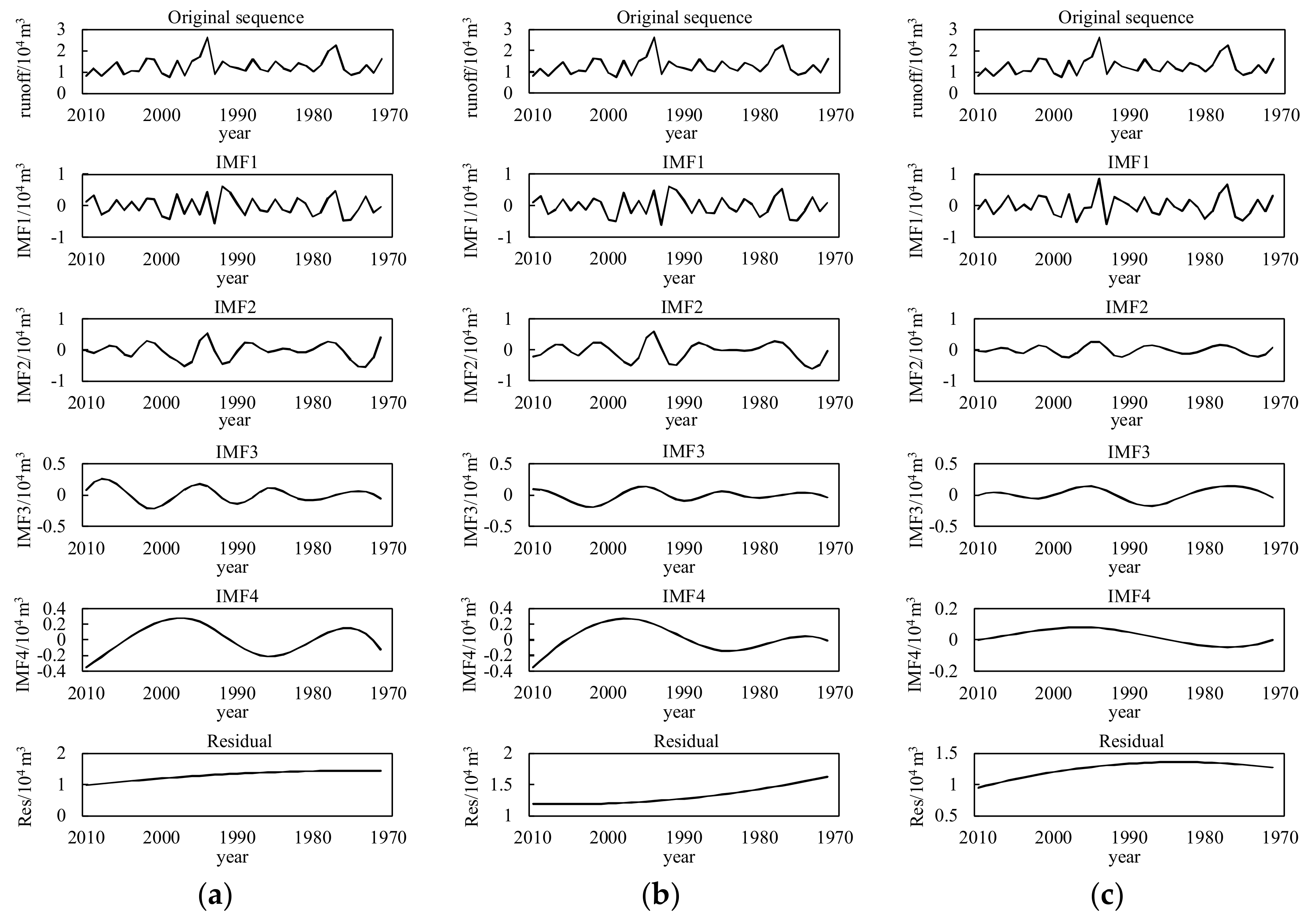
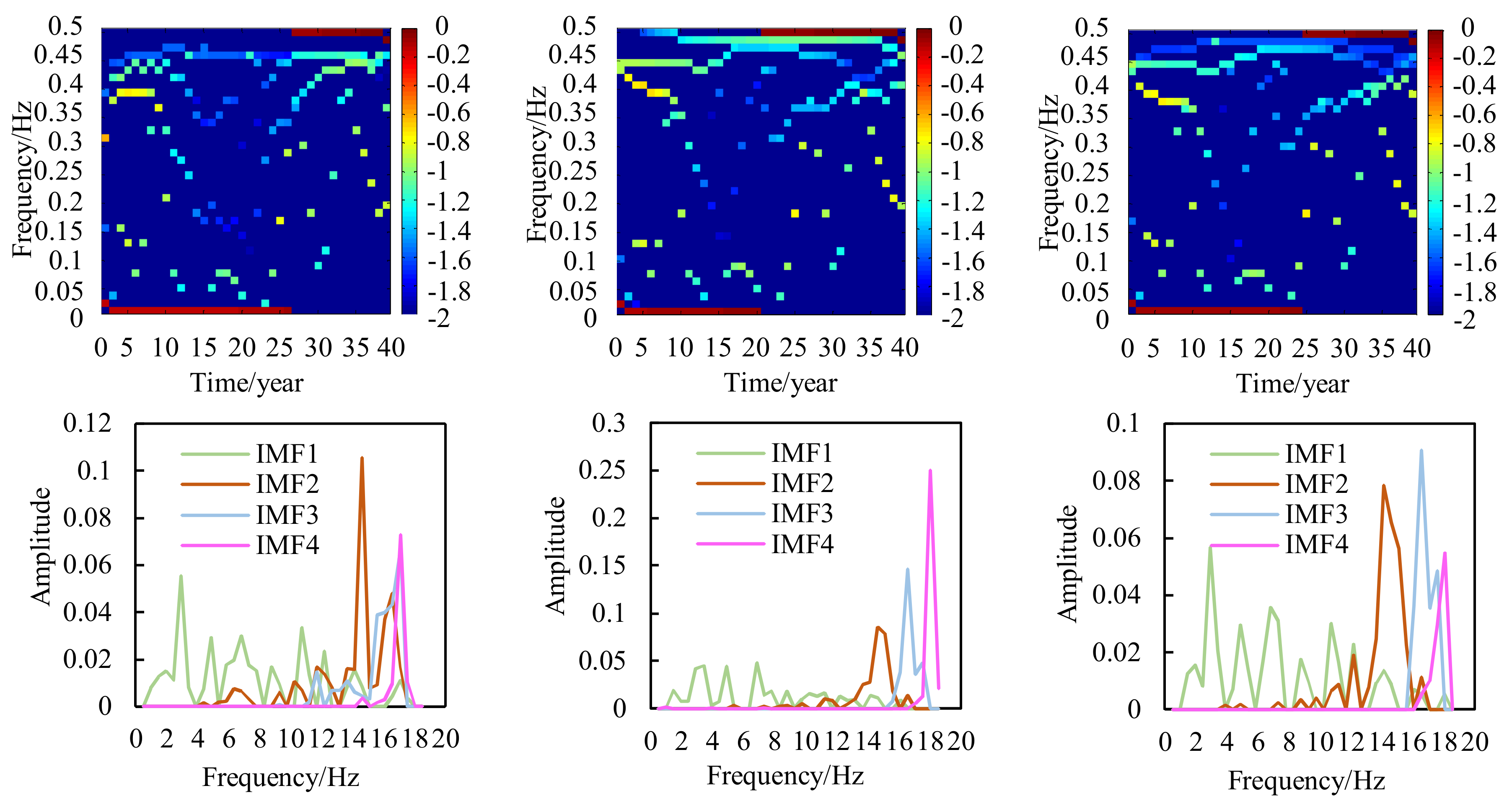
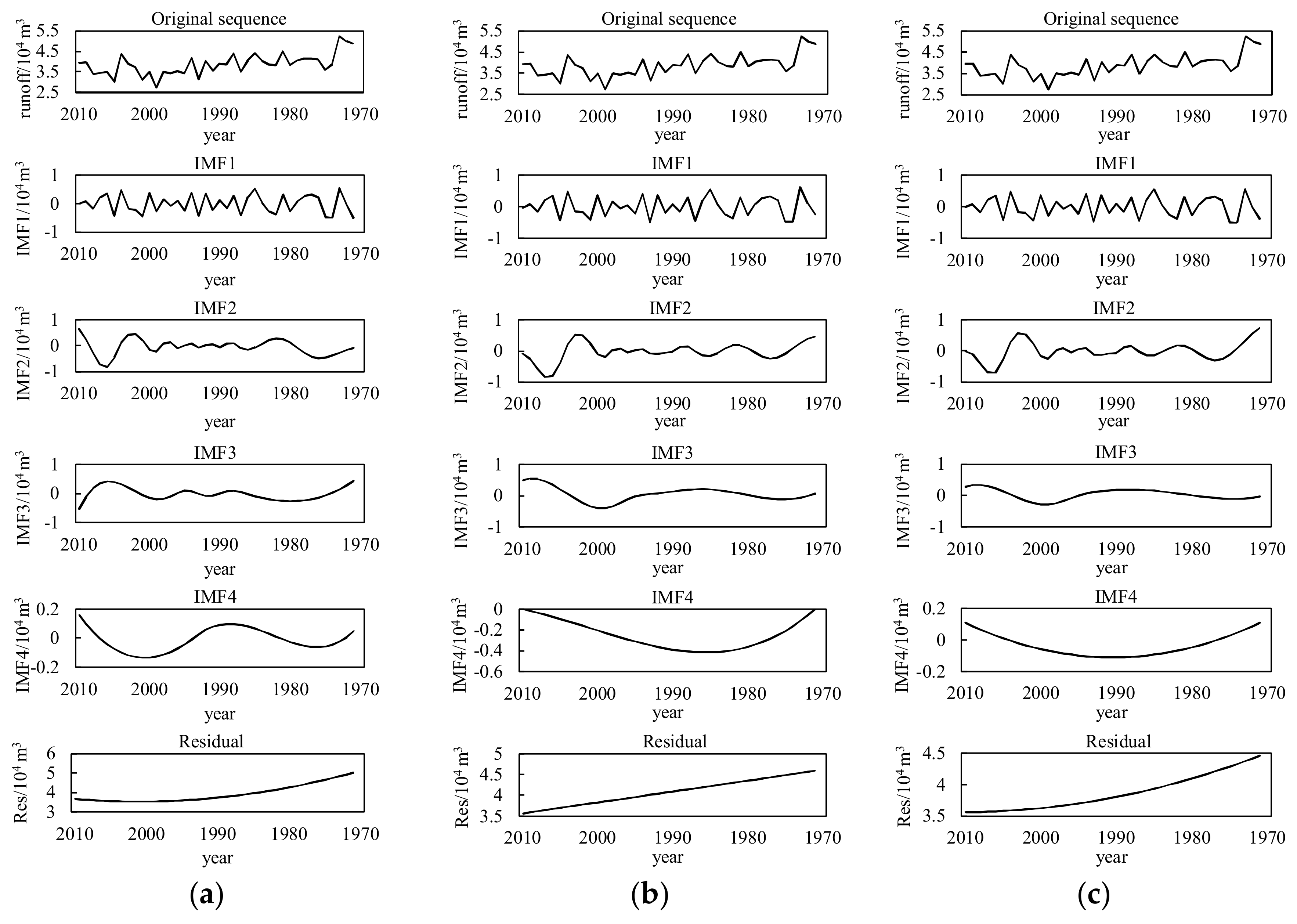
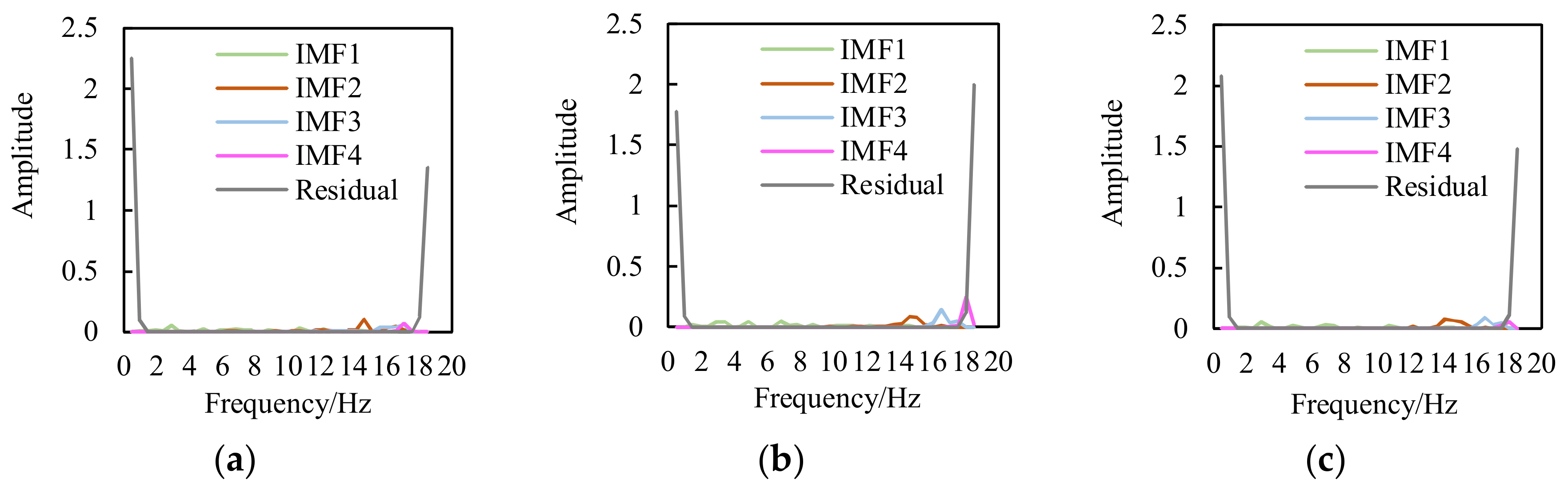
3.2.1. Improved EEMD

The annual runoff data in 1971–2010 at two hydrological stations were reversed and decomposed using the improved EEMD method. The MTED was used as the stopping criteria for EEMD sifting. To verify the decomposition performance by the improved EEMD method, the results were compared with the results obtained by decomposition methods based on the SD criteria and the GR criteria, as shown in Figure 1 and Figure 2.

In Figure 1a,b and Figure 2a,b show SD and GR criteria-based EEMD components, respectively, and Figure 1c and Figure 2c shows the MTED-based components. These figures show that with the three sifting stopping criteria, four IMFs and one residual can be obtained from decomposition. However, the same original series were decomposed into different components (different IMFs and different residuals) based on the three sifting stopping criteria. When the SD criteria or the GR criteria was used as the EEMD sifting stopping criteria, the decomposed components were highly fluctuating and irregular. In particular, in the low frequency component (such as IMF4), the decomposed components exhibited irregular waveforms. In other words, SD and GR criteria-based components exhibited severe mode mixing such that this did not accurately show hydrological fluctuations or periodical changes. Such fluctuating and irregular components were difficult to predict due to their weak regularity. In contrast, the components obtained by the MTED were relatively stable, fluctuating around 0, and had regular waveforms. After several rounds of sifting, the low-frequency components demonstrated regular sinusoidal fluctuations. This means that the EEMD results obtained by the MTED were better because mode mixing in the process was suppressed effectively, and the decomposed IMF component was more stable, which provided a solid foundation for forward prediction in the next stage. It is worth mentioning that the extraction of each component except IMF1 is based on the previous extracted component in the decomposition process of EMD. Different sifting stopping criteria could make extraction different, and the difference will enlarge along with the decomposition. Although the difference is not obvious among the high-frequency components (such as IMF1 and IMF2) obtained under three criteria, it is an objective reality and would lead to the curves of the low-frequency components being obviously different, as shown in Figure 1 and Figure 2. Compared with the MTED, the low-frequency component obtained through SD- and GR-criteria show irregular fluctuations, which indicates that the MTED-based EMD performs better than SD and GR criteria-based EMD in separating the multi-time scale information from the original series.

To further verify the above statement, the orthogonality index Ort was used to evaluate the superiority of the three sifting stopping criteria. Ort is an index that evaluates the orthogonality of the IMF components, and its value closer to zero means that the IMF components are more orthogonal [40]. The principle is illustrated as follows [41]:

Original runoff data undergo EEMD, and then n IMF components and one residual are obtained. The corresponding formula is as follows:

$$X(t)={\displaystyle {\sum }_{q=1}^n{c}_q(t)+r(t)}$$

(10)

where c_q(t) is the q-th IMF and r(t) is the residual which is defined as the last IMF component, i.e., r(t) is defined as c_n+1(t). Then, the original runoff data are represented as follows:

$$X(t)={\displaystyle {\sum }_{q=1}^{n+1}{c}_q(t)}$$

(11)

The runoff data X(t) in the form of a square are as follows:

$$X^2(t)={\displaystyle {\sum }_{q=1}^{n+1}{c}_q^2(t)+2{\displaystyle {\sum }_{q=1}^{n+1}{\displaystyle {\sum }_{p=1}^{n+1}{c}_q(t)}{c}_p(t)}}(q\ne p)$$

(12)

If all the IMF components are orthogonal, then the second term on the right side of the equal sign in above formula should be zero. Therefore, the definition of the orthogonality index Ort is as follows:

$$\mathrm{Ort}={\displaystyle {\sum }_{t=1}^N\left(\frac{{\displaystyle {\sum }_{p=1}^{n+1}{\displaystyle {\sum }_{q=1}^{n+1}{c}_p(t)}{c}_q(t)}}{X^2(t)}\right)}(p\ne q)$$

(13)

where N is the length of the runoff series.

Next, all IMFs and residuals decomposed with the three sifting stopping criteria are taken through the Hilbert–Huang transform (HHT) to obtain their Hilbert spectrum [26]. After integrating the Hilbert spectrum with respect to time, their Hilbert marginal spectrum is obtained, respectively, as shown in Figure 3 and Figure 4, in which it is seen that the Hilbert spectrum accurately reflects variations in the component’s amplitude with time and frequency. The marginal spectrum statistically represents the accumulated amplitude distribution of each component along the frequency. The orthogonality of the components is represented by the coincidence of major frequencies in the marginal spectrum. A smaller coincidence means the orthogonality is superior.

Table 1. Orthogonality index of runoff components based on three stopping criteria.

Orthogonality Index	Zhaoshiyao Station			Suide Station
	SD Criteria	GR Criteria	MTED	SD Criteria	GR Criteria	MTED
Without residual	−0.10	−0.10	−0.08	−1.24	−0.95	−0.23
With residual	−1.72	−3.57	−0.66	−8.63	−9.86	−5.64

lists the orthogonality indexes of the EEMD results with three sifting stopping criteria at the two hydrological stations. “With the residual” means the residual is used as the last IMF component in the calculation, and “without the residual” represents the fact that the residual has been removed, and other IMFs are used in the calculation. It can be found whether or not the residual is taken into the calculation, the MTED-based orthogonality index is closer to 0 than the indexes by the SD criteria and the GR criteria. This indicates that, compared with the SD criteria-based or GR criteria-based decomposition components, the MTED-based components are more orthogonal or with less mode mixing. This statement is also supported to a certain extent in Figure 3 and Figure 4. In the Hilbert spectrum of two figures, the horizontal axis represents time, the vertical axis represents frequency, and the depth of the color describes the magnitude of the amplitude. Although the Hilbert spectrums of three stopping criteria do not show a significant difference, it can be seen that the spectrum of the MTED-based components are more recognizable and regular than SD criteria-based and GR criteria-based components. Furthermore, a more significant superiority of MTED to SD criteria and GR criteria can be seen in the marginal spectrum, in which the dominant frequency and frequency band of each component can be recognized well. As shown in the marginal spectrum of Figure 3 and Figure 4, the dominant frequency of MTED-based components is significant while that of SD criteria-based and GR criteria-based components is difficult to distinguish. The detailed representation is as follows: the frequency band of MTED-based components is distributed relatively independently on different frequencies while that of SD criteria-based and GR criteria-based components overlap in the frequency range. In other words, Figure 3 and Figure 4 show that MTED-based decomposition is superior to SD criteria-based and GR criteria-based decomposition in decomposing the original series into several components corresponding to different frequency bands (different time scales). All these indicate that the SD criteria-based and GR criteria-based decomposition components have serious mode mixing and poor orthogonality. Fortunately, the MTED-based improved EEMD method can suppress mode mixing in the EEMD effectively, generating stable IMFs representing multi-scale physical information and thereby illustrating hydrological periodical change hidden in the runoff data to the extent possible.

3.2.2. Radial Basis Function (RBF) Neural Network and Autoregression (AR) Model Prediction

The data of runoff components (1981–2010) decomposed by the improved EEMD were used as training data. Through training, a RBF neural network and AR model was built and used for the prediction, in which the RBF neural network was employed to forward predict or extend the IMF1 data during non-observed period (1971–1980) by coupling the rainfall data in the same period, and the AR model was used to forward predict or extend other components’ data (IMF2–4 and the residual) during the non-observed period. Next, all the predicted runoff components were combined to obtain the predicted annual runoff data for the non-observed period.

To verify the prediction effect and compare the impact of three sifting stopping criteria (the SD criteria, the GR criteria and the MTED) on runoff prediction, the prediction results by the EEMD prediction models with three criteria were compared, as listed in

Table 2. Error assessment of improved EEMD prediction models based on three stopping criteria.

Error Evaluation Index	Zhaoshiyao Station			Suide Station
	SD Criteria	GR Criteria	MTED	SD Criteria	GR Criteria	MTED
Relative average deviation (RAD)/%	9.45	9.39	6.86	25.24	25.60	11.10
Nash–Sutcliffe efficiency (NSE)	0.19	−0.24	0.40	0.34	0.29	0.89

. Here, measured runoff data in the verification period were used as the benchmark for error analysis, and the relative average deviation (RAD) and the Nash–Sutcliffe efficiency (NSE) were used as error evaluation indexes to undertake comprehensive measurement and evaluation of the prediction performance. A smaller RAD and a larger NSE represent higher prediction precision.

Table 2 shows the prediction performance of EEMD prediction models based on the SD criteria, the GR criteria and the MTED, where it is clear that the MTED-based EEMD prediction model has significantly more precision than the SD-based and GR-based models. This also supports the inference about the applicability and superiority of MTED as a stopping criteria for EMD sifting.

3.3. Result Verification

To further verify the prediction performance of the improved EEMD prediction model, two common forward prediction methods used in engineering design (the rainfall-runoff method and the AR model) were selected for comparison, and measured runoff data during 1971–1980 were used for verification. The rainfall-runoff method is primarily based on the rainfall-runoff correlation in the research basin. Rainfall data was measured data in the study basin, and hence the missing annual runoff data can be predicted by the rainfall-runoff regression equation established in the training period (1981–2010). In the AR model, the measured runoff data from 1981 to 2010 were first sorted in reverse time order. After determining the three most significant orders as model inputs, the reverse data were implemented in the AR procedure to estimate the missing runoff data from 1980 to 1971.

Table 3. Error assessment of forward prediction by three models.

Error Evaluation Index	Zhaoshiyao Station			Suide Station
	AR Model Method	Rainfall-Runoff Method	Improved EEMD Prediction Model	AR Model Method	Rainfall-Runoff Method	Improved EEMD Prediction Model
RAD/%	11.03	15.13	6.86	27.76	19.67	11.10
NSE	−0.87	−1.54	0.40	−0.02	−0.11	0.89

lists the results of evaluation by error in the prediction by the three forward prediction methods. It shows that compared with the conventional rainfall-runoff method and the AR model method, the improved EEMD prediction model had more precise prediction.

To test the usefulness of these three forward prediction methods in engineering design, 40-year (1971–2010) runoff data series were generated, including 10-year predicted runoff data and 30-year measured data, and these were then compared with 40-year measured runoff data via statistical parameters. The results are shown in

Table 4. Statistical parameters between extended runoff series by different models and observed series at the Zhaoshiyao and Suide stations.

Statistical Parameters	Zhaoshiyao Station			Suide Station
	Mean	Mean Square Error	Coefficient of Variation	Mean	Mean Square Error	Coefficient of Variation
Original sequence	3.86	0.51	0.13	1.28	0.40	0.31
Improved EEMD prediction model	3.84	0.44	0.11	1.29	0.39	0.30
Rainfall-runoff method	3.70	0.38	0.10	1.22	0.33	0.27
AR model	3.75	0.37	0.10	1.26	0.33	0.26

.

The table shows that the extended long runoff series by the improved EEMD model had similar statistical parameters with the measured runoff data. If the designer used the extended data by the improved EEMD prediction model for engineering design, he would get a better hydrological design value to meet the engineering design requirements than by using the other two methods. However, the designer is likely to result in design deviation and put the project at risk if he adopted the extended data by the other two methods in order to undertake engineering design. Therefore, the improved EEMD model is undoubtedly a better choice for engineering design and hydrological research when hydrological data is scarce in a basin or region similar to north-west China, by which the obtained design value has a significant advantage for the regional water resource supply-demand balance and the safety of hydraulic project operation.

4. Conclusions

In this paper a new method, called the improved EEMD prediction model, is proposed to forward predict or extend runoff series in data-scarce basins for serving regional hydraulic engineering design. The model combines ensemble empirical mode decomposition (EEMD), a radial basis function (RBF) neural network, and an auto-regression (AR) model, whereby the EEMD is employed for decomposition and reconstruction, and the RBF and AR model are employed for forward predicting or extending the IMFs and residual components. Also, three EMD sifting stopping criteria (the SD criteria, the GR criteria and the MTED) are discussed and compared in this study to find the best criteria to solve the problem of mode mixing and improve the decomposition quality of EEMD. Additionally, two quantitative evaluation measures, the relative average deviation (RAD) and the Nash–Sutcliffe efficiency (NSE), are used to evaluate the performance of the improved prediction model and compare them with the AR model and a rainfall-runoff method.

The case study at two hydrological gauges located in north-west China, the Zhaoshiyao and Suide stations, indicates that: (1) the improved EEMD using the MTED as sifting stopping criteria suppresses mode mixing effectively (|Ort| < 0.23), ensuring that the IMFs are quasi-stable to preserve the physical information and periodical change contained in the runoff data to the extent possible; (2) the improved EEMD prediction model has lower RAD and NSE statistics, 6.86% and 0.40 at the Zhaoshiyao station, respectively, and 11.10% and 0.89 at the Suide station, respectively, and these are significantly better than the rainfall-runoff method and the AR model.

Comparative results indicate that this forward prediction model is undoubtedly a better choice for engineering design and hydrological research when hydrological data is scarce in a basin or region similar to north-west China.

References

- Sivapalan, M.; Takeuchi, K.; Franks, S.W.; Gupta, V.K.; Karambiri, H.; Lakshmi, V.; Liang, X.; Mcdonnell, J.J.; Mendiondo, E.M.; O’Connell, P.E. Iahs decade on predictions in ungauged basins (pub), 2003-2012: Shaping an exciting future for the hydrological sciences. Int. Assoc. Sci. Hydrol. Bull. 2003, 48, 857–880. [Google Scholar] [CrossRef]
- Montanari, A.; Young, G.; Savenije, H.H.G.; Hughes, D.; Wagener, T.; Ren, L.L.; Koutsoyiannis, D.; Cudennec, C.; Toth, E.; Grimaldi, S. “Panta rhei-everything flows”: Change in hydrology and society-the iahs scientific decade 2013-2022. Int. Assoc. Sci. Hydrol. Bull. 2013, 58, 1256–1275. [Google Scholar] [CrossRef]
- Servat, E.; Dezetter, A. Rainfall-runoff modelling and water resources assessment in northwestern ivory coast. Tentative extension to ungauged catchments. J. Hydrol. 1993, 148, 231–248. [Google Scholar] [CrossRef]
- Mcintyre, N.; Lee, H.; Wheater, H.; Young, A.; Wagener, T. Ensemble predictions of runoff in ungauged catchments. Water Resour. Res. 2005, 41, 4203–4206. [Google Scholar] [CrossRef]
- Wan, Y.; Konyha, K. A simple hydrologic model for rapid prediction of runoff from ungauged coastal catchments. J. Hydrol. 2015, 528, 571–583. [Google Scholar] [CrossRef]
- Li, F.; Zhang, Y.; Xu, Z.; Liu, C.; Zhou, Y.; Liu, W. Runoff predictions in ungauged catchments in southeast tibetan plateau. J. Hydrol. 2014, 511, 28–38. [Google Scholar] [CrossRef]
- Liu, C.; Bai, P.; Wang, Z.; Liu, S.; Liu, X. Study on prediction of ungaged basins: A case study on the tibetan plateau. J. Hydraul. Eng. 2016, 47, 272–282. [Google Scholar]
- Besaw, L.E.; Rizzo, D.M.; Bierman, P.R.; Hackett, W.R. Advances in ungauged streamflow prediction using artificial neural networks. J. Hydrol. 2010, 386, 27–37. [Google Scholar] [CrossRef]
- Mohamoud, Y. Prediction of daily flow duration curves and streamflow for ungauged catchments using regional flow duration curves. Int. Assoc. Sci. Hydrol. Bull. 2008, 53, 706–724. [Google Scholar] [CrossRef]
- Gazzaz, N.M.; Yusoff, M.K.; Aris, A.Z.; Juahir, H.; Ramli, M.F. Artificial neural network modeling of the water quality index for kinta river (malaysia) using water quality variables as predictors. Mar. Pollut. Bull. 2012, 64, 2409–2420. [Google Scholar] [CrossRef] [PubMed]
- Kalin, L.; Isik, S.; Schoonover, J.E.; Lockaby, B.G. Predicting water quality in unmonitored watersheds using artificial neural networks. J. Environ. Qual. 2010, 39, 1429–1440. [Google Scholar] [CrossRef] [PubMed]
- Noori, N.; Kalin, L. Coupling swat and ann models for enhanced daily streamflow prediction. J. Hydrol. 2016, 533, 141–151. [Google Scholar] [CrossRef]
- Palani, S.; Tkalich, P.; Balasubramanian, R.; Palanichamy, J. Ann application for prediction of atmospheric nitrogen deposition to aquatic ecosystems. Mar. Pollut. Bull. 2011, 62, 1198–1206. [Google Scholar] [CrossRef] [PubMed]
- Sahoo, G.B.; Ray, C.; Carlo, E.H.D. Use of neural network to predict flash flood and attendant water qualities of a mountainous stream on oahu, hawaii. J. Hydrol. 2006, 327, 525–538. [Google Scholar] [CrossRef]
- Asefa, T.; Kemblowski, M.; Mckee, M.; Khalil, A. Multi-time scale stream flow predictions: The support vector machines approach. J. Hydrol. 2006, 318, 7–16. [Google Scholar] [CrossRef]
- Jajarmizadeh, M.; Lafdani, E.K.; Harun, S.; Ahmadi, A. Application of svm and swat models for monthly streamflow prediction, a case study in south of iran. KSCE J. Civ. Eng. 2015, 19, 345–357. [Google Scholar] [CrossRef]
- Kalra, A.; Ahmad, S. Using oceanic-atmospheric oscillations for long lead time streamflow forecasting. Water Resour. Res. 2009, 45, 450–455. [Google Scholar] [CrossRef]
- Noori, R.; Karbassi, A.R.; Moghaddamnia, A.; Han, D.; Zokaei-Ashtiani, M.H.; Farokhnia, A.; Gousheh, M.G. Assessment of input variables determination on the svm model performance using pca, gamma test, and forward selection techniques for monthly stream flow prediction. J. Hydrol. 2011, 401, 177–189. [Google Scholar] [CrossRef]
- Manuca, R.; Savit, R. Stationarity and nonstationarity in time series analysis. Phys. D Nonlinear Phenom. 1996, 99, 134–161. [Google Scholar] [CrossRef]
- Trenberth, K.E. Recent observed interdecadal climate changes in the northern hemisphere. Bull. Am. Meteorol. Soc. 1990, 71, 377–390. [Google Scholar] [CrossRef]
- Tsonis, A.A. Widespread increases in low-frequency variability of precipitation over the past century. Nature 1996, 382, 700–702. [Google Scholar] [CrossRef]
- Kumar, P.; Foufoula-Georgiou, E. A multicomponent decomposition of spatial rainfall fields: 1. Segregation of large- and small-scale features using wavelet transforms. Water Resour. Res. 1993, 29, 2515–2532. [Google Scholar] [CrossRef]
- Saco, P.; Kumar, P. Coherent modes in multiscale variability of streamflow over the united states. Water Resour. Res. 2000, 36, 1049–1068. [Google Scholar] [CrossRef]
- Sang, Y.F.; Wang, Z.; Liu, C. Discrete wavelet-based trend identification in hydrologic time series. Hydrol. Process. 2013, 27, 2021–2031. [Google Scholar] [CrossRef]
- Wang, W.; Jing, D. Wavelet network model and its application to the prediction of hydrology. Nat. Sci. 2003, 1, 67–71. [Google Scholar]
- Huang, N.E.; Shen, Z.; Long, S.R.; Wu, M.C.; Shih, H.H.; Zheng, Q.; Yen, N.C.; Chi, C.T.; Liu, H.H. The empirical mode decomposition and the hilbert spectrum for nonlinear and non-stationary time series analysis. Proc. Math. Phys. Eng. Sci. 1998, 454, 903–995. [Google Scholar] [CrossRef]
- Sang, Y.F.; Wang, Z.; Liu, C. Comparison of the mk test and emd method for trend identification in hydrological time series. J. Hydrol. 2014, 510, 293–298. [Google Scholar] [CrossRef]
- Sang, Y.F.; Wang, Z.; Liu, C. Period identification in hydrologic time series using empirical mode decomposition and maximum entropy spectral analysis. J. Hydrol. 2012, s 424–425, 154–164. [Google Scholar] [CrossRef]
- Huang, Y.; Schmitt, F.G.; Lu, Z.; Liu, Y. Analysis of daily river flow fluctuations using empirical mode decomposition and arbitrary order hilbert spectral analysis. J. Hydrol. 2009, 373, 103–111. [Google Scholar] [CrossRef]
- Li, X.; Ding, Z. Emd method for multiple time-scale analysis on fluctuation characteristic of natural annual runoff time series of fen river. Water Resour. Power 2008, 30–32. [Google Scholar]
- Huang, S.; Chang, J.; Huang, Q.; Chen, Y. Monthly streamflow prediction using modified emd-based support vector machine. J. Hydrol. 2014, 511, 764–775. [Google Scholar] [CrossRef]
- Karthikeyan, L.; Kumar, D.N. Predictability of nonstationary time series using wavelet and emd based arma models. J. Hydrol. 2013, 502, 103–119. [Google Scholar] [CrossRef]
- Zhang, H.; Singh, V.P.; Wang, B.; Yu, Y. Ceref: A hybrid data-driven model for forecasting annual streamflow from a socio-hydrological system. J. Hydrol. 2016, 540, 246–256. [Google Scholar] [CrossRef]
- Huang, N.E. A study of the characteristics of white noise using the empirical mode decomposition method. Proc. Math. Phys. Eng. Sci. 2004, 460, 1597–1611. [Google Scholar]
- Wu, Z.; Huang, N.E. Ensemble empirical mode decomposition: A noise-assisted data analysis method. Adv. Adapt. Data Anal. 2005, 1, 1–41. [Google Scholar] [CrossRef]
- Huang, N.E.; Shen, Z.; Long, S.R. A new view of nonlinear water waves: The hilbert spectrum1. Ann. Rev. Fluid Mech. 1999, 31, 417–457. [Google Scholar] [CrossRef]
- Gabriel, R.; Patrick, F.; Paulo, G. On empirical mode decomposition and its algorithms. In Proceedings of the IEEE-EURASIP Workshop on Nonlinear Signal and Image Processing (NSIP-03), Grado, Italy, 8–11 June 2003. [Google Scholar]
- Cheng, J. Research on Fault Diagnosis Methods for Rotating Machinery Based on Hilbert-Huang Transform; Hunan University: Changsha, China, 2005. [Google Scholar]
- Pan, W. Akaike’s information criteria in generalized estimating equations. Biometrics 2001, 57, 120–125. [Google Scholar] [CrossRef] [PubMed]
- Ahmed, N.; Rao, K.R.; Debnath, L. Orthogonal transforms for digital signal processing. IEEE Trans. Syst. Man Cybern. 1976, 9, 66–67. [Google Scholar] [CrossRef]
- Li, X. Study on Orthogonality of Emd Method in Hht; Kunming University Of Science And Technology: Kunming, China, 2010. [Google Scholar]