Modeling Soil Water Dynamics and Pasture Growth in the Montado Ecosystem Using MOHID Land

Abstract

The southern Iberian Peninsula is characterized by evergreen oak woodlands (locally known as montado), which constitute an important savanna-type agro-silvo-pastoral ecosystem. This ecosystem is facing a progressive decline for several reasons, with the foremost being overgrazing. Better management tools are necessary to accurately quantify the systems’ carrying capacity and the sustainable stocking rates that prevent land degradation. The purpose of this study was to determine whether the MOHID-Land model could adequately simulate soil water dynamics and pasture growth in the montado ecosystem. The study area was located in the Alentejo region of southern Portugal. The model successfully simulated soil water contents and aboveground biomass during the 2010–2011 and 2011–2012 growing seasons, producing acceptable errors of the estimates (0.015 ≤ RMSE ≤ 0.026 cm³ cm⁻³; 279 ≤ RMSE ≤ 1286.5 kg ha⁻¹), and relatively high modeling efficiencies (0.481 ≤ EF ≤ 0.882). The model was further used to simulate the same variables for a longer period (1979/2009 seasons), to account for the effect of climate variability on model estimates. Water balance and dry biomass estimates were found to be significantly different between rainfed and irrigated pastures, as well as between the ten driest and ten wettest seasons, with the model responding well to climate variability. The results showed the potential of using the MOHID-Land model for improving pasture management in the montado ecosystem.

1. Introduction

The southern region of the Iberian Peninsula is characterized by a savanna-type agro-silvo-pastoral ecosystem, known as montado in Portugal (hereafter adopted) and dehesa in Spain [1,2]. The montado system consists of an open formation of cork (Quercus suber L.) and holm oak (Quercus ilex rotundifolia L.) trees, presenting high levels of spatial variability in terms of density, combined with fallow land or pastures, which can be natural, improved, or cultivated [3,4]. The structural diversity of the system combines with the good overall habitat connectivity over its area of distribution, allowing animals to move around their territories, find mates, hunt, forage, and reproduce, resulting in high levels of biodiversity. As a result, the montado is considered as a High Natural Value system [2], providing various ecosystem services (ES) that are perceived by farmers, stakeholders, and society in general as being important for human welfare [5,6,7].

In the last decades, the implementation of the European Common Agricultural Policy has led to an intensification of grazing, which has caused additional stress to the system, promoting the spread of tree diseases and preventing the natural regeneration of the ecosystem [3,4,8]. The most significant transformations have been (i) the increase of the stocking (or livestock) pressure (i.e., the replacement of sheep by cattle, the replacement of light indigenous breeds of cattle by heavier breeds, and the increase of livestock units per area); and (ii) the use of heavy machinery for shrub control [7]. These changes have exhausted the natural pastures, decreased tree regeneration, and degraded water and soil quality [3,7]. Therefore, there is the need for the development of policy instruments that consider the specificities of the montado silvopastoral system; otherwise, its future will be severely threatened in the short term [5,7,9].

One major challenge for improving system management is understanding soil water dynamics in the pasture component of the montado ecosystem, allowing for its improved management regarding grazing, and hence its capacity to withstand increased stocking pressure. Mediterranean grassland species have evolved adaptive strategies to avoid or endure severe summer droughts, adjusting their lifecycle to seasonal water availability [10]. The emergence of plants depends on the timing of the first autumn precipitations, and their active period is in winter and early spring, with senescence in May [11,12,13,14]. In montado systems, the understory plays an important role in the functioning of the ecosystem [12], having a variable productivity that responds to the temperature and precipitation (P) regimes. The relationship between soil water and biomass also influences whether these ecosystems act as CO₂ source or sink, with Jongen et al. [12] suggesting that in dry years grasslands may act as a source of CO₂, while in more humid years they may act as a sink. With climate change scenarios suggesting a decrease in annual precipitation in mid-latitude temperate regions, accompanied by increasing temporal variability of precipitation and drought risks [14,15,16], it is thus essential to develop tools for accurately quantifying the soil water balance and net primary production, and improving system management. The additional variability in precipitation also introduces the possibility of an additional management alternative: the use of of irrigated pastures. These both allow a smoothing of the effects of precipitation variability in rainfed pastures and provide a buffer of forage production, to release grazing pressure from rainfed pastures when that production is inadequately high.

Today, several process-based models, such as the BIOME–BGC [17], STICS [18], SPACSYS [19], EPIC [20], ARMOSA [21], and PaSim [22] models, are available for simulating soil water dynamics and vegetation growth in grasslands. Most of these models provide an integrated perspective by taking into account the various vegetation, soil, and weather processes regulating energy and matter exchanges in agroecosystems. Some of these processes though, as in the cases of the EPIC [20] and PaSim [22] models, are described in a simplistic way. For example, soil water dynamics is usually defined based on the notion of field capacity and the wilting point, with soil water storage capacity being computed from atmospheric demands, while other outputs, such as capillary rise and percolation, are computed empirically. Other process-based models, such as SPACSYS [19], and ARMOSA [21], make use of the Richards equation for computing soil water dynamics, thereby providing a more physically-based approach for predicting soil water contents and fluxes. Another example is the MOHID-Land model [23], which is a distributed model based on primitive equations for surface runoff and flow in both the vadose zone and the aquifer. Flow in porous media is based on the Richards equation, while infiltration can be simulated using Darcy’s equation and surface pressure, due to the surface runoff water column or by using empirical algorithms (e.g., Green and Ampt). The MOHID-Land model further includes a modified version of the EPIC model [20] for simulating crop development and biomass growth, which can potentially be used for estimating the stocking rates in the montado ecosystem and prevent soil degradation.

Hence, the objectives of this study were (i) to calibrate/validate the process-based MOHID-Land model [23] for estimating soil water dynamics and dry biomass growth in a rainfed and irrigated pasture during the 2010–2011 and 2011–2012 seasons; (ii) to estimate pasture irrigation (I) needs, using the calibrated model for the 1979–2009 seasons (30 years); and (iii) to compare the soil water balance and dry biomass estimates in rainfed and irrigated pastures during both wet and dry seasons, providing an insight on the influence of climate variability on model performance. The hypotheses addressed in this study were (i) that the MOHID-Land model could accurately estimate the soil water balance and aboveground biomass growth in pastures under different management regimes; (ii) that the model could be used for irrigation scheduling; and (iii) that climate variability had a significant effect on model estimates. The results of this study will help to support the decision-making process regarding ecosystem management, by better accounting for the stocking rates and reducing the adverse impact of grazing in the montado ecosystem.

2. Material and Methods

2.1. Field Site Description and Data

The field data was collected at Herdade da Machoqueira do Grou, located near Coruche, southern Portugal (39°08′16″ N, 08°20′03″ W). The climate in the region is dry and sub-humid, with mild winters and hot, dry summers. The mean annual temperature is 15.9 °C, with the mean daily temperatures at the coolest (December) and warmest (August) months being 10.4 and 23.8 °C, respectively. The mean annual precipitation is 680 ± 210 mm, with 87% falling between October and May (over the 1955–2007 period). The weather variables (rainfall (mm), average temperature (°C), wind speed (m s⁻¹), relative humidity (%), and solar radiation (W m⁻²)) were provided for the study area by the MM5 mesoscale model (http://meteo.tecnico.ulisboa.pt), forced by the initial conditions from the NCEP (National Centers for Environmental Predition) Climate Forecast System Reanalysis, at a spatial resolution of 9 km.

The soil was classified as a Cambisol [24]. The main physical and chemical properties of the soil are presented in

Table 1. Main physical and chemical soil characteristics.

Soil Properties	Soil Layers
Depth (m)	0–0.2	0.2–0.8	>0.8
Coarse sand, 2000–200 μm (%)	65.83	56.18	63.43
Fine sand, 200–20 μm (%)	21.70	21.64	13.91
Silt, 20–2 μm (%)	10.98	17.34	9.35
Clay, <2 μm (%)	1.49	9.35	13.30
Texture	Loamy-sand	Sandy-loam	Sandy-loam
Bulk density (g cm−3)	1.65	1.57	-
Organic matter (%)	1.39	0.32	0.02

. The particle size distribution was determined using the pipette method [25] for particles with a diameter of <2 μm (clay fraction) and between 20 and 2 μm (silt), and by sieving for particles between 200 and 20 μm (fine sand) and between 2000 and 200 μm (coarse sand). These textural classes follow the Portuguese classification system [26], and are based on international soil particle limits (Atterberg scale). The dry bulk density (ρ_g, cm⁻³) was obtained by the core method [25] (soil samples of 100 cm³). The organic matter (OM, %) content was estimated from the organic carbon (OC, %) content determined by the Walkley–Black method, using the relation OM = 1.724 × OC [27].

Montado, with a density of Quercus suber (170 trees/ha), was the main land use at the field site. The understory vegetation and grassland was a mixture of C3 annual species, which emerged after the first rains in autumn and senesced in late spring. Initially, the dominant species were Agrostis pourretii Willd., Plantago coronopus L., Rumex acetosella L., Tolpis barbata (L.) Gaertn., Tuberaria guttata (L.) Fourr., Vulpia bromoides (L.) S.F. Gray, and Vulpia geniculata (L.) Link. In October 2009, the site was ploughed and seeded with a biodiverse mixture of legumes (Biserrula pelecinum L., Ornithopus compressus L., Ornithopus sativus Brot., Trifolium subterraneum L., Trifolium michelanium—balansae (Boiss.) Azn., Trifolium incarnatum L., Trifolium glanduliferum Boiss., Trifolium resupinatum L., and Trifolium vesiculosum Savi.), with one grass species (Lolium multiflorum L.) [13]. By the 2010–2012 seasons, the dominant species were Agrostis pourretii Willd., Bartsia trixago L., Ornithopus pinnatus (Mill.) Druce, Ornithopus sativus Brot., Rumex acetosella L., Spergula arvensis L., Tolpis barbata (L.) Gaertn., and Tuberaria guttata (L.) Fourr. The vegetation was therefore mostly dominated by non-sown species.

The MOHID-Land model was calibrated/validated using data from Jongen et al. [13,14]. These authors carried out a rainfall manipulation experiment to study the resilience of montado understory to precipitation variability between October 2010 and June 2012. Eight rainfall manipulation shelters were constructed, each one covering an area of 6 m × 5 m (30 m²), within a fenced area of about 3500 m². The shelters were covered with a clear, 0.2 mm, UV-transparent polyethylene greenhouse film. More details related to the shelter design can be found in [13].

During the 2010–2011 and 2011–2012 growing seasons, the pasture within four manipulation shelters was irrigated every three weeks, receiving 40 mm per event, with this quantity being defined based on historical precipitation data (1955–2007). Hereafter, these plots will be referred to as “irrigated pasture”. Water was applied to the experimental plots using an irrigation system, consisting of four 18-VAN rotary sprinklers with 90° arc nozzles (Rainbird, Azusa, CA, USA), one in each corner of the experimental plots [14]. In addition, four non-sheltered “control” plots receiving natural precipitation were defined, referred to hereafater as rainfed pasture. All plots received an equal water input during the germination and seedling establishment (until the middle of November).

The soil volumetric water content was continuously measured (every 10 min) in the middle of each experimental plot with an EC-5 soil moisture sensor (Decagon Devices, Pullman, WA, USA). In the irrigated and rainfed plots, measurements were taken at 10 and 5 cm depth, respectively. Aboveground (ABG) dry biomass was measured four times per season. Two 30 cm × 30 cm quadrats were defined in each experimental plot. All plants inside were harvested, oven-dried at 60 °C for 72 h, and weighed. The maximum leaf area index (LAI_max, m² m⁻²) was measured using a ceptometer (AccuPAR model LP-80, Decagon Devices, Pullman, USA), allowing an indirect determination of LAI by measuring the fraction of intercepted, photosynthetically-active radiation of the canopy. Maximum root depth was estimated at the end of the growing season (12 June). In each of the experimental plots, three soil cores of 8 cm diameter and a depth of up to 20 cm were taken. Roots were washed out, with subsequent analysis of root length for determination of specific root length (SRL) using WinRhizo software (Regents Instruments Inc., Québec, QC, Canada), then oven dried at 60 °C for 72 h, and weighed [14].

2.2. Model Description

2.2.1. Soil Water Dynamics

MOHID-Land is an open-source, physically based, distributed model, which uses a finite-volume approach based on mass and momentum balance equations [23]. The variable-saturated one-dimensional water flow is described using the Richards equation:

$$\frac{\partial \theta }{\partial t}=\frac{\partial }{\partial \mathrm{z}}\left[\mathrm{K}\left(\mathrm{h}\right)\frac{\partial \mathrm{h}}{\partial \mathrm{z}}-\mathrm{K}\left(\mathrm{h}\right)\right]-\mathrm{S}\left(\mathrm{z},\mathrm{t}\right)$$

(1)

where θ is the volumetric soil water content (L³ L⁻³), t is time (T), z is the vertical space coordinate (L), h is the soil water pressure head (L), K is the hydraulic conductivity (L T⁻¹), and S is the sink term accounting for water uptake by plant roots (L³ L⁻³ T⁻¹). The unsaturated soil hydraulic properties are described using the van Genuchten–Mualem functional relationships [28]:

$${\mathrm{S}}_{\mathrm{e}}(\mathrm{h})=\frac{\theta (\mathrm{h})-{\theta }_{\mathrm{r}}}{{\theta }_{\mathrm{s}}-{\theta }_{\mathrm{r}}}=\frac{1}{{\left(1+\left|\alpha \mathrm{h}\right|{}^{\eta }\right)}^{\mathrm{m}}}$$

(2)

$$\mathrm{K}\left(\mathrm{h}\right)={\mathrm{K}}_{\mathrm{s}}{\mathrm{S}}_{\mathrm{e}}^{\ell }{\left[1-{\left(1-{\mathrm{S}}_{\mathrm{e}}^{1/\mathrm{m}}\right)}^{\mathrm{m}}\right]}^2$$

(3)

where S_e is the effective saturation (L³ L⁻³), θ_r and θ_s denote the residual and saturated water contents (L³ L⁻³), respectively, K_s is the saturated hydraulic conductivity (L T⁻¹), α (L⁻¹) and η (-) are empirical shape parameters, m = 1 − 1/η, and ℓ is a pore connectivity/tortuosity parameter (-).

The sink term (S) accounting for root water uptake in Equation (1) is computed using the macroscopic approach introduced by Feddes et al. [29]. In this approach, potential transpiration (T_p) is linearly distributed over the root zone, creating the function T_p(z), and may be diminished by the presence of depth-varying root zone stressors, namely water stress [29,30,31]. For that, crop evapotranspiration rates (ET_c, L T⁻¹) are computed with the FAO Penman–Monteith method, using the single crop coefficient approach [32], and partitioned into potential soil evaporation (E_p, L T⁻¹) and potential crop transpiration (T_p, L T⁻¹) as a function of LAI [33]:

$${\mathrm{T}}_{\mathrm{p}}={\mathrm{ET}}_{\mathrm{c}}\left(1-{\mathrm{e}}^{\left(-\lambda \mathrm{LAI}\right)}\right)$$

(4)

$${\mathrm{E}}_{\mathrm{p}}={\mathrm{ET}}_{\mathrm{c}}-{\mathrm{T}}_{\mathrm{p}}$$

(5)

where λ is the extinction coefficient of radiation attenuation within the canopy (-). Then, the actual transpiration rate (T_a, L T⁻¹) is obtained by integrating T_p(z) over the root domain, and by limiting it using the piecewise linear model proposed by Feddes et al. [29]. This approach considers that the water uptake is at the potential rate when the pressure head is between h₂ and h₃, drops off linearly when h > h₂ or h < h₃, and becomes zero when h < h₄ or h > h₁ (subscripts 1 to 4 denote for different threshold pressure heads). E_p is limited by a pressure head threshold value, in order to obtain the actual soil evaporation rate (E_a, L T⁻¹) [34].

2.2.2. Plant Growth

The MOHID-Land model includes a modified version of the EPIC model [20,35] for simulating crop growth. This model is based on the heat unit theory, which considers that all heat above the base temperature will accelerate crop growth and development:

$$\begin{array}{ll}\mathrm{PHU}={\displaystyle \sum _{\mathrm{i}=1}^{\mathrm{mat}}\mathrm{HU}}={\displaystyle \sum _{\mathrm{i}=1}^{\mathrm{mat}}}\left({\mathrm{T}}_{\mathrm{av}}{-\mathrm{T}}_{\mathrm{base}}\right)& \mathrm{when}{\mathrm{T}}_{\mathrm{av}}{\text{>}}_{\mathrm{base}}\\ \mathrm{PHU}=0& \mathrm{when}{\mathrm{T}}_{\mathrm{av}}\le {\mathrm{T}}_{\mathrm{base}}\end{array}$$

(6)

where PHU is the total heat units required for plant maturity (°C), HU is the number of heat units accumulated on day i (°C), i = 1 corresponds to the emergence date (-), mat is the number of days required for plant maturity (-), T_av is the mean daily temperature (°C), and T_base is the minimum temperature for plant growth (°C). Plant growth stages (initial, plant development, mid-season, and late season stages) are thus defined as a fraction of PHU.

Crop growth is modeled by simulated light interception, the conversion of intercepted light into biomass, and LAI development [35,36]. The change in total biomass is calculated from the solar radiation intercepted by the crop leaf area, using Beer’s law [37]:

$${\displaystyle \sum _{\mathrm{i}=1}^{\mathrm{mat}}{\mathsf{\Delta }\mathrm{BM}}_{\mathrm{act},\mathrm{i}}}={\displaystyle \sum _{\mathrm{i}=1}^{\mathrm{mat}}{\mathsf{\Delta }\mathrm{BM}}_{\mathrm{i}}}{\mathsf{\gamma }}_{\mathrm{i}}={\displaystyle \sum _{\mathrm{i}=1}^{\mathrm{mat}}\mathrm{RUE}\left(0.5{\mathrm{PAR}}_{\mathrm{day},\mathrm{i}}\left(1-{\mathrm{e}}^{\left(-\mathsf{\lambda }\mathrm{LAI}\right)}\right)\right){\mathsf{\gamma }}_{\mathrm{i}}}$$

(7)

where ΔBM_act,i and ΔBM_i are the actual and potential increase in total plant biomass on day i (kg ha⁻¹), RUE is the radiation-use efficiency of the plant ((kg ha⁻¹) (MJ m⁻²)⁻¹), PAR_day,i is the daily incident of photosynthetically-active radiation (MJ m⁻²), λ is again the light extinction coefficient (-), and γ_i is the daily plant growth factor (0–1), which accounts for water and temperature stresses. RUE is estimated using the approach proposed by Stockle et al. [38], while γ_i is computed as Neitsch et al. [35]:

$${\mathsf{\gamma }}_{\mathrm{i}}=1-\max \left({\mathrm{w}}_{\mathrm{strs},\mathrm{i}}{,\mathrm{t}}_{\mathrm{strs},\mathrm{i}}\right)$$

(8)

where w_strs,i and t_strs,i are the water and temperature stresses for a given day i (-), respectively. Water stress (w_strs,i) is calculated as in Neitsch et al. [35]:

$${\mathrm{w}}_{\mathrm{strs},\mathrm{i}}=1-\frac{{\mathrm{T}}_{\mathrm{a}\mathrm{cum},\mathrm{i}-1}}{{\mathrm{T}}_{\mathrm{p}\mathrm{cum},\mathrm{i}-1}}$$

(9)

where T_{a cum} and T_{p cum} are the cumulative T_a and T_p values on day i − 1 (note that, by construction, T_a < T_p, so water stress is bounded between 0 and 1). The effect of water stress on crop growth is thus only reflected on the following day. Temperature stress is computed as temperature divergence from the optimal (T_opt, °C) using a sigmoidal function, influencing crop development similarly to water stress [35]:

$$\begin{array}{ll}{\mathrm{t}}_{\mathrm{strs},\mathrm{i}}=1& \mathrm{when}{\mathrm{T}}_{\mathrm{av}}\le {\mathrm{T}}_{\mathrm{base}}\\ {\mathrm{t}}_{\mathrm{strs},\mathrm{i}}=1-\exp \left[\frac{-0.1054{\left({\mathrm{T}}_{\mathrm{opt}}-{\mathrm{T}}_{\mathrm{av}}\right)}^2}{{\left({\mathrm{T}}_{\mathrm{av}}-{\mathrm{T}}_{\mathrm{base}}\right)}^2}\right]& \mathrm{when}{\mathrm{T}}_{\mathrm{base}}\le {\mathrm{T}}_{\mathrm{av}}\le {\mathrm{T}}_{\mathrm{opt}}\\ {\mathrm{t}}_{\mathrm{strs},\mathrm{i}}=1-\exp \left[\frac{-0.1054{\left({\mathrm{T}}_{\mathrm{opt}}-{\mathrm{T}}_{\mathrm{av}}\right)}^2}{{\left(2{\mathrm{T}}_{\mathrm{opt}}-{\mathrm{T}}_{\mathrm{av}}-{\mathrm{T}}_{\mathrm{base}}\right)}^2}\right]& \mathrm{when}{\mathrm{T}}_{\mathrm{opt}}<{\mathrm{T}}_{\mathrm{av}}\le 2{\mathrm{T}}_{\mathrm{opt}}-{\mathrm{T}}_{\mathrm{base}}\\ {\mathrm{t}}_{\mathrm{strs},\mathrm{i}}=1& \mathrm{when}{\mathrm{T}}_{\mathrm{av}}>2{\mathrm{T}}_{\mathrm{opt}}-{\mathrm{T}}_{\mathrm{base}}\end{array}$$

(10)

where T_av is the mean air temperature for a given day (°C), and T_base is the plant’s minimum temperature for growth (°C), respectively.

Leaf area index is computed as a function of heat units and plant stress [35]. During early stages (initial and plant development stages), LAI increment on a given day is a function of the fraction of the plant’s maximum LAI (LAI_max, m² m⁻²) that needs to be reached during those stages (fr_LAImax,ini), as well as crop stress. During the mid-season stage, LAI is assumed to be constant, while during the late-season stage LAI declines as a function of LAI_max, PHU, and crop stress. Root depth is also computed as a function of heat units [35], while root biomass is assumed to decrease from 0.4 of the total biomass at emergence to 0.2 at maturity [39]. A more detailed description of MOHID-Land’s crop module governing equations can be found in Ramos et al. [36].

2.3. Model Setup, Calibration, and Validation

In the MOHID-Land model, the simulation period covered the 2010–2011 and 2011–2012 growing seasons, being set from emergence to senescence each year. The soil profile was specified with 4 m depth and divided into three soil layers (Table 1). The soil domain was represented using an Arakawa C grid type [40], defined by one vertical column discretized into 11 grid cells, 1 m wide, 1 m long, and with variable thickness (0.05 m on the top to 2.5 m at the bottom).

The upper boundary condition was determined by the actual evaporation and transpiration rates, as well as the irrigation and precipitation fluxes. ET_c values were computed by multiplying the daily reference evapotranspiration (ET₀) values with crop coefficients (K_c) for the initial (0.3), mid-season (0.7), and late season (0.7) stages. These values were taken from Allen et al. [32], and correspond to standard K_c values for pasture in the Mediterranean region. The K_c value for the initial stage was then adjusted for the frequency of the rainfall events and average infiltration depths, while the K_c values for mid-season and late season were adjusted for local climate conditionsm taking into consideration plant height, wind speed, and minimum relative humidity averages for the period under consideration [32]. Root water uptake reductions were computed by considering the following parameters: h₁ = −10, h₂ = −25, h₃ = −200 to −800, h₄ = −8000 cm [41].

Model calibration and validation were carried out during the 2010–2011 and 2011–2012 seasons, respectively, with procedures following Ramos et al. [36]. The soil hydraulic (

Table 2. Van Genuchten–Mualem parameters in irrigated and rainfed plots.

Parameter	Soil Layers
Depth (m)	0–0.2	0.2–0.8	>0.8
Irrigated Plots:
θr (cm3 cm−3)	0.035	0.035	0.067
θs (cm3 cm−3)	0.300	0.300	0.450
α (cm−1)	0.015	0.015	0.020
η (-)	1.80	1.80	1.41
ℓ (-)	0.50	0.50	0.50
Ks (cm d−1)	62.4	27.8	4.5
Rainfed Plots:
θr (cm3 cm−3)	0.035	0.035	0.067
θs (cm3 cm−3)	0.290	0.300	0.450
α (cm−1)	0.015	0.015	0.020
η (-)	1.85	1.80	1.41
ℓ (-)	0.50	0.50	0.50
Ks (cm d−1)	62.4	27.8	4.5

θ_r, residual water content; θ_s, saturated water content; α and η, empirical shape parameters; ℓ, pore connectivity/tortuosity parameter; K_s, saturated hydraulic conductivity.

) and the crop parameters (

Table 3. Optimized parameters of the crop growth model.

Crop Parameter	Irrigated Plot	Rainfed Plot
Optimal temperature for plant growth, Topt (°C)	20.0	20.0
Minimum temperature for plant growth, Tbase (°C)	5.0	5.0
Plant radiation-use efficiency, RUE [(kg ha−1) (MJ m−2)−1]	8.0	8.0
Total heat units required for plant maturity, PHU (°C)	1800	1800
Fraction of PHU to reach the end of stage 1 (initial crop stage), frPHU,init (-)	0.05	0.05
Fraction of PHU to reach the end of stage 2 (canopy development stage), frPHU,dev (-)	0.20	0.60
Fraction of PHU after which LAI starts to decline, frPHU,sen (-)	0.70	0.70
Maximum leaf area index, LAImax (m2 m−2)	3.0	3.0
Fraction of LAImax at the end of stage 1 (initial crop stage), frLAImax,ini (-)	0.05	0.05
Fraction of LAImax at the end of stage 2 (canopy development stage), frLAImax,dev (-)	0.55	0.40
Maximum canopy height, hc,max (m)	0.30	0.30
Maximum root depth, Zroot,max (m)	0.40	0.40

) were calibrated for both rainfed and irrigated plots (during the 2010–2011 growing season). A trial-and-error procedure was adopted. First, the parameters of the van Genuchten–Mualem equations (Equations (2) and (3)) were defined according to the average values proposed by Carsel and Parish [42] for each soil texture class. The soil hydraulic parameters θ_s, α, η, and K_s were then modified to reduce the deviation between the observed and the simulated soil water contents. The parameter θ_r was not modified, as it did not significantly influence soil moisture simulations. The ℓ parameter was set to 0.5, as suggested by Mualem [43]. The crop parameters were calibrated by optimizing the default values of the EPIC model for pasture [35] until the deviation between the simulated and the observed ABG dry biomass was minimized. The values of the LAI_max and maximum root depth were taken directly from Jongen et al. [13]. The calibrated model parameters were then validated during the 2011–2012 growing season and the statistical indicators (given below) computed.

The goodness-of-fit indicators adopted for comparing MOHID-Land model simulations with the observed values of θ and ABG dry biomass were the mean error (ME), the root mean square error (RMSE), the normalized RMSE (NRMSE), and the model efficiency (EF). ME values close to zero indicate no bias. RMSE and NRMSE values close to zero indicate small estimation errors and good model predictions [44,45,46]. EF values close to one indicate that the residuals’ variance is much smaller than the observed data variance, hence the model predictions are good. On the contrary, when EF is very close to 0 or negative, there is no gain in using the model [47].

2.4. Simulation Scenarios

After model calibration/validation, the MOHID-Land model was used to compute the water balance and dry biomass yields in rainfed and irrigated pastures, hypothetically grown in the studied area during the 1979–2009 seasons (30 years). Climatic data was also provided by the same numerical mesoscale MM5 used earlier (http://meteo.tecnico.ulisboa.pt), and expresses the typical climatic variability found in the Mediterranean region (Figure 1), with annual precipitation amounting to between 68 and 805 mm.

In irrigated pastures, irrigation needs were further computed with a system-dependent boundary condition that automatically triggered irrigation when a certain threshold pressure head (h_t) was obtained in different grid cells of the root zone domain. Irrigation then ceased after a second target pressure head (h₀) was obtained in the same grid cells. This system-dependent boundary condition further included a series of constraints that prevented the application of meaningless irrigation amounts and countless irrigation events, namely a minimum irrigation pulse (I_min), a maximum irrigation pulse (I_max), and a minimum irrigation interval (I_int). The model was thus capable of automatizing irrigation whenever soil pressure heads dropped below h_t in different cells of the root zone domain, supplying them sufficient water to reach h₀ in those same cells based on a pre-defined irrigation strategy [36]. Simulations for irrigation pastures were thus run with the following settings: h_t = −800 cm, corresponding to h₃ in the Feddes et al. [29] model (i.e., no water stress was allowed); h₀ = −200 cm, corresponding to field capacity; I_min = 5 mm; I_max = 20 mm; and I_int = 1 day.

Results of the soil water balance components (E_a, T_p, and T_a), LAI, and dry biomass yields in rainfed and irrigated pastures were then compared for the 30-year period (1979–2019) and for the 10 driest and 10 wettest years (Figure 1). Averages were compared using a paired, double-tailed Student t-test, in which a p value of <0.05 was considered significant.

3. Results and Discussion

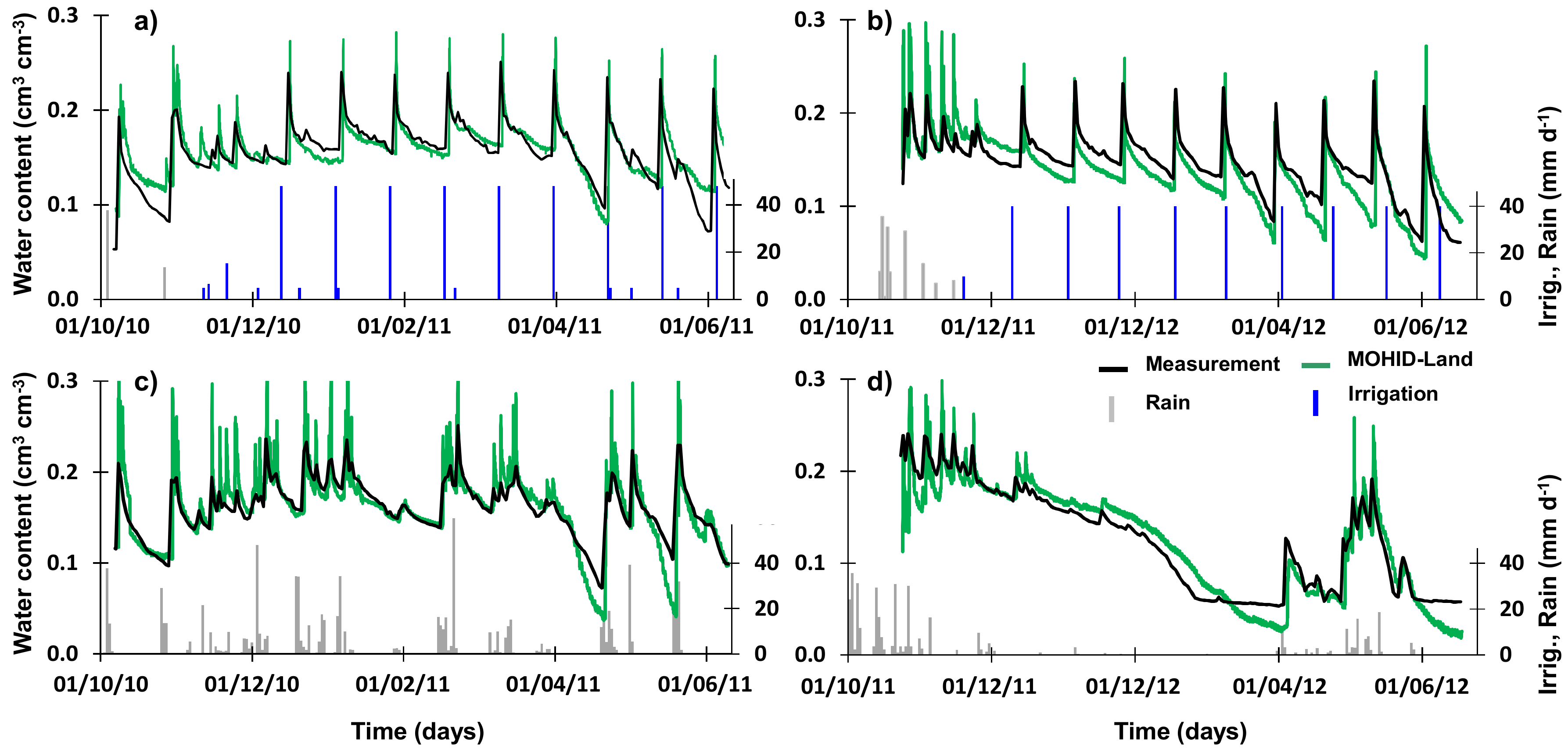
3.1. Soil Water Contents

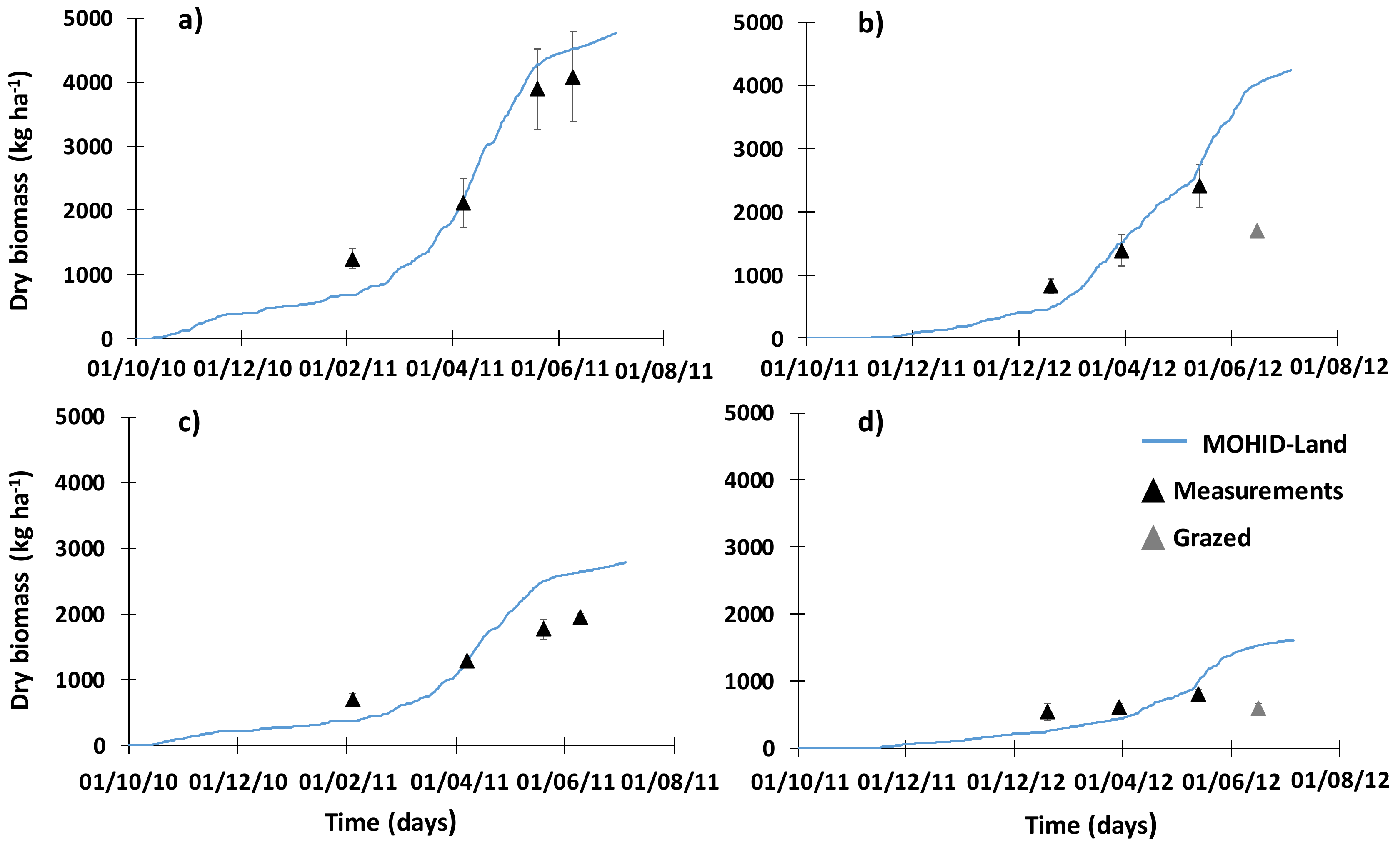
Figure 2 presents the half-hourly θ measurements at 10 cm depth, and compares these values with the MOHID-Land model simulations during the 2010–2011 and 2011–2012 seasons. In the irrigated plots, θ showed a fast increase after rain or irrigation events, then decreased gradually due to redistribution, root water uptake, and soil evaporation. In the rainfed plots, soil water dynamics showed a similar behavior as in the irrigated plots. However, while θ was kept close to field capacity in the 2010–2011 season due to rainfall, in the 2011–2012 season θ was much lower, mainly due to the extended drought period that lasted from December 2011 to March 2012.

Table 4. Results of the statistical analysis of measured and simulated soil water content and aboveground dry biomass.

Statistic	Irrigated Plot		Rainfed Plot
	Water Content (cm3 cm−3)	Aboveground Dry Biomass (kg ha−1)	Water Content (cm3 cm−3)	Aboveground Dry Biomass (kg ha−1)
Calibration set (2010–2011)
ME	0.001	−870.8	−0.002	−739.4
RMSE	0.015	1286.5	0.018	1125.5
NRMSE	0.039	0.210	0.030	0.372
EF	0.632	0.869	0.780	0.584
Validation set (2011–2012)
ME	−0.010	−667.6	−0.003	120.9
RMSE	0.026	1088.1	0.022	279.8
NRMSE	0.047	0.375	0.024	0.243
EF	0.481	0.718	0.863	0.882

ME, mean error; RMSE, root mean square error; NRMSE, normalized RMSE; EF, model efficiency.

presents the statistical indicators obtained after comparing measured values and model simulations. During calibration (2010–2011), the error of the estimates was small, producing an RMSE value of 0.018 and 0.015 cm³ cm⁻³ and an NRMSE value of 0.030 and 0.039 for the rainfed and irrigated plots, respectively, while model efficiency was high (0.632–20.780). For the validation period (2011–2012), the errors of the estimates were kept small (0.22 ≤ RMSE ≤ 0.26 cm³ cm⁻³; 0.024 ≤ NRMSE ≤ 0.047), while the model efficiency was high (0.481 ≤ EF ≤ 0.863). According to Ramos et al. [48], Dabach et al. [49], and Sándor et al. [50], the deviation between measurements and model predictions may be attributed to several reasons, including model inputs, model structure, and field measurement errors, which can be considered also in this study. Nonetheless, the goodness-of-fit indicators were within the range of values reported in the literature for water content simulations using different process-based models [36,51,52,53,54].

3.2. Pasture Growth

Pasture growth parameters were calibrated/validated for the irrigated and rainfed plots separately, based on the observed dynamics under the different regimes. However, only two parameters differed between the irrigation and rainfed regimes (Table 3): the fraction of PHU to reach the end of the canopy development stage (fr_PHU,dev), and the fraction of LAI_max at the end of the canopy development stage (fr_LAImax,dev). These parameters influenced the time needed for pasture to reach the mid-season stage, with irrigated pasture reaching it faster due to higher water availability, and also presenting a higher LAI value at the beginning of that stage (i.e., higher transpiration rates).

Regarding the aboveground dry biomass, the MOHID-Land simulations were in agreement with the measured values (Figure 3; Table 4). For the calibration period, the RMSE values were 1286.5 and 1125.5 kg ha⁻¹ in the irrigated and rainfed plots, respectively. The NRMSE values were 0.210 and 0.372, and model efficiency were 0.584 and 0.869. For the validation period, RMSE, NRMSE, and EF values were within the same order of magnitude of those values.

The general agreement between the simulated and measured data suggested that the calibrated parameters resulted in an adequate estimate of θ and aboveground dry biomass for both the calibration and validation seasons. Thus, it can be concluded that the model performance was generally good, and the model was properly calibrated for simulating soil water dynamics and crop growth in Herdade da Machoqueira do Grou.

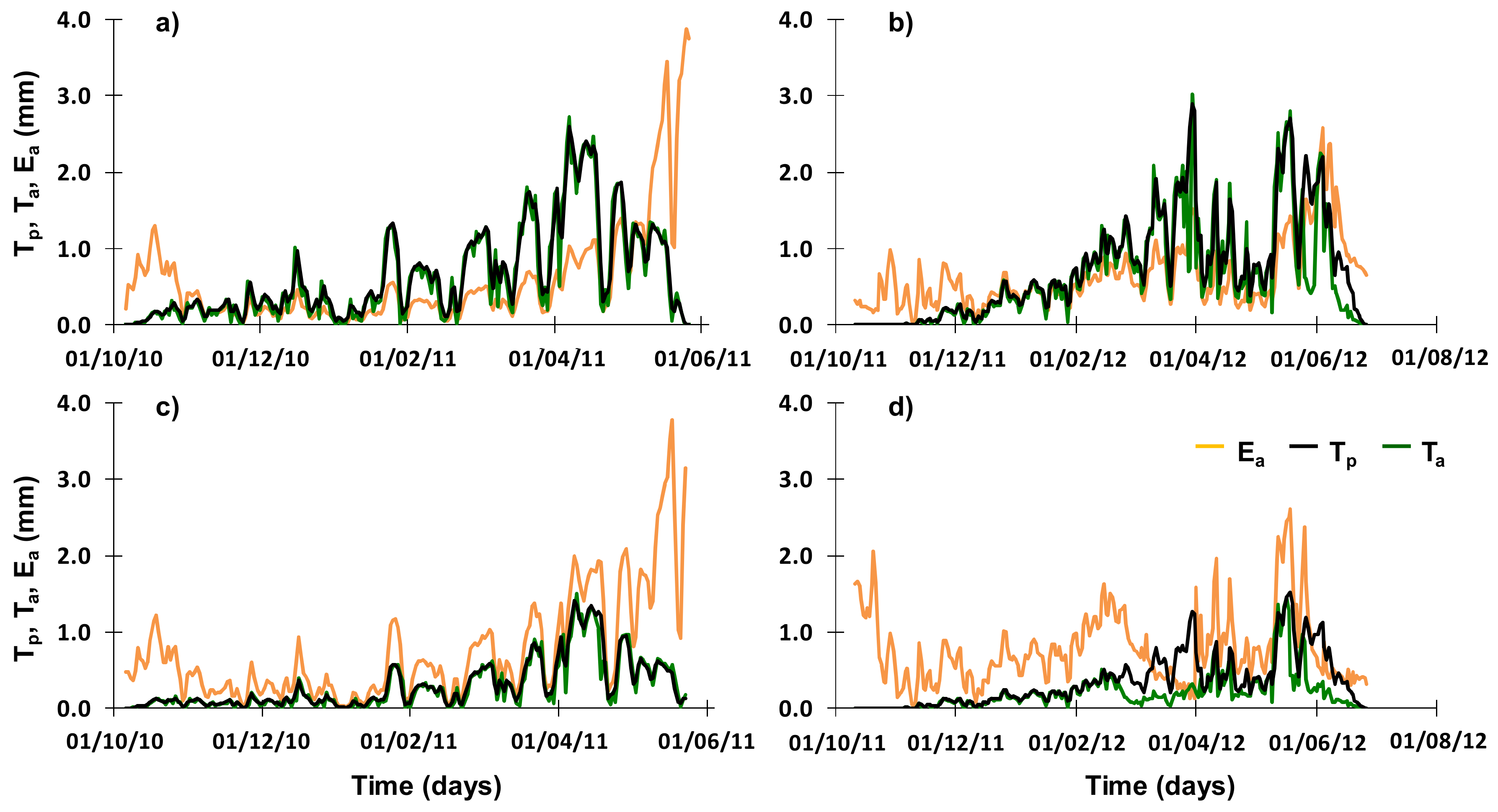
3.3. Soil Water Balance

Table 5. Components of the simulated soil water balance.

Season	Inputs			Outputs
	P (mm)	I (mm)	ΔSS (mm)	Ea (mm)	Ta (mm)	Ta/Tp (-)	DP (mm)
Irrigated plot:
2010–2011	134	454	−31	128	143	0.95	296
2011–2012	152	370	56	155	166	0.86	257
Rainfed plot:
2010–2011	873	0	−263	182	65	0.94	362
2011–2012	413	0	65	198	53	0.60	226

P, precipitation; I, irrigation; E_a, actual soil evaporation; T_a, actual crop transpiration; T_p, potential. crop transpiration; DP, deep percolation; ΔSS, soil moisture variation.

presents the water balance for the irrigated and rainfed plots during the 2010–2011 and 2011–2012 seasons. Precipitation varied considerably between seasons, amounting to 873 mm during the 2010–2011 season and 413 mm during the 2011–2012 season, constituting the sole water input in the rainfed plots. The irrigated plots received natural precipitation until mid-November during the earlier plant stages (134 mm in 2010 and 152 mm in 2011). From that date on, plots were sheltered from rainfall, and an additional 370–454 mm were applied as irrigation [13,14] (Figure 2).

Figure 4 shows the evolution of the T_p, T_a, and E_a values in the irrigated and rainfed plots during the 2010–2011 and 2011–2012 seasons. T_a varied between 143–166 mm in the irrigated plots, and between 56–65 mm in the rainfed plots (Table 5). These values corresponded to a water stress (given by the T_a/T_p ratio) between 0.86–0.95 in the irrigated plots, and between 0.60–0.94 in the rainfed plots. The largest water stress was obviously registered in the rainfed plot during the 2011–2012 season due to the extended drought period observed between December 2011 and March 2012. The E_a values varied between 128–155 mm in the irrigated plots, and between 182–198 mm in the rainfed plots. E_a values were thus notoriously higher than T_a values in the rainfed plots. As discussed by Allen et al. [55], when revising the various methods for field ET estimation, combined approaches of accurate θ observations and water balance simulation modeling provide for appropriate accuracy in ET estimates. Nonetheless, those results are further consistent with Huxman et al. [56] and Kurc and Small [57], who referred to the fact that in semi-arid ecosystems E_a may account for more than half of ET due to the near-surface source of E (the top 20 cm), and because small rainstorms only wet the top few cm of soil. Also, Graham et al. [58] reported pasture losing more water to soil evaporation when compared to ryegrass.

As the rainfall manipulation experiments were carried out between autumn and spring, most of the water applied was lost through deep percolation (226–362 mm), which was to be expected (Table 5), providing natural recharge to the existing aquifers.

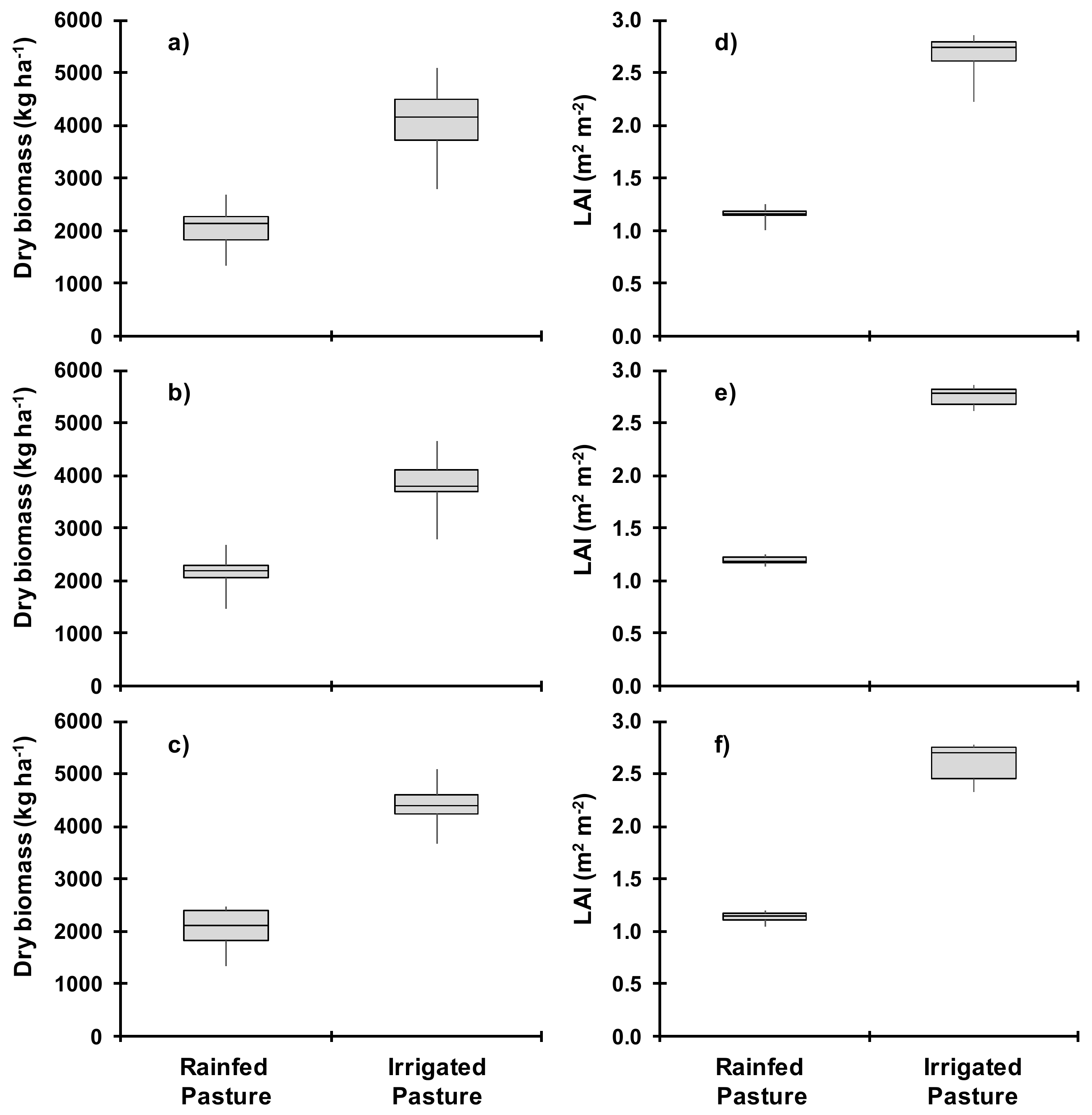
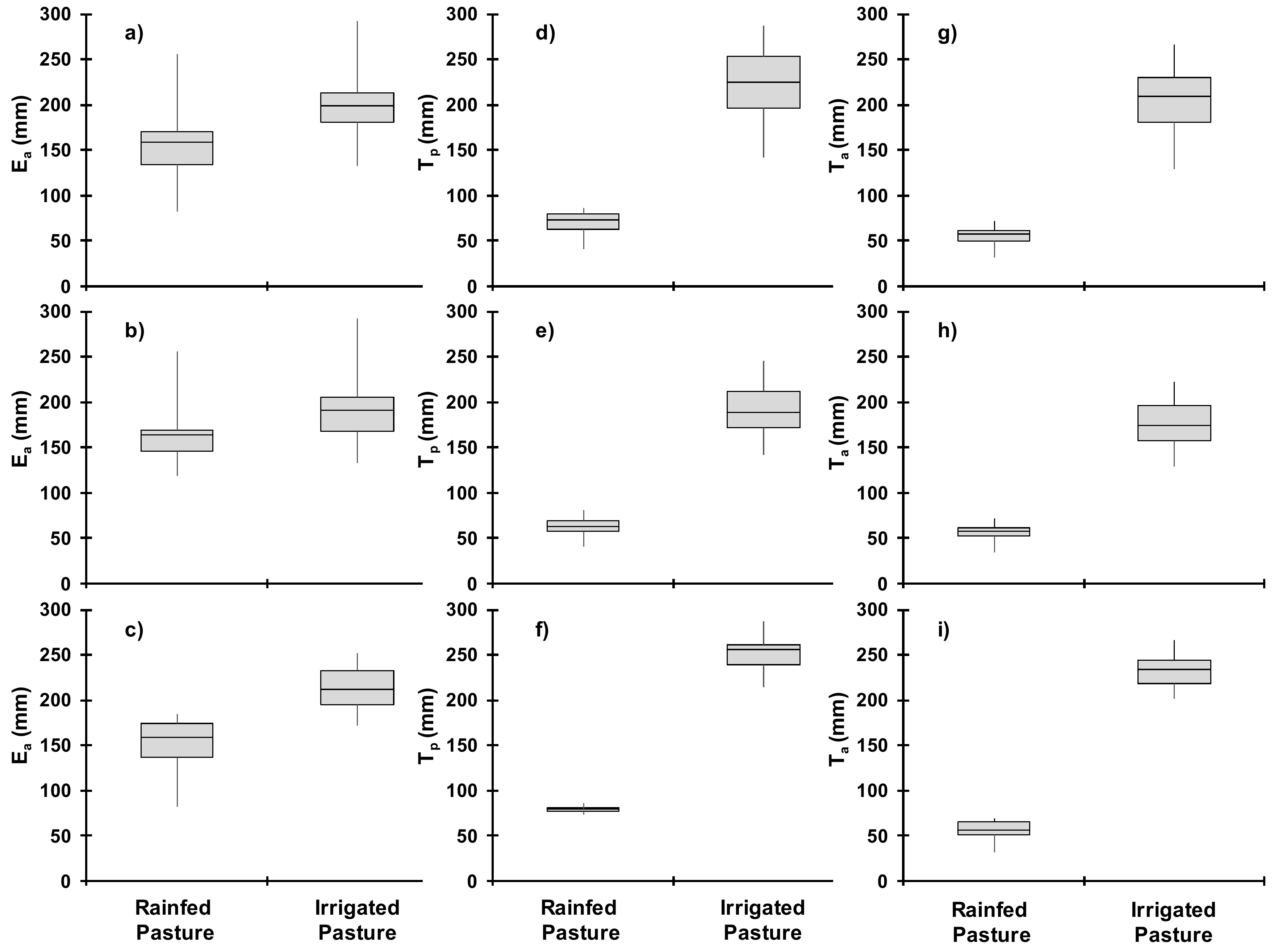
3.4. Dry Biomass and Water Balance Estimates in Wet and Dry Seasons

Model estimates of aboveground dry biomass ranged from 1331 to 2681 kg ha⁻¹ and from 2778 to 5092 kg ha⁻¹ in rainfed and irrigated pasture, respectively, for the period 1979–2009 (Figure 5). Mean differences between the two pasture regimes were found to be statistically different. Likewise, model estimates of the aboveground dry biomass for the 10 driest and the 10 wettest seasons were found to be statistically different. Mean values reached 2055 (1340–2469) and 4395 (3675–5092) kg ha⁻¹ in the rainfed and irrigated regimes, respectively, during the 10 driest seasons, and 2132 (1476–2681) and 3802 (2778–4653) kg ha⁻¹ in the same regimes during the 10 wettest seasons (Figure 5). While mean values in the rainfed regime were relatively close, dry biomass estimates during the wet seasons were more regular, with the first (2067 kg ha⁻¹) and third (2293 kg ha⁻¹) quartiles being relatively close when compared with the dry seasons (Figure 5). Note that simulations of dry biomass values started to differ between pasture regimes during spring, when water became a limiting factor (Figure 3). In these simulations, and based on the field data used for calibrating the model, irrigated pasture was modelled only until June/July, when plants reached their PHU. Therefore, pastures with longer life cycles—namely permanently irrigated pastures—will reach higher dry biomass values, since they are not limited by temperature and water stresses during spring and summer months.

Irrigation was thus a determining factor for pasture’s dry biomass increase. Irrigation needs varied between 20 and 360 mm, being higher during the dry seasons (220–360 mm) than during the wet seasons (20–200 mm). Irrigation needs were obviously dependent of rainfall (R² = 0.513), with the model trying to maintain soil water contents within the predefined threshold (h_t) and target (h₀) pressure heads. Figure 6 gives, as an example, the irrigation scheduling estimated by MOHID-Land for the 1980–1981 (P = 220 mm; I = 360 mm), 1995–1996 (P = 805 mm; I = 140 mm), and 2002–2003 (P = 592 mm; I = 20 mm) seasons. Results showed that rainfall amount and distribution had a notorious influence when computing the soil–water balance and irrigation scheduling with MOHID-Land.

T_p values were also found to be statistically different between rainfed and irrigated pastures. The difference was justified by the LAI values found in each pasture regime (Figure 5), these also being statistically different. As explained earlier, LAI (Equations (4) and (5)) had direct influence on the partition of ET_c values into E_p and T_p. Similarly, T_a values ranged between 32–73 mm and 128–266 mm in rainfed and irrigated pastures (Figure 7), respectively, indicating a water stress that varied between 0.71–5.88% and 0.47–1.97% in the same plots. Water stress was generally higher during the 10 driest seasons, ranging from 1.42 to 5.88% in rainfed pasture and from 0.54–1.97% in irrigated pasture. During the 10 wettest seasons, these values tended to decrease (0.71–2.44% in rainfed pasture, and 0.55–0.99% in irrigated pasture).

As in model calibration/validation, in rainfed pasture, E_a values were always higher than T_a values (83–256 mm). In irrigated pasture, E_a values (133–293 mm) tended to be more similar to T_a values (128–266 mm) (Figure 7), as plants’ canopy considerably increased with the temperature increase during the final stages of pasture development (spring), covering the soil and decreasing the fraction of the soil surface exposed to radiation. During the wet seasons, E_a values estimated for rainfed (118–156 mm) and irrigated (133–293 mm) pasture were more similar to one another than during the 10 driest seasons when the former decreased (83–185 mm) and the latter increased (172–252 mm).

3.5. Future Research Needs Direction

Although the MOHID-Land model results were relatively good, the modeling approach followed in this study was relatively simple, presenting still many limitations that need to be considered in future applications while addressing the complexity of the montado ecosystem.

Firstly, there is the need to simulate the carbon and nutrient fluxes, in order to better unveil uncertainties related to whether and when grasslands act as sinks or sources of ecosystem carbon, providing further insight into the effects of stocking pressures on soil quality. The current model formulation already includes a biochemical module to conduct those studies, and will be the focus of future simulations.

Secondly, there is the need to consider grazing removals during growing seasons, as the system should be seen as dynamic, and interactions with pasturing herds should always be taken into account in a proper management tool. Managing short-term variability in plant growth is considered to present a greater challenge in grazing systems than in cropping systems, which need to be tackled when developing a proper forecasting tool for accurately assessing daily/weekly pasture production [59]. However, for this study grazing was not considered, as the objective was to show the capability of the MOHID-Land model in simulating the main processes related to soil water dynamics and dry biomass growth in the montado ecosystem.

Thirdly, the model currently considers grasslands as a single species, while in fact they should be treated as a mixture of plants with different strategic properties, as suggested by van der Molen et al. [60]. Thus, the model needs to be able to simulate different species within the same cell domain. This approach also needs to be adopted for modeling the rest of the montado ecosystem, namely the niche located directly beneath the tree canopy, and the inter-relationships between the understory and trees for soil water and nutrients [11]. Only by addressing this will it be possible to further understand the ecosystem decline observed in different regions of the southern Iberian Peninsula over the last few decades [6,7], namely the competition and synergies for water resources and nutrients.

Lastly, the MOHID-Land model is a process-based model that simulates variably saturated water flow using the Richards equation. This means that model simulations require reliable information on soil hydraulic properties for computing water flows, which are usually not easily available, as direct measurements are expensive, difficult, and time-consuming [61]. While there is the need to adopt indirect approaches, including pedotransfer functions [62], in order to provide the necessary inputs to process-based models, the approach followed in this study seems preferable to any of the existing simplifications, including those adopted by water-balance models. For example, Sándor et al. [50] compared nine simulation models for predicting θ in the topsoil and biomass production. These authors found that some of the main drivers and results of the grassland processes, particularly θ and yield, were not represented well by common grassland models, attributing deviations between observations and simulations to model formulations rather than structural uncertainties within the models.

4. Conclusions

The MOHID-Land model was able to successfully simulate soil water dynamics and pasture development in a plot located in southern Alentejo, Portugal. Model estimates of θ and aboveground dry biomass showed a general good agreement with field data collected during the 2010–2011 and 2011–2012 seasons. The RMSE, NRMSE, and model efficiency values were lower than 0.026 cm³ cm⁻³, lower than 0.047 cm³ cm⁻³, and higher than 0.481 cm³ cm⁻³ for θ, respectively, and lower than 1286.5 kg ha⁻¹, lower than 0.450, and higher than 0.60 for the aboveground dry biomass. The MOHID-Land model was further shown to take into account climate variability when estimating the soil water balance and biomass growth in two different pasture regimes (rainfed and irrigated). Irrigation played a decisive role in the production of dry biomass, with irrigation amounts varying between 20 and 360 mm. As a result, actual transpiration values (128–266 mm) increased considerably when compared with the corresponding values estimated for rainfed pasture (32–73 mm), being closer to the actual evaporation values observed in both regimes (83–256 mm in rainfed pasture; 133–293 mm in irrigated pasture). However, the higher actual evaporation values show the inefficiency of the system, where most soil water is consumed through a non-beneficial use instead of being converted into biomass.

As precise quantification of water fluxes over the montado ecosystem is essential for accurately quantifying ecosystem carbon and assessing uncertainties related to the source or sink behavior of pastures, the MOHID-Land model can be considered as a valuable tool for farmers to take the stocking rates into account and reduce the adverse impact of grazing in the montado ecosystem.

References

1. Aronson, J.; Santos-Pereira, J.; Pausas, J.G. (Eds.) Cork Oak Woodlands on the Edge: Ecology, Adaptive Management, and Restoration; Island Press: Washington, DC, USA, 2009; pp. 1–10. [Google Scholar]
2. Pinto-Correia, T.; Ribeiro, N.; Sá-Sousa, P. Introducing the montado, the cork and holm oak agroforestry system of Southern Portugal. Agrofor. Syst. 2011, 82, 99–104. [Google Scholar] [CrossRef]
3. Pinto-Correia, T.; Mascarenhas, J. Contribution to the extensification/intensification debate: New trends in the Portuguese montado. Landsc. Urban Plan. 1999, 46, 125–131. [Google Scholar] [CrossRef]
4. Santos, R.; Clemente, P.; Brouwer, R.; Antunes, P.; Pinto, R. Landowner preferences for agri-environmental agreements to conserve the montado ecosystem in Portugal. Ecol. Econ. 2015, 118, 159–167. [Google Scholar] [CrossRef]
5. Guerra, C.A.; Pinto-Correia, T. Linking farm management and ecosystem service provision: Challenges and opportunities for soil erosion prevention in Mediterranean silvo-pastoral systems. Land Use Policy 2016, 51, 54–65. [Google Scholar] [CrossRef]
6. Garrido, P.; Elbakidze, M.; Angelstam, P.; Plieninger, T.; Pulido, F.; Moreno, G. Stakeholder perspectives of wood-pasture ecosystem services: A case study from Iberian dehesas. Land Use Policy 2017, 60, 324–333. [Google Scholar] [CrossRef]
7. Pinto-Correia, T.; Azeda, C. Public policies creating tensions in Montado management models: Insights from farmers’ representations. Land Use Policy 2017, 64, 76–82. [Google Scholar] [CrossRef]
8. Fragoso, R.; Marques, C.; Lucas, M.R.; Martins, M.B.; Jorge, R. The economic effects of common agricultural policy on Mediterranean montado/dehesa ecosystem. J. Policy Model. 2011, 33, 311–327. [Google Scholar] [CrossRef]
9. Sándor, R.; Barcza, Z.; Hidy, D.; Lellei-Kovács, E.; Ma, S.; Bellocchi, G. Modelling of grassland fluxes in Europe: Evaluation of two biogeochemical models. Agric. Ecosyst. Environ. 2016, 215, 1–19. [Google Scholar] [CrossRef]
10. Tenhunen, J.D.; Serra, A.S.; Harley, P.C.; Dougherty, R.L.; Reynolds, J.F. Factors influencing carbon fixation and water use by mediterranean sclerophyll shrubs during summer drought. Oecologia 1990, 82, 381–393. [Google Scholar] [CrossRef] [PubMed]
11. Hussain, M.Z.; Otieno, D.O.; Mirzae, H.; Li, Y.L.; Schmidt, M.W.T.; Siebke, L.; Tenhunen, J.D. CO2 exchange and biomass development of the herbaceous vegetation in the Portuguese montado ecosystem during spring. Agric. Ecosyst. Environ. 2009, 132, 143–152. [Google Scholar] [CrossRef]
12. Jongen, M.; Pereira, J.S.; Aires, L.M.I.; Pio, C.A. The effects of drought and timing of precipitation on the inter-annual variation in ecosystem-atmosphere exchange in a Mediterranean grassland. Agric. For. Meteorol. 2011, 151, 595–606. [Google Scholar] [CrossRef]
13. Jongen, M.; Lecomte, X.; Unger, S.; Pintó-Marijuan, M.; Pereira, J.S. The impact of changes in the timing of precipitation on the herbaceous understorey of Mediterranean evergreen oak woodlands. Agric. For. Meteorol. 2013, 171, 163–173. [Google Scholar] [CrossRef]
14. Jongen, M.; Unger, S.; Fangueiro, D.; Cerasoli, S.; Silva, J.M.N.; Pereira, J.S. Resilience of montado understorey to experimental precipitation variability fails under severe natural drought. Agric. Ecosyst. Environ. 2013, 178, 8–30. [Google Scholar] [CrossRef]
15. Christensen, J.H.; Hewitson, B.; Busuioc, A.; Chen, A.; Gao, X.; Held, I.; Jones, R.; Kolli, R.K.; Kwon, W.-T.; Laprise, R.; et al. Regional climate projections. In Climate Change 2007: The Physical Science Basis; Solomon, S., Qin, D., Manning, M., Chen, Z., Marquis, M., Averyt, K.B., Tignor, M., Miller, H.L., Eds.; Contribution of Working Group I to the Fourth Assessment Report of the Intergovernmental Panel on Climate Change (IPCC); Cambridge University Press: Cambridge, UK, 2007; pp. 847–940. [Google Scholar]
16. IPCC. Climate Change 2007: The Physical Science Basis; Contribution of Working Group I to the Fourth Assessment Report of the Intergovernmental Panel on Climate Change; Cambridge University Press: Cambridge, UK, 2007. [Google Scholar]
17. White, M.A.; Thornton, P.E.; Running, S.W.; Nemani, R.R. Parameterization and Sensitivity Analysis of the BIOME–BGC Terrestrial Ecosystem Model: Net Primary Production Controls. Earth Interact. 2000, 4, 1–85. [Google Scholar] [CrossRef]
18. Brisson, N.; Gary, C.; Justes, E.; Roche, R.; Mary, B.; Ripoche, D.; Sinoquet, H. An overview of the crop model STICS. Eur. J. Agron. 2003, 18, 309–332. [Google Scholar] [CrossRef]
19. Wu, L.; McGechan, M.B.; McRoberts, N.; Baddeley, J.A.; Watson, C.A. SPACSYS: Integration of a 3D root architecture component to carbon, nitrogen and water cycling—Model description. Ecol. Model. 2007, 200, 343–359. [Google Scholar] [CrossRef]
20. Williams, J.R.; Izaurralde, R.C.; Steglich, E.M. Agricultural Policy/Environmental eXtender Model: Theoretical Documentation Version 0604; Texas AgriLIFE Research, Texas A & M University: Temple, TX, USA, 2008; Available online: http://epicapex.brc.tamus.edu (accessed on 15 January 2018).
21. Perego, A.; Giussani, A.; Sanna, M.; Fumagalli, M.; Carozzi, M.; Alfieri, L.; Brenna, S.; Acutis, M. The ARMOSA simulation crop model: Overall features, calibration and validation results. Ital. J. Agrometeorol. 2013, 18, 23–38. [Google Scholar]
22. Ma, S.; Lardy, R.; Graux, A.-I.; Ben Touhami, H.; Klumpp, K.; Martin, R.; Bellocchi, G. Regional-scale analysis of carbon and water cycles on managed grassland systems. Environ. Model. Softw. 2015, 72, 356–371. [Google Scholar] [CrossRef]
23. Trancoso, A.R.; Braunschweig, F.; Chambel Leitão, P.; Obermann, M.; Neves, R. An advanced modelling tool for simulating complex river systems. Sci. Total Environ. 2009, 407, 3004–3016. [Google Scholar] [CrossRef] [PubMed]
24. FAO. World Reference Base for Soil Resources. A Framework for International Classification, Correlation and Communication; World Soil Resources Report 103; Food and Agriculture Organization of the United Nations: Rome, Italy, 2006. [Google Scholar]
25. Soil Survey Staff. Soil Survey Laboratory Information Manual; Soil Survey Investigations Report No. 45; Version 2.0.; Burt, R., Ed.; U.S. Department of Agriculture, Natural Resources Conservation Service: Washington, DC, USA, 2011. [Google Scholar]
26. Gomes, M.P.; Silva, A.A. Um novo diagrama triangular para a classificação básica da textura do solo. Garcia Orta 1962, 10, 171–179. [Google Scholar]
27. Nelson, D.W.; Sommers, L.E. Total carbon, organic carbon, and organic matter. In Methods of Soil Analysis, Part 3. Chemical Methods; Sparks, D.L., Page, A.L., Helmke, P.A., Loeppert, R.H., Soltanpour, P.N., Tabatabai, M.A., Johnston, C.T., Sumner, M.E., Eds.; Soil Science Society of America Inc., American Society of Agronomy Inc.: Madison, WI, USA, 1996; pp. 961–1010. [Google Scholar]
28. Van Genuchten, M.T. A closed-form equation for predicting the hydraulic conductivity of unsaturated soils. Soil Sci. Soc. Am. J. 1980, 44, 892–898. [Google Scholar] [CrossRef]
29. Feddes, R.A.; Kowalik, P.J.; Zaradny, H. Simulation of Field Water Use and Crop Yield; Wiley: Hoboken, NJ, USA, 1978. [Google Scholar]
30. Skaggs, T.H.; van Genuchten, M.T.; Shouse, P.J.; Poss, J.A. Macroscopic approaches to root water uptake as a function of water and salinity stress. Agric. Water Manag. 2006, 86, 140–149. [Google Scholar] [CrossRef]
31. Šimůnek, J.; Hopmans, J.W. Modeling compensated root water and nutrient uptake. Ecol. Model. 2009, 220, 505–521. [Google Scholar] [CrossRef]
32. Allen, R.G.; Pereira, L.S.; Raes, D.; Smith, M. Crop Evapotranspiration—Guidelines for Computing Crop Water Requirements; Irrigation & Drainage Paper 56; FAO: Rome, Italy, 1998. [Google Scholar]
33. Ritchie, J.T. Model for predicting evaporation from a row crop with incomplete cover. Water Resour. Res. 1972, 8, 1204–1213. [Google Scholar] [CrossRef]
34. American Society of Civil Engineers (ASCE). Hydrology Handbook Task Committee on Hydrology Handbook; II Series, GB 661.2. H93; ASCE: Reston, VA, USA, 1996; pp. 96–104. [Google Scholar]
35. Neitsch, S.L.; Arnold, J.G.; Kiniry, J.R.; Williams, J.R. Soil and Water Assessment Tool; Theoretical Documentation; Version 2009; Texas Water Resources Institute; Technical Report No. 406; Texas A&M University System: College Station, TX, USA, 2011. [Google Scholar]
36. Ramos, T.B.; Simionesei, L.; Jauch, E.; Almeida, C.; Neves, R. Modelling soil water and maize growth dynamics influenced by shallow groundwater conditions in the Sorraia Valley region, Portugal. Agric. Water Manag. 2017, 185, 27–42. [Google Scholar] [CrossRef]
37. Monsi, M.; Saeki, T. Uber den Lictfaktor in den Pflanzengesellschaften und sein Bedeutung fur die Stoffproduktion. Jpn. J. Bot. 1953, 14, 22–52. [Google Scholar]
38. Stockle, C.O.; Williams, J.R.; Rosenberg, N.J.; Jones, C.A. A method for estimating the direct and climatic effects of rising atmospheric carbon dioxide on growth and yield of crops: Part I—Modification of the EPIC model for climate change analysis. Agric. Syst. 1992, 38, 225–238. [Google Scholar] [CrossRef]
39. Jones, C.A. C-4 Grasses and Cereals; John Wiley & Sons: New York, NY, USA, 1985; p. 419. [Google Scholar]
40. Purser, R.J.; Leslie, L.M. A Semi-Implicit, Semi-Lagrangian Finite-Difference Scheme Using Hligh-Order Spatial Differencing on a Nonstaggered Grid. Mon. Weather Rev. 1988, 116, 2069–2080. [Google Scholar] [CrossRef]
41. Wesseling, J.G.; Elbers, J.A.; Kabat, P.; van den Broek, B.J. SWATRE: Instructions for Input Report; Winand Staring Centre: Wageningen, The Netherlands, 1991. [Google Scholar]
42. Carsel, R.F.; Parrish, R.S. Developing joint probability distributions of soil water retention characteristics. Water Resour. Res. 1988, 24, 755–769. [Google Scholar] [CrossRef]
43. Mualem, Y. A new model for predicting the hydraulic conductivity of unsaturated porous media. Water Resour. Res. 1976, 12, 513–522. [Google Scholar] [CrossRef]
44. Legates, D.R.; McCabe, G.J. Evaluating the use of “goodness-of-fit” measures in hydrologic and hydroclimatic model validation. Water Resour Res. 1999, 35, 233–241. [Google Scholar] [CrossRef]
45. Moriasi, D.N.; Arnold, J.G.; van Liew, M.W.; Bingner, R.L.; Harmel, R.D.; Veith, T.L. Model Evaluation Guidelines for Systematic Quantification of Accuracy in Watershed Simulations. Transaction of the ASABE: St. Joseph, MI, USA, 2007; Volume 50, pp. 885–900. [Google Scholar]
46. Wang, X.; Williams, J.R.; Gassman, P.W.; Baffaut, C.; Izaurralde, R.C.; Jeong, J.; Kiniry, J.R. EPIC and APEX: Model Use, Calibration, and Validation; Transaction of the ASABE: St. Joseph, MI, USA, 2012; Volume 55, pp. 1447–1462. [Google Scholar]
47. Nash, J.E.; Sutcliffe, J.V. River flow forecasting through conceptual models part I—A discussion of principles. J. Hydrol. 1970, 10, 282–290. [Google Scholar] [CrossRef]
48. Ramos, T.B.; Šimůnek, J.; Gonçalves, M.C.; Martins, J.C.; Prazeres, A.; Pereira, L.S. Two-dimensional modeling of water and nitrogen fate from sweet sorghum irrigated with fresh and blended saline waters. Agric. Water Manag. 2012, 111, 87–104. [Google Scholar] [CrossRef]
49. Dabach, S.; Lazarovitch, N.; Šimůnek, J.; Shani, U. Numerical investigation of irrigation scheduling based on soil water status. Irrig. Sci. 2013, 31, 27–36. [Google Scholar] [CrossRef]
50. Sándor, R.; Barcza, Z.; Acutis, M.; Doro, L.; Hidy, D.; Köchy, M.; Bellocchi, G. Multi-model simulation of soil temperature, soil water content and biomass in Euro-Mediterranean grasslands: Uncertainties and ensemble performance. Eur. J. Agron. 2017, 88, 22–40. [Google Scholar] [CrossRef]
51. Yu, Q.; Saseendran, S.A.; Ma, L.; Flerchinger, G.N.; Green, T.R.; Ahuja, L.R. Modeling a wheat–maize double cropping system in China using two plant growth modules in RZWQM. Agric. Syst. 2006, 89, 457–477. [Google Scholar] [CrossRef]
52. Xu, X.; Huang, G.; Sun, C.; Pereira, L.S.; Ramos, T.B.; Huang, Q.; Hao, Y. Assessing the effects of water table depth on water use, soil salinity and wheat yield: Searching for a target depth for irrigated areas in the upper Yellow River basin. Agric. Water Manag. 2013, 125, 46–60. [Google Scholar] [CrossRef]
53. Wang, X.; Huang, G.; Yang, J.; Huang, Q.; Liu, H.; Yu, L. An assessment of irrigation practices: Sprinkler irrigation of winter wheat in the North China Plain. Agric. Water Manag. 2015, 159, 197–208. [Google Scholar] [CrossRef]
54. Hou, L.; Zhou, Y.; Bao, H.; Wenninger, J. Simulation of maize (Zea mays L.) water use with the HYDRUS-1D model in the semi-arid Hailiutu River catchment, Northwest China. Hydrol. Sci. J. 2016, 62, 93–103. [Google Scholar]
55. Allen, R.G.; Pereira, L.S.; Howell, T.A.; Jensen, M.E. Evapotranspiration information reporting; I: Factors governing measurement accuracy. Agric. Water Manag. 2012, 98, 899–920. [Google Scholar] [CrossRef]
56. Huxman, T.E.; Wilcox, B.P.; Breshears, D.D.; Scott, R.L.; Snyder, K.A.; Small, E.E.; Hultine, K.; Pockman, W.T.; Jackson, R.B. Ecohydrological implications of woody plant encroachment. Ecology 2005, 86, 308–319. [Google Scholar] [CrossRef]
57. Kurc, S.A.; Small, E.E. Soil moisture variations and ecosystem-scale fluxes of water and carbon in semiarid grassland and shrubland. Water Resour. Res. 2007, 43. [Google Scholar] [CrossRef]
58. Graham, S.L.; Kochendorfer, J.; McMillan, A.M.S.; Duncan, M.J.; Srinivasan, M.S.; Hertzog, G. Effects of agricultural management on measurements, prediction, and partitioning of evapotranspiration in irrigated grasslands. Agric. Water Manag. 2016, 177, 340–347. [Google Scholar] [CrossRef]
59. Chapman, D.F.; Rawnsley, R.P.; Cullen, B.R.; Clark, D.A. Inter-annual variability in pasture herbage accumulation in temperate dairy regions: Causes, consequences, and management tools. In Proceedings of the 22nd International Grassland Congress: Revitalising Grasslands to Sustain Our Communities, Sydney, Australia, 15–19 September 2013; pp. 798–805. [Google Scholar]
60. Van der Molen, M.K.; Dolman, A.J.; Ciais, P.; Eglin, T.; Gobron, N.; Law, B.E.; Wang, G. Drought and ecosystem carbon cycling. Agric. For. Meteorol. 2011, 151, 765–773. [Google Scholar] [CrossRef]
61. Dane, J.J.; Topp, G.C. (Eds.) Methods of Soil Analysis Part 4. Physical Methods; Soil Science Society of America, Inc.: Madison, WI, USA, 2002. [Google Scholar]
62. Ramos, T.B.; Gonçalves, M.C.; Brito, D.; Martins, J.C.; Pereira, L.S. Development of class pedotransfer functions for integrating water retention properties into Portuguese soil maps. Soil Res. 2013, 51, 262–277. [Google Scholar] [CrossRef]
Figure 1. Annual precipitation and reference evapotranspiration (ET0) between the 1979–980 and 2007–2008 seasons.
Water 10 00489 g001
Figure 2. Measured and simulated soil water contents at 10 and 5 cm depth in irrigated and rainfed plots, respectively: (a) irrigated plot during the 2010–2011 season; (b) irrigated plot during the 2011–2012 season; (c) rainfed plot during the 2010–2011 season; and (d) rainfed plot during the 2011–2012 season.
Water 10 00489 g002
Figure 3. Measured and simulated aboveground dry biomass in irrigated and rainfed plots. (a) irrigated plot during the 2010–2011 season; (b) irrigated plot during the 2011–2012 season; (c) rainfed plot during the 2010–2011 season; and (d) rainfed plot during the 2011–2012 season (marks in grey were not considered in the statistical analysis as measurements showed that sites were grazed).
Water 10 00489 g003
Figure 4. Estimates of water fluxes in irrigated and rainfed plots: (a) irrigated plot during the 2010–2011 season; (b) irrigated plot during the 2011–2012 season; (c) rainfed plot during the 2010–2011 season; and (d) rainfed plot during the 2011–2012 season.
Water 10 00489 g004
Figure 5. Aboveground dry biomass and leaf area index (LAI) values estimated in rainfed and irrigated pastures between the 1979–1980 and 2007–2008 seasons: (a,d) average years; (b,e) 10 wettest years; and (c,f) 10 driest years.
Water 10 00489 g005
Figure 6. Seasonal variation of actual evaporation (Ea), potential transpiration (Tp), and actual transpiration (Ea) values during the 1980–1981 (a), 1995–1996 (b), and 2002–2003 (c) seasons.
Water 10 00489 g006
Figure 7. Actual evaporation (Ea), potential transpiration (Tp), and actual transpiration (Ea) values estimated in rainfed and irrigated pastures between the 1979–1980 and 2007–2008 seasons: (a,d,g) average years; (b,e,h) 10 wettest years; and (c,f,i) 10 driest years.
Water 10 00489 g007