Article

A Fuzzy Max–Min Decision Bi-Level Fuzzy Programming Model for Water Resources Optimization Allocation under Uncertainty

1
Key Laboratory of Subsurface Hydrology and Ecological Effect in Arid Region, Ministry of Education, Chang’an University, Xi’an 710054, China
2
School of Environmental Science and Engineering, Chang’an University, Xi’an 710054, China
*
Author to whom correspondence should be addressed.
Water 2018, 10(4), 488; https://doi.org/10.3390/w10040488
Submission received: 14 March 2018 / Revised: 3 April 2018 / Accepted: 11 April 2018 / Published: 16 April 2018
(This article belongs to the Section Urban Water Management)

Abstract

:
Water competing conflict among water competing sectors from different levels should be taken under consideration during the optimization allocation of water resources. Furthermore, uncertainties are inevitable in the optimization allocation of water resources. In order to deal with the above problems, this study developed a fuzzy max–min decision bi-level fuzzy programming model. The developed model was then applied to a case study in Wuwei, Gansu Province, China. In this study, the net benefit and yield were regarded as the upper-level and lower-level objectives, respectively. Optimal water resource plans were obtained under different possibility levels of fuzzy parameters, which could deal with water competing conflict between the upper level and the lower level effectively. The obtained results are expected to make great contribution in helping local decision-makers to make decisions on dealing with the water competing conflict between the upper and lower level and the optimal use of water resources under uncertainty.

1. Introduction

Water is a fundamental resource and is essential for all forms of life, and has benefited people and their socioeconomics for many centuries. According to the United Nations, approximately 700 million people in 43 countries are suffering from water scarcity, and 1.8 billion people will be living in countries or regions with severe water scarcity by 2025 [1]. Agricultural irrigation, which is the largest consumer of limited water resources, consumes approximately 70% of the world’s freshwater withdrawals, especially in arid and semi-arid areas, which are mainly characterized by low rainfall and high evaporation [2,3]. For example, Huang et al. (2012) indicated that approximately 90% of water consumption was occupied by agricultural irrigation in the arid area of northwest China [4]. The conflict between limited water resources and water demand has become a very serious issue with continuing population growth and rapid development of socioeconomic systems. Furthermore, water competing conflict among water competing sectors has also become more and more serious, especially for water competing sectors from different levels. Therefore, it is desirable for decision-makers to form integrated strategies which not only utilize limited water resources effectively but also deal with the water competing conflict among water competing sectors from different levels.
Optimization of water resources is a potential way to solve the above problems. In the past decades, a number of optimization methods have been proposed for water resources management [5,6,7,8,9,10,11,12,13]. For example, Guo et al. 2010 presented a fuzzy stochastic two-stage programming approach, which offered various policy scenarios with different economic penalties, to water resources management under uncertainty [14]. In order to handle economic expenditure caused by regional water shortage and flood control, an interval parameter multistage joint-probability programming model was developed for water resources management [15]. Li et al. (2015) presented a two-level linear fractional water programming approach, aimed at solving ratio multi-objective problems, to optimize water resources [16]. A multi-objective socioeconomic model, aimed at job creation, was developed for optimal and efficient management of water resources among multi-water sectors [17]. Ren et al. (2016) developed a multi-objective stochastic fractional goal programming model, dealing with economic and social objectives simultaneously and taking water quantity and water quality under consideration, for optimal water resources [18]. However, the above studies have just focused on optimizing water resources allocation in one water sector, such as making maximum benefit/yield, minimum system cost. Even though there were optimal methods for optimization allocation of water resources among multi-water competing sectors, it just focused on solving water competing conflict of multi-water competing sectors at the same level. In general, the above studies could not optimize limited water resources and solve water competing conflict among water competing sectors from different levels.
Therefore, in order to solve these kinds of problems, this paper puts forward bi-level programming (BLP). A BLP model has a hierarchical structure in which an upper-level and a lower-level decision-maker must select their strategies so as to optimize their objective functions, respectively. Further, the upper-level decision-maker knows how the lower-level optimizer would react to a given upper-level decision and acts accordingly, while the lower-level optimizer can act only according to given decisions of an upper-level problem [19]. In this paper, we use the fuzzy max–min decision model for generating Pareto optimal solution [20]. Thus, it presents a fuzzy max–min decision bi-level programming (FMDBLP) model. Compared with the above methods and linear BLP, the FMDBLP model has the following advantages. (1) It can optimize limited water resources and deal with water conflict among water competing sectors simultaneously; (2) It can solve water competing conflict among water competing sectors not only at the same level but also from different levels; (3) It also has the characteristics that deal with programming with linear or nonlinear constraints, especially for dealing with nonlinear objective functions at each level. The proposed FMDBLP model can be used to optimize limited water resources effectively and deal with water competing conflict among water competing sectors from different levels simultaneously.
Furthermore, uncertainties are inevitable in the optimization process, such as crop planting area, groundwater resources, irrigation quota, and economic parameters [21,22]. Therefore, many optimization allocation models under uncertainty were developed to deal with such problems, such as stochastic mathematical programming (SMP) and interval stochastic programming (ISP) [23,24]. In the irrigation systems, a serial of parameters has fuzzy characters, such as irrigation quotas, water resources consumption, and planting areas. Fuzzy sets can be used to better describe vague essences in the phenomena mentioned above by dividing them into different membership grades, which helps to provide flexible management measures for both water authorities and water users. However, there was little research that handled both fuzzy uncertainty and FMDBLP.
Therefore, this study aims at developing FMDBLFP for water resources optimization allocation under uncertainty by coupling fuzzy sets theory with FMDBLP. Optimizing limited water resources and dealing with water competing conflict among water competing sectors under fuzzy uncertainty, which belongs to different levels, are the objectives of the developed model. The proposed model was applied to Wuwei City, Gansu Province, which is located in northwest region of China, and is characterized by low rainfall and high evapotranspiration. A range of water resources optimal allocation plans were provided for the decision-makers. The FMDBLFP model can be used to help decision makers to identify a desired water resource optimal allocation plan for solving water competing conflicts among multi-water competing sectors belonging to different levels under uncertainty.

2. Methodology

2.1. Bi-Level Programming

The general formulation of a BLP problem is as follow [25]:
  • (The upper-level)
    max x X , y F ( x , y ) s . t . G ( x , y ) 0 ,
    where y can be solved from
  • (The lower-level)
    max y f ( x , y ) s . t . g ( x , y ) 0 ,
    where x R n 1 and y R n 2 . The variables of problem (1) are divided into two classes, namely the upper-level variables x R n 1 and the lower-level variables y R n 2 . Similarly, the functions F : R n 1 × R n 2 R and f : R n 1 × R n 2 R are the upper-level and lower-level objective functions, respectively, while the vector-valued functions G : R n 1 × R n 2 R m 1 and g : R n 1 × R n 2 R m 2 are called the upper-level and lower-level constraints, respectively. The upper-level decision-maker (ULDM) controls vector x , and the lower-level decision-maker (LLDM) controls vector y .

2.2. Fuzzy Set Theory

In order to solve a fuzzy problem quantitatively, functions with simple formalism, such as triangle-shape grade membership function and trapezoidal linear function, were often used to reflect the fuzzy concept clearly as membership functions [26]. In this study, we selected the trapezoid linear function as the membership function of BLFWA model, which can reflect more information than the triangle shape grade membership function. The expression for the trapezoidal function can be described as:
μ ( x ) = { 0 x A 1 min   or   x A 2 max x A 1 min A 1 A 1 min A 1 min < x < A 1 A 2 max x A 2 max A 2 A 2 < x < A 2 max 1 A 1 < x < A 2
The illustration of the corresponding variables is shown in Figure 1.
Figure 1 shows the trapezoidal membership function of different α - cut levels. α - cut is the level set, describing the fuzzy degree of membership level perfectly, and is important for a fuzzy event’s quantization. Different α - cut can represent quantitatively different levels of the possibility of events under uncertainty on account of many levels in fuzzy events of water optimal allocation. For example, α = 0 represents the lowest possibility of the occurrence of events, while α = 1 represents the greatest possibility of the occurrence of events. Moreover, different α - cut can reflect the changing trend of the optimal results under different degrees of uncertainty.
Therefore, based on the concept of α - cut , the α - cut level for the trapezoidal fuzzy sets (i.e., A ˜ = ( A 1 min , A 1 , A 2 , A 2 max ) ) can be expressed as closed intervals:
[ ( 1 α ) A 1 min + α A 1 ,   ( 1 α ) A 2 max + α A 2 ]

2.3. Fuzzy Max–Min Decision Bi-Level Programming

The solving steps of FMDBLP are as following:
The ULDM problem
Max F 1 ( x ) s . t . G ( x ) 0
F 1 ( x ) , G ( x ) are the objective function and constraint of the UL, respectively. First, the individual best solution ( F 1 ) and individual worst solution ( F 1 ) of (5) are found, where
F 1 = Max   F 1 ( x ) s . t . G ( x ) 0 ,   F 1 = Min   F 1 ( x ) s . t . G ( x ) 0
This data can then be formulated as the following membership function of fuzzy set theory [27]:
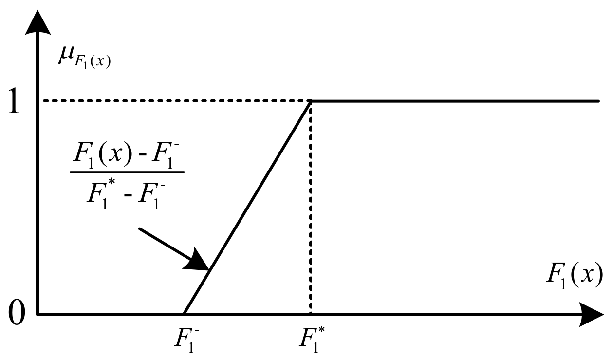
μ [ F 1 ( x ) ] = { 1 if   F 1 ( x ) > F 1 F 1 ( x ) F 1 F 1 F 1 if   F 1 F 1 ( x ) F 1 0 if   F 1 > F 1 ( x )
Figure 2 represents the schematic diagram of Equation. It was as following:
Then, building the following mixed Tchebycheff model based on Equation (7):
Max   λ s . t . μ [ F 1 ( x ) ] λ , λ [ 0 , 1 ] , G ( x ) 0 .
The solution of the ULDM, [ x U , F 1 U , λ U ] can be solved by the model (8).
The LLDM problem
Max F 2 ( x ) s . t . G ( x ) 0
F 2 ( x ) , G ( x ) are the objective function and constraint of the LL, respectively. By the same way of ULDM determination, we can get the solution of the LLDM, [ x L , F 2 L , λ L ] .
FMDBLP problem
The solution of ULDM and LLDM is disclosed above. However, two solutions are usually different due to the nature between two levels of objective functions. Therefore, it is unreasonable to use the optimal decision x 1 H , which is from ULDM, as a control factor for the LLDM. It is more reasonable to have some tolerance that gives the LLDM an extent feasible region to search for its optimal solution.
Therefore, the range of decision variable x 1 should be around x 1 H , with maximum tolerance t 1 and the following membership function specifying x 1 as:
μ ( x 1 ) = { 0 if   x 1 < x 1 H t 1 x 1 ( x 1 H t 1 ) t 1 if   x 1 H t 1 x 1 x 1 H ,   ( x 1 H + t 1 ) x 1 t 1 if   x 1 H x 1 x 1 H + t 1 , 0 if   x 1 x 1 H + t 1 ,
where x 1 H presents the most preferred solution; ( x 1 H t 1 ) and ( x 1 H + t 1 ) are the worst acceptable decision; and that satisfaction is linearly increasing with the interval of [ x 1 H t 1 , x 1 ] and linearly decreasing with [ x 1 , x 1 H + t 1 ] , and other decisions are not acceptable.
Then, the membership function of the HLDM is as follows:
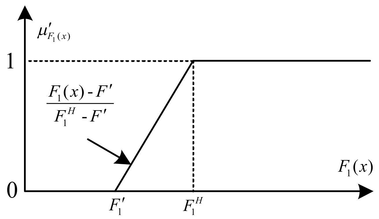
μ [ F 1 ( x ) ] = { 1 if   F 1 ( x ) > F 1 H , F 1 ( x ) F 1 F 1 H F 1 if   F 1 F 1 ( x ) F 1 H , 0 if   F 1 > F 1 ( x ) .
and is presented graphically as follows (Figure 3):
where F 1 H = F 1 ( x H ) , F 1 = F 1 ( x L ) . x L is the solution of LLDM.
The membership function of the LLDM is as following:
μ [ F 2 ( x ) ] = { 1 if   F 2 ( x ) > F 2 L , F 2 ( x ) F 2 F 2 L F 2 if   F 2 F 2 ( x ) F 2 L , 0 if   F 2 > F 2 ( x ) .
Figure 4 represents the schematic diagram of Equation (12). It was as following:
where F 2 L = F 2 ( x L ) , F 2 = F 2 ( x H ) . x H is the solution of ULDM.
Finally, the FMDBLP model can be described as:
Max   δ s . t . x 1 ( x 1 H t 1 ) t 1 δ I , ( x 1 H + t 1 ) x 1 t 1 δ I , μ [ F 1 ( x ) ] δ , μ [ F 2 ( x ) ] δ , δ [ 0 , 1 ] , G ( x ) 0 .
where δ is the overall satisfaction and I is the column vector with all elements equal to 1. By solving model (13), the optimal solution of FMDBLP is reached.

2.4. Fuzzy Max–Min Decision Bi-Level Fuzzy Programming (FMDBLFP)

In order to solve fuzzy problem quantitatively, the trapezoidal linear function, which was an effective solution for fuzzy problems, was introduced into the FMDBLP model. Therefore, the fuzzy max–min decision bi-level fuzzy programming model was developed for solving the bi-level problems with fuzzy problems. The FMDBLFP model can be described as:
  • Upper level
    max F ( x ) = A x + B s . t .     E x + H 0
  • Lower level
    max f ( x ) = C x + D s . t .     E x + H 0
    where A , C , E   and   H denote fuzzy coefficients of the objective and constraints; B and D are crisp numbers constants (fuzzy singletons). The steps of solving the FMDBLFP model are as following:
    • Build original FMDBLFP model [Equations (14) and (15)];
    • Convert the fuzzy coefficients of [Equations (14) and (15)] into the closed intervals as [Equation (6)] by [Equation (5)];
    • Preset the value of α and solve the FMDBLFP model by the solving method [Equations (2) and (3)];
    • Change the value of α and repeat steps 2 and 3;
    • Get the optimal solution under different α levels.

3. Application

3.1. Study Area

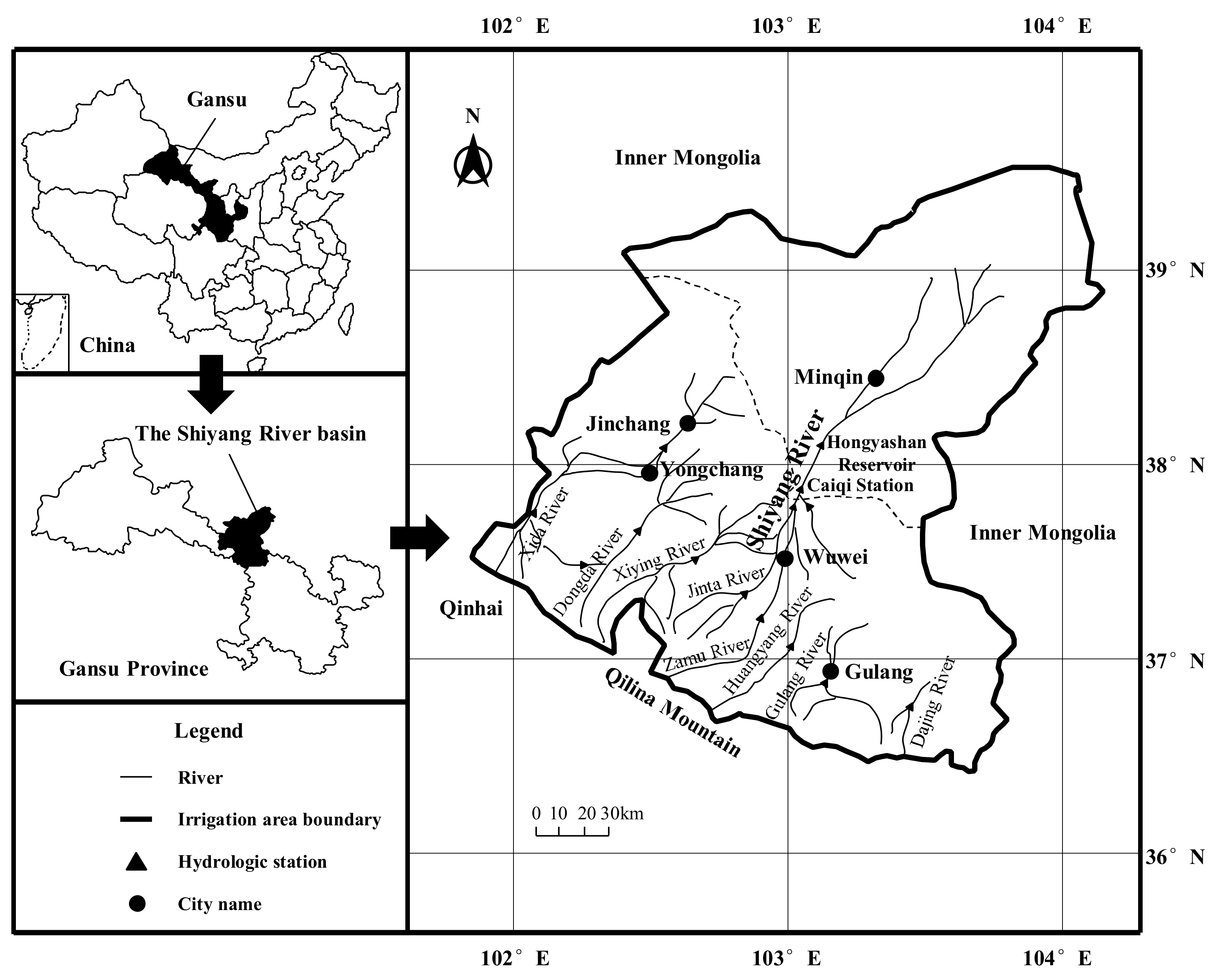
The research area is located in Wuwei City (101°49′–104°16′ E, 36°29′–39°27′ N), Gansu Province, China (Figure 5), located to the north of Qilian Mountain and south of Desert Tenggeli. Wuwei’s annual rainfall is about 60–610 mm and the annual evapotranspiration is about 1400–3040 mm. Wuwei is one of the most arid areas in China, whose main water supply is dependent on Shiyang River and groundwater.
Recently, the water shortage of Wuwei city has become more and more serious due to the slow decrease of river runoff, the policy of protecting ecological environment by restricting groundwater exploitation, and the increase of water demand for repairing the ecological environment in Shiyang downstream. However, irrigation is the largest water consumer and even accounts for about 88.28% of Wuwei’s total water consumption. Thus, the water competing conflict among multi-water competing sectors in Wuwei city for limited water resources becomes more and more serious, especially water competing conflict between irrigation and the rest of water users. Moreover, in order to achieve sustainable development of Wuwei city, the government wants to cut down farmland and irrigation water for saving water resources for other water users, aiming at maximizing the net benefit of the government’s objective. However, the farmers will suffer great losses. Therefore, there is great conflict between the government’s objective (the upper level) and the farmers’ objective (the lower level) about the allocation of limited water resources. Therefore, it is important for the decision-makers to make a water resources allocation plan, which can not only allocate the limited water resources efficiently but also deal with the conflict among water competing sectors from different levels. Considering the possible uncertainties existing in the water resources optimal allocation, this paper established a fuzzy max–min decision bi-level fuzzy optimal allocation model for Wuwei city. This model can allocate water resources efficiently and deal with water competing conflict between the government’s objective (the upper level) and the farmer’s objective (the lower lever), in conjunction with surface and groundwater, food security, and other factors.
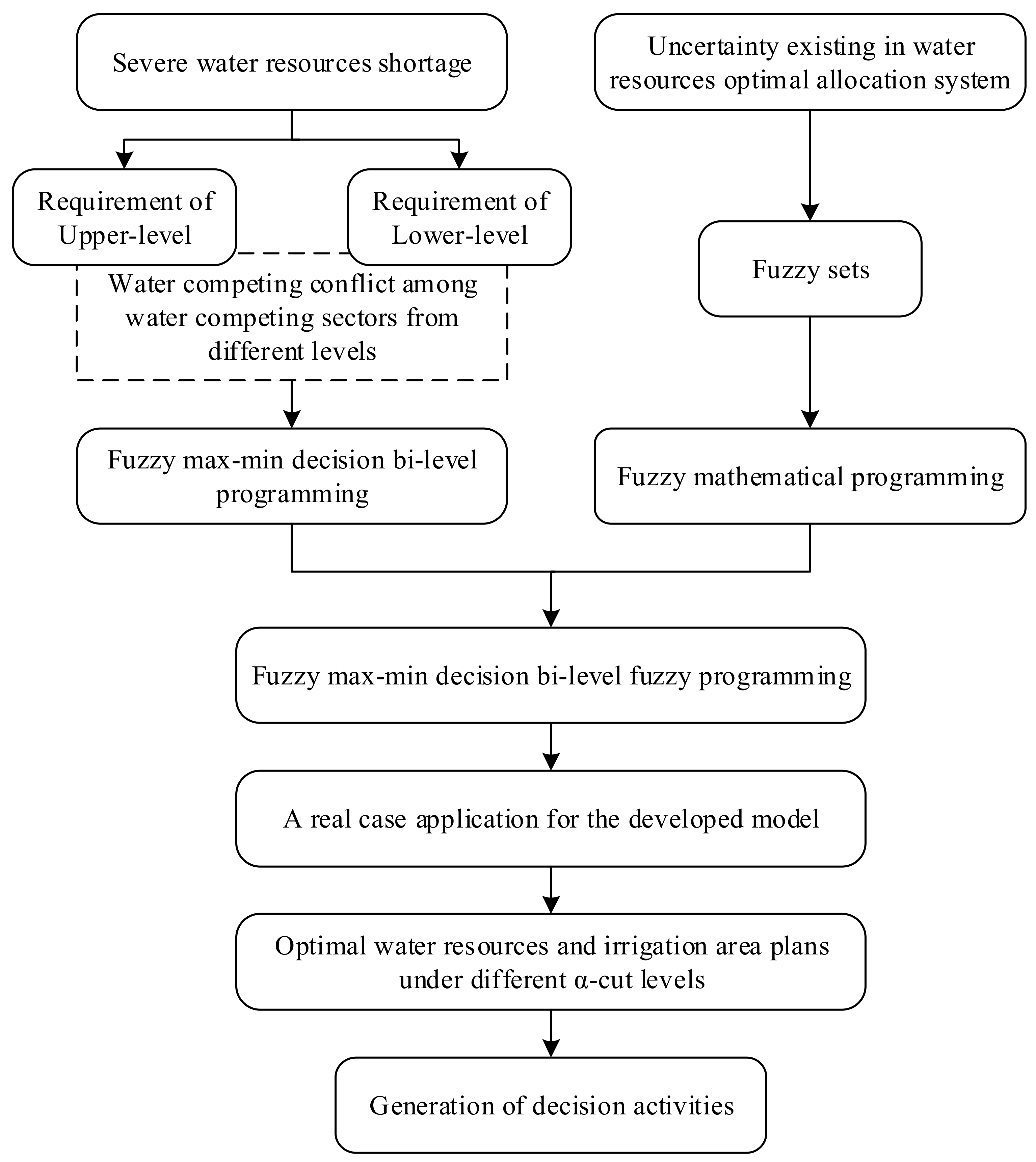
Figure 6 represented the schematic diagram of the developed FMDBLFP model.

3.2. Model Building

The FMDBLFP model for water resources optimization allocation can be described as:
The upper level (the government’s objective)
Max = i = 1 4 ( O i × A i × I i + S i × S W i + T i × T W i )
This represents the objective of the upper level, which is aimed at maximization of economic benefit. Moreover, it reflects the requirement of government.
The lower level (the farmer’s objective)
Max = i = 1 4 B i × A i
This represents the objective of the lower level, which is aimed at the maximization of grain yield. Moreover, it reflects the requirement of the farmers.
Subject to
(Water resources constraints)
i = 1 4 ( I i × A i + S W i + T W i + W D i + W E i ) W
This represents that the total water consumption cannot exceed the maximum available supply of water resources. In addition, the maximum available supply of water resources has a fuzzy characteristic.
A W i min I i × A i A W i max S W i min S W i S W i max T W i min T W i T W i max
This represented that the water consumption of each industry should meet the minimum water requirement and cannot exceed maximum availably supply of water resources.
(Food security constraints)
E P i × L F i B i × A i
This represents that the food demand of each irrigation district should be satisfied in the process of optimization allocation of water resources.
(Farmland constraints)
A i M A i
This represents that the irrigation areas of each irrigation district cannot exceed the maximum available amount of irrigation areas.
The variables are:
  • M A i , A i : Maximum irrigation areas, irrigation areas of region i (104 mŭ); (mŭ is equal to 614.4 m2);
  • E P i : Population of region i (104 p);
  • L F i : Food demand per capita of region i (t/p);
  • I i : Irrigation water of per unit irrigation areas in region i (m3/ mŭ);
  • S W i , T W i : Water supply for the secondary and tertiary industry of region i (104 m3);
  • W D i , W E i : Domestic water and ecological water in region i;
  • O i , S i , T i : Per unit of water resources benefit of planting, secondary and tertiary industry in region i (yuan/m3);
  • B i : Yield per unit of region i (t/ mŭ);
  • W : Water supply for Wuwei City, which is fuzzy sets;
  • A W i min , A W i max : Minimum and maximum water supply for the planting industry of region i (104 m3);
  • S W i min , S W i max : Minimum and maximum water supply for the secondary industry of region i (104 m3);
  • T W i min , T W i max : Minimum and maximum water supply for the tertiary industry of region i (104 m3);
The objective of the above model was attainment of the optimal allocation plans of water resources, and further to optimizing water resources effectively, also can dealing with water competing conflict between government objective (the upper level) and farmer objective (the lower level).
The constraints reflect the relationship between decision variables and water resources allocation clearly. Table 1 shows the maximum irrigation areas (MAi 104 mŭ), yield per unit area (Bi t/mŭ), population (EPi 104 P), food demand per capita (LFi t/p), irrigation water per unit (Ii m3), per unit of water resources benefit of the planting (Oi yuan/m3), secondary and tertiary industry (Si yuan/m3), domestic water demand (WDi 104 m3), and ecological water demand (WEi 104 m3) of the four regions. Table 2 represents the maximum and minimum water supply of the planting industry, the secondary industry, and the tertiary industry. In addition, the water supply of Wuwei City has the characteristic of fuzzy uncertainty. Moreover, it can be represented as trapezoidal fuzzy sets, which are presented as [15.49 × 10⁸, 16.14 × 10⁸, 16.84 × 10⁸, 17.97 × 10⁸] m3.

4. Results and Analysis

4.1. Solution of the FMDBLFP

Table 3 and Table 4 represent the optimal allocation plans of irrigation area and water resources for different irrigation districts under different a - cut levels, which were obtained by the FMDBLFP model. In addition, for the purpose of making the information contained relatively uniform, six a - cut level values were chosen: 0, 0.2, 0.4, 0.6, 0.8, and 1. The results displayed in Table 3 suggest that the irrigation area of each irrigation district would vary under different α - cut levels. Such changes would mainly take place in Liangzhou. In general, the decrease of irrigation areas mainly occurs in the irrigation districts with low unit yields. For example, Liangzhou has the lowest unit yield among four irrigation districts. Table 4 shows the optimal allocation plans of water resources in each irrigation district. The characteristic used was that the land use of each irrigation district would not vary under different α - cut levels. Moreover, it was the same as maximum supply of water resources in the constraint. This was because the economic benefit per unit of water resources is much more than it in the planting industry. Therefore, the demand of secondary and tertiary industry is firstly satisfied with the water demand, and then the rest of water resources are optimally allocated for irrigation.
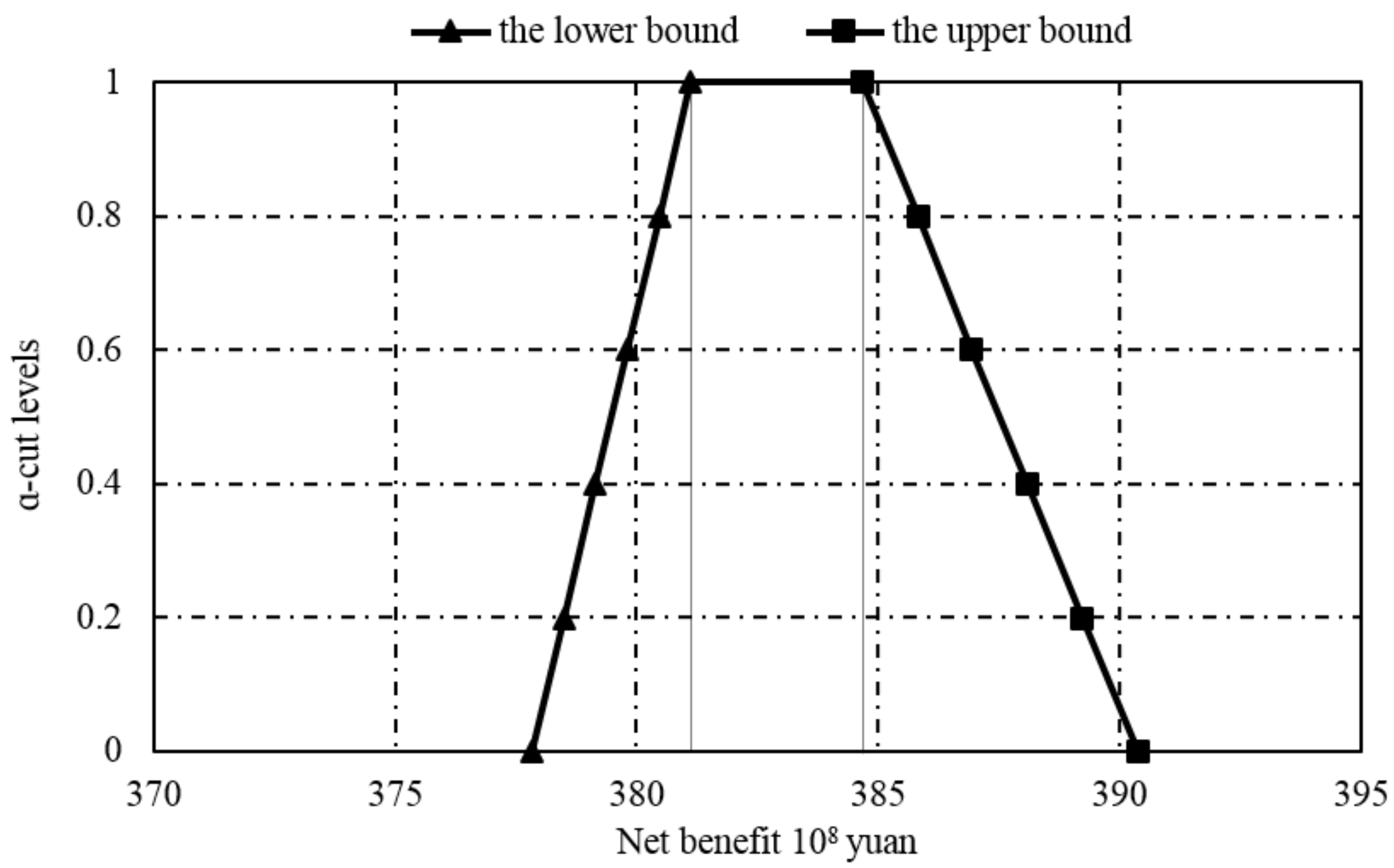
Figure 7 and Figure 8 illustrate the lower- and upper-bound values of yields and net benefits under different α - cut levels. From the figures, as α - cut levels increased, the upper-bound of optimized yields and net benefit decreased, while the lower-bound of optimized yield and net benefit increased. For example, the upper-bound yields would vary from 120.19 × 10⁴ t ( α = 0 ) to 110.24 × 10⁴ t ( α = 1 ). The lower-bound yields would vary from 98.34 × 10⁴ t ( α = 0 ) to 104.07 × 10⁴ t ( α = 1 ). In this paper, trapezoidal function was selected as fuzzy membership functions, which has the characteristic as the larger α - cut levels, the larger the possibility of the occurrence of events shown in Figure 1. As α - cut levels increased, the fuzzification weakens. Therefore, the optimized yields and net economic benefit gap between the upper bound and the lower bound was wide when α = 0 , and narrow when α = 1 . Therefore, different policies might be adopted for water resources allocation and water saving targets under different water resources shortage conditions, thus lead to broad options of varied system objects and system-failure risks.

4.2. Comparison of FMDBLFP with ULDM and LLDM

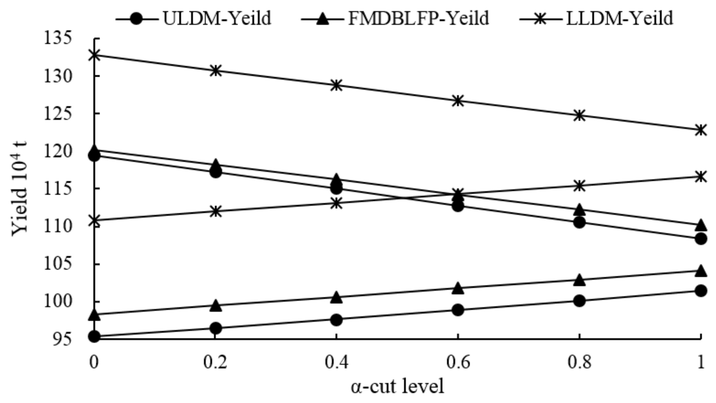
In the process of solving the developed FMDBLFP model, the optimal results of the ULDM and LLDM can be got, which just made upper-level (maximum economic benefits) and lower-level (maximum yields) objectives as the optimization objectives, respectively. Figure 9 and Table 5 represent the optimized yields and optimized net benefits of the developed FMDBLFP, ULDM, and LLDM under different α - cut levels. From the figure and table, the optimized results of the three models had the same tendency under different α - cut levels. As α - cut levels increased, the upper-bound of optimized yields and net benefits decreased, while the lower-bound of yields and net benefits increased. For example, the upper-bound yields of ULDM would vary from 119.47 × 10⁴ t ( α = 0 ) to 108.32 × 10⁴ t ( α = 1 ), while the lower-bound yields of ULDM would vary from 95.32 × 10⁴ t ( α = 0 ) to 101.41 × 10⁴ t ( α = 1 ). However, there were great differences in the optimized yields and net benefits obtained by the three models. From Figure 9, the optimized yield of ULDM was largest under each α - cut level. Furthermore, Table 5 shows that the optimized economic benefit of LLDM was largest under each α - cut level. In addition, regardless of yields or economic benefits, the optimized result of FMDBLFP was always between ULDM and LLDM. For example, the optimized yields of LLDM, FMDBLFP, and ULDM were [114.30 × 10⁴ t, 126.75 × 10⁴ t], [101.78 × 10⁴ t, 114.21 × 10⁴ t], and [98.85 × 10⁴ t, 112.76 × 10⁴ t], respectively, when α = 0.6 . When α = 1 , the optimized economic benefits of ULDM, FMDBLFP, and LLDM were [384.98 × 10⁸ yuan, 381.60 × 10⁸ yuan], [384.67 × 10⁸ yuan, 381.12 × 10⁸ yuan], and [268.14 × 10⁸ yuan, 264.80 × 10⁸ yuan], respectively. Based on the above analysis, the ULDM just satisfied the requirement of upper level but caused great loss to the lower-level, while the LLDM also just satisfied the requirement of lower-level but caused great loss to the upper-level. However, the optimized yields and economic benefits of FMDBLFP were always between ULDM and LLDM, which meant that it took the requirements of upper and lower levels into account. Moreover, it demonstrated that it has the ability to deal with water competing conflict among water competing sectors from different levels.
Based on the above analysis, the FMDBLFP model has a significant and positive influence over the sustainable development of Wuwei city. In real-world problems, it is a complex problem of water allocation, which involves water competing sectors from different levels. The developed model has the ability to resolve the conflicts by paying attention to objectives of the upper and lower levels, while the other studies just focused on maximum net benefits or minimum system costs. It has great positive effects on sustainable development by reasonably dealing with the conflicts among water competing sectors from different levels during the course of development at water-scarce regions.
Furthermore, a range of optimal schemes of water resources and irrigation area under different levels have been offered by the FMDBLFP model. Different α - cut levels represent different possibility levels of fuzzy sets, from which the decision-makers can choose sound decision schemes from all the optimal schemes.

5. Conclusions

In this study, a fuzzy max–min decision bi-level fuzzy programming model was developed for optimizing water resources under uncertainty and bi-level problems. The developed model could not only optimize water resources but also deal with water competing conflict among water competing sectors from different levels. Moreover, it could also deal with uncertainties expressed as fuzzy sets and give different optimization schemes under different α - cut levels.
The proposed model was then applied in a real case study in Wuwei City, Gansu Province, China. In this application, net benefit and yield were considered as the upper-level and lower-level objectives, respectively. Furthermore, the model also considered food security, water resources supply, and other challenges. Different water resources optimization plans under different α - cut levels, which not only optimize water resources but also solve water competing conflict between the upper level and lower level, were obtained based on the results of the FMDBLFP model. The developed model could help the decision-makers to identify the optimal water resources allocation plans under uncertainty and bi-level problems.
In the future, more research is required to deal with multiple uncertainties in the water resources allocation process and to better express the uncertainties in the model. For example, surface water has random uncertainties and outside water might be brought in the region.

Acknowledgments

This research was supported by the Fundamental Research Funds for the Central Universities (300102298306) and National Natural Science Foundation of China (51379014).

Author Contributions

Chongfeng Ren performed research, analyzed the data, and wrote the manuscript. Hongbo Zhang modified English and made the map for the manuscript.

Conflicts of Interest

The authors declare no conflict of interest.

References

  1. Wang, S.; Huang, G.H. A multi-level Taguchi-factorial two-stage stochastic programming approach for characterization of parameter uncertainties and their interactions: An application to water resources to water resources management. Eur. J. Oper. Res. 2015, 240, 572–581. [Google Scholar] [CrossRef]
  2. García-Garizábal, I.; Causapé, J.; Abrahao, R. Application of the irrigation land environmental evaluation tool for flood irrigation management and evaluation of water use. Catena 2011, 87, 260–267. [Google Scholar] [CrossRef]
  3. Dai, Z.Y.; Li, Y.P. A multistage irrigation water allocation model for agricultural land-use planning under uncertainty. Agric. Water Manag. 2013, 129, 69–79. [Google Scholar] [CrossRef]
  4. Huang, Y.; Li, Y.P.; Chen, X.; Ma, Y.G. Optimization of the irrigation water resources for agricultural sustainability in Tarim river basin, China. Agric. Water Manag. 2012, 107, 74–85. [Google Scholar] [CrossRef]
  5. Salman, A.Z.; AI-Karablieh, E.K.; Fisher, F.M. An inter-seasonal agricultural water allocation system (SAWAS). Agric. Syst. 2001, 68, 233–252. [Google Scholar] [CrossRef]
  6. Sethi, L.N.; Panda, S.N.; Nayak, M.K. Optimal crop planning and water resources allocation in a coastal groundwater basin, Orissa, India. Agric. Water Manag. 2006, 83, 209–220. [Google Scholar] [CrossRef]
  7. Bravo, M.; Gonzalez, I. Applying stochastic goal programming: A case study on water use planning. Eur. J. Oper. Res. 2009, 196, 1123–1129. [Google Scholar] [CrossRef]
  8. Gu, J.J.; Huang, G.H.; Guo, P.; Shen, N. Interval multistage joint-probabilistic integer programming approach for water resources allocation and management. J. Environ. Manag. 2013, 128, 615–624. [Google Scholar] [CrossRef] [PubMed]
  9. Ren, C.H.; Guo, P.; Li, M.; Gu, J.J. Optimization of industrial structure considering the uncertainty of water resources. Water Resour. Manag. 2013, 27, 3885–3989. [Google Scholar] [CrossRef]
  10. Guo, P.; Chen, X.H.; Li, M.; Li, J.B. Fuzzy chance-constrained linear fractional programming approach for optimal water allocation. Stoch. Environ. Res. Risk Assess. 2014, 28, 1601–1612. [Google Scholar] [CrossRef]
  11. Li, M.; Guo, P. A multi-objective optimal allocation model for irrigation water resources under multiple uncertainties. Appl. Math. Model. 2014, 38, 4897–4911. [Google Scholar] [CrossRef]
  12. Fan, Y.R.; Huang, G.H.; Huang, K.; Baetz, B.W. Planning water resources allcation under multiple uncertainties through a generalized fuzzy two-stage stochastic programming method. IEEE Trans. Fuzzy Syst. 2015, 23, 1488–1504. [Google Scholar] [CrossRef]
  13. Wang, S.; Huang, G.H.; Zhou, Y. A fractional-factorial probabilistic-possibilistic optimization framework for planning water resources management systems with multi-level parametric interactions. J. Environ. Manag. 2016, 172, 97–106. [Google Scholar] [CrossRef] [PubMed]
  14. Guo, P.; Huang, G.H.; Zhu, H.; Wang, X.L. A two-stage programming approach for water resources management under randomness and fuzziness. Environ. Model. Softw. 2010, 25, 1573–1581. [Google Scholar] [CrossRef]
  15. Gu, J.J.; Guo, P.; Huang, G.H. Inexact stochastic dynamic programming method and application to water resources management in Shandong China under uncertainty. Stoch. Environ. Res. Risk Assess. 2013, 27, 1207–1219. [Google Scholar] [CrossRef]
  16. Li, M.; Guo, P.; Ren, C.H. Water resources management models based on two-level linear fractional programming method under uncertainty. J. Water Resour. Plan. Manag. 2015, 141, 05015001. [Google Scholar] [CrossRef]
  17. Davijani, M.H.; Banihabib, M.E.; Anvar, A.N.; Hashemi, S.R. Multi-objective optimization model for the allocation of water resources in arid regions based on the maximization of socioeconomic efficiency. Water Resour. Manag. 2016, 30, 927–946. [Google Scholar] [CrossRef]
  18. Ren, C.H.; Li, R.H.; Zhang, L.D.; Guo, P. Multiobjective stochastic fractional goal programming model for water resources optimal allocation among industries. J. Water Resour. Plan. Manag. 2016, 142, 04016036. [Google Scholar] [CrossRef]
  19. Maher, M.J.; Zhang, X.Y.; Vliet, D.V. A bi-level programming approach for trip matrix estimation and traffic control problems with stochastic user equilibrium link flows. Transp. Res. Part B Methodol. 2001, 35, 23–40. [Google Scholar] [CrossRef]
  20. Emam, O.E. A fuzzy approach for bi-level integer non-linear programming problem. Appl. Math. Comput. 2006, 172, 62–71. [Google Scholar] [CrossRef]
  21. Li, Y.P.; Huang, G.H.; Nie, S.L. An interval-parameter multi-stage stochastic programming model for water resources management under uncertainty. Adv. Water Resour. 2006, 29, 776–789. [Google Scholar] [CrossRef]
  22. Guo, P.; Huang, G.H.; Li, Y.P. Inexact fuzzy-stochastic programming for water resources management under multiple uncertainties. Environ. Model. Assess. 2010, 15, 111–124. [Google Scholar] [CrossRef]
  23. Zhu, H.; Haung, G.H.; Guo, P.; Qin, X.S. A fuzzy robust nonlinear programming model for stream water quality management. Water Resour. Manag. 2009, 23, 2913–2940. [Google Scholar] [CrossRef]
  24. Yan, X.P.; Ma, X.F.; Huang, G.H.; Wu, C.Z. An inexact transportation planning model for supporting vehicle emissions management. J. Environ. Inf. 2010, 15, 97–98. [Google Scholar] [CrossRef]
  25. Colson, B.; Marcotte, P.; Savard, G. Bilevel programming: A survey. 4OR 2005, 3, 87–107. [Google Scholar] [CrossRef]
  26. Li, M.; Guo, P.; Fang, S.Q.; Zhang, L.D. An inexact fuzzy parameter two-stage stochastic programming model for irrigation water allocation under uncertainty. Stoch. Environ. Res. Risk Assess. 2013, 27, 1441–1452. [Google Scholar] [CrossRef]
  27. Sakawa, M. Fuzzy Sets and Interactive Multi-Objective Optimization; Plenum Press: New York, NY, USA, 1993. [Google Scholar]
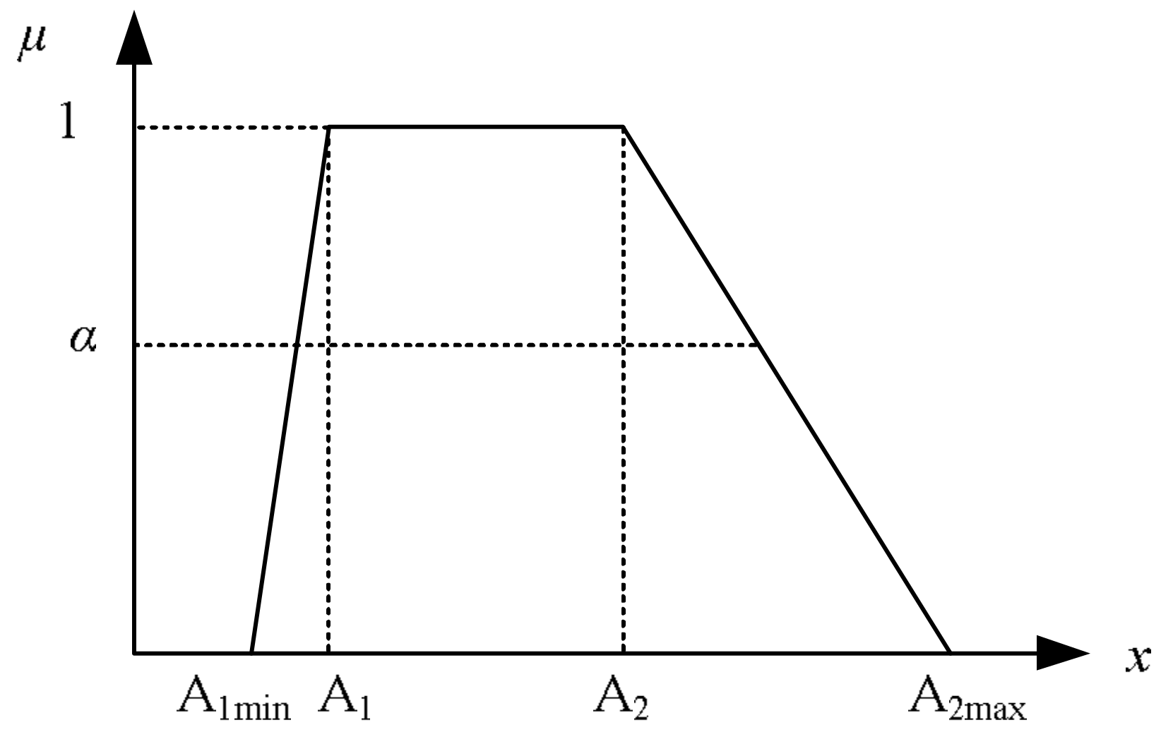
Figure 1. Trapezoid membership function.
Water 10 00488 g001
Figure 2. The schematic diagram of Equation (7).
Water 10 00488 g002
Figure 3. The schematic diagram of Equation (11).
Water 10 00488 g003
Figure 4. The schematic diagram of Equation (12).
Water 10 00488 g004
Figure 5. The study area.
Water 10 00488 g005
Figure 6. The schematic diagram of the developed FMDBLFP model.
Water 10 00488 g006
Figure 7. The upper, lower bound of yield under different α-cut levels.
Water 10 00488 g007
Figure 8. The upper, lower bound of net benefit under different α-cut levels.
Water 10 00488 g008
Figure 9. Yields of the upper-level decision-maker (ULDM), fuzzy max–min decision bi-level programming (FMDBLFP) model, and lower-level decision-maker (LLDM) under different α - cut levels.
Water 10 00488 g009
Table 1. The basic parameter of the developed model.
RegionMAi (104 mŭ)Bi (t/ mŭ)Ii (m3)EPi (104 P)LFi (t/p)Oi (yuan/m3)Si (yuan/m3)Ti (yuan/m3)WDi (104 m3)WEi (104 m3)
Liangzhou167.120.41465101.430.35.0668.86664.506303.409288.40
Minqin72.650.4545624.160.34.84131.75689.531869.304357.50
Gulang91.160.4642538.950.34.8297.21686.071145.301603.20
Tianzhu33.220.4247517.620.35.04111.05710.481196.20295.70
Table 2. The maximum and minimum water supply of planting industry, the secondary industry and the tertiary industry.
Region DistrictsPlanting Industry (104 m3)Secondary Industry (104 m3)Tertiary Industry (104 m3)
AWiminAWimaxSWiminSWimaxTWiminTWimax
Liangzhou31,393.8273,958.2010,95116,425.509211555.57
Minqin6845.3333,128.409071360.50172290.51
Gulang9449.6138,743.0012531879.50122206.06
Tianzhu5348.9315,779.5014482172.00124209.44
Table 3. The optimized irrigation areas of different irrigation districts under different α - cut levels.
Region DistrictsAi (104 mŭ)
α = 0 α = 0.2 α = 0.4 α = 0.6 α = 0.8 α = 1
Liangzhou[105.75, 159.05][108.55, 154.14][111.34, 149.41][114.14, 144.46][116.93, 139.73][119.73, 134.78]
Minqin[60.65, 60.65][60.65, 60.65][60.65, 60.65][60.65, 60.65][60.65, 60.65][60.65, 60.65]
Gulang[35.77, 35.77][35.77, 35.77][35.77, 35.77][35.77, 35.77][35.77, 35.77][35.77, 35.77]
Tianzhu[26.75, 26.55][26.75, 26.55][26.75, 26.55][26.75, 26.55][26.75, 26.55][26.75, 26.55]
Table 4. The optimization allocation of water resources for SWi and TWi under different α - cut levels.
Region Districts α   from   0   to   1
SWi (104 m3)TWi (104 m3)
Liangzhou16426.501555.57
Minqin1360.50290.51
Gulang1879.50206.06
Tianzhu2172.00209.44
Table 5. Benefits of ULDM, FMDBLFP, and LLDM under different α - cut levels.
α-Cut LevelsUBUB (108 yuan)UBLB (108 yuan)FBUB (108 yuan)FBLB (108 yuan)LBUB (108 yuan)LBLB (108 yuan)
α = 0390.45378.39390.38377.83273.85261.33
α = 0.2389.34379.05389.22378.49272.69261.98
α = 0.4388.27379.70388.11379.15271.58262.64
α = 0.6387.16380.34386.94379.81270.41263.29
α = 0.8386.10380.97385.83380.47269.30263.95
α = 1384.98381.60384.67381.12268.14264.60
Notes: UBUB, UBLB: The upper, lower bound benefit of ULDM; FBUB, FBLB: The upper, lower bound benefit of FMDBLFP; LBUB, LBLB: The upper, lower bound benefit of FMDBLFP.