Comparison of Algorithms for the Optimal Location of Control Valves for Leakage Reduction in WDNs


Abstract
:1. Introduction
2. Materials and Methods
2.1. Fitness Evaluation of the Generic Location of Control Valves
2.2. Optimal Location through Sequential Addition of Valves (SA)
2.3. Optimal Location through Multi-Objective Genetic Algorithm (GA)
3. Application
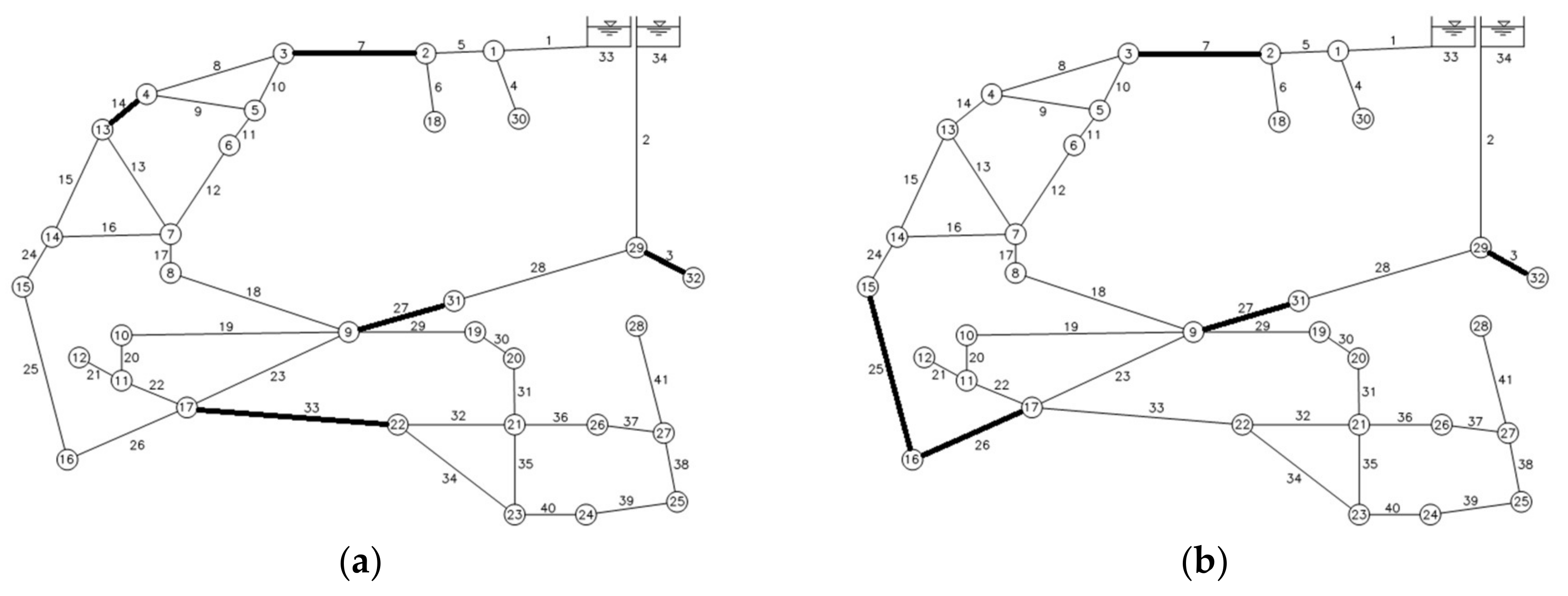
3.1. Case Studies
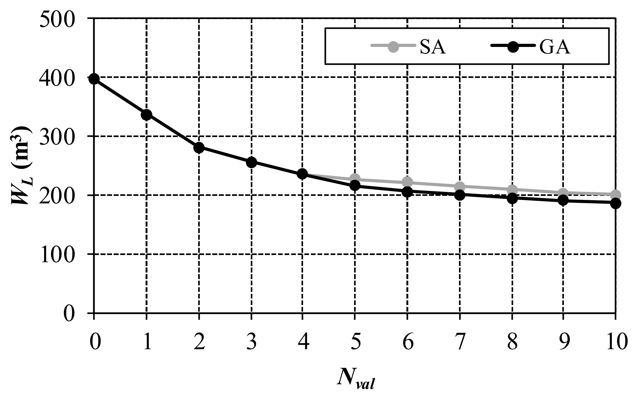
3.2. Results
4. Conclusions
Acknowledgments
Author Contributions
Conflicts of Interest
References
- Farley, M.; Trow, S. Losses in Water Distribution Networks; IWA: London, UK, 2003. [Google Scholar]
- Puust, R.; Kapelan, Z.; Savic, D.A.; Koppel, T. A review of methods for leakage management in pipe networks. Urban Water J. 2010, 7, 25–45. [Google Scholar] [CrossRef]
- Vicente, D.; Garrote, L.; Sánchez, R.; Santillán, D. Pressure Management in Water Distribution Systems: Current Status, Proposals, and Future Trends. J. Water Resour. Plan. Manag. 2016, 142, 04015061. [Google Scholar] [CrossRef]
- Sinagra, M.; Sammartano, V.; Morreale, G.; Tucciarelli, T. A new device for pressure control and energy recovery in water distribution networks. Water 2017, 9, 309. [Google Scholar] [CrossRef]
- Carravetta, A.; Del Giudice, G.; Fecarotta, O.; Ramos, H.M. Energy Production in Water Distribution Networks: A PAT Design Strategy. Water Resour. Manag. 2012, 26, 3947–3959. [Google Scholar] [CrossRef]
- Jowitt, P.W.; Xu, C. Optimal Valve Control in Water-Distribution Networks. J. Water Resour. Plan. Manag. 1990, 116, 455–472. [Google Scholar] [CrossRef]
- Campisano, A.; Creaco, E.; Modica, C. RTC of valves for leakage reduction in water supply networks. J. Water Resour. Plan. Manag. 2010, 136, 138–141. [Google Scholar] [CrossRef]
- Vairavamoorthy, K.; Lumbers, J. Leakage reduction in water distribution systems: Optimal valve control. J. Hydraul. Eng. 1998, 124, 1146–1154. [Google Scholar] [CrossRef]
- Reis, L.; Porto, R.; Chaudhry, F. Optimal location of control valves in pipe networks by genetic algorithm. J. Water Resour. Plan. Manag. 1997, 123, 317–326. [Google Scholar] [CrossRef]
- Araujo, L.; Ramos, H.; Coelho, S. Pressure control for leakage minimisation in water distribution systems management. Water Resour. Manag. 2006, 20, 133–149. [Google Scholar] [CrossRef]
- Liberatore, S.; Sechi, G.M. Location and Calibration of Valves in Water Distribution Networks Using a Scatter-Search Meta-heuristic Approach. Water Resour. Manag. 2009, 23, 1479–1495. [Google Scholar] [CrossRef]
- Ali, M.E. Knowledge-Based Optimization Model for Control Valve Locations in Water Distribution Networks. J. Water Resour. Plan. Manag. 2015, 141, 04014048. [Google Scholar] [CrossRef]
- Covelli, C.; Cozzolino, L.; Cimorrelli, L.; Della Morte, R.; Pianese, D. Optimal Location and Setting of PRVs in WDS for Leakage Minimization. Water Resour. Manag. 2016, 30, 1803–1817. [Google Scholar] [CrossRef]
- De Paola, F.; Galdiero, E.; Giugni, M. Location and Setting of Valves in Water Distribution Networks Using a Harmony Search Approach. J. Water Resour. Plan. Manag. 2017, 143, 04017015. [Google Scholar] [CrossRef]
- Pezzinga, G.; Gueli, R. Discussion of “Optimal Location of Control Valves in Pipe Networks by Genetic Algorithm.”. J. Water Resour. Plan. Manag. 1999, 125, 65–67. [Google Scholar] [CrossRef]
- Nicolini, M.; Zovatto, L. Optimal Location and Control of Pressure Reducing Valves in Water Networks. J. Water Resour. Plan. Manag. 2009, 135, 178–187. [Google Scholar] [CrossRef]
- Creaco, E.; Pezzinga, G. Multi-objective optimization of pipe replacements and control valve installations for leakage attenuation in water distribution networks. J. Water Resour. Plan. Manag. 2015, 141, 04014059. [Google Scholar] [CrossRef]
- Creaco, E.; Pezzinga, G. Embedding Linear Programming in Multi Objective Genetic Algorithms for Reducing the Size of the Search Space with Application to Leakage Minimization in Water Distribution Networks. Environ. Model. Softw. 2015, 69, 308–318. [Google Scholar] [CrossRef]
- Creaco, E.; Alvisi, S.; Franchini, M. Multi-step approach for optimizing design and operation of the C-Town pipe network model. J. Water Resour. Plan. Manag. 2016, 142, C4015005. [Google Scholar] [CrossRef]
- Giustolisi, O.; Berardi, L.; Laucelli, D.; Savic, D.; Walski, T. Battle of background leakage assessment for Water Networks (BBLAWN) at WDSA conference 2014. Procedia Eng. 2014, 89, 4–12. [Google Scholar] [CrossRef]
- Creaco, E.; Franchini, M. Comparison of Newton-Raphson Global and Loop Algorithms for Water Distribution Network Resolution. J. Hydraul. Eng. 2014, 140, 313–321. [Google Scholar] [CrossRef]
- Deb, K.; Pratap, A.; Agarwal, S.; Meyarivan, T. A fast and elitist multiobjective genetic algorithm NSGA-II. IEEE Trans. Evolut. Comput. 2002, 6, 182–197. [Google Scholar] [CrossRef]
- Carvalho, A.G.; Araujo, A.F.R. Improving NSGA-II with an adaptive mutation operator. In Proceedings of the 11th Annual Conference Companion on Genetic and Evolutionary Computation Conference: Late Breaking Papers, Montreal, QC, Canada, 8–12 July 2009; ACM: New York, NY, USA, 2009; pp. 2697–2700. [Google Scholar]
- Pezzinga, G. Procedure per la riduzione delle perdite mediante il controllo delle pressioni. In Ricerca e Controllo Delle Perdite Nelle Reti di Condotte. Manuale Per una Moderna Gestione Degli Acquedotti; Brunone, B., Ferrante, M., Meniconi, S., Eds.; CittàStudiEdizioni: Novara, Italy, 2008. (In Italian) [Google Scholar]
- Creaco, E.; Franchini, M.; Alvisi, S. Evaluating water demand shortfalls in segment analysis. Water Resour. Manag. 2012, 26, 2301–2321. [Google Scholar] [CrossRef]


| Node | z (m) | d (m3/s) | hdes (m) | Node | z (m) | d (m3/s) | hdes (m) |
|---|---|---|---|---|---|---|---|
| 1 | 465 | 0 | 14.5 | 17 | 437.6 | 0.0007516 | 15 |
| 2 | 462 | 0 | 15 | 18 | 450 | 0.0006938 | 15 |
| 3 | 456 | 0.0001156 | 15 | 19 | 442 | 0.0011563 | 15 |
| 4 | 451.3 | 0.0001156 | 15 | 20 | 436.5 | 0.00075164 | 15 |
| 5 | 451 | 0.0002891 | 15 | 21 | 433.5 | 0.0008094 | 15 |
| 6 | 448.5 | 0.0002891 | 15 | 22 | 434 | 0.0008672 | 15 |
| 7 | 444 | 0.0006359 | 15 | 23 | 431.2 | 0.000925 | 15 |
| 8 | 446 | 0.0005781 | 15 | 24 | 436.8 | 0.0008672 | 15 |
| 9 | 445 | 0.0008672 | 15 | 25 | 435.8 | 0.0008672 | 15 |
| 10 | 442 | 0.0006938 | 15 | 26 | 438.6 | 0.0006938 | 15 |
| 11 | 438.6 | 0.0006359 | 15 | 27 | 440.3 | 0.0007516 | 15 |
| 12 | 437.5 | 0.0006938 | 15 | 28 | 430.1 | 0.0008672 | 15 |
| 13 | 448 | 0.0004047 | 15 | 29 | 465 | 0.0001734 | 11 |
| 14 | 435 | 0.0004625 | 15 | 30 | 445 | 0.0003469 | 15 |
| 15 | 441 | 0.0006938 | 15 | 31 | 454 | 0.0006938 | 15 |
| 16 | 394.8 | 0.0005781 | 15 | 32 | 435 | 0.0002313 | 15 |
| Pipe | L (m) | D (mm) | k (m1/3/s) | Pipe | L (m) | D (mm) | k (m1/3/s) |
|---|---|---|---|---|---|---|---|
| 1 | 352 | 250 | 75 | 22 | 110 | 125 | 65 |
| 2 | 314 | 175 | 65 | 23 | 214 | 150 | 65 |
| 3 | 1100 | 125 | 75 | 24 | 85 | 100 | 65 |
| 4 | 350 | 100 | 65 | 25 | 398 | 100 | 65 |
| 5 | 96 | 250 | 75 | 26 | 242 | 100 | 65 |
| 6 | 282 | 100 | 75 | 27 | 118 | 175 | 65 |
| 7 | 148 | 250 | 75 | 28 | 324 | 175 | 65 |
| 8 | 256 | 250 | 75 | 29 | 140 | 125 | 65 |
| 9 | 192 | 100 | 75 | 30 | 206 | 125 | 65 |
| 10 | 58 | 100 | 75 | 31 | 70 | 125 | 65 |
| 11 | 66 | 100 | 75 | 32 | 142 | 150 | 65 |
| 12 | 230 | 150 | 75 | 33 | 86 | 150 | 65 |
| 13 | 200 | 100 | 75 | 34 | 294 | 80 | 65 |
| 14 | 44 | 250 | 75 | 35 | 150 | 80 | 65 |
| 15 | 226 | 250 | 75 | 36 | 124 | 125 | 65 |
| 16 | 70 | 150 | 65 | 37 | 144 | 125 | 65 |
| 17 | 88 | 80 | 65 | 38 | 158 | 125 | 65 |
| 18 | 204 | 125 | 65 | 39 | 130 | 80 | 65 |
| 19 | 172 | 125 | 65 | 40 | 124 | 80 | 65 |
| 20 | 94 | 125 | 65 | 41 | 500 | 80 | 65 |
| 21 | 90 | 125 | 65 |
| Time Slot (h) | Source 33–34 Head (m) | Ch (-) | Time Slot (h) | Source 33–34 Head (m) | Ch (-) |
|---|---|---|---|---|---|
| 0–2 | 480.77 | 0.40 | 12–14 | 480.55 | 1.8 |
| 2–4 | 481.14 | 0.40 | 14–16 | 480.45 | 0.90 |
| 4–6 | 481.46 | 0.55 | 16–18 | 480.64 | 0.70 |
| 6–8 | 481.22 | 1.70 | 18–20 | 480.53 | 1.45 |
| 8–10 | 480.91 | 1.25 | 20–22 | 480.19 | 1.40 |
| 10–12 | 480.94 | 1.0 | 22–24 | 480.41 | 0.45 |
| Nval | Valve Locations with SA | WL with SA (m3) | Valve Locations with GA | WL with GA (m3) | Benefits of GA (%) |
|---|---|---|---|---|---|
| 0 | - | 1243 | - | 1243 | 0.00 |
| 1 | 27 | 1029 | 27 | 1029 | 0.00 |
| 2 | 27,7 | 885 | 7,27 | 885 | 0.00 |
| 3 | 27,7,3 | 805 | 3,7,27 | 805 | 0.00 |
| 4 | 27,7,3,14 | 751 | 3,7,14,27 | 751 | 0.00 |
| 5 | 27,7,3,14,33 | 725 | 3,7,25,26,27 | 693 | 4.36 |
| 6 | 27,7,3,14,33,4 | 708 | 3,7,8,25,26,27 | 672 | 5.02 |
| 7 | 27,7,3,14,33,4,2 | 692 | 3,7,8,23,25,26,27 | 647 | 6.38 |
| 8 | 27,7,3,14,33,4,2,41 | 680 | 3,4,7,8,23,25,26,27 | 630 | 7.38 |
| 9 | 27,7,3,14,33,4,2,41,6 | 670 | 3,4,7,8,24,25,26,27,33 | 614 | 8.36 |
| 10 | 27,7,3,14,33,4,2,41,6,30 | 659 | 2,3,4,7,8,24,25,26,27,33 | 598 | 9.29 |
| Nval | Valve Locations with SA | WL with SA (m3) | Valve Locations with GA | WL with GA (m3) | Benefits of GA (%) |
|---|---|---|---|---|---|
| 0 | - | 398 | - | 398 | 0.00 |
| 1 | 27 | 338 | 27 | 338 | 0.00 |
| 2 | 27-7 | 282 | 7-27 | 282 | 0.00 |
| 3 | 27-7-3 | 257 | 3-7-27 | 257 | 0.00 |
| 4 | 27-7-3-24 | 235 | 3-7-24-27 | 235 | 0.00 |
| 5 | 27-7-3-24-8 | 228 | 3-7-25-26-27 | 217 | 4.97 |
| 6 | 27-7-3-24-8-23 | 221 | 3-8-10-25-26-27 | 206 | 6.73 |
| 7 | 27-7-3-24-8-23-20 | 215 | 3-8-10-23-25-26-27 | 201 | 6.33 |
| 8 | 27-7-3-24-8-23-20-2 | 209 | 3-4-8-10-23-25-26-27 | 196 | 6.47 |
| 9 | 27-7-3-24-8-23-20-2-4 | 204 | 3-4-8-10-20-23-25-26-27 | 191 | 6.54 |
| 10 | 27-7-3-24-8-23-20-2-4-41 | 200 | 3-4-8-10-20-23-24-25-26-27 | 187 | 6.68 |
| Nval | Valve Locations with SA | WL with SA (m3) | Valve Locations with GA | WL with GA (m3) | Benefits of GA (%) |
|---|---|---|---|---|---|
| 0 | - | 119 | - | 119 | 0.00 |
| 1 | 49 | 114 | 49 | 114 | 0.00 |
| 2 | 49-45 | 113 | 15-45 | 112 | 1.14 |
| 3 | 49-45-15 | 107 | 15-25-45 | 107 | 0.00 |
| 4 | 49-45-15-5 | 103 | 5 -15-45-49 | 103 | 0.00 |
| 5 | 49-45-15-5-27 | 102 | 7-15-38-45-49 | 100 | 1.85 |
| 6 | 49-45-15-5-27-7 | 101 | 5 -7-15-25-38-45 | 96 | 4.32 |
| 7 | 49-45-15-5-27-7-38 | 95 | 5-7-25-32-38-39-45 | 95 | 0.09 |
| 8 | 49-45-15-5-27-7-38-52 | 94 | 5-7-15-32-38-39-45-49 | 92 | 2.61 |
| 9 | 49-45-15-5-27-7-38-52-33 | 94 | 5-7-15-25-27-32-38-39-45 | 90 | 3.92 |
| 10 | 49-45-15-5-27-7-38-52-33-30 | 93 | 5-7-15-27-32-33-38-39-45-49 | 89 | 4.05 |
© 2018 by the authors. Licensee MDPI, Basel, Switzerland. This article is an open access article distributed under the terms and conditions of the Creative Commons Attribution (CC BY) license (http://creativecommons.org/licenses/by/4.0/).
Share and Cite
Creaco, E.; Pezzinga, G. Comparison of Algorithms for the Optimal Location of Control Valves for Leakage Reduction in WDNs. Water 2018, 10, 466. https://doi.org/10.3390/w10040466
Creaco E, Pezzinga G. Comparison of Algorithms for the Optimal Location of Control Valves for Leakage Reduction in WDNs. Water. 2018; 10(4):466. https://doi.org/10.3390/w10040466
Chicago/Turabian StyleCreaco, Enrico, and Giuseppe Pezzinga. 2018. "Comparison of Algorithms for the Optimal Location of Control Valves for Leakage Reduction in WDNs" Water 10, no. 4: 466. https://doi.org/10.3390/w10040466
APA StyleCreaco, E., & Pezzinga, G. (2018). Comparison of Algorithms for the Optimal Location of Control Valves for Leakage Reduction in WDNs. Water, 10(4), 466. https://doi.org/10.3390/w10040466