Stochastic Linear Programming for Reservoir Operation with Constraints on Reliability and Vulnerability

Abstract

Reliability and vulnerability (RV) are two very important performance measures but, due to their stage-inseparable nature, they cannot be explicitly incorporated in stochastic dynamic programming (SDP), which is extensively used in reservoir operation. With inflows described as a Markov chain, a stochastic linear programming (SLP) model is formulated in this paper to explicitly incorporate the RV constraints in the reservoir operation, aimed at maximizing the expected power generation by determining the optimal scheduling decisions and their probabilities. Simulation results of the SLP and SDP models indicate the equivalence of the proposed SLP and SDP models without considering the RV constraints, as well as the strength of the SLP in explicitly incorporating the RV constraints. A simulated scheduling solution also reveals a reduction of power generation fluctuation, with the reservoir capacity emptied in advance to meet given reliability and vulnerability.

1. Introduction

Generally being “high-dimensional, dynamic, nonlinear, and stochastic” [1], a water resource system is difficult to optimize. To solve such a complex problem, many researchers have attempted a variety of methods, mainly focused on models and algorithms, which are complementary in different situations. As the most mature mathematical programming, linear programming (LP) and dynamic programming (DP) provide two different ways of solving water resource planning problems. LP is one of the most widely used mathematical programming methods owing to its strict mathematic theory and general solution in hydropower management. Generally, a standard form is required for an LP model to be solved by an efficient generic solver. Based upon Bellman’s optimality principle, DP is only applicable to stage-separable processes and encounters difficulties of so-called “curse of dimensionality” for exponential growth of variables in the growth of dimensionality.

Since randomness always accompanies the application of LP and DP, the stochastic characteristics generally cannot be ignored. Moreover, the handling of random characteristics has a profound influence on optimization or simulation performance. According to different treatments of stochastic characteristics, the deterministic and stochastic models represent two patterns. The deterministic model regards the stochastic hydrologic parameters as known quantities. This treatment reduces the complexity of the model to some extent. Nevertheless, the simplification cannot retain all the essential characteristics of the original data, and may lead to unsatisfactory results. Integrating the stochastic information represented in different ways into an LP or DP model, a variety of stochastic models has been developed.

With the randomness involved, stochastic dynamic programming (SDP) has been so extensively used in reservoir operation, and its selection of state and decision variables has brought different models. Among them, Bras et al. [2] incorporated current hydrologic forecast information in an SDP model. Stedinger et al. [3] incorporated available hydrologic information into an SDP decision model by using the streamflow forecast as the hydrologic state variable. Kelman et al. [4] introduced sampling stochastic dynamic programming (SSDP) to optimize water system operations on the Feather River in California (USA) using multiple historical streamflow time series as scenarios to capture the variability of streamflow processes by example. Another method to incorporate stochastic information into SDP is Bayesian SDP. Karamouz and Vasiliadis [5] described streamflow with a discrete lag 1 Markov process and updated the probabilities with new information; it showed that the forecast of the next period’s flow as state variables performed better than that used for the forecast of the current period’s flow. Xu et al. [6] proposed a new two-stage Bayesian stochastic dynamic programming model which partitions the forecast horizon into two periods.

The SDP requires an objective and constraints to be stage-separable, which prevents it from explicitly incorporating many performance criteria into its formulation. Chen [7] developed a fuzzy dynamic programming approach by applying the fuzzy iteration model to evaluate the decisions at each stage. In many cases, however, these criteria of a system are the most critical aspects that should be considered. The fundamental performance indices include the mean, variance, and deficit of statistical values. For example, the mean, variance of statistical power generations is used to evaluate the performance of a hydropower station. Other evaluation indices have also been put forward, including the robustness by Hashimoto et al. [8] and sustainability in a water resource system by Loucks [9] and Sandoval-Solis [10]. Hashimoto et al., in 1982 [11], introduced systematically three criteria: the reliability (how likely the system is to fail), vulnerability (how severe the consequences of failure may be), and resilience (how quickly a system recovers from failure), abbreviated as RRV criteria.

The RRV criteria were the most widely used in different water resource systems. Moy et al. [12] optimized these three measures and revealed relationships among them regarding a water supply reservoir using multi-objective mixed-integer linear programming. Kundzewicz et al. [13] found that conflicts between particular criteria might arise. In the literature of Zhang et al. [14], both conflicting and synergetic relationships were found between reliability, vulnerability and resilience using many-objective analysis. Based on the assumption of stationary hydrology, a joint analysis of multi-criteria was carried out by Jain and Bhunya [15], in which the behavior of statistical performance indices, namely the RRV, of a multipurpose storage reservoir was examined. They used a probabilistic approach to interpret the behavior of these indices and computed several performance indices for each sequence simulated by the Monte Carlo method and presented a framework for a multi-criteria approach that computed all the relevant quantities for each time period in reservoir design and management. The statistical behaviors of three indices were examined using input data by the Monte Carlo method. Some researchers combined these three performances to evaluate the performance of water resources systems. Loucks [9] combined RRV into an index to quantify sustainability. After that, the sustainability index (SI) was utilized in Kay’s research [16] to help identify decisions. New combinations of RRV, such as, a combined reliability–vulnerability index and a robustness index were utilized via fuzzy set theory by Ibrahim El-Baroudy et al. [17]. The RRV or sustainability index tend to be applied in the field of climate change on water resources systems [18,19].

The possibility of explicitly incorporating the RRV constraints into a stochastic linear programming (SLP) has not been investigated in previous works, especially hydropower system operation. Applications of the SLP in reservoir operation are not new, though only a small amount of literature is available on the pure application of the SLP. Among the scarce previous literature, Loucks [20] presented an SLP model, where the random and serially correlated inflows were described with a first-order Markov chain. Lee et al. [21] developed a two-stage SLP model based on the form of a “fan of individual scenarios” to coordinate the multi-reservoir operation. Using inflow scenarios generated by a multivariate periodic AR(1) model considering serial and spatial connections, a stochastic model indicates its advantages over a deterministic model and its effectiveness in real-time operation. Baliarsingh and Kumar [22] developed a form of stochastic linear programming in which the decision variables were the joint probabilities of the reservoir release given an initial reservoir storage volume, an inflow, and the final storage volume for a given time period. System performance was set as the sum of squared deviations from target storage and target release.

In view of the lack of an SLP model which takes the reliability and vulnerability criteria into consideration, this paper will explore the possibility to incorporate the constraints on reliability and vulnerability (RV) into an SLP model to maximize the expected power generation in reservoir operation. The model will introduce a new variable, namely, the probability of reservoir capacity at the end of the time period when reservoir capacity at the beginning of the time period and inflow during the time period have been given. The inflows will be described as a Markov chain because of their uncertainty. The IBM CPLEX software (IBM, Armonk, NK, USA), a convenient and excellent LP solver, will be employed to solve the SLP model, which is expected to have numerous combinations of discrete representative values. Since both the SLP and SDP can handle the reservoir operation problem when the RV constraints are not involved, their results will be compared to illustrate their equivalence in this situation. This work will also investigate the capability of the SLP to explicitly incorporate the RV constraints, showing its advantage over the SDP.

2. Problem Formulation

The problem is formulated to determine a closed-loop feedback operational policy that maximizes the expected energy production while meeting the power yield with required minimum reliability and maximum vulnerability. The inflows are described as a Markov chain and represented with representative values and transition probability matrices. The conditional probabilities of final reservoir volumes, given the initial volumes and representative inflows for each time period, as a variable to be solved, are introduced. Simultaneously, a binary variable whose value can only be taken as 0 or 1, representing whether the decision is made or not, is set as another variable to be solved.

2.1. Objective

Mathematically, the objective is to maximize the expected generation, expressed as

$$\max {\displaystyle \sum _{t=1}^T{\displaystyle \sum _{(i,k,l)\in \Omega (t)}(P_{iklt}\cdot G_{iklt}\cdot \Delta t)}}$$

(1)

where $T$ is the number of the time period; $t$ is the time period index; $\Delta t$ is the time length in hours of time period $t$; $i$ is the index representing the discretization values of storage at the beginning of time period $t$; $k$ is the index representing the characteristic values of inflow during time period $t$; $l$ is the index representing the discretization values of storage at the end of time period $t$, and also the index representing the value of storage at the beginning of time period $t+1$; $P_{iklt}$ is the probability of being at state $(i,k)$ and making the decision $(l)$ at the beginning of $t$, expressed as $l=\ell \left(i,k,t\right)$, which stands for the target storage at the end of time period $t$ and is determined by the inflow $k$ in $t$ and storage $i$ at the beginning of $t$; $\Omega (t)$ is the feasible combinations of state and decision variables; and $G_{iklt}$ is the power generation in GW produced in time period $t$,

$$G_{iklt}=G\left[S_t^{(i)},Q_t^{(k)},S_{t+1}^{(l)}\right]$$

(2)

which is calculated with the approximate formula proposed in Wang’s paper [23],

$$G_{iklt}=G\left[S_t^{(i)},Q_t^{(k)},S_{t+1}^{(l)}\right]=\eta \cdot \left[h^{\min }+\alpha \sqrt{0.5(S_t^{(i)}+S_{t+1}^{(l)})}\right]\cdot \min \left[R_t(i,k,l),U^{\max }\right]$$

(3)

Here, $\eta$ is the energy conversion factor used to convert m⁴/s into $\mathrm{GW}$; $h^{\min }$ is the minimal water head in m; $\alpha$ is a coefficient associated with the reservoir shape, which in this paper is determined by solving

$$h_i^{\max }=h_i^{\min }+\alpha \cdot \sqrt[3]{S_i^{\max }}$$

(4)

$S_t^{(i)}$ is the $i\text{th}$ characteristic storage value in m³ at the beginning of $t$; $S_{t+1}^{(l)}$ is the $j\text{th}$ characteristic storage value in m³ at the end of $t$, also the characteristic storage value in m³ at the beginning of $t+1$; $Q_t^{(k)}$ is the $k\text{th}$ characteristic inflow value in m³/s in $t$; $U^{\max }$ is the outflow capacity in m³/s for generation; and $R_t(i,k,l)$ is the release in m³/s in time period $t$, determined by

$$R_t(i,k,l)=\frac{1}{\Delta t}\left[S_t^{(i)}-S_{t+1}^{(l)}\right]+Q_t^{(k)}$$

(5)

2.2. General Constraints

The constraints include the following:

(1) The joint probabilities for any time period must sum to 1.0,

$${\displaystyle \sum _{(i,k,l)\in \Omega (t)}{P}_{iklt}}=1(\forall t)$$

(6)

which means that the decision in time period $t$ must be one of the feasible decisions.

(2) The probability transition satisfies

$${\displaystyle \sum _{(i,k)\in \Omega (t)}{P}_{iklt}\cdot P_{kj}^{[t]}}={\displaystyle \sum _{m\in \Omega (t+1)}{P}_{l,j,m,t+1}}for(l,j)\in \Omega (t+1)$$

(7)

where $P_{kj}^{[t]}$ is the transition probability, defined as the probability that the $j\text{th}$ characteristic inflow in time period $t+1$ occurs given that the $k\text{th}$ inflow has been observed in time period $t$. This constraint implies that any state in the next time period $t+1$ is ruled by the decision and by the transition probabilities in the current time period $t$.

(3) Decision uniqueness should be enforced on

$${\displaystyle \sum _{l\in \Omega (t)}{u}_{iklt}=1}for\left(i,k\right)\in \Omega (t)$$

(8)

and

$$P_{iklt}\le u_{iklt}for\forall (i,k,l)\in \Omega (t)$$

(9)

where $u_{iklt}$ is a binary variable that decides whether or not decision $l$ is made at state $(i,k)$ in time period $t$, which implies that only one of the optional target storage values at the end of a time period must be selected given the state at the beginning of the time period.

2.3. Reliability and Vulnerability Constraints

Owing to the introduction of conditional probability variables, as well as to the expression of reliability and vulnerability corresponding to the probability of meeting requirements and expected violation, the two performances can be explicitly expressed in the SLP model.

2.3.1. Reliability

Reliability has been a primary performance metric in evaluating operational system stability. In reservoir operation, reliability is measured by the probability of a system being in a satisfactory state. In this paper, since joint probability variables have been introduced, the average value of the sum of all probabilities satisfying generation requirements is used to assess reliability performance logically. The reliability performance should be no less than a preset percentage $\beta$, expressed as

$$\frac{1}{T}{\displaystyle \sum _{t=1}^T{\displaystyle \sum _{(i,k,l)\in \Theta (t)}{P}_{iklt}}\ge \beta }$$

(10)

where $\Theta (t)$ is a subset of $\Omega (t)$ and consists of the feasible combinations $(i,k,l)$ in time period $t$ that meet the generation yield, i.e.,

$$\Theta (t)=\left\{(i,k,l)|G_{iklt}\ge Y;R_t(i,k,l)\ge 0\right\}$$

(11)

in which $Y$ is the generation yield in GW. Here, the reliability is defined as the probability that the generation yield is met.

2.3.2. Vulnerability

Reliability is without question a criterion that should not be ignored during water resources system operation. Generally speaking, higher reliability of an operational system is always desired. However, from the reliability criterion, we can only evaluate how much the system can operate to fulfill the requirements. A failure cannot be avoided. When the failure occurs, to what extent the damage can cause an unsatisfactory situation, or what the likely magnitude of such a situation is, is always of concern. Similarly, the expected quantification of violations in all time periods is used to quantify the vulnerability performance.

The vulnerability should be less than a preset value $\nu$,

$$\frac{1}{T}{\displaystyle \sum _{t=1}^T{\displaystyle \sum _{(i,k,l)\in \overline{\Theta }(t)}{P}_{iklt}}}\left(Y-G_{iklt}\right)\le \nu$$

(12)

where $\overline{\Theta }(t)$ is the relative complementary set of $\Theta (t)$ with respect to $\Omega (t)$, $\nu$ is given before the calculation which indicates how much the average power generation yield can violate. Here, the vulnerability is defined as the expected violation of the generation yield when the violations occur.

3. Solution Procedure

Evidently, in view of the fact that the probability transition matrices for each time period can be derived, objectives and constraints in the model are linear. It can therefore be solved using an LP solver. Without considering the RV constraints, the SDP model is applied to obtain the optimal strategy compared with the SLP model.

3.1. Inflow Description and Probability Transition Matrices

The reservoir inflow is described as a periodic first-order Markov chain. State and transition probability are two critical concepts in a Markov chain for describing inflow in each particular time period. The inflow is divided into $m$ intervals for each time period, and each state is represented by an average value $Q_t^k$ for each interval. Thus, the probability transition matrices $P_{kj}^{[t]}$ that are used to describe the probabilities of a representative value $Q_{t+1}^j$ in time period $t+1$ given a representative value $Q_t^k$ in time period $t$ are derived by frequency analysis. The reservoir capacity discrete value takes on arithmetic sequences between dead reservoir volume and maximum volume.

3.2. Solving the SLP Model

With the sets $\Omega (t)$, $\Theta (t)$, and $G_{iklt}$ predetermined, as well as inflow transition probability $P_{kj}^{[t]}$ derived, the model becomes a mixed integer linear programming with objective (1) subject to (6)–(10) and (12). Owing to the existence of 0–1 binary variables $u_{iklt}$, the model is complicated to solve. However, benefiting from the standard mathematical form of linear programming and the improvement of computer performance, many efficient and convenient solvers are available, including CPLEX (IBM, Armonk, NY, USA), YALMIP (Johan Löfberg, Jekyll & Minimal Mistakes), and GUROBI (GUROBI, Houston, TX, USA), which make solving large-scale optimization problems with thousands of variables possible. In this work, the goal is to determine the following decision variables: the binary $u_{iklt}$ and the probabilities $P_{iklt}$.

3.3. Solving the SDP Model

Though it is very difficult, if not impossible, for the SDP to incorporate the RV constraints, the SDP is actually very powerful in dealing with stochastic sequential decision-making process problems. Here, a universal reservoir operation problem is formulated as an SDP model, where the state variables are as follows: the storage $S_t$ at the beginning of time period t and inflow $Q_t$ into a reservoir during time period t; and the decision variables are as follows: storage values $S_{t+1}$ at the end of time period t.

The recursive equation is expressed as

$$f_t\left(S_t,Q_t\right)=\underset{S_{t+1}}{\max }[G(S_t,Q_t,S_{t+1})+\underset{\langle Q_{t+1}|Q_t\rangle }{E}{f}_{t+1}\left(S_{t+1},Q_{t+1}\right)]$$

(13)

where $f_t\left(S_t,Q_t\right)$ is the maximum expected power generation corresponding to a set of $S_t$ and $Q_t$ over the remaining time periods of the time horizon; and $G(\cdot )$ is the immediate power generation in time period $t$; $\underset{\langle Q_{t+1}|Q_t\rangle }{E}$ is the conditional expectation operator over $Q_{t+1}$ given $Q_t$.

In order to obtain a stationary operation policy, a backward recursion should be implemented in several cycles, starting with $f_T\left(S_T,Q_T\right)=0$. The maximum expected benefit $f_t\left(S_t,Q_t\right)$ over the remaining time period from $t$ to $T$ is calculated for each given $S_t$ and $Q_t$. The aforementioned recursive calculation continues until a convergent and stable policy is obtained.

4. Case Studies

The stochastic dynamic programming cannot explicitly incorporate the RV constraints. The Xiaowan and Nuozhadu hydropower reservoirs in Yunnan Province, China, are used as case studies to verify the effectiveness of the stochastic linear model in obtaining an operating policy and the equivalence between the proposed SLP without RV constraints and the SDP model.

Using 56 years of one-third-monthly (at an interval about 10 days) historical inflows of Xiaowan and Nuozhadu Reservoirs during 1953–2008 and also 1490 years of one-third-monthly inflows of Xiaowan Reservoir simulated by AR(2), the representative inflows are divided into seven states, and the 7 $\times$ 7-dimensional matrices representing the transition probability are calculated based on the previously mentioned first-order Markov chain for each time period. Karamouz and Houck [24] showed that 20 storage values could be adequate for a reservoir with storage capacity of up to 170% of the mean annual flow. For convenience of calculation, a number of 21 representative discrete storage values are set evenly.

In view of its rapid solving ability and language-support features, CPLEX12.6 (IBM, Armonk, New York, USA) was employed to solve the SLP model in this work.

4.1. Comparison between the SLP and SDP Models without the RV Constraints

Without considering the RV constraints, the unknown decision variables $u_{iklt}$ and corresponding decision probabilities $P_{iklt}$ can be derived by solving the SLP model. There are two ways to calculate statistical values, one based on parameters and variables in the SLP model, and another one by operation simulation with sample inflows following an optimal decision rule derived either from the SLP or SDP results. 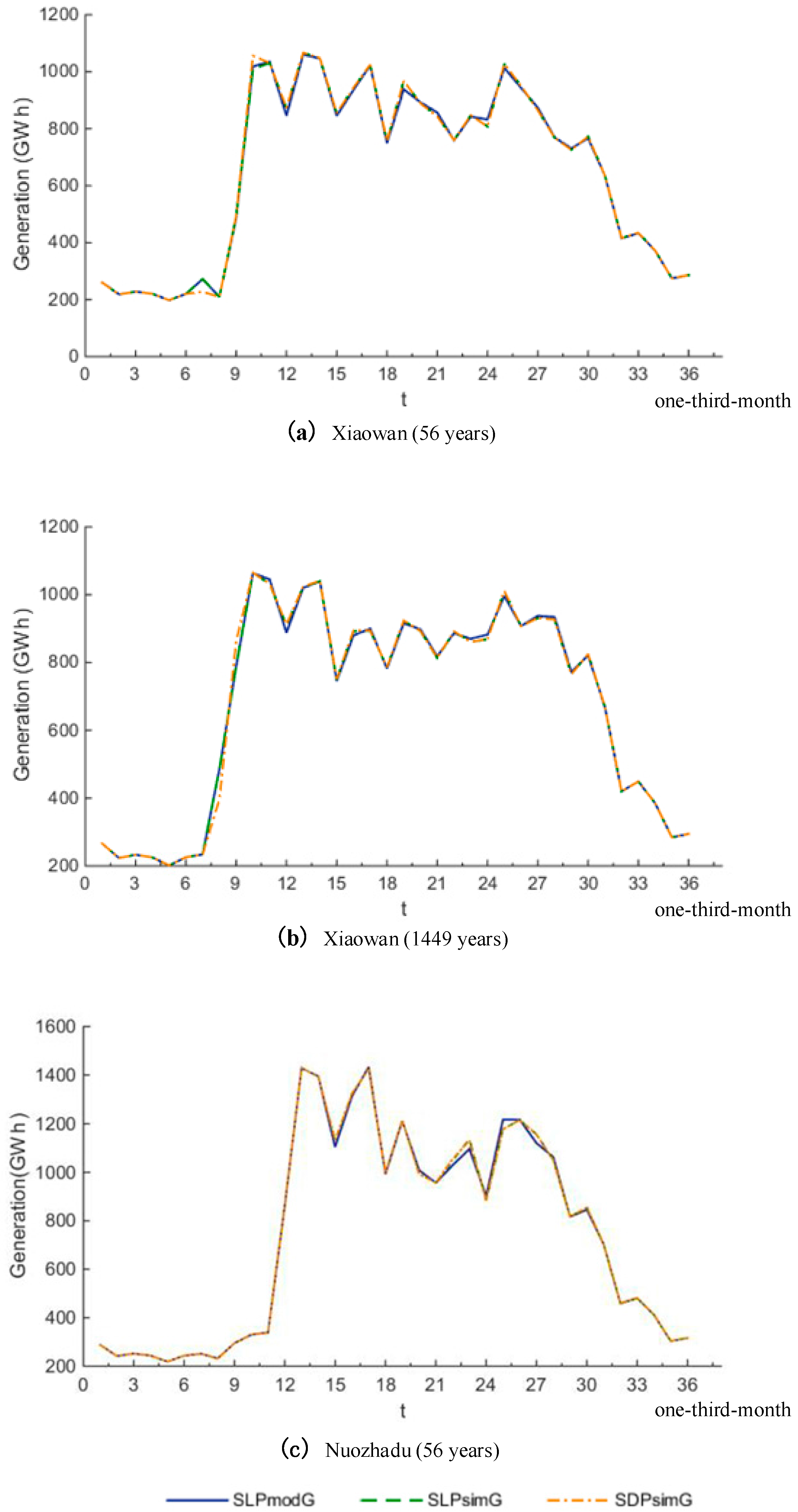Figure 1 shows the expected one-third-monthly power generations derived by the SLP model, and the statistical annual power generation trajectory obtained by simulation based on SLP and SDP decisions. The results indicate that the expected generation trajectory calculated in the SLP and the averaged generation trajectory when simulated based on the SLP and SDP solutions are almost the same. The SDP has long been proven capable of producing the optimal decision rule, which, then, can also be achieved by the SLP model.

Table 1. Annual energy production in GWh by the SLP model (SLPmod), and by simulation for the SLP (SLPsim) and SDP (SDPsim) without RV constraints.

Calculation Ways	Xiaowan His.	Xiaowan Sim.	Nuozhadu His.
SLPmod	23,504.5	24,389.7	26,619.8
SLPsim	23,568.3	24,391.4	26,684.2
SDPsim	23,568.6	24,390.5	26,684.1

gives the statistical annual energy production when adopting different sample inflows, namely 56 years of one-third-monthly inflows historically observed for Xiaowan and Nuozhadu reservoirs and 1449 years of one-third-monthly inflows simulated for the Xiaowan Reservoir. Statistical annual energy productions derived by simulating the SLP and SDP decision rules are almost identical, either for the 56 years of historical inflows or the 1449 years of simulated inflows. Simulating the decision rules, when employing the 56 years of historical inflows, gives averaged annual energy productions approximately 0.2–0.3% greater than those theoretically determined in the SLP model. The gap, however, can be reduced to within 0.007% by using the 1449 years of simulated inflows to diminish the sample errors. It is thus concluded that the SLP and SDP models without considering the reliability and vulnerability constraints can produce an identical solution to optimally operate a reservoir.

4.2. Result of the SLP Model with the RV Constraints

With 1449 years of artificially generated one-third-monthly inflows of Xiaowan reservoir, the SLP model is formulated and solved to evaluate the influence of the RV constraints on the behavior of reservoir operation.

Table 2. Comparison of model and simulated (Sim) values of expected power generation (Exp. G), reliability, and vulnerability for each time period with (Y, β, v) = (1.778, 0.98, 0.01).

Time Period	Exp. G (GWh)		Reliability		Vulnerability
	Model	Sim	Model	Sim	Model	Sim
1	565.52	565.91	1.000	0.999	0.0008	0.0005
2	521.67	521.77	1.000	0.997	0.0000	0.0007
3	528.33	528.44	1.000	0.999	0.0000	0.0006
4	518.05	518.17	1.000	0.999	0.0000	0.0006
5	492.88	493.01	1.000	0.983	0.0000	0.0012
6	513.34	513.50	1.000	0.998	0.0000	0.0006
7	518.37	518.54	1.000	0.990	0.0000	0.0009
8	531.56	525.57	0.963	0.946	0.0126	0.0242
9	549.91	550.26	1.000	0.994	0.0000	0.0006
10	575.74	576.35	0.999	0.995	0.0011	0.0006
11	578.61	579.10	0.998	0.967	0.0007	0.0040
12	607.22	609.45	0.988	0.977	0.0067	0.0098
13	547.20	543.84	0.921	0.912	0.0705	0.0702
14	570.52	572.71	0.980	0.948	0.0059	0.0085
15	616.19	623.16	0.931	0.951	0.0051	0.0082
16	643.97	644.45	1.000	0.968	0.0000	0.0059
17	673.59	667.30	0.965	0.966	0.0152	0.0100
18	767.28	774.60	1.000	0.996	0.0000	0.0006
19	746.00	745.96	1.000	0.954	0.0000	0.0170
20	825.48	814.86	0.948	0.948	0.0055	0.0220
21	809.98	806.48	1.000	0.983	0.0000	0.0046
22	851.21	855.25	1.000	0.984	0.0000	0.0066
23	864.13	858.83	0.961	0.946	0.0433	0.0343
24	857.16	847.16	1.000	0.978	0.0000	0.0087
25	888.24	890.25	1.000	0.979	0.0000	0.0083
26	902.43	901.37	0.948	0.944	0.0525	0.0306
27	890.18	889.46	0.989	0.939	0.0035	0.0230
28	906.55	915.71	0.943	0.944	0.0395	0.0349
29	865.72	856.29	0.999	0.987	0.0002	0.0013
30	802.89	808.26	0.982	0.963	0.0032	0.0071
31	674.16	670.77	0.910	0.940	0.0373	0.0497
32	583.68	586.13	0.966	0.963	0.0098	0.0056
33	555.31	553.79	0.936	0.936	0.0299	0.0325
34	591.11	600.74	0.955	0.992	0.0163	0.0037
35	588.57	588.92	1.000	1.000	0.0002	0.0000
36	596.25	596.50	1.000	0.999	0.0003	0.0007
Sum	24,118.998	24,112.841	-	-	-	-
Avg.	669.97216	669.80115	0.97999	0.97118	0.01	0.01216

presents the results detailed in each time period when parameters Y, β and v are set to 1.778, 0.98 and 0.01, respectively. Again, the expected energy production, the reliability and the vulnerability at each time period are all calculated in two ways, one by the SLP model itself, and another one through operation simulation following the optimal decision rule derived by the SLP model.

Table 2 shows that the power generation trajectory, reliability, and vulnerability in each time period, by both the model and simulation, are very close, though the gap of vulnerability is slightly larger relative to the other two indices. Similarity is also found in the cumulative power generation, averaged reliability and vulnerability over a representative year. The closeness suggests that the discretization resolution of both the storage capacity and the possible inflow is good enough for the SLP model to obtain an optimal decision rule that can achieve what the SLP model expects for many years of reservoir operation.

Changing the power generation yield $Y$, reliability $\beta$, and vulnerability $\nu$ will yield different solutions by solving the SLP model, with some feasible and some infeasible.

Table 3. Annual power generation (GWh) by the SLP model itself and by operation simulation with different parameters.

No.	Combinations ($\mathit{Y}$, $\mathit{\beta }$, $\mathit{\nu }$)	Model	Simulation
1	(1.778, 0.98, 0.01)	24,119	24,112
2	(1.778, 0.98, 0)	24,169	24,167
3	(1.778, 0, 0.01)	24,196	24,183
4	(2.5, 0.7, 0.3)	24,076	24,061
5	(2.5, 0.6, 0.3)	24,258	24,247

gives five feasible combinations of $Y$, $\beta$ and $\nu$, as well as the annual energy productions derived by the model itself and by the operation simulation following the optimal decision rule. There is a very small gap between the model and simulated results for cumulative power generation. As shown in Table 3, the model and simulated results derived with 1449 years of simulated inflows are very close to each other.

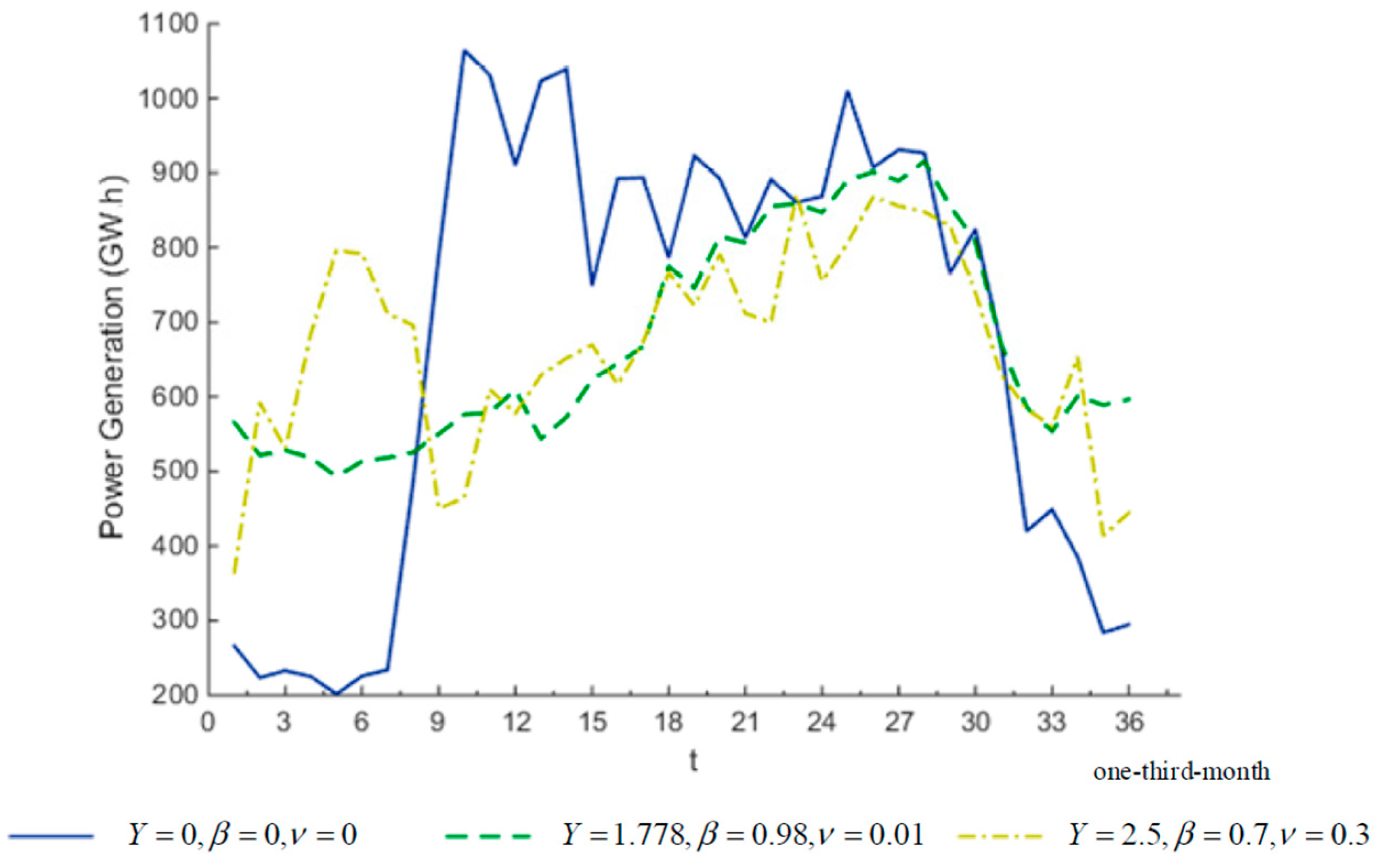
Figure 2 shows the statistical results of the power generation trajectory by 1449 years of operation simulations when the power yield $Y$, reliability $\beta$, and vulnerability $\nu$ are set to (0, 0, 0), (1.778, 0.98, 0.01), and (2.5, 0.7, 0.3), respectively. The results indicate that enforcing a power yield with certain RV constraints will achieve a more even power generation over time despite less energy production occurring. By trial and error, the power yield can be improved from 1.778 GW to 2.5 GW only to the detriment of the reliability by 28% = 98% − 70%. With the power yield and reliability set to 2.5 GW and 70% respectively, the minimum vulnerability can be achieved at 0.3. It seems that in this case study, the higher reliability also benefits a lower vulnerability.

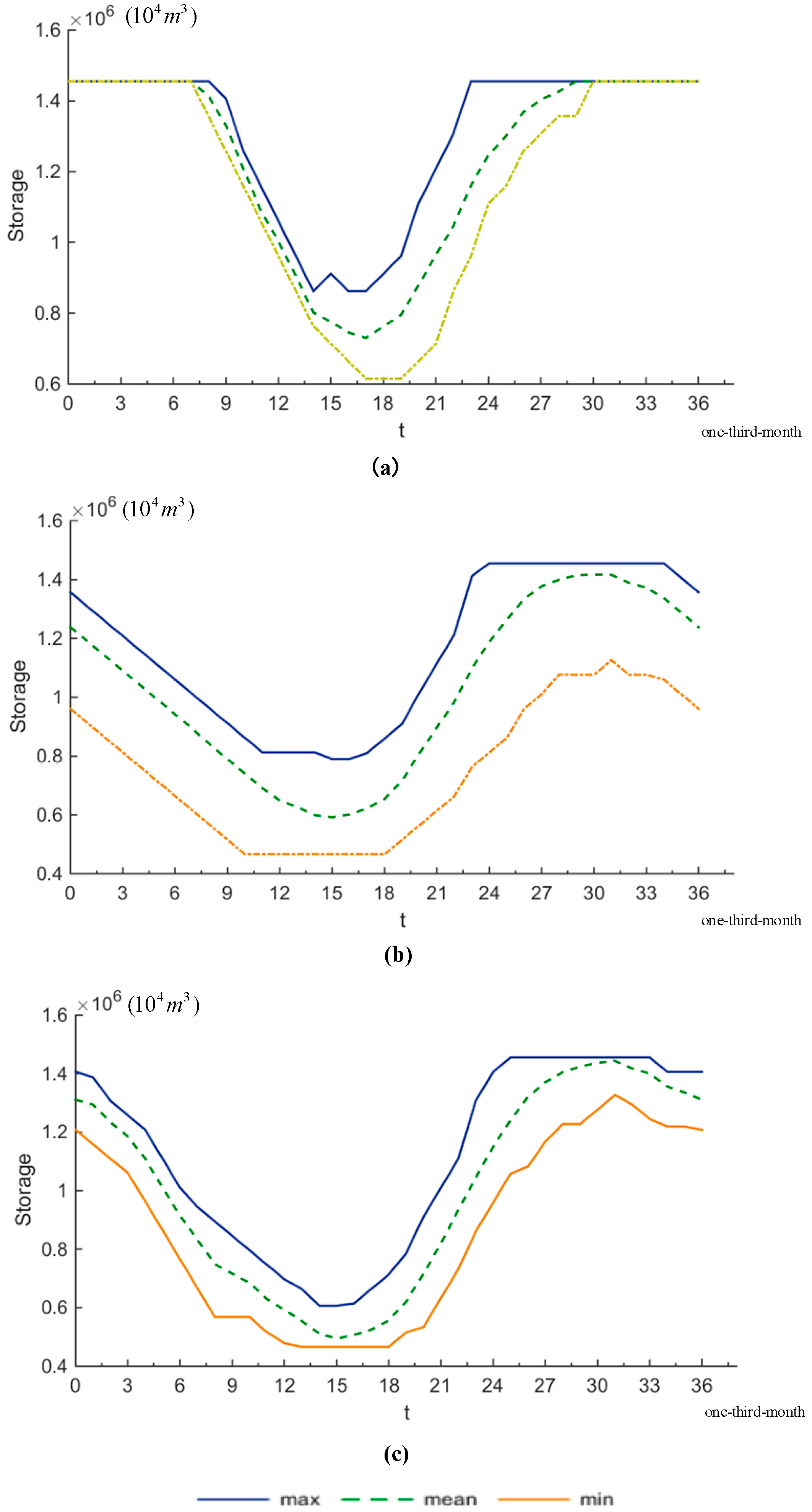
Figure 3 shows the maximum, average and minimum of one-third-monthly storages in a representative year, calculated by operation simulation with 1449 years of artificially generated inflows for combinations ($Y$, $\beta$, $\nu$) = (0, 0, 0), (1.778, 0.98, 0.01), and (2.5, 0.7, 0.3), respectively. Without enforcement on the power yield and its reliability and vulnerability for ($Y$, $\beta$, $\nu$) = (0, 0, 0), the SLP model will derive an optimal decision rule that maximizes the energy production by keeping the storage level as high as possible unless it is beneficial to empty the reservoir to alleviate spillages. With a power yield $Y$ = 1.778 GW, the reservoir is utilizing its storage during the dry seasons to achieve a high reliability $\beta$ = 98% and a low vulnerability $\nu$ = 0.01 to the detriment of energy production as a whole. Comparing (b) and (c) in Figure 3, it is interesting to find that increasing the power yield from 1.778 GW to 2.5 GW narrows the operational space of the reservoir, which operates in a smaller corridor confined by the maximum and minimum storages.

5. Conclusions

This paper presents a stochastic linear programming (SLP) model with strength over SDP in that it explicitly incorporates reliability and vulnerability (RV) constraints. The stochastic characteristics of inflow are captured by Markov transition matrices. The IBM’s CPLEX LP solver (IBM, Armonk, NK, USA) is employed to solve the SLP model, which, without enforcing the RV constraints, produces solutions equivalent to those by the SDP model, which has long been proved effectively in reservoir operation. With 1449 years of one-third-monthly inflows artificially generated by an AR(2) model, the SLP model evinces its capability to take into account the RV constraints. The case studies also show that a higher power yield can evidently result in difficulty to meet stricter reliability and vulnerability requirements. Meanwhile, adding the RV constraints decreases the power generation, but can make the power generation more reliable and less vulnerable.

The proposed SLP model can also be used to conduct a tradeoff analysis among the power yield, reliability and vulnerability. The performance resilience has a more complicated expression than the reliability and vulnerability, and its possibility to be explicitly incorporated into the SLP model needs to be investigated in future works.