Multiple Climate Change Scenarios and Runoff Response in Biliu River

Abstract

The impacts of temperature and precipitation changes on regional evaporation and runoff characteristics have been investigated for the Biliu River basin, which is located in Liaoning Province, northeast China. Multiple climate change scenarios from phase 3 and phase 5 of the Coupled Model Intercomparison Project (CMIP3 and CMIP5) (21 scenarios in total) were utilized. A calibrated hydrologic model—SWAT model—was used to simulate future discharges based on downscaled climate data through a validated morphing method. Results show that both annual temperature and precipitation increase under most of the CMIP3 and CMIP5 scenarios, and increase more in the far future (2041–2065) than in the near future (2016–2040). These changes in precipitation and temperature lead to an increase in evaporation under 19 scenarios and a decrease in runoff under two-thirds of the selected scenarios. Compared to CMIP3, CMIP5 scenarios show higher temperature and wider ranges of changes in precipitation and runoff. The results provide important information on the impacts of global climate change on water resources availability in the Biliu River basin, which is beneficial for the planning and management of water resources in this region.

1. Introduction

It has been recognized that climate change could have profound impacts on the global water cycle [1,2,3]. Therefore, it is important to consider potential impacts of climate change in the planning and management of regional water resources.

To quantitate climate change impacts on water resources, the output of general circulation models (GCMs) is commonly used [4,5,6], coupled with hydrological models or forcing offline hydrological models [7,8,9,10]. The results help to understand the impacts of climate change and develop strategies to adapt to or possibly mitigate these impacts [3]. The Coupled Model Intercomparison Project phase 3 (CMIP3) and phase 5 (CMIP5) have provided abundant climate data (e.g., the IPCC’s AR5) [11], and both CMIP3 and CMIP5 climate datasets have been widely utilized globally [12,13,14,15,16]. Several studies have revealed that, compared to CMIP3, CMIP5 ensemble simulations have substantially improved the statistical representation of daily mean precipitation and temperature [17,18]. However, few studies have compared the impacts of CMIP3 and CMIP5 on the design of the planning and management infrastructure of water resources [19,20,21], especially in China [22].

Northeast China is an important food production area in China and it has suffered from droughts in recent years. It has been reported that the inflow of Biliu River Reservoir (an important river in northeast China) declined significantly over the period of 1990–2005 [23]. Because the reservoir is the most important water source for nearby big cities and also because it plays an important role in cropland irrigation, a water transfer project is currently being constructed to transfer water into the reservoir. Zhang et al. optimized water diversion and supply rules of Biliu River Reservoir and attempt to identify resilient water diversion strategies to mitigate the potential impacts of climate change [10]. However, the design of the water transfer project was based on CMIP3 data, which may inaccurately estimate the severity of a water resource shortage [19,20]. Therefore, it is necessary to compare the availability of simulated water resources using CMIP3 and CMIP5, which can provide important information on the differences in the availability of projected water resources and therefore facilitate the design and evaluation of the water transfer project [19,20,21].

The overall objective of this study is to compare the projected availability of runoff using datasets from CMIP3 and CMIP5 in the Biliu River basin. Three GCM outputs of CMIP3 for three emission scenarios and six GCM outputs of CMIP5 for two representative concentration pathways are utilized. A ‘morphing’ downscaling method is utilized to derive local climatic parameters on a daily time scale. The downscaled datasets are utilized as the input of the SWAT hydrological model to simulate future runoff.

2. Methodology

2.1. CMIP3 and CMIP5 Datasets

2.1.1. Climate Models and Emission Scenarios

Several studies have evaluated the precipitation and temperature simulation performance of the CMIP3 and CMIP5 historical experiments and found that CMIP5 improved the simulation of basic atmospheric variables compared to CMIP3 [17,18]. Three CMIP3 models and six CMIP5 models are used in this study to consider the uncertainties of global climate prediction. They cover a representative range of projections of the two experiments and perform well in the statistical representation of daily precipitation and temperature [17,18].

Emission scenarios A1B, A2, and B1 from CMIP3, which can capture the emission uncertainties, have been analyzed by other studies [24,25] and are considered in this study. Three GCMs for each emission scenario are utilized (as shown in

Table 1. Details of CMIP3 and CMIP5 climate models and scenarios used in this study.

Model	Country	Resolution	Scenarios
BCCR_BCM2.0	Norway	2.81° × 2.81°	A1B, A2, B1 for each model respectively
CSIRO_MK3.0	Australia	1.88° × 1.88°
MIROC3.2m	Japan	2.81° × 2.81°
ACCESS1.0	Australia	1.88° × 2.48°	RCP8.5 and RCP4.5 for each model respectively
BCC-CSM1.1(m)	China	1.13° × 1.13°
CESM1(BGC)	USA	1.3° × 0.9°
CESM1(CAM5)	USA	1.3° × 0.9°
CMCC-CM	Italy	0.75° × 0.75°
MPI-ESM-MR	Germany	1.88° × 1.88°

). The baseline scenario (20C3M) for the historical period is also considered. The regional monthly temperature and precipitation of the study area are derived by linear interpolation of the nearest GCM data. Although it is simple, its precision is acceptable [26,27,28].

The formulation of the long-term (century time-scale) simulations is a new part of CMIP5 when compared with CMIP3. The long-term experiment was initiated from the end of freely evolving simulations of the historical period; the experiment was conducted with atmosphere-ocean global climate models (AOGCMs) which in some cases may be coupled with carbon cycle models [11,29]. The long-term experiment includes the pre-industrial control run, the historical run (1850 to at least 2005), and the future scenario run (~2006–2100, or extended to 2300), etc.

For future climate projections, four emission and concentration scenarios called ‘representative concentration pathways’ (RCPs) were designed that lead to radiative forcing levels of 8.5, 6, 4.5, and 2.6 W/m² around the end of the century. Each of the RCPs covers the period 2006–2100, and extensions have been formulated for periods up to 2300 [30]. RCP4.5 and RCP8.5 are core experiments [29]. RCP4.5 is a medium forcing integration and RCP8.5 is a high radiative forcing case. They correspond to a medium mitigation scenario and a high emissions scenario, respectively. RCP6 and RCP2.6 are two carbon cycle feedback experiments, part of tier 1 experiments. The tier 1 and tier 2 experiments explore various aspects of the core experiments in further detail. The core experiments (i.e., RCP4.5 and RCP8.5) are utilized in this study. Six climate models (as shown in Table 1) from CMIP5 are considered for comparison.

2.1.2. Downscaling Method

The coarse resolution climate model predictions need to be downscaled to fine spatial and temporal resolutions to facilitate hydrological simulations. There are many downscaling methods, and they can be divided into two categories: dynamical downscaling and statistical downscaling methods. The statistical downscaling methods are relatively simpler than dynamical downscaling and have been widely used [7,8,9]. One of the statistical downscaling methods called “morphing” [7] is adopted here. The “morphing” approach has two characteristics. First, the ‘baseline climate’ is reliable, because it is based on observed climate data. Second, the resulting weather sequence is likely to be meteorologically consistent.

Morphing involves three generic operations: a shift, a linear stretch (scaling factor), and a combination of shift and a stretch. A shift by Δx_m is applied to the present-day climate variable x₀ by x = x₀ + Δx_m. Here, Δx_m is the absolute changes in monthly mean climate for month m. The monthly variance of climate variables is unchanged. A stretch of α_m is applied by x = α_mx₀, where α_m is the fractional change in the monthly-mean value for month m. A combination of shift and stretch is obtained by $x=x_0+\mathrm{\Delta }{x}_m+{\alpha }_m\times (x_0-{\overline{x}}_m^0)$, in which ${\overline{x}}_m^0$ is the baseline climatological value for month m, and is calculated as ${\overline{x}}_m^0=\frac{1}{24\times d_m\times Y}{\displaystyle \sum _{Yyear}{\displaystyle \sum _{monthm}{x}_0}}$, where Y is the number of years and d_m is the number of days in month m.

Precipitation and temperature are two main climate variables considered in previous research in runoff simulation. Therefore, we analyze runoff responses to changes in precipitation and temperature. The precipitation data is downscaled by a combination of shift and stretch morphing, and the temperature data is downscaled by shift morphing by

$$P_1=(1+{\alpha }_m)\times P_0=(1+\frac{{\overline{P}}_m-{\overline{P}}_m^b}{{\overline{P}}_m^b})\times P_0$$

(1)

$$T_1=T_0+\mathrm{\Delta }T=T_0+({\overline{T}}_m-{\overline{T}}_m^b)$$

(2)

$$T_1^{\max }=T_0^{\max }+\mathrm{\Delta }{T}_{\max }=T_0^{\max }+({\overline{T}}_m^{\max }-{\overline{T}}_m^{b,\max })$$

(3)

$$T_1^{\min }=T_0^{\min }+\mathrm{\Delta }{T}_{\min }=T_0^{\min }+({\overline{T}}_m^{\min }-{\overline{T}}_m^{b,\min })$$

(4)

where $P_1$, $T_1$, $T_1^{\max }$ and $T_1^{\min }$ are downscaled precipitation, daily mean, and maximum and minimum temperature; $P_0$, $T_0$, $T_0^{\max }$ and $T_0^{\min }$ are historical observation precipitation, daily mean, and maximum and minimum temperature; ${\overline{P}}_m$, ${\overline{T}}_m$, ${\overline{T}}_m^{\max }$ and ${\overline{T}}_m^{\min }$ are average values of future precipitation, daily mean, and maximum and minimum temperature over month m; ${\overline{P}}_m^b$, ${\overline{T}}_m^b$, ${\overline{T}}_m^{b,\max }$ and ${\overline{T}}_m^{b,\min }$ are average values of precipitation, daily mean, and maximum and minimum temperature over month m for the historical period from GCMs.

2.2. Hydrological Model

The continuous and physically distributed hydrological model—the Soil and Water Assessment Tool (SWAT) [31]—is utilized in this study. The main components of SWAT include hydrology, climate, nutrient cycling, soil temperature, sediment movement, crop growth, agricultural management, and pesticide dynamics [32]. The model has been widely applied to simulate hydrological processes globally [23,33,34,35] and it can conveniently consider weather adjustment.

Model calibration and validation are necessary to identify the SWAT model parameters before it can be used for prediction. Sensitive parameters were first identified by the LH-OAT (latin hypercube sampling based on one-factor-at-a-time) method [36] incorporated in SWAT. Manual calibration was then carried out for several of the most sensitive parameters. The performance of SWAT was estimated by three performance metrics: the Nash–Sutcliffe model efficiency (NSE), the average relative error (Re) and the coefficient of determination (R²). These metrics are defined as

$$\mathrm{NSE}=1-{\displaystyle \sum _{t=1}^T{(Q_{mt}-Q_{st})}^2/{\displaystyle \sum _{t=1}^T{(Q_{mt}-Q_{mavg})}^2}}$$

(5)

$$\mathrm{Re}=(Q_{mavg}-Q_{savg})/Q_{savg}\times 100$$

(6)

$${\mathrm{R}}^2={\displaystyle \sum _{t=1}^T(Q_{st}-Q_{savg})(Q_{mt}-Q_{mavg})/{\left\{[{\displaystyle \sum _{t=1}^T{(Q_{st}-Q_{savg})}^2}][{\displaystyle \sum _{t=1}^T{(Q_{mt}-Q_{mavg})}^2}]\right\}}^{\raisebox{1ex}{$1$}\!\left/ \!\raisebox{-1ex}{$2$}\right.}}$$

(7)

where Q_mt and Q_st are measured and simulated flow at time t; Q_mavg and Q_savg are average values of observed flow and simulated flow; T is the total number of time steps. The model performance is considered to be acceptable when NSE > 0.50, R² > 0.60, and Re < ±20% according to the study by Hao et al. [37].

3. Study Region and Datasets

3.1. Biliu River Basin

The Biliu River basin is located in the Liaoning Province, northeast China (Figure 1). The study area is about 2085 km². The Biliu River Reservoir was built in 1975 and it has a storage capacity of 934 × 10⁶ m³. The reservoir is the most important water source of nearby big cities and also plays an important role in cropland irrigation. The study area is located in the north temperate zone and is characterized by a moist climate. Forest land and farmland are the main land use types. The main soil types are brown soil and meadow soil. Another reservoir, named Yushi Reservoir, with a drainage area of 313 km² and a storage capacity of 89 × 10⁶ m³, was built upstream in 2001. The reservoir supplies water to the outside of the basin. Therefore, the impact of Yushi Reservoir needs to be considered in the hydrological model. The Biliu River Reservoir has experienced severe water shortage problems recently and therefore future runoff conditions under climate change need to be analyzed for adaptation measures.

3.2. Dataset

The climate data in 1901–2099 for A1B, A2, and B1 were downloaded from the National Climate Center (http://ncc.cma.gov.cn). The long-term experiment data of 1850–2100 for the chosen six climate models in CMIP5 were downloaded from the Program for Climate Model Diagnosis and Intercomparison (PCMDI, http://pcmdi3.llnl.gov/esgcet/). The climate data were extracted for 1980–2004 period and two future periods (2016–2040 and 2041–2065). Future precipitation and temperature data output from the climate models are used as the input of the SWAT model to simulate future runoff.

Yearly and monthly precipitation and runoff data in 1958–2011 and daily runoff data in 1978–2004, were obtained from the Biliu River Reservoir administration. Daily precipitation data in 1978–2004 at nine precipitation stations were obtained from the Hydrology Bureau of Liaoning Province. Daily meteorological data—including mean, maximum, and minimum temperature, humidity, wind speed and direction, and solar radiation—were obtained from the China Meteorological Data Sharing Service System (http://cdc.cma.gov.cn/index.jsp). The Digital Elevation Model (DEM) data (90 × 90 m) were obtained from the CGIAR Consortium for Spatial Information (CGIAR-CSI) (http://srtm.csi.cgiar.org). Soil type and land use maps were obtained from the Data Center for Resources and Environmental Sciences, Chinese Academy of Sciences (http://www.resdc.cn/first.asp).

4. Results

This section includes three main parts. First, the SWAT model used is calibrated and validated based on observed data; second, the variations of precipitation and temperature in the study region are studied based on GCMs data from CMIP3 and CMIP5; third, the precipitation and temperature data are used as the input of SWAT model to predict the runoff in this region. In the resulting figures, runoff data are for the location of the Biliu River Reservoir, while precipitation, temperature, and evaporation data are the mean values of the Biliu River Reservoir basin in Figure 1.

4.1. SWAT Model Calibration and Validation Results

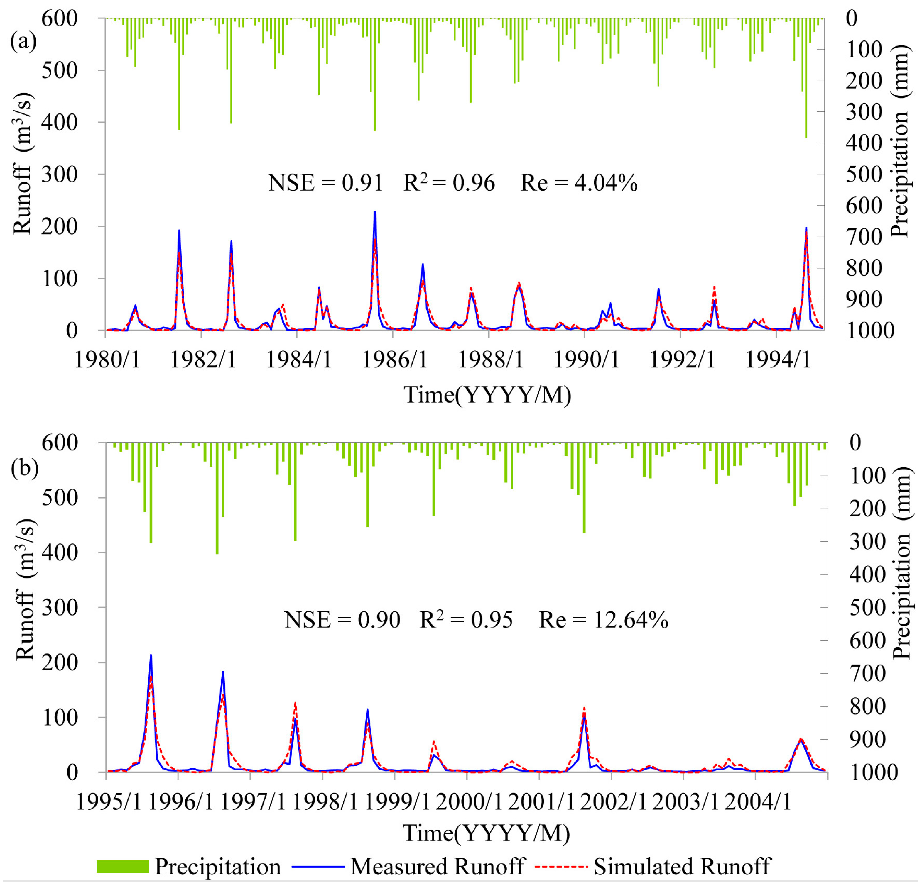
The SWAT model is calibrated and validated beforehand. The periods 1980–1994 and 1995–2004 were used as the calibration period and validation period, respectively. Yushi Reservoir runs after 2001 in the model. The simulated and measured monthly runoff are shown in Figure 2. The values of NSE and R² exceed 0.90 and 0.95, respectively. Re values are 4.04% and 12.64% in the calibration and validation. Therefore, the SWAT model is applicable for runoff prediction in this area.

4.2. Precipitation and Temperature Variations

After the 1980s, the Biliu River basin is affected by both climate change and human activities. The influence will exist in the future, and it is difficult to return to the natural state before 1980s. Therefore, the period after 1980s is used for precipitation and temperature downscaling. In addition, daily data are required for hydrological simulation. Thus, 1980–2004 is considered for downscaling since daily scale is not available after 2004. The climate model outputs in 1980–2004 and two future periods, 2016–2040 (near future) and 2041–2065 (far future), are utilized. Precipitation and temperature of the two future periods are downscaled respectively on the basis of 1980–2004 data. The output of the GCMs is bias corrected according to the observation in the historically period, and the same bias correction approach is applied to the output of GCMs in the future.

4.2.1. Temperature Variations

Two time periods, 1985–1994 and 1995–2004, were utilized to validate the morphing method for temperature downscaling. The downscaled temperature of 1995–2004 can be calculated using Equations (2)–(4). The downscaled temperature was compared with the historical observation in Figure 3 and Figure 4. The nine selected models are verified detail by detail because there is no scenario difference in the historical period.

Figure 3a compares the average annual mean temperatures of CMIP3 models. For BCCR_BCM2.0, CSIRO_MK3.0, and MIROC3.2m, the relative errors (Re) are −1.2%, −3.1%, and −4.8% respectively, and correlation coefficients (R²) all are larger than 0.60. Figure 3b compares monthly temperature variations. It can be seen that they agree well. Figure 4a shows the average annual mean temperature of the six models from CMIP5. Three of them—ACCESS1.0, CMCC-CM and MPI-ESM-MR—slightly overestimate the temperature with Re being 2.7%, 5.2%, and 3.4% respectively. The other three models slightly underestimate the temperature with Re of BCC-CSM1.1(m), CESM1(BGC), and CESM1(CAM5) being −3.4%, −2.3%, and −7.0% respectively. The R² of the six models all are larger than 0.60. Figure 4b shows the comparison of monthly temperature variations, and it can be seen that the downscaled temperatures agree well with observation. Overall, the morphing approach shows acceptable performance in the temperature downscaling.

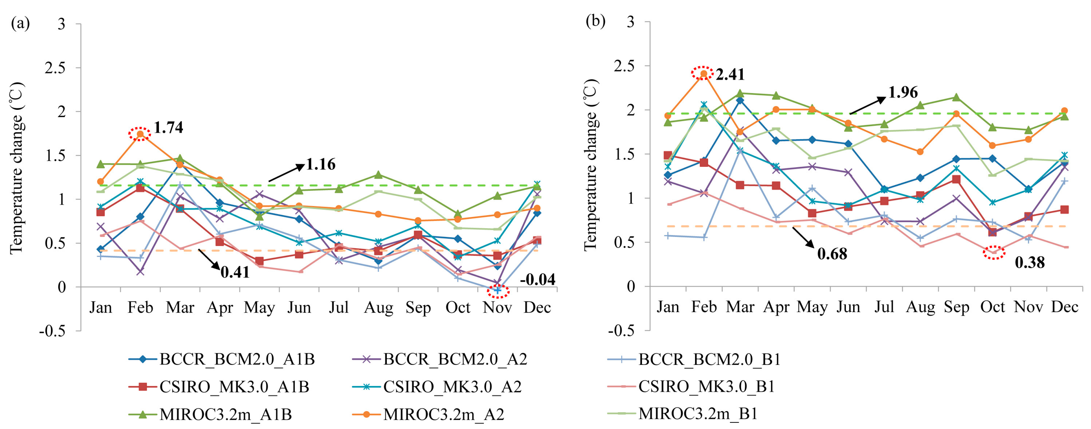
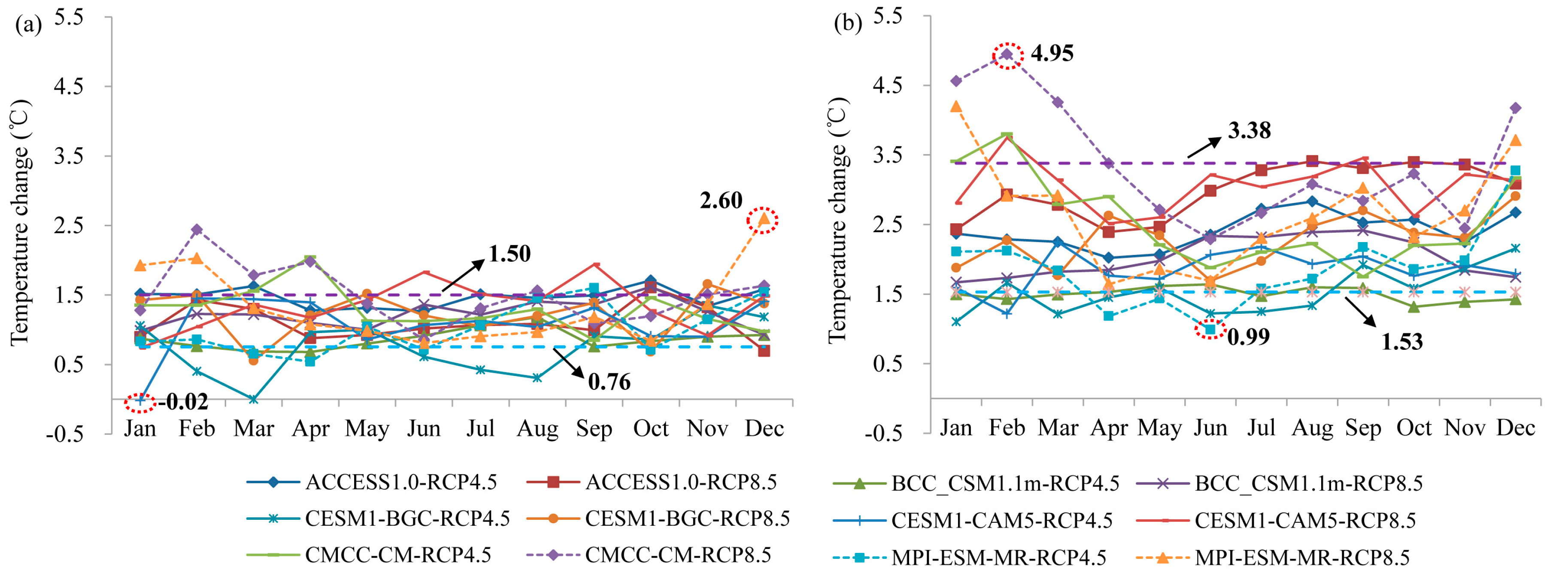
The annual mean temperature changes relative to 1980–2004 period are shown in Figure 5 and Figure 6. The horizontal dash lines refer to the maximum and minimum multi-year mean temperature changes, which show the ranges of change uncertainty, and can be calculated by Equations (8) and (9).

$$z_{\mathrm{MAX}}=\max \left\{\frac{1}{Y}{\displaystyle \sum _{j=1}^Y\mathrm{\Delta }{z}_i^j},i=1,2,\cdots ,k\right\}$$

(8)

$$z_{\mathrm{MIN}}=\min \left\{\frac{1}{Y}{\displaystyle \sum _{j=1}^Y\mathrm{\Delta }{z}_i^j},i=1,2,\cdots ,k\right\}$$

(9)

where $z_{\mathrm{MAX}}$ and $z_{\mathrm{MIN}}$ represent the maximum and minimum multi-year mean changes, respectively; $\mathrm{\Delta }{z}_i^j$ is the absolute or fractional changes in annual mean climate for year j based on the ith scenario; Y is the number of years and k is the number of scenarios.

As shown in Figure 5 and Figure 6, the annual mean temperature increases under all of the CMIP3 and CMIP5 scenarios. The annual mean temperature changes range from 0.41 to 1.16 °C under CMIP3 and range from 0.76 to 1.50 °C under CMIP5 in 2016–2040. The temperatures under all of the CMIP3 and CMIP5 scenarios increase even more in 2041–2065 than in 2016–2040, and the increases range from 0.68 to 1.96 °C under CMIP3 and range from 1.53 to 3.38 °C under CMIP5. Overall, future temperature increases range from 0.41 to 1.50 °C in 2016–2040 and 0.68 to 3.38 °C in 2041–2065 relative to 1980–2004 period on the basis of the selected scenarios. The results imply that temperatures are likely to increase in the future and increase more in the far future than in the near future. Moreover, temperature increases more under CMIP5 than under CMIP3.

The temperature differences between emission scenarios are also compared. Among A1B, A2, and B1, the increase in temperature from largest to smallest is A1B > A2 > B1 on the basis of BCCR_BCM2.0 and MIROC3.2m in both future periods, while it is A2 > A1B > B1 based on CSIRO_MK3.0. In addition, it is found that the temperature increases more in RCP8.5 than in RCP4.5 under all the models in both future periods except ACCESS1.0 in 2016–2040. This implies that climate emission scenarios are closely associated with temperature.

4.2.2. Precipitation Variations

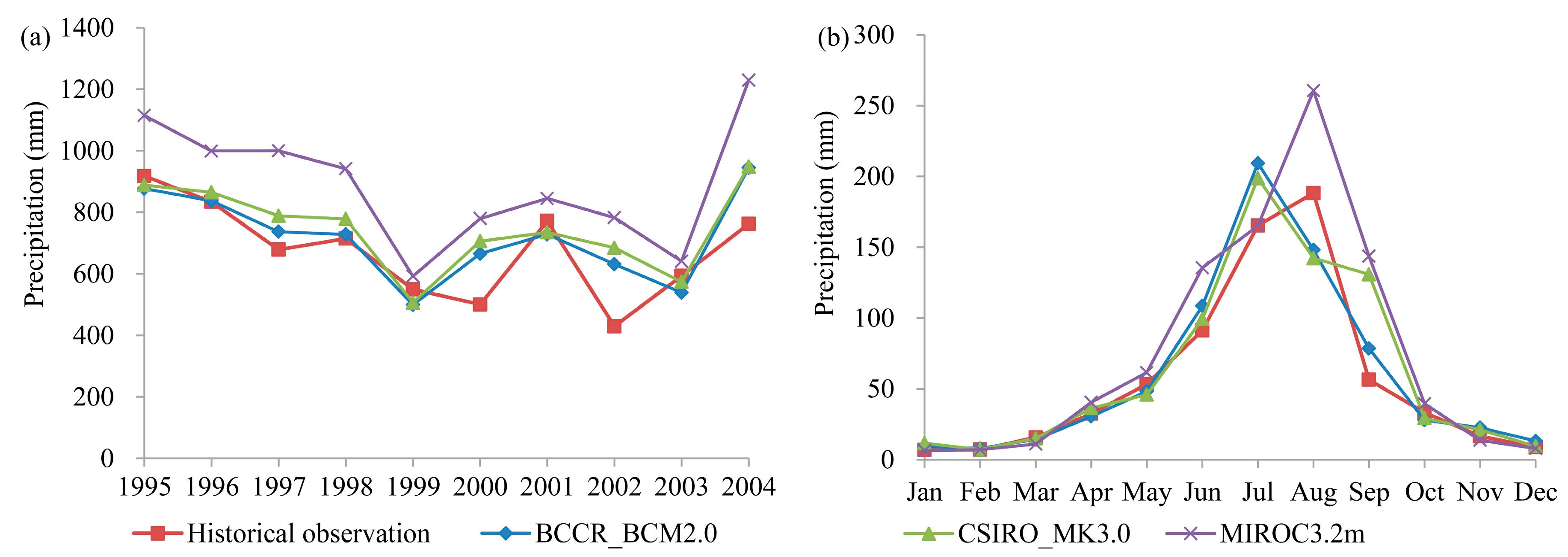
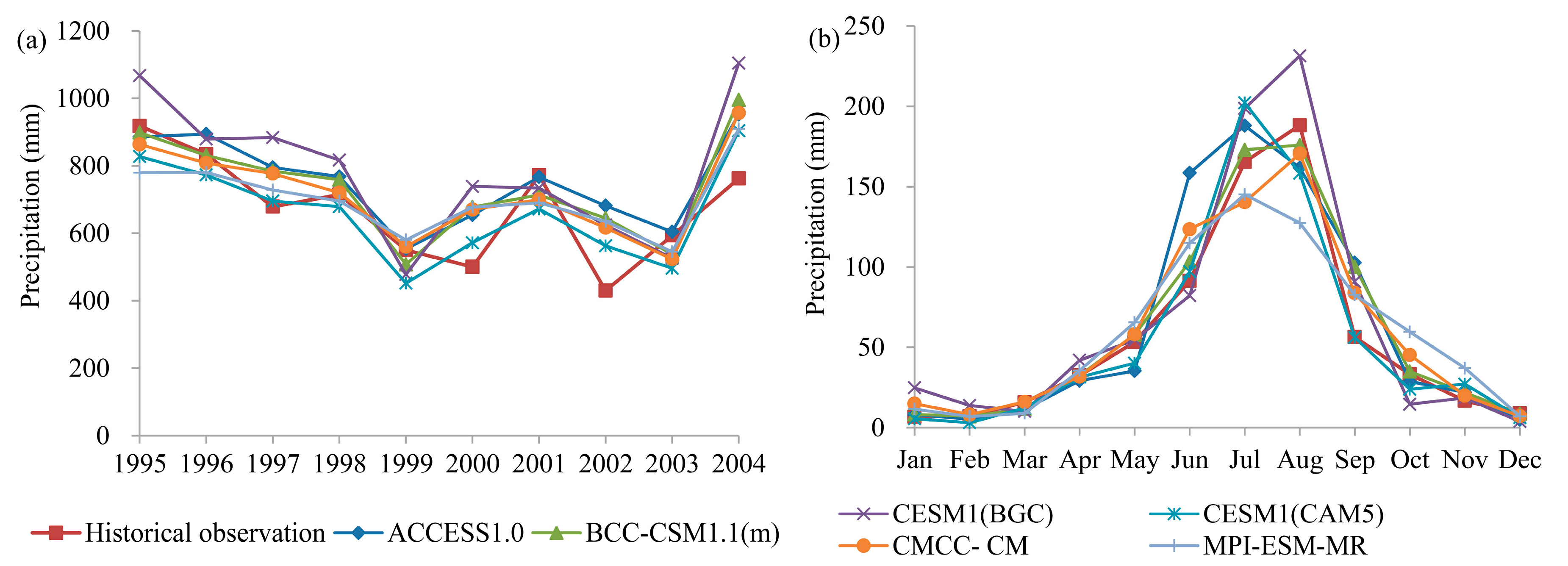
Similar to the temperature downscaling validation, two time periods, 1985–1994 and 1995–2004, were used to validate the applicability of the morphing method for precipitation downscaling. Downscaled precipitation of 1995–2004 can be calculated by Equation (1). The downscaled precipitation is compared with the historical observation precipitation to verify its accuracy in Figure 7 and Figure 8.

Figure 7a compares the annual precipitation of CMIP3 models. For BCCR_BCM2.0, CSIRO_MK3.0 and MIROC3.2m, Re are 6.4%, 10.7% and 32.2% respectively, and R² are larger than 0.72. Figure 7b compares monthly precipitation variations. It can be seen that they agree well. Figure 8a shows the average annual precipitation of the six models from CMIP5. Only one of them—CESM1(CAM5)—slightly underestimated the precipitation (Re is −1.8%). The other five models all overestimate the precipitation. The Re of ACCESS1.0, BCC-CSM1.1(m), CMCC-CM, CESM1(BGC), and MPI-ESM-MR are 11.9, 8.8, 6.5, 16.3, and 4.0% respectively. The R² of the six models all are larger than 0.70. Figure 8b shows a comparison of monthly precipitation variations. The fitting result is accurate: R² values are larger than 0.93. Overall, the morphing results basically meet the downscaling requirements, which demonstrates that the morphing method is valid for precipitation downscaling.

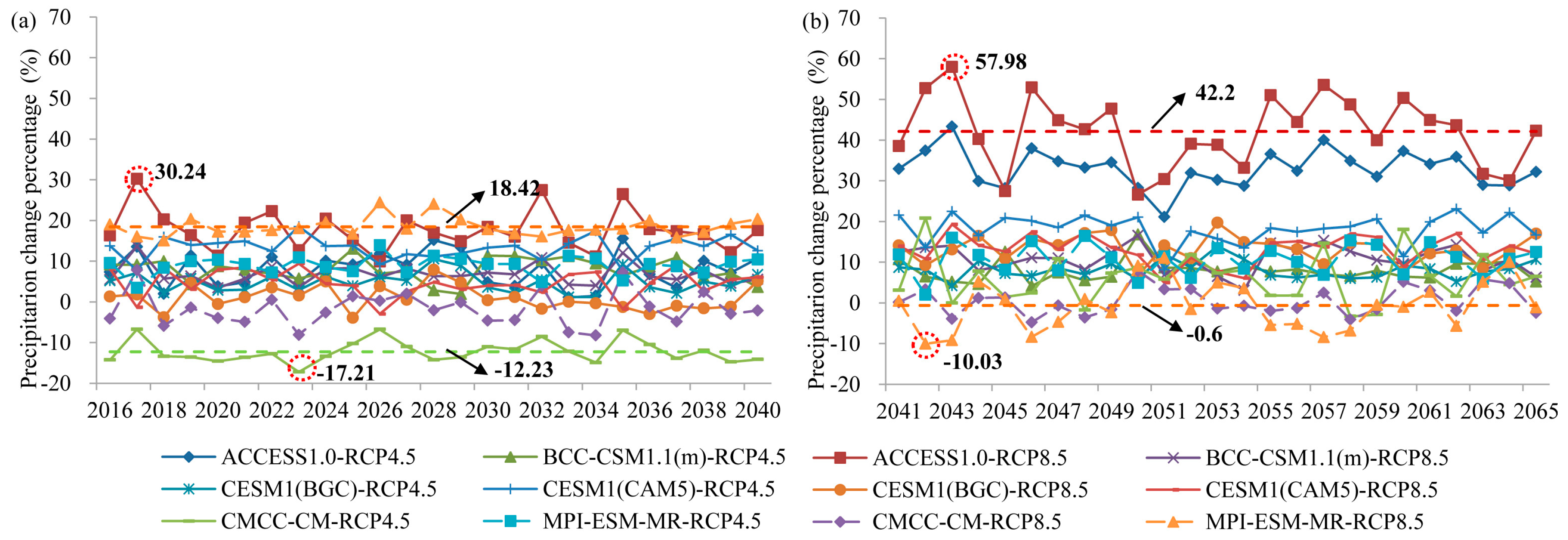
The annual mean change percentages relative to 1980–2004 period are shown in Figure 9 and Figure 10. The horizontal dash lines refer to the maximum and minimum multi-year mean precipitation change percentages, which show the ranges of change uncertainty, as calculated by Equations (8) and (9).

As shown in Figure 9, annual precipitation increases under most of the CMIP3 scenarios except CSIRO_MK3.0 (B1). The mean annual change percentage ranges from −2.13% to 21.85% in 2016–2040. The range is slightly smaller in 2041–2065, which ranges from −4.08% to 14.65%. The difference of MIROC3.2m (B1) in the two future periods is the greatest, followed by BCCR_BCM2.0 (A2) and MIROC3.2m (A1B). The other six scenarios differ by less than ±5%. This implies that future precipitation is likely to increase, with similar changes in the near future and far future.

As shown in Figure 10, annual precipitation increases under most of the CMIP5 scenarios except CMCC-CM (RCP4.5 and RCP8.5) in 2016–2040 and MPI-ESM-MR (RCP8.5) in 2041–2065. The annual mean change percentage ranges from −12.23% to 18.42% in 2016–2040. The range is significantly wider in 2041–2065, which ranges from −0.6% to 42.2%. Compared to the results in 2016–2040, the precipitation change percentage in 2041–2065 decreases only under MPI-ESM-MR (RCP8.5), while the other 11 scenarios all increase. This implies that future precipitation is likely to increase. Moreover, precipitation in the far future is likely to increase more significantly than in the near future. On the other hand, future precipitation decreases under a few scenarios, which reveals the uncertainties of future precipitation. Overall, future precipitation changes range from −12.23% to 21.85% in 2016–2040 and −4.08% to 42.2% in 2041–2065 relative to 1980–2004 period on the basis of the selected scenarios.

The precipitation differences between emission scenarios are also compared. Among A1B, A2, and B1, the increase in precipitation from largest to smallest is A1B > A2 > B1 on the basis of CSIRO_MK3.0 in both future periods. However, the pattern is not obvious under the other two models. In addition, it is found that half of the models have larger change percentages under RCP8.5 while the other half have larger change percentages under RCP4.5. This implies that climate emission scenarios are not so closely associated with precipitation.

The historical annual series of 1958–2011 data are considered as the baseline to further analyze the precipitation variations. Compared to the historical mean annual precipitation of the baseline period (739.4 mm), the change percentages of the forecasted long series (2016–2065) are no more than ±10% under CMIP3 scenarios. Specifically, the forecasted mean annual precipitation decreases by 0.56, 1.77, and 8.3% under BCCR_BCM2.0 (B1), CSIRO_MK3.0 (A2), and CSIRO_MK3.0 (B1) respectively, while it increases under the other six CMIP3 scenarios. Among the 12 CMIP5 scenarios, the decline in precipitation only appears in the CMCC-CM model, with declines of 8.67% and 6.56% for RCP4.5 and RCP8.5, respectively. The maximum increase appears in the ACCESS1.0 model, while the other scenarios show smaller increases. The increased proportions of precipitation are mostly below 10%, with two exceptions: the ACCESS1.0 models for RCP4.5 and RCP8.5. A comparison of the results is shown in

Table 2. Mean annual precipitation and runoff in the historical period (1958–2011) and future period (2016–2065).

Climate Scenario	Precipitation (mm)	Runoff (mm)	Runoff Coefficient	Change Percentage (%)
				Precipitation	Runoff	Runoff Coefficient
Historical observation	739.43	275.43	0.37	-	-	-
BCCR_BCM2.0(A1B)	741.76	258.55	0.35	0.31	−6.13	−6.43
BCCR_BCM2.0(A2)	739.93	263.35	0.36	0.07	−4.39	−4.45
BCCR_BCM2.0(B1)	735.28	260.24	0.35	−0.56	−5.52	−4.98
CSIRO_MK3.0(A1B)	790.78	300.37	0.38	6.94	9.06	1.97
CSIRO_MK3.0(A2)	726.37	249.02	0.34	−1.77	−9.59	−7.97
CSIRO_MK3.0(B1)	678.03	217.10	0.32	−8.30	−21.18	−14.04
MIROC3.2m(A1B)	805.40	306.29	0.38	8.92	11.20	2.10
MIROC3.2m(A2)	760.50	276.14	0.36	2.85	0.26	−2.52
MIROC3.2m(B1)	793.18	300.71	0.38	7.27	9.18	1.78
ACCESS1.0 (RCP4.5)	841.15	331.45	0.39	13.76	20.34	5.79
ACCESS1.0 (RCP8.5)	909.90	398.39	0.44	23.05	44.64	17.54
BCC-CSM1.1(m)(RCP4.5)	752.82	261.36	0.35	1.81	−5.11	−6.80
BCC-CSM1.1(m)(RCP8.5)	759.89	269.18	0.35	2.77	−2.27	−4.90
CESM1(BGC) (RCP4.5)	741.93	254.00	0.34	0.34	−7.78	−8.09
CESM1(BGC) (RCP8.5)	748.55	264.06	0.35	1.23	−4.13	−5.30
CESM1(CAM5) (RCP4.5)	807.84	307.95	0.38	9.25	11.81	2.34
CESM1(CAM5) (RCP8.5)	761.03	268.87	0.35	2.92	−2.38	−5.15
CMCC-CM (RCP4.5)	675.31	204.83	0.30	−8.67	−25.63	−18.57
CMCC-CM (RCP8.5)	690.96	204.70	0.30	−6.56	−25.68	−20.47
MPI-ESM-MR (RCP4.5)	766.74	266.63	0.35	3.69	−3.20	−6.64
MPI-ESM-MR (RCP8.5)	756.81	248.18	0.33	2.35	−9.90	−11.97

.

4.3. Future Evaporation and Runoff Conditions under Climate Changes

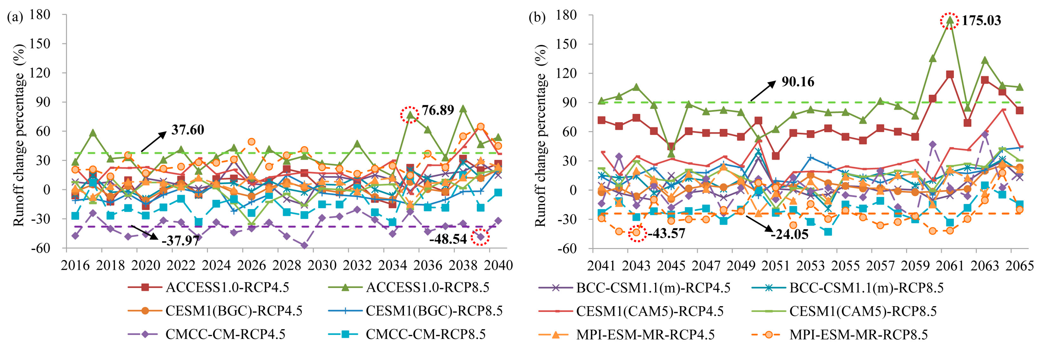
The annual evaporation and runoff of the 21 scenarios in the two future periods are predicted by the SWAT model using the downscaled daily precipitation and temperature data. The predicted evaporation and runoff percentage differences relative to the 1980–2004 period are shown in Figure 11, Figure 12, Figure 13 and Figure 14, respectively. The horizontal dashed lines in the figures refer to the maximum and minimum multi-year mean evaporation and runoff change percentages, which can be calculated by Equations (8) and (9), show the ranges of change uncertainty.

Figure 11 shows the annual evaporation changes under CMIP3 scenarios. The annual mean change percentage ranges from −1.09% to 5.50% in 2016–2040. The range is slightly wider in 2041–2065, which ranges from −0.85% to 7.21%. Figure 12 shows the annual evaporation changes under CMIP5 scenarios. The annual mean change percentage ranges from −2.05% to 8.90% in 2016–2040. The range is slightly smaller in 2041–2065, which ranges from 5.10% to 12.55%. Compared to the results in 2016–2040, the annual evaporation change percentages are similar under CMIP3 but much larger under CMIP5. Future annual evaporation all increase except CSIRO_MK3.0 (B1) for two future periods and CMCC-CM (RCP4.5) for 2016–2040. Overall, future evaporation changes range from −2.05% to 8.90% in 2016–2040 and −2.70% to 12.55% in 2041–2065 relative to 1980–2004 period on the basis of the selected scenarios. The increase in future evaporation is mainly caused by the rising temperature.

Figure 13 shows the annual runoff changes under CMIP3 scenarios. The annual mean change percentage ranges from −13.35% to 46.59% in 2016–2040. The range is slightly smaller in 2041–2065, which ranges from −19.39% to 25.47%. The difference of MIROC3.2m (B1) in the two future periods is the greatest, followed by MIROC3.2m (A1B) and BCCR_BCM2.0 (A2). The other six scenarios differ by less than ±10%.

Figure 14 shows the annual runoff changes under CMIP5 scenarios. The annual mean change percentage ranges from −37.97% to 37.60% in 2016–2040. The range is significantly wider in 2041–2065, which ranges from −24.05% to 90.16%. Compared to the results in 2016–2040, the runoff change percentage in 2041–2065 decreases most under MPI-ESM-MR (RCP8.5), which is also the only scenario under which precipitation decreases. Meanwhile, runoff slightly decreases under BCC-CSM1.1(m) (RCP4.5), CMCC-CM (RCP8.5), and MPI-ESM-MR (RCP4.5), while under the other eight scenarios runoff increases. Overall, future runoff changes range from −37.97% to 46.59% in 2016–2040 and −24.05% to 90.16% in 2041–2065 relative to 1980–2004 period on the basis of the selected scenarios.

This implies that changes in future runoff are greater than changes in precipitation under both CMIP3 and CMIP5. However, future runoff changes are relatively similar in the near future and far future under CMIP3, but are much more severe in the far future than in the near future under CMIP5. In addition, the ranges of change in runoff under CMIP5 are much wider than under CMIP3.

Among A1B, A2, and B1, the change of runoff from largest to smallest is A1B > A2 > B1 under CSIRO_MK3.0 in both future periods. However, the pattern is not obvious under the other two models. In addition, it is found that half of the models have larger change percentages under RCP8.5 while the other half have larger change percentages under RCP4.5. The situation is just like that of the precipitation changes, but with different change percentages. This implies that climate emission scenarios are also not so closely associated with runoff.

The forecasted long series (2016–2065) of runoff is compared with the baseline series (1958–2011) in order to thoroughly analyze the future runoff changes which are more practical for decision makers. Compared to the historical mean annual runoff (275.43 mm), the mean annual runoff decreases under five CMIP3 scenarios while it increases under the other four scenarios. Specifically, the scenarios under which mean annual runoff increases include MIROC3.2m for A1B, A2, and B1, and CSIRO_MK3.0 (A1B). The forecasted mean annual runoff increases by up to 11.20% under MIROC3.2m (A1B), while it decreases by up to 21.18% under CSIRO_MK3.0 (B1); this is because the precipitation under these scenarios increases the most and decreases the most respectively. Among the 12 CMIP5 scenarios, runoffs increase in the ACCESS1.0 model for RCP4.5 and RCP8.5, as well as the CESM1 (CAM5) model for RCP4.5, while the other scenarios all have a decline in runoff. Runoff increases by up to 20.34% and 44.64% under the ACCESS1.0 model for RCP4.5 and RCP8.5 respectively, mainly because their precipitation increases the most. On the other hand, runoffs of the CMCC-CM model decrease by up to 25.63% and 25.68% for RCP4.5 and RCP8.5 respectively, which is because the precipitation decreases the most. A comparison of the results is shown in Table 2. Overall, compared to the baseline series, the runoff decreases under two-thirds of the selected scenarios including five CMIP3 scenarios and nine CMIP5 scenarios.

5. Discussion

The morphing results are affected by the characteristics of the ‘baseline climate’. However, the morphing results meet the downscaling requirements in this study; in addition, the method is simple and requires only a small computation volume. That is the reason why morphing is utilized in this study.

Compared to 1980–2004 period, both temperature and precipitation increase under most of the scenarios, and they both increase more in the far future than in the near future under both CMIP3 and CMIP5. Moreover, the temperature increases more under CMIP5 than under CMIP3 scenarios. Several studies have shown that CMIP5 presents warmer and wetter predictions [19,20]. Meanwhile, the ranges of change in both precipitation and runoff under CMIP5 are much wider than under CMIP3, which indicates that the selected CMIP5 scenarios are more effective in capturing future runoff uncertainties than the selected CMIP3 scenarios. In addition, the results imply that climate emission scenarios are closely associated with temperature but not so closely associated with precipitation and runoff.

As shown in Table 2, the runoff changes differ from precipitation changes. In most scenarios (15 of the 21 chosen scenarios), the decline in precipitation results in a more significant decline in runoff, while the increase in precipitation results in less increase in runoff. This implies that whether the precipitation increases or decreases, part of the water is failed to form runoff. There are six exceptions when the annual precipitation is more than 790 mm and the increase in runoff is larger than that of precipitation. The six exceptions include three CMIP3 scenarios (CSIRO_MK3.0 (A1B), MIROC3.2m (A1B), and MIROC3.2m (B1)) and three CMIP5 scenarios (the ACCESS1.0 model for RCP4.5, RCP8.5, and CESM1(CAM5) (RCP4.5)), which are the same as the six runoff increase scenarios. Precipitation supplements the soil moisture content when precipitation reaches or exceeds a certain amount. After the soil moisture content is saturated, most of the remaining precipitation forms runoff [31]. The runoff coefficient of precipitation thus increases (as show in Table 2), which may result in the larger increase in runoff than precipitation.

The relatively low flow conditions of the 1980–2004 period may partly result in the decline in future runoff when compared to the baseline series. Three impact factors are further analyzed. First, Yushi Reservoir supplies water to the outside of the basin, about 46 million m³ each year (about 22.1 mm). This is one cause of the decline in runoff. Second, compared to 1980–2004 period, the simulated future evaporation increased under all the selected scenarios in both future periods except CSIRO_MK3.0 (B1) and CMCC-CM (RCP4.5) with slightly decreases. Evaporation increases greater in the far future than in the near future, which is the same to the temperature increase pattern. The increase in evaporation caused by the rising temperature is another cause of the decline in future runoff. Third, on the basis of water balance in the basin, the upstream water consumption, such as farmers getting water from the stream for irrigation, may be another factor which affects future runoff. Unlike the former two factors, the amount of upstream water consumptions is relatively small, and the impact on runoff is not obvious in these scenarios.

Acknowledging the uncertainty of the simulated runoff using the GCMs in the future [13,20,21,38], it is hard to give an accurate estimate about how much water the reservoir will have. However, the results in this study do show that the runoff in the future could decrease. This decrease could provide important information for the long-term planning of the development of this region. At present, the study region has a few factories that consume much water every year, and the water demand may increase in the future. In addition, the water used for irrigation could also increase in the future. The decreasing runoff (as shown in this study) suggests that this region may suffer from water shortages if industrial and irrigation demands keep increasing in the future. This information is beneficial for regional sustainable development, and indicates that possible adaption measures (e.g., building water transfer projects) should be taken in advance to adapt to climate change.

6. Conclusions

This study investigated the variations of future climate and water resources availability in an important river basin (the Biliu River basin) in northeast China. We found that both temperature and precipitation increase under most of the CMIP3 and CMIP5 scenarios, and CMIP5 shows higher temperature and wider ranges of changes in precipitation and runoff than CMIP3. We also found that the evaporation could increase and the runoff could decrease in the future. The decline in runoff may aggravate water shortages in the Biliu River basin, which may influence the water security in nearby big cities. The results provide very important information for water resources planning and management in this region and could have important implications to the regional sustainable development.

The uncertainties caused by the downscaling method and hydrological model, which are not considered in this article, require further research. In addition, the impact of human activities on future runoff, as well as the comprehensive impact of change conditions, also requires further research. Furthermore, it is necessary to combine these results with the analysis of reservoir regulation rules in order to use this information to make an informed decision about the future water availability for this reservoir.

References

1. Menzel, L.; Bürger, G. Climate change scenarios and runoff response in the Mulde catchment (Southern Elbe, Germany). J. Hydrol. 2002, 267, 53–64. [Google Scholar] [CrossRef]
2. Hawkins, E.; Sutton, R. The potential to narrow uncertainty in regional climate predictions. Bull. Am. Meteorol. Soc. 2009, 90, 1095–1107. [Google Scholar] [CrossRef]
3. Woldemeskel, F.M.; Sharma, A.; Sivakumar, B.; Mehrotra, R. A framework to quantify GCM uncertainties for use in impact assessment studies. J. Hydrol. 2014, 519, 1453–1465. [Google Scholar] [CrossRef]
4. Intergovernmental Panel on Climate Change (IPCC). Climate Change 2007: The Physical Science Basis. Contribution of Working Group I to the Fourth Assessment Report of the Intergovernmental Panel on Climate Change; Cambridge Universty Press: New York, NY, USA, 2007. [Google Scholar]
5. Sivakumar, B. Global climate change and its impacts on water resources planning and management: Assessment and challenges. Stoch. Environ. Res. Risk Assess. 2011, 25, 583–600. [Google Scholar] [CrossRef]
6. Towler, E.; Rajagopalan, B.; Gilleland, E.; Summers, R.S.; Yates, D.; Katz, R.W. Modeling hydrologic and water quality extremes in a changing climate: A statistical approach based on extreme value theory. Water Resour. Res. 2010, 46, W11504. [Google Scholar] [CrossRef]
7. Belcher, S.E.; Hacker, J.N.; Powell, D.S. Constructing design weather data for future climates. Build. Serv. Eng. Res. Technol. 2005, 26, 49–61. [Google Scholar] [CrossRef]
8. Milzow, C.; Burg, V.; Kinzelbach, W. Estimating future ecoregion distributions within the Okavango Delta Wetlands based on hydrological simulations and future climate and development scenarios. J. Hydrol. 2010, 381, 89–100. [Google Scholar] [CrossRef]
9. Chen, S.T.; Yu, P.S.; Tang, Y.H. Statistical downscaling of daily precipitation using support vector machines and multivariate analysis. J. Hydrol. 2010, 385, 13–22. [Google Scholar] [CrossRef]
10. Zhang, C.; Zhu, X.P.; Fu, G.T.; Zhou, H.C.; Wang, H. The impacts of climate change on water diversion strategies into a water deficit reservoir. J. Hydroinform. 2014, 16, 872–889. [Google Scholar] [CrossRef]
11. Taylor, K.E.; Stouffer, R.J.; Meehl, G.A. A summary of the CMIP5 experiment design. Bull. Am. Meteorol. Soc. 2012, 93, 485–498. [Google Scholar] [CrossRef]
12. Brekke, L.D.; Dettinger, M.D.; Maurer, E.P.; Anderson, M. Significance of model credibility in estimating climate projection distributions for regional hydroclimatological risk assessments. Clim. Chang. 2008, 89, 371–394. [Google Scholar] [CrossRef]
13. Hoang, L.P.; Lauri, H.; Kummu, M.; Koponen, J.; van Vliet, M.T.H.; Supit, I.; Leemans, R.; Kabat, P.; Ludwig, F. Mekong River flow and hydrological extremes under climate change. Hydrol. Earth Syst. Sci. 2016, 20, 3027–3041. [Google Scholar] [CrossRef]
14. Donat, M.G.; Lowry, A.L.; Alexander, L.V.; O’Gorman, P.A.; Maher, N. More extreme precipitation in the world’s dry and wet regions. Nat. Clim. Chang. 2016, 6, 508–513. [Google Scholar] [CrossRef]
15. Wang, G.L.; Wang, D.G.; Trenberth, K.E.; Erfanian, A.; Yu, M.; Bosilovich, M.G.; Parr, D.T. The peak structure and future changes of the relationships between extreme precipitation and temperature. Nat. Clim. Chang. 2017, 7, 268–274. [Google Scholar] [CrossRef]
16. Wang, X.Y.; Yang, T.; Li, X.L.; Shi, P.F.; Zhou, X.D. Spatio-temporal changes of precipitation and temperature over the Pearl River basin based on CMIP5 multi-model ensemble. Stoch. Environ. Res. Risk Assess. 2017, 31, 1077–1089. [Google Scholar] [CrossRef]
17. Koutroulis, A.G.; Grillakis, M.G.; Tsanis, I.K.; Papadimitriou, L. Evaluation of precipitation and temperature simulation performance of the CMIP3 and CMIP5 historical experiments. Clim. Dyn. 2016, 47, 1881–1898. [Google Scholar] [CrossRef]
18. Sun, Q.; Miao, C.; Duan, Q. Comparative analysis of CMIP3 and CMIP5 global climate models for simulating the daily mean, maximum, and minimum temperatures and daily precipitation over China. J. Geophys. Res. Atmos. 2015, 120, 4806–4824. [Google Scholar] [CrossRef]
19. Ayers, J.; Ficklin, D.L.; Stewart, I.T.; Strunk, M. Comparison of CMIP3 and CMIP5 projected hydrologic conditions over the Upper Colorado River Basin. Int. J. Climatol. 2016, 36, 3807–3818. [Google Scholar] [CrossRef]
20. Ficklin, D.L.; Letsinger, S.L.; Stewart, I.T.; Maurer, E.P. Assessing differences in snowmelt-dependent hydrologic projections using CMIP3 and CMIP5 climate forcing data for the western United States. Hydrol. Res. 2016, 47, 483–500. [Google Scholar] [CrossRef]
21. Shamir, E.; Megdal, S.B.; Carrillo, C.; Castro, C.L.; Chang, H.I.; Chief, K.; Corkhill, F.E.; Eden, S.; Georgakakos, K.P.; Nelson, K.M.; et al. Climate change and water resources management in the Upper Santa Cruz River, Arizona. J. Hydrol. 2015, 521, 18–33. [Google Scholar] [CrossRef]
22. Su, F.; Zhang, L.; Ou, T.; Chen, D.; Yao, T.; Tong, K.; Qi, Y. Hydrological response to future climate changes for the major upstream river basins in the Tibetan Plateau. Glob. Planet. Chang. 2016, 136, 82–95. [Google Scholar] [CrossRef]
23. Zhang, C.; Shoemaker, C.A.; Woodbury, J.D.; Cao, M.L.; Zhu, X.P. Impact of human activities on stream flow in the Biliu River basin, China. Hydrol. Process. 2013, 27, 2509–2523. [Google Scholar] [CrossRef]
24. Raje, D.; Mujumdar, P.P. Reservoir performance under uncertainty in hydrologic impacts of climate change. Adv. Water Resour. 2010, 33, 312–326. [Google Scholar] [CrossRef]
25. Vicuna, S.; Dracup, J.A.; Lund, J.R.; Dale, L.L.; Maurer, E.P. Basin-scale water system operations with uncertain future climate conditions: Methodology and case studies. Water Resour. Res. 2010, 46, W04505. [Google Scholar] [CrossRef]
26. Paiva, R.C.D.; Durand, M.T.; Hossain, F. Spatiotemporal interpolation of discharge across a river network by using synthetic SWOT satellite data. Water Resour. Res. 2015, 51, 430–449. [Google Scholar] [CrossRef]
27. Matin, M.A.; Bourque, C.P.A. Intra- and inter-annual variations in snow-water storage in data sparse desert-mountain regions assessed from remote sensing. Remote Sens. Environ. 2013, 139, 18–34. [Google Scholar] [CrossRef]
28. Glenn, J.; Tonina, D.; Morehead, M.D.; Fiedler, F.; Benjankar, R. Effect of transect location, transect spacing and interpolation methods on river bathymetry accuracy. Earth Surf. Process. Landf. 2016, 41, 1185–1198. [Google Scholar] [CrossRef]
29. CLIVAR Exchanges, World Climate Research Programme (WCRP). WCRP Coupled Model Intercomparison Project—Phase 5 (CMIP5); CLIVAR Exchanges No. 56, Vol. 16, No. 2; Indigo Press: Southampton, UK, 2011. [Google Scholar]
30. Van Vuuren, D.P.; Edmonds, J.; Kainuma, M.; Riahi, K.; Thomson, A.; Hibbard, K.A.; Hurtt, G.C.; Kram, T.; Krey, V.; Lamarque, J.F.; et al. The representative concentration pathways: An overview. Clim. Chang. 2011, 109, 5–31. [Google Scholar] [CrossRef]
31. Neitsch, S.L.; Arnold, J.G.; Kiniry, J.R.; Williams, J.R. Soil and Water Assessment Tool Theoretical Documentation; Version 2005; US Department of Agriculture (USDA) Agricultural Research Service (ARS): Temple, TX, USA, 2005.
32. Arnold, J.G.; Srinivasan, R.; Muttiah, R.S.; Williams, J.R. Large area hydrologic modeling and assessment. Part 1-Model development. J. Am. Water Resour. Assoc. 1998, 34, 1–17. [Google Scholar] [CrossRef]
33. U.S. Environmental Protection Agency (EPA). Protocols for Developing Nutrient TMDLs; Office of Water EPA 841-B-99-007; U.S. Environmental Protection Agency (EPA): Washington, DC, USA, 1999.
34. Marshall, E.; Randhir, T.O. Spatial modeling of land cover change and watershed response using Markovian cellular automata and simulation. Water Resour. Res. 2008, 44, W04423. [Google Scholar] [CrossRef]
35. Li, Z.; Liu, W.Z.; Zhang, X.C.; Zheng, F.L. Impacts of land use change and climate variability on hydrology in an agricultural catchment on the Loess Plateau of China. J. Hydrol. 2009, 377, 35–42. [Google Scholar] [CrossRef]
36. Van Griensven, A.; Meixner, T.; Grunwald, S.; Bishop, T.; Diluzio, M.; Srinivasan, R. A global sensitivity analysis tool for the parameters of multi-variable catchment models. J. Hydrol. 2006, 324, 10–23. [Google Scholar] [CrossRef]
37. Hao, F.H.; Cheng, T.G.; Yang, S.T. Non-Point Source Pollution Model; China Environmental Science Press: Beijing, China, 2006. [Google Scholar]
38. Mcsweeney, C.F.; Jones, R.G.; Booth, B.B.B. Selecting ensemble members to provide regional climate change information. J. Clim. 2012, 25, 7100–7121. [Google Scholar] [CrossRef]
Figure 1. The Biliu River basin.
Water 10 00126 g001
Figure 2. Simulated monthly runoff at Biliu River Reservoir station: (a) calibration period of 1980–1989; (b) validation period of 1990–1999.
Water 10 00126 g002
Figure 3. Comparison of the average downscaled temperature from CMIP3 using morphing and historical observation temperature series: (a) annual series; (b) monthly distribution.
Water 10 00126 g003
Figure 4. Comparison of the average downscaled temperature from CMIP5 using morphing and historical observation temperature series: (a) annual series; (b) monthly distribution.
Water 10 00126 g004
Figure 5. The forecasted temperature differences relative to 1980–2004 period under CMIP3: (a) the period 2016–2040; (b) the period 2041–2065.
Water 10 00126 g005
Figure 6. The forecasted temperature differences relative to 1980–2004 period under CMIP5: (a) the period 2016–2040; (b) the period 2041–2065.
Water 10 00126 g006
Figure 7. Comparison of the downscaled precipitation from CMIP3 using morphing and historical observation precipitation series: (a) annual series; (b) monthly distribution.
Water 10 00126 g007
Figure 8. Comparison of the downscaled precipitation from CMIP5 using morphing and historical observation precipitation series: (a) annual series; (b) monthly distribution.
Water 10 00126 g008
Figure 9. The forecasted precipitation change percentage relative to 1980–2004 period under CMIP3 (a) 2016–2040; (b) 2041–2065.
Water 10 00126 g009
Figure 10. The forecasted precipitation change percentage relative to 1980–2004 period under CMIP5 (a) 2016–2040; (b) 2041–2065.
Water 10 00126 g010
Figure 11. The forecasted evaporation change percentage relative to 1980–2004 period under CMIP3: (a) 2016–2040; (b) 2041–2065.
Water 10 00126 g011
Figure 12. The forecasted evaporation change percentage relative to 1980–2004 period under CMIP5: (a) 2016–2040; (b) 2041–2065.
Water 10 00126 g012
Figure 13. The forecasted runoff change percentage relative to 1980–2004 period under CMIP3: (a) 2016–2040; (b) 2041–2065.
Water 10 00126 g013
Figure 14. The forecasted runoff change percentage relative to 1980–2004 period under CMIP5: (a) 2016–2040; (b) 2041–2065.
Water 10 00126 g014