Improved Instruments and Methods for the Photographic Study of Spark-Induced Cavitation Bubbles


Abstract
1. Introduction
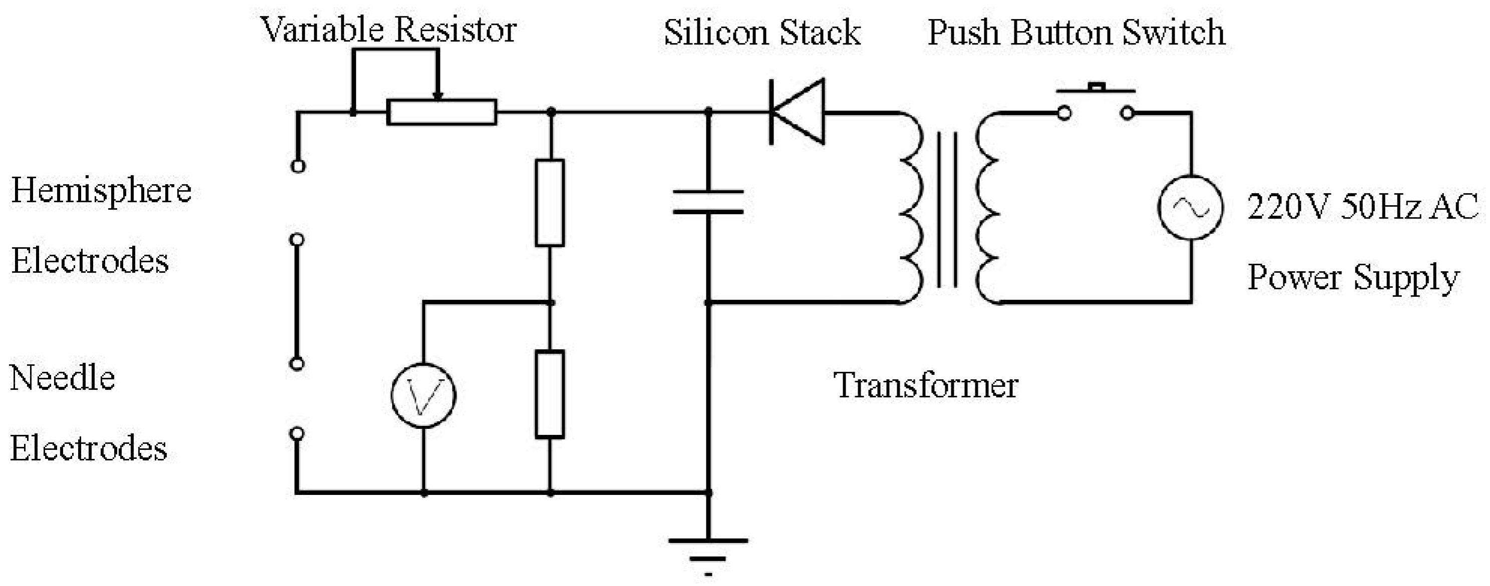
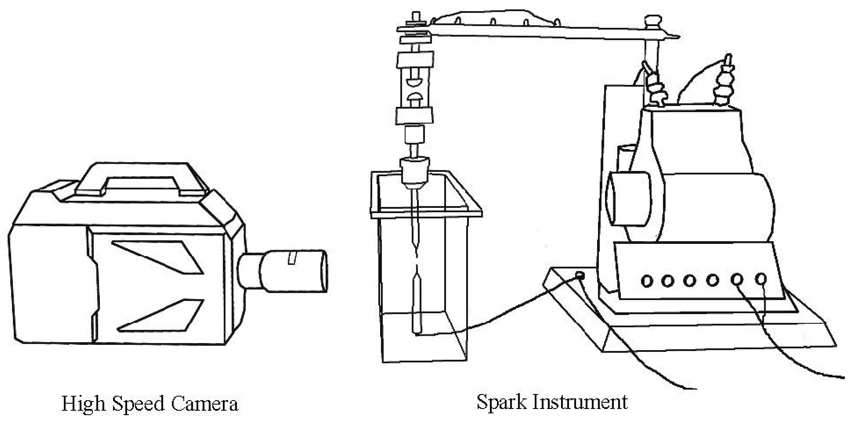
2. Materials and Methods
3. Results
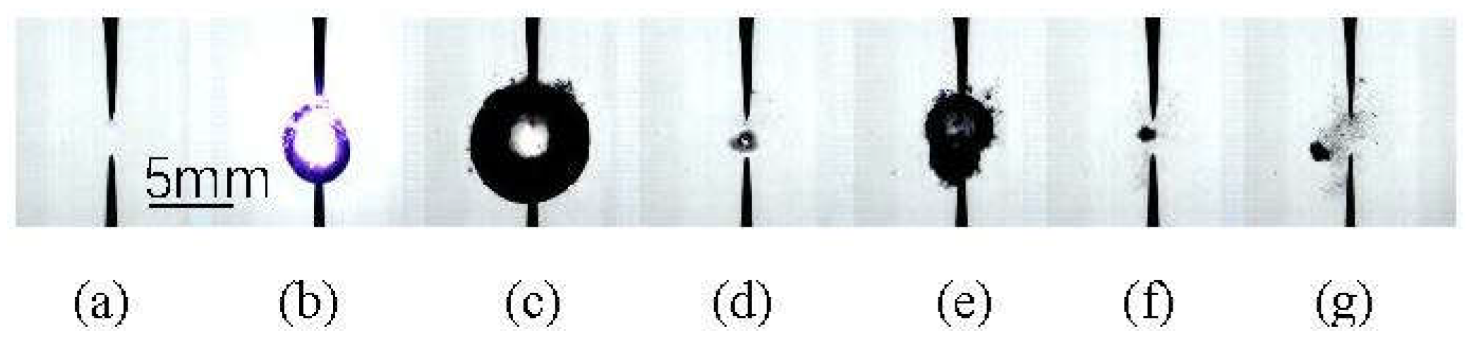
3.1. Photos
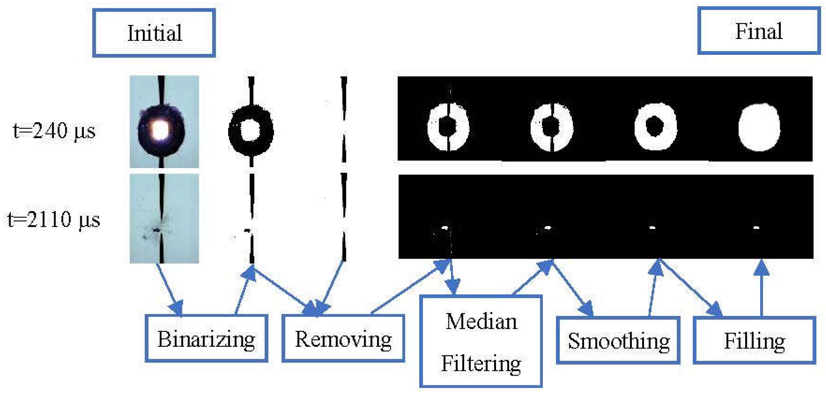
3.2. Image Processing Algorithm
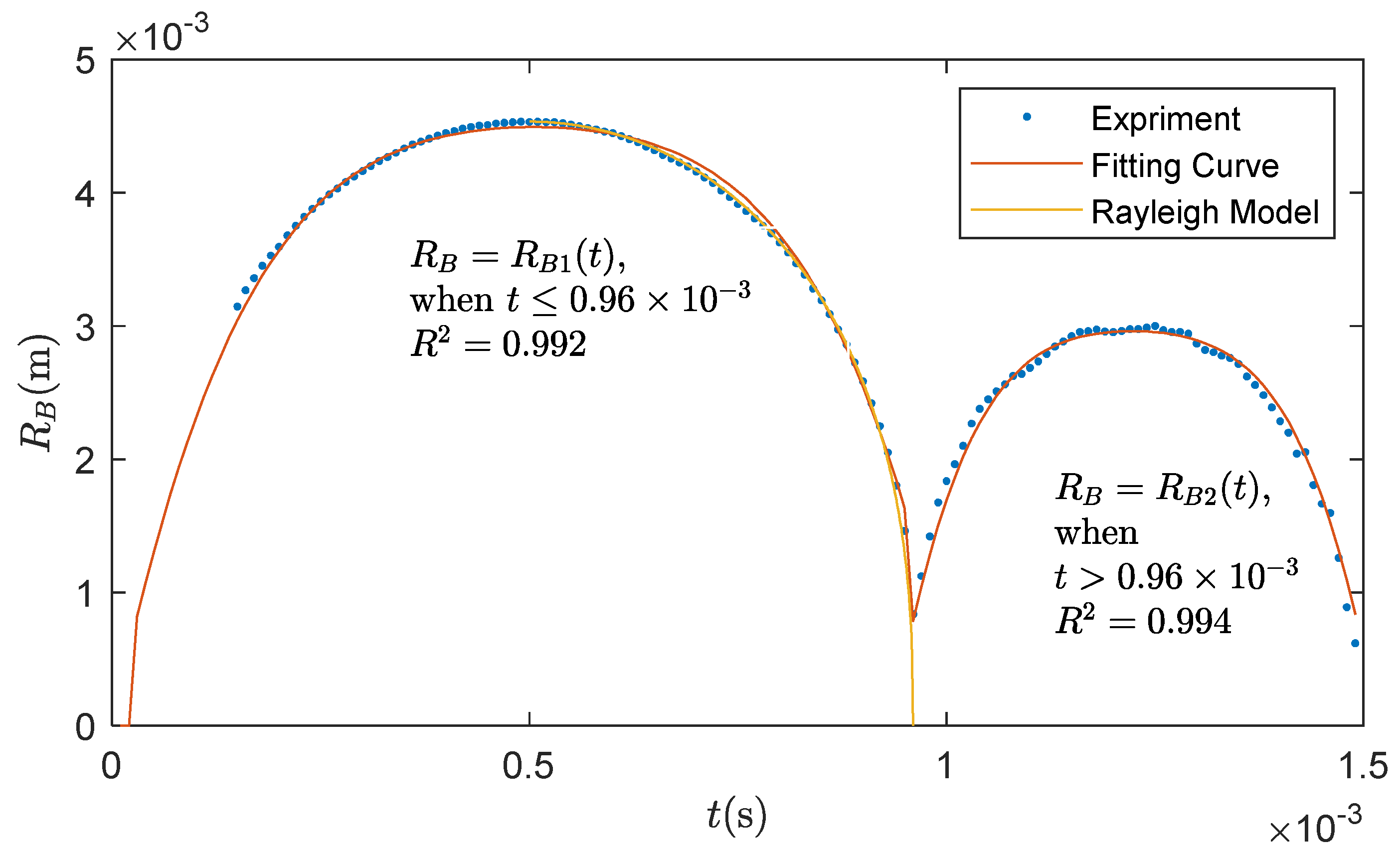
3.3. Radius Time History
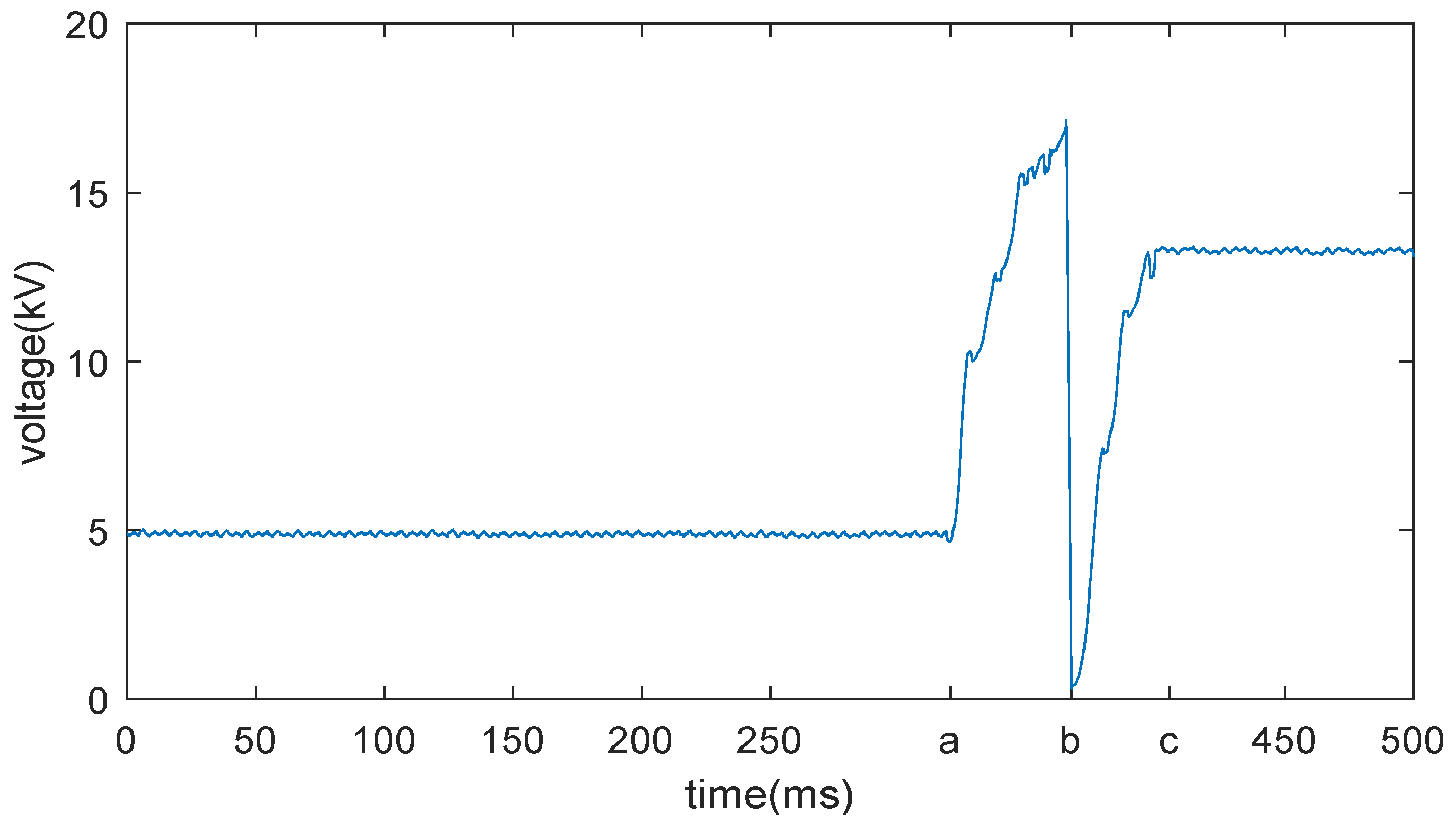
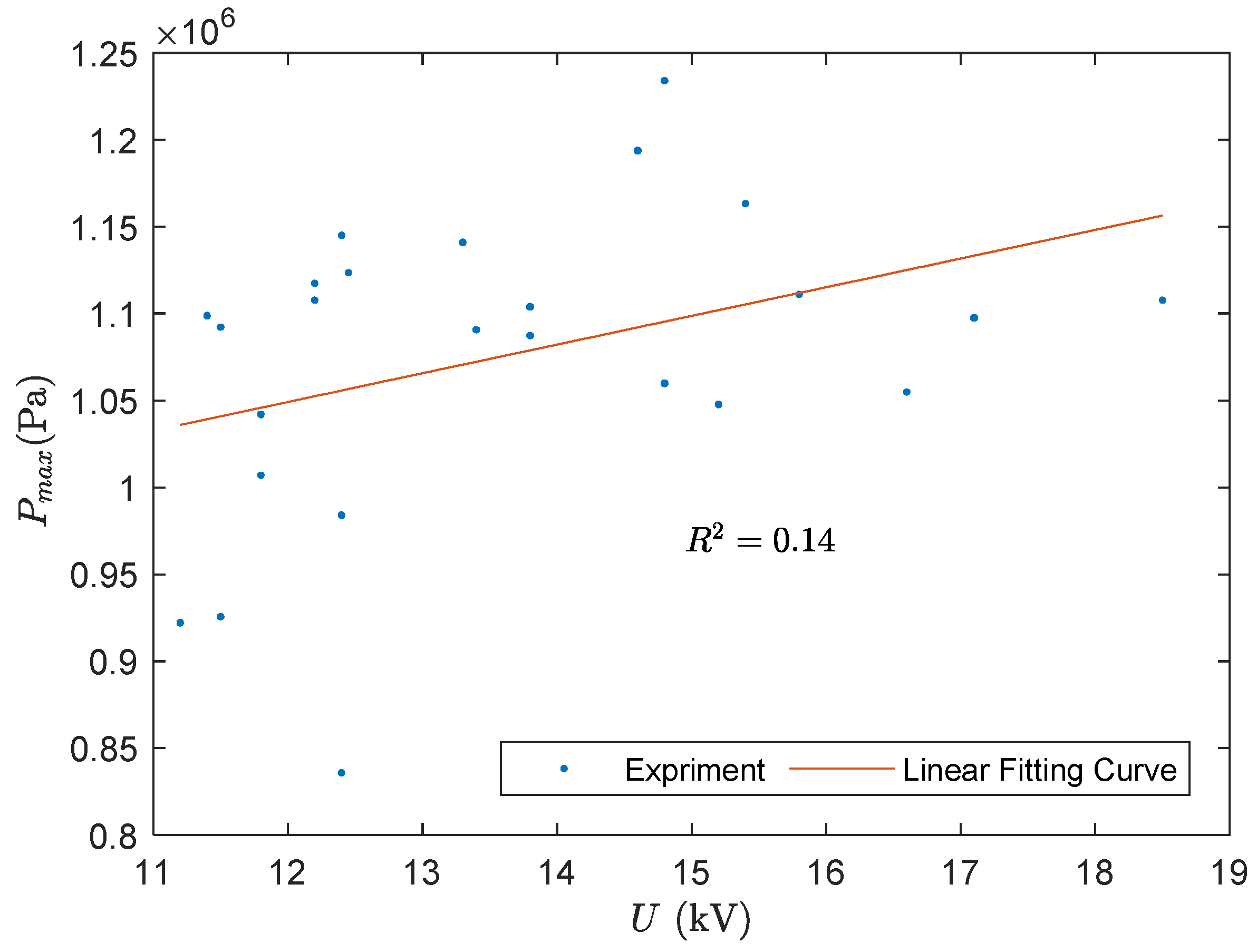
3.4. Breakdown Voltage and Bubble Radius
4. Discussion
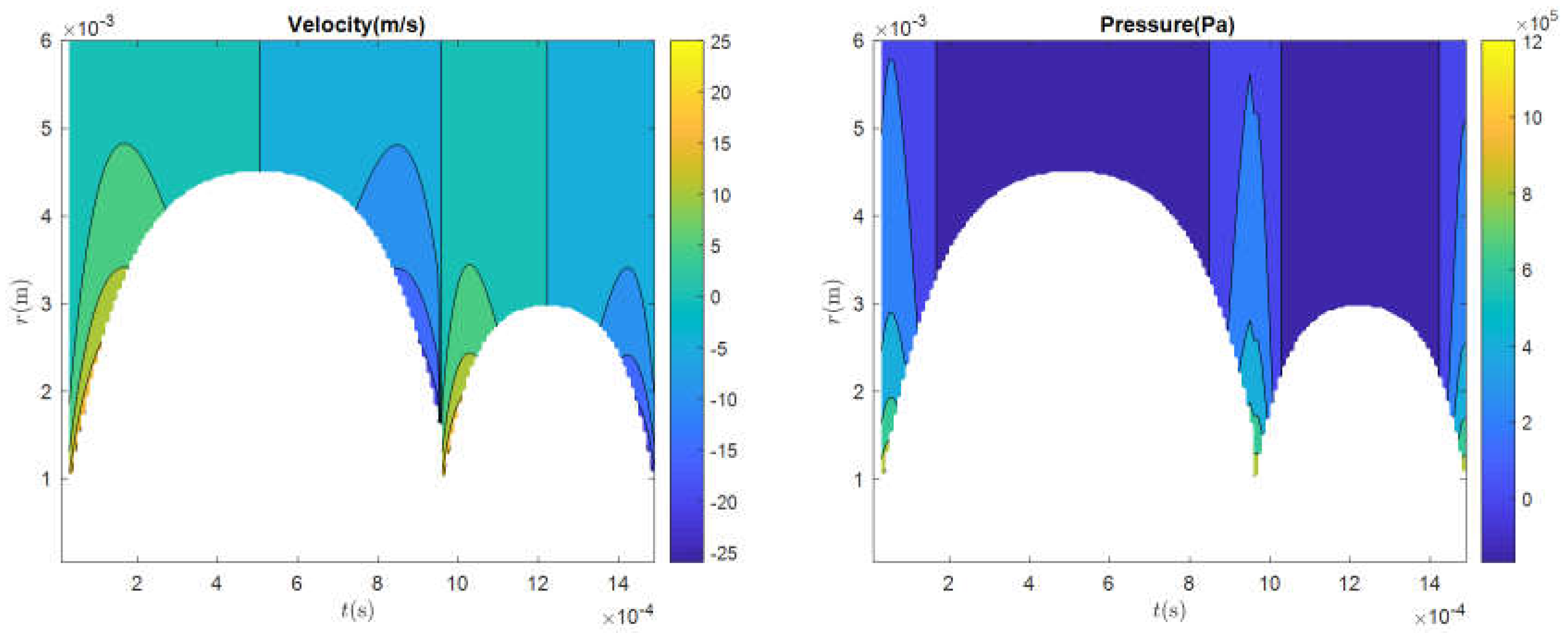
4.1. Single Bubble Dynamics
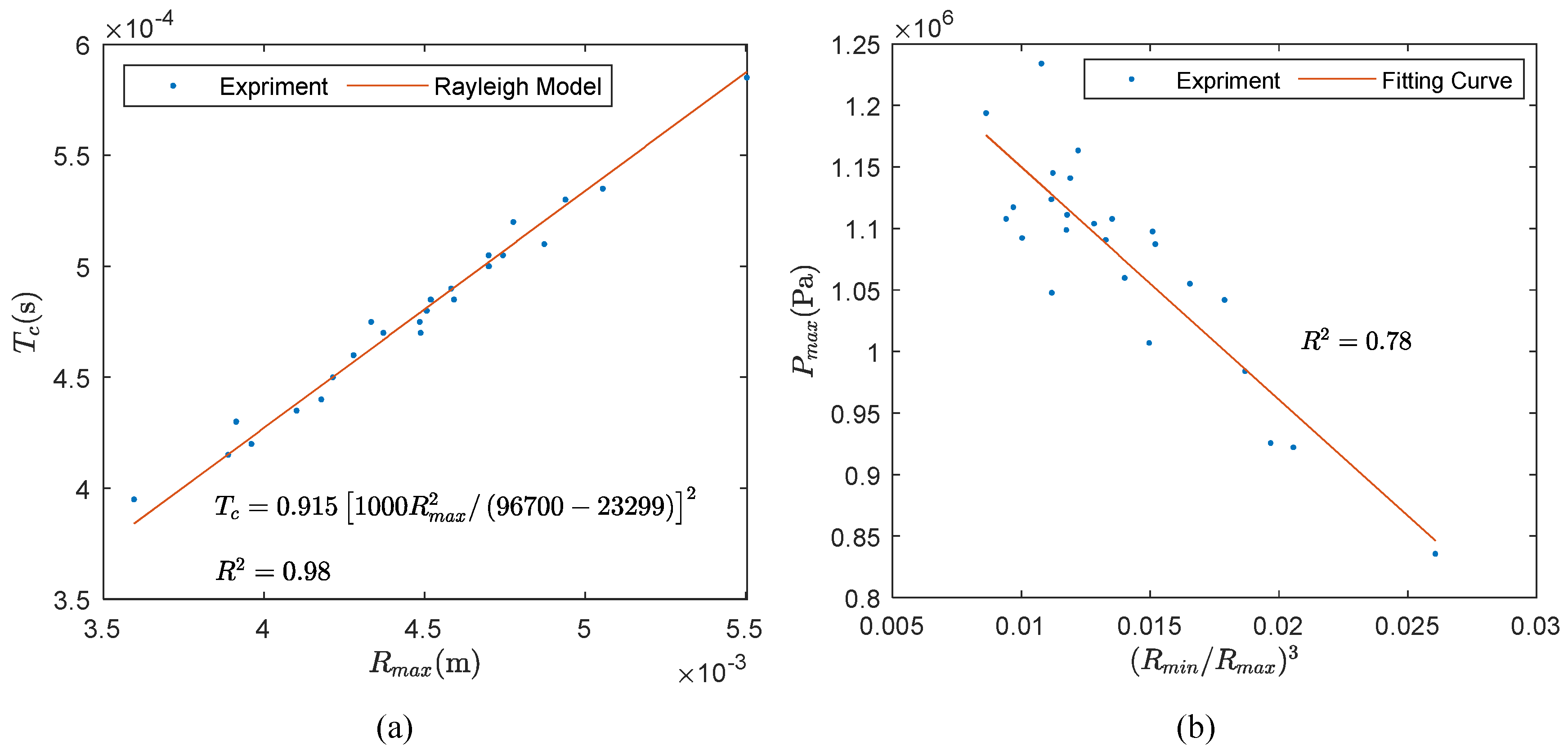
4.2. Statistical Properties
5. Conclusions
Author Contributions
Funding
Conflicts of Interest
References
- Harrison, M. An Experimental Study of Single Bubble Cavitation Noise. J. Acoust. Soc. Am. 1952, 24, 776–782. [Google Scholar] [CrossRef]
- Shutler, N.D.; Mesler, R.B. A Photographic Study of the Dynamics and Damage Capabilities of Bubbles Collapsing Near Solid Boundaries. J. Basic Eng. 1965, 87, 511–517. [Google Scholar] [CrossRef]
- Shima, A.; Takayama, K.; Tomita, Y.; Ohsawa, N. Mechanism of impact pressure generation from spark-generated bubble collapse near a wall. AIAA J. 1983, 21, 55–59. [Google Scholar] [CrossRef]
- Ward, B.; Emmony, D.C. Direct observation of the pressure developed in a liquid during cavitation-bubble collapse. Appl. Phys. Lett. 1991, 59, 2228–2230. [Google Scholar] [CrossRef]
- Luo, J.; Xu, W.; Deng, J.; Zhai, Y.; Zhang, Q.; Luo, J.; Xu, W.; Deng, J.; Zhai, Y.; Zhang, Q. Experimental Study on the Impact Characteristics of Cavitation Bubble Collapse on a Wall. Water 2018, 10, 1262. [Google Scholar] [CrossRef]
- Jayaprakash, A.; Hsiao, C.-T.; Chahine, G. Numerical and Experimental Study of the Interaction of a Spark-Generated Bubble and a Vertical Wall. J. Fluids Eng. 2012, 134, 031301. [Google Scholar] [CrossRef]
- Ma, X.; Huang, B.; Zhao, X.; Wang, Y.; Chang, Q.; Qiu, S.; Fu, X.; Wang, G. Comparisons of spark-charge bubble dynamics near the elastic and rigid boundaries. Ultrason. Sonochem. 2018, 43, 80–90. [Google Scholar] [CrossRef] [PubMed]
- Lauterborn, W.; Bolle, H. Experimental investigations of cavitation-bubble collapse in the neighbourhood of a solid boundary. J. Fluid Mech. 1975, 72, 391–399. [Google Scholar] [CrossRef]
- Philipp, A.; Lauterborn, W. Cavitation erosion by single laser-produced bubbles. J. Fluid Mech. 1998, 361, 75–116. [Google Scholar] [CrossRef]
- Lim, K.Y.; Quinto-Su, P.A.; Klaseboer, E.; Khoo, B.C.; Venugopalan, V.; Ohl, C.-D.D. Nonspherical laser-induced cavitation bubbles. Phys. Rev. E Stat. Nonlinear Soft Matter Phys. 2010, 81, 016308. [Google Scholar] [CrossRef] [PubMed]
- Vogel, A.; Brujan, E.A.; Schmidt, P.; Nahen, K. Interaction of laser-produced Cavitation bubbles with elastic boundaries. In IUTAM Symposium on Free Surface Flows; Fluid Mechanics and Its Applications; Springer: Dordrecht, The Netherlands, 2001; Volume 62, pp. 327–335. [Google Scholar]
- Tomita, Y.; Kodama, T. Interaction of laser-induced cavitation bubbles with composite surfaces. J. Appl. Phys. 2003, 94, 2809–2816. [Google Scholar] [CrossRef]
- Philipp, A.; Lauterborn, W. Damage of Solid Surfaces by Single Laser-Produced Cavitation Bubbles. Acta Acust. United Acust. 1997, 83, 223–227. [Google Scholar]
- Han, B.; Liu, L.; Zhao, X.-T.; Ni, X.-W. Liquid jet formation through the interactions of a laser-induced bubble and a gas bubble. AIP Adv. 2017, 7, 105305. [Google Scholar] [CrossRef]
- Lindau, O.; Lauterborn, W. Cinematographic observation of the collapse and rebound of a laser-produced cavitation bubble near a wall. J. Fluid Mech. 2003, 479, 327–348. [Google Scholar] [CrossRef]
- Vogel, A.; Lauterborn, W. Acoustic transient generation by laser-produced cavitation bubbles near solid boundaries. J. Acoust. Soc. Am. 1988, 84, 719–731. [Google Scholar] [CrossRef]
- Hentschel, W.; Lauterborn, W. Acoustic emission of single laser-produced cavitation bubbles and their dynamics. Appl. Sci. Res. 1982, 38, 225–230. [Google Scholar] [CrossRef]
- Sato, T.; Tinguely, M.; Oizumi, M.; Farhat, M. Evidence for hydrogen generation in laser- or spark-induced cavitation bubbles. Appl. Phys. Lett. 2013, 102, 074105. [Google Scholar] [CrossRef]
- Fong, S.W.; Adhikari, D.; Klaseboer, E.; Khoo, B.C. Interactions of multiple spark-generated bubbles with phase differences. Exp. Fluids 2009, 46, 705–724. [Google Scholar] [CrossRef]
- Luo, J.; Xu, W.; Li, R. High-speed photographic observation of collapse of two cavitation bubbles. Sci. China Technol. Sci. 2016, 59, 1707–1716. [Google Scholar] [CrossRef]
- Xu, W.; Zhang, Y.; Luo, J.; Zhang, Q.; Zhai, Y. The impact of particles on the collapse characteristics of cavitation bubbles. Ocean Eng. 2017, 131, 15–24. [Google Scholar] [CrossRef]
- Poulain, S.; Guenoun, G.; Gart, S.; Crowe, W.; Jung, S. Particle motion induced by bubble cavitation. Phys. Rev. Lett. 2015, 114. [Google Scholar] [CrossRef] [PubMed]
- Ohl, S.-W.; Wu, D.W.; Klaseboer, E.; Khoo, B.C. Spark bubble interaction with a suspended particle. J. Phys. Conf. Ser. 2015, 656, 012033. [Google Scholar] [CrossRef]
- Li, S.; Zhang, A.M.; Wang, S.; Han, R. Transient interaction between a particle and an attached bubble with an application to cavitation in silt-laden flow. Phys. Fluids 2018, 30, 082111. [Google Scholar] [CrossRef]
- Zhang, A.M.; Cui, P.; Wang, Y. Experiments on bubble dynamics between a free surface and a rigid wall. Exp. Fluids 2013, 54, 1602. [Google Scholar] [CrossRef]
- Cui, P.; Zhang, A.M.; Wang, S.P. Small-charge underwater explosion bubble experiments under various boundary conditions. Phys. Fluids 2016, 28, 117103. [Google Scholar] [CrossRef]
- Zhang, S.; Wang, S.; Zhang, A.M. Experimental study on the interaction between bubble and free surface using a high-voltage spark generator. Phys. Fluids 2016, 28, 032109. [Google Scholar] [CrossRef]
- Longuet-Higgins, M.S. Bubbles, breaking waves and hyperbolic jets at a free surface. J. Fluid Mech. 1983, 127, 103–121. [Google Scholar] [CrossRef]
- Luo, J.; Xu, W.; Niu, Z.; Luo, S.; Zheng, Q. Experimental study of the interaction between the spark-induced cavitation bubble and the air bubble. J. Hydrodyn. Ser. B 2013, 25, 895–902. [Google Scholar] [CrossRef]
- Xu, W.; Bai, L.; Zhang, F. Interaction of a cavitation bubble and an air bubble with a rigid boundary. J. Hydrodyn. 2010, 22, 503–512. [Google Scholar] [CrossRef]
- Kannan, Y.S.; Karri, B.; Sahu, K.C. Letter: Entrapment and interaction of an air bubble with an oscillating cavitation bubble. Phys. Fluids 2018, 30, 041701. [Google Scholar] [CrossRef]
- Goh, B.H.T.; Oh, Y.D.A.; Klaseboer, E.; Ohl, S.W.; Khoo, B.C. A low-voltage spark-discharge method for generation of consistent oscillating bubbles. Rev. Sci. Instrum. 2013, 84. [Google Scholar] [CrossRef] [PubMed]
- Bradley, D.G.R. Adapting Thresholding Using the Integral Image. J. Gr. Tools 2018, 12, 13–21. [Google Scholar] [CrossRef]


| Day Average Temperature (°C) | Atmospheric Pressure (kPa) | Humidity (%) |
|---|---|---|
| 5.6 | 96.7 | 93 |
| −9.4 × 10⁻⁶ | 1.1 × 10⁻⁵ | −1.1 × 10⁻² | 5.8 × 10⁻⁴ | 9.0 × 101 | |
| −5.9 × 10⁻⁵ | −2.0 × 10⁻⁴ | −2.0 × 10⁻² | −5.0 × 10⁻² | 5.9 × 101 |
© 2018 by the authors. Licensee MDPI, Basel, Switzerland. This article is an open access article distributed under the terms and conditions of the Creative Commons Attribution (CC BY) license (http://creativecommons.org/licenses/by/4.0/).
Share and Cite
Zhang, Q.; Luo, J.; Zhai, Y.; Li, Y. Improved Instruments and Methods for the Photographic Study of Spark-Induced Cavitation Bubbles. Water 2018, 10, 1683. https://doi.org/10.3390/w10111683
Zhang Q, Luo J, Zhai Y, Li Y. Improved Instruments and Methods for the Photographic Study of Spark-Induced Cavitation Bubbles. Water. 2018; 10(11):1683. https://doi.org/10.3390/w10111683
Chicago/Turabian StyleZhang, Qi, Jing Luo, Yanwei Zhai, and Yilan Li. 2018. "Improved Instruments and Methods for the Photographic Study of Spark-Induced Cavitation Bubbles" Water 10, no. 11: 1683. https://doi.org/10.3390/w10111683
APA StyleZhang, Q., Luo, J., Zhai, Y., & Li, Y. (2018). Improved Instruments and Methods for the Photographic Study of Spark-Induced Cavitation Bubbles. Water, 10(11), 1683. https://doi.org/10.3390/w10111683