Article

Predicting Taste and Odor Compounds in a Shallow Reservoir Using a Three–Dimensional Hydrodynamic Ecological Model

1
K-water Convergence Institute, Korea Water Resources Corporation (K-water), Daejeon 34045, Korea
2
Department of Biological Science, College of Biological Sciences and Biotechnology, Chungnam National University, Daejeon 34134, Korea
*
Author to whom correspondence should be addressed.
Water 2018, 10(10), 1396; https://doi.org/10.3390/w10101396
Submission received: 12 September 2018 / Revised: 1 October 2018 / Accepted: 4 October 2018 / Published: 9 October 2018
(This article belongs to the Special Issue Freshwater Quality as a Driver of Aquatic Ecosystem Health)

Abstract

:
The objective of this study was to establish a technique to predict the occurrence of algal bloom and the algal-derived taste and odor compounds 2-methylisoborneol (2-MIB) and geosmin using a three-dimensional (3D) model that could reflect the complex physical properties of a shallow reservoir. Water quality, phytoplankton, and taste and odor compounds monitoring was conducted at the Jinyang Reservoir in 2016. In June, there was a potential for a high concentration of 2-MIB (maximum 80 ng/L) to occur owing to the appearance of Pseudanabaena sp.; additionally, from July to August, there was potential for a high concentration of geosmin (maximum 108 ng/L) to occur, because of the presence of Anabaena sp. A 3D hydrodynamic model was coupled with an ecological model to predict cyanobacteria bloom and the presence of taste and odor compounds. Cyanobacteria producing either 2-MIB or geosmin were distinguished to enhance the accuracy of the modeled predictions. The results showed that the simulations of taste and odor compounds spatial distribution and occurrence time were realistic; however, the concentration of geosmin was overestimated when Microcystis sp. was blooming. The model can be used as a management tool to predict the occurrence of algal taste and odor compounds in reservoir systems and to inform decision-making processes concerning dam operation and water treatment.

1. Introduction

Harmful algal blooms (HABs) are a major environmental problem that tends to occur more frequently than previously worldwide, causing ecological, aesthetic, and health problems [1,2,3]. In particular, cyanobacteria blooms may cause serious problems for drinking water supplies by producing metabolites like toxins and taste and odor compounds or by clogging sand filters during the water treatment process. 2-methylisoborneol (2-MIB) and trans-1,10-dimethyl-trans-9-decalol (geosmin) are representative substances causing earthy/musty/moldy taste and odor, and thus, have attracted researchers’ attention [4,5]. Since these compounds can be detected by human noses at very low levels (10 ng/L or below), it is very difficult to predict their occurrence. Moreover, these compounds are difficult to remove by conventional water treatment processes; they can be removed only by advanced treatment processes using oxidation with ozone or activated carbon adsorption, which come at high financial cost [6,7].
Many studies have dealt with major cyanobacteria that produce geosmin and 2-MIB. Numerous researchers have showed that Anabaena sp. produces geosmin. Aphanizomenon sp. has been recognized as belonging to a cyanobacteria genus that produces geosmin [8,9,10,11,12,13]. It has been reported that Oscillatoria sp. and Phormidium sp. produce both geosmin and 2-MIB, depending on the species [8,9,10,11,12,13]. Pseudanabaena sp. generates mainly 2-MIB, while Microcystis sp., which is one of the most frequently discovered cyanobacteria blooms, produces neither geosmin, nor 2-MIB [8,9,10,11,12,13]. However, Zhang et al. [14] reported that although it is not frequent, Microcystis aeruginosa did sometimes produce 2-MIB. In recent years, studies on cyanobacteria producing taste and odor compounds have been actively carried out using molecular biology methods [15,16,17,18]. The concentrations of geosmin and 2-MIB, which are generated by the metabolism of cyanobacteria, are known to naturally decrease through mechanisms such as volatilization, photolysis, sorption, and biodegradation [19]. However, if they are present in drinking water without being treated, a serious problem may occur. Accordingly, the importance of predicting algal blooms and the resulting geosmin and 2-MIB has been continuously reinforced. Over the last decade, many modeling studies have been attempted to predict taste and odor compounds. Dzialowski et al. [20] developed an empirical regression model to predict geosmin in five drinking water reservoirs in Kansas, USA. Bradley [21] also developed a similar empirical model using a multiple logistic regression model in order to predict geosmin concentrations in Lake Bowen. In Canada, Parinet, Rodriguez, and Sérodes [22] attempted to predict geosmin concentrations of raw water supplied to Quebec City by developing a prediction model through multi-linear regression, principal component regression, and evaluating multi-layer perceptrons. Bruder [23] tried to combine a numerical model and a heuristic model to predict concentrations of geosmin and 2-MIB in the Eagle Creek reservoir. They utilized the adaptive network-based fuzzy inference system (ANFIS) and the environmental fluid dynamics code (EFDC). Recently, Harris and Graham [24] developed linear and nonlinear regression models to predict cyanobacterial abundance and the presence of the cyanobacterial secondary metabolites microcystin and geosmin, using long-term physiochemical water quality data collected from the Cheney Reservoir. Most models developed in previous studies have been empirical and were applicable only to specific water bodies. They cannot comprehensively analyze complex factors such as weather, hydraulic features, water quality, and ecological processes in a reservoir. Many other recent studies have used a numerical model to reflect physical, physiological, and ecological processes, and were able predict the occurrence of cyanobacteria [25,26,27,28]. However, few studies have attempted to predict taste and odor compounds that are metabolites of cyanobacteria. Islam et al. [29] have developed a numerical model to predict toxins produced by Microcystis blooms in Lake Kasumigaura, Japan. The results revealed that light intensity, temperature, water depth, wind direction, buoyancy, and nitrogen:phosphorus (N:P) ratio are the factors that affect toxin production. Chung et al. [30] have developed a predictive model for geosmin in the North Han River, Korea, based on a two-dimensional hydrodynamic and mass transport model (CE-QUAL-W2). They successfully captured the outbreaks of geosmin produced by Anabaena sp. These mechanistic water quality models can dynamically predict spatially variable metabolites; however, they need substantial amounts of valid data or there could be large deviations between the real-world and simulated situations, depending on the assumptions used.
This study attempts to quantitatively predict taste and odor compounds occurring during the growth and extinction of cyanobacteria by using three-dimensional hydrodynamic ecological models. Spatial and temporal occurrences of algae and algal-derived taste and odor compounds are dynamically modeled by coupling the estuary, lake, and coastal ocean model (ELCOM), which can reflect complex physical features of a man-made reservoir, with the computational aquatic ecosystem dynamic model (CAEDYM), which reproduces ecological properties of algae very well. The study site was the Jinyang Reservoir (Namgang Dam) in South Korea, which is a large water supply source and a shallow reservoir showing very dynamic physical properties. It was reported that a cyanobacteria bloom with geosmin and 2-MIB occurred between 2014 and 2016 at the site. This study predicts the concentrations of algae and taste and odor compounds to inform decision-making processes concerning dam operation and water treatment.

2. Materials and Methods

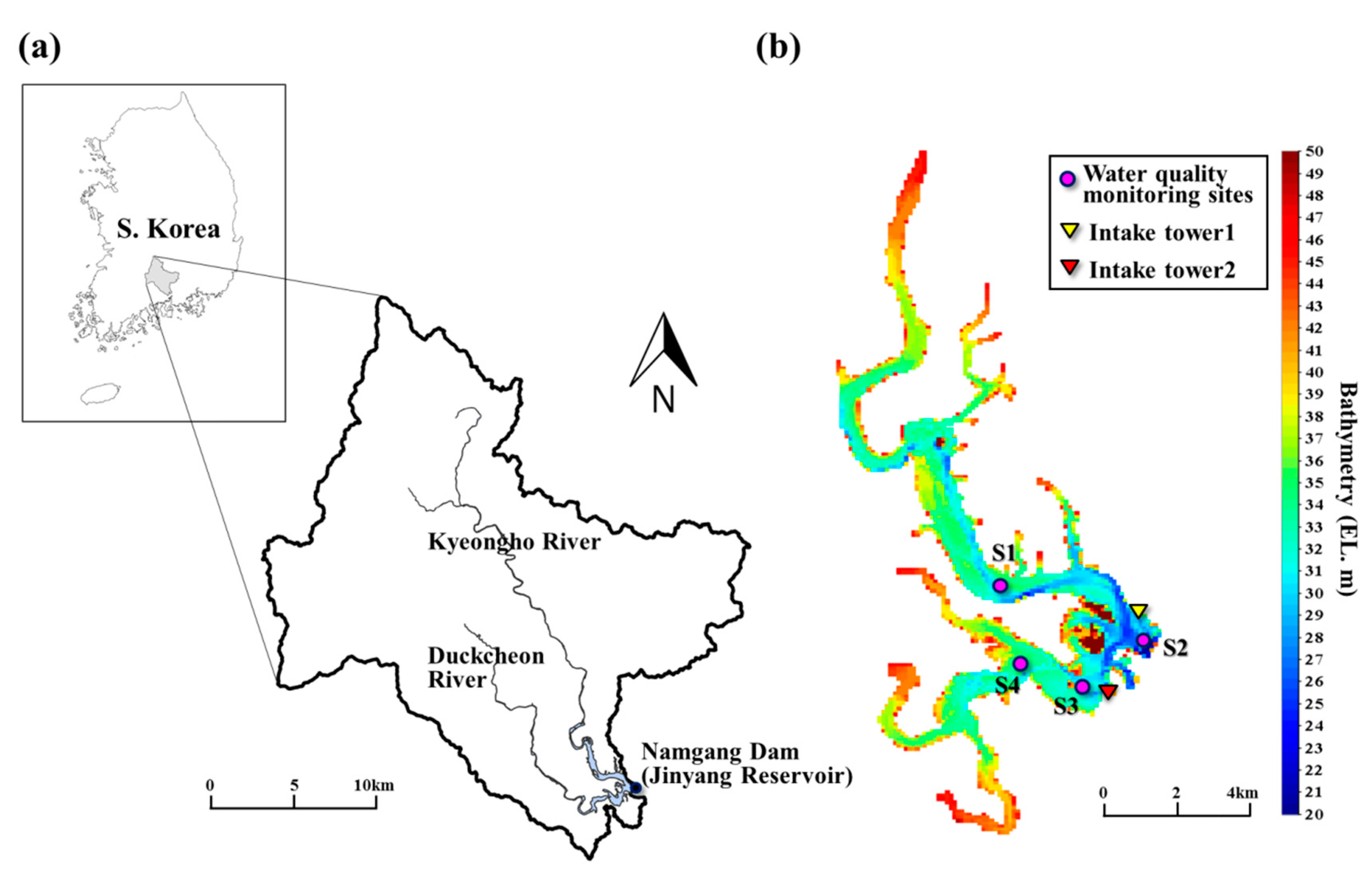
2.1. Description of the Study Site

The Namgang Dam is a multipurpose dam for flood control, water supply, etc., located in the Nam River (35°15′ N, 128°23′ E), which is a tributary of the Nakdong River. The man-made reservoir formed by the construction of Namgang Dam is called the Jinyang Reservoir. The reservoir’s catchment area is 2293 km2, its storage capacity is 309.2 × 10⁶ m3, and its maximum water depth is 20 m. This reservoir is a typical shallow reservoir with an average water depth of 7.5 m and an average annual retention time of 25 days. The Kyeongho River and Duckcheon River are the main inflow streams (Figure 1a). The catchment area of the Kyeongho River is 1773.2 km2, which is about five times larger than the 354.6 km2 of the Duckcheon River. The Jinyang Reservoir is a very important water intake source for the southwestern part of Gyeongsangnam-do. Drinking water produced using the Namgang Dam as the water intake source is provided to 820,000 people in seven district regions (Si and Gu). As for the quantity of water intake in the Namgang Dam, the Namgang Intake Station (Intake tower 2), located in the area of Duckcheon River inflow, has the largest capacity of 261,000 m3/day, followed by 220,000 m3/day for the Jinju Intake Station (Intake tower 1) located in the area of Kyeongho River inflow (Figure 1b).

2.2. Analysis of Water Quality, Phytoplankton and Taste and Odor Compounds

To analyze the characteristics of algae and taste and odor compounds occurring in the Jinyang Reservoir, this study conducted a field survey from April to November 2016. Water quality and algae were monitored biweekly from June to August, when algae frequently occurred, while other items were surveyed monthly. Water quality was monitored at four sites: the Kyeongho River zone (S1), the front of the dam (S2), the Namgang wide-area water supply intake tower (S3), and the Duckcheon River zone (S4) (Figure 1b). Water samples were collected from upper, middle, and lower layers at each site and were analyzed. A water quality measurement instrument (Troll 9500 from In-Situ, Fort Collins, CO, USA) was used to measure water temperature, dissolved oxygen (DO), pH, conductivity, and turbidity during sampling. Sterilized water sample bottles were used to carry water samples to the laboratory, where water quality items like organic matter and nutrients were analyzed and physicochemical causes of algae and taste and odor compounds were comparatively analyzed.
Chlorophyll-a (Chl-a), phosphate (PO4-P), nitrate (NO3-N), ammonium (NH4-N), total phosphorus (TP), and total nitrogen (TN) were analyzed based on the standard methods [31]. The number of cyanobacterial cells was immediately fixed by using Lugol’s solution (Lugol:formalin = 3:1 (v/v)) and was concentrated by 24-h settlement. After the cells were counted using a Sedgwick-Rafter chamber, the numbers were marked per mL. Geosmin and 2-MIB, which have been recognized as causes of taste and odor compounds, were measured by applying the solid-phase micro-extraction (SPME) gas chromatography mass spectrophotometry (GC/MS) method and using GC (450 GC)/MS (300 MS) (Bruker). Samples were collected every 10 mL and put into vials. Then sodium chloride was added and the samples were analyzed using GC/MS. For quantitative analysis, 112 m/z ions of geosmin and 95 m/z ions of 2-MIB were selected and evaluated.
Moreover, in order to analyze the physical causes of algal bloom and taste and odor compounds at the Namgang Dam, hydrological and meteorological data were collected and relevant properties were analyzed for the study period. Changes in precipitation patterns and air temperature can affect the timing, duration, and intensity of the cyanobacteria bloom and the production of taste and odor compounds. Therefore, we attempted to analyze the physical factors affecting the occurrence of cyanobacteria by comparing historical monthly weather data and that from the study period. Daily operation data of the water resources information system (WRIS) for K-water were used as the hydrological data. For the meteorological data, rainfall, and temperature data from the Jinju Observatory of the Korea Meteorological Administration (KMA) were collected and compared with average measurements over 30 years (1981–2010) [32].

2.3. Model Description

The estuary, lake, and coastal ocean model (ELCOM) is a three-dimensional hydrodynamic model that can be applied to lakes, reservoirs, estuaries, and oceans. ELCOM was developed by the Center for Water Research (CWR) of the University of Western Australia. Coupled with the computational aquatic ecosystem dynamic model (CAEDYM), ELCOM provides three-dimensional numerical analysis results for dynamic modeling of the water quality and ecosystem of a lake or reservoir. The governing equations include momentum equations, a continuity equation, a free-surface equation, and a transfer–diffusion equation. Reynolds-averaged Navier–Stokes (RANS) equations were used. The Boussinesq assumption was applied to apply the characteristics of the fluid and the hydrostatic pressure theory was used for the vertical momentum equation. However, in case the non-hydrostatic pressures are important, a non-hydrostatic code can be used to include a vertical momentum equation [33].
Momentum equation:
x-momentum:
u t + u u x + v u y + w u z = g { η x + 1 ρ 0 x z η ρ d z } + x { v h u x } + y { v h u y } + z { v h u z } + f v
y-momentum:
v t + u v x + v v y + w v z =        g { η y + 1 ρ 0 y z η ρ d z } + x { v h v x } + y { v h v y } + z { v v v z }        f u
z-momentum (hydrostatic pressure assumption):
p z = ρ g
Continuity:
u x + v y + w z = 0
Free surface evolution:
η t + x [ h 0 η u d z ] + y [ h 0 η v d z ] = 0
Transport of scalars:
c t + u c x + v c y + w c z = x { k h c x } + y { k h c y } + z { k v c z } + S c
where u is x-direction velocity (m/s), v is y-direction velocity (m/s), w is z-direction velocity (m/s), g is gravitational acceleration (9.81 m/s2), η is Reynolds-averaged free-surface height (m), ρ is density (kg/m3), ρ 0 is the reference density (kg/m3), ρ is the density anomaly (kg/m3), v h is turbulent eddy viscosity (m2/s), p is pressure (N/m2), f is the Coriolis constant (2 ωsinφ, ω is angular velocity of the earth around its axis, 7.29 × 10⁻⁵ rad/s, and φ is latitude), k v is vertical eddy viscosity (m2/s), and k h is horizontal eddy viscosity (m2/s).
CAEDYM is an aquatic ecosystem model designed to be coupled with various numerical models. One of the remarkable advantages of CAEDYM is that cycles of diverse materials and various algal groups in an aquatic ecosystem can be modeled. In other words, this model can cover both water quality modeling items like various cycles of C, N, P, and Si, the DO cycle, inorganic suspended substances (SS), and ecological modeling items like phytoplankton, zooplankton, and fish. As CAEDYM can simulate seven groups of phytoplankton, it can accurately reproduce the characteristics of algae according to environmental factors. Furthermore, this model can also simulate representative algal-derived taste and odor compounds. In this respect, it seemed very suitable for this study. The governing equation for calculating algal-derived metabolites (Xa, mg/L) is as follows [34]:
X a t = f A a B M E f X a M I N
where f A a B M E is the metabolite contribution from mortality and excretion by Aa and f X a M I N is the bacterially mediated decay of metabolites defined as:
f A a B M E = I X a A a ( 1 f R E S a ) L a f ( S ) a
f X a M I N = m x X a
where I X a is the internal metabolite concentration of A a ( m g / L m g C h l a / L ), A a is the biomass of the ath phytoplankton group in chlorophyll-a units ( m g C h l a / L ), f R E S a represents the isolated true respiration losses from the lumped parameterization (including respiration, natural mortality, and excretion), f ( S ) a is a loss term multiplier used as the respiration response to salinity, and m x is a degradation rate constant for X a (/d). The metabolite concentration within the algal cells, I X a , is considered to be a linear function of the growth rate:
I X a = I X a M I N + μ g a μ M A X a ( I X a M A X I X a M I N )
where I X a M I N is the minimum internal metabolite (i.e., when the growth rate is zero) and I X a M A X is the internal metabolite concentration during maximum production.

2.4. Configuration and Application of the Model

Figure 1b shows a bathymetry map of the ELCOM model applied to the Namgang Dam, which was the study site. The size of each grid cell was 100 × 100 × 1 m (Δx × Δy × Δz) and the total well cells constituted 55,010 grids. The boundary conditions of tributary inflow included the Kyeongho River and Duckcheon River. The boundary conditions of outflow were divided into gate outflow, hydropower outflow, the Jinju intake tower, and the Namgang wide area water supply intake tower. The inflow and outflow of each site were based on the daily data of the WRIS for K-water. For meteorological data, hourly data for temperature, relative humidity, wind direction, wind speed, atmospheric pressure, solar radiation, and cloud cover were provided from the Jinju Observatory of the KMA. For the boundary water quality concentration, 14 constituents were input, including water temperature, dissolved organic carbon (DOC), particulate organic carbon (POC), dissolved organic nitrogen (DON), particulate organic nitrogen (PON), dissolved organic phosphorus (DOP), particulate organic phosphorus (POP), dissolved oxygen (DO), inorganic nutrients (NO3-N, NH4-N, PO4-P), cyanobacteria 1 (causing 2-MIB), cyanobacteria 2 (causing geosmin), and freshwater diatoms. Moreover, TN, TP, and metabolites (2-MIB and geosmin) were additional outputs for modeling. The modeling period was eight months from April to November, 2016. The calculation interval was 60 s.

2.5. Assessment of Model Performance

Model performance was assessed using the root-mean-square error (RMSE) and the absolute mean error (AME). These statistics are frequently used to examine the goodness of fit between modeling results and observed values. They are calculated by the following equations:
RMSE = i = 1 n ( O i P i ) 2 n
AME = i = 1 n | O i P i | n
where n is the number of measured and predicted pairs, O is an observed value, and P is a predicted value. Model performance evaluation were performed for various water quality parameters, DO, nitrate, total organic carbon (TOC), TP, and Chl-a. Finally, we evaluated the fit of the model for taste and odor compounds, 2-MIB, and geosmin.

3. Results of the Field Survey for Algae and Taste and Odor Compounds

3.1. Meteorological and Hydrological Properties

In 2016, the deviation of monthly rainfall was much larger than the climatological normal (over 30 years from 1980 to 2010). From February to April and from September to October, the rainfall amount was larger than the climatological normal, while during the summer season, from June to August, it was far less than the climatological normal (Table 1). In particular, the rainfall during August was only 24% of the climatological normal; this was a very unusual pattern. Accordingly, the monthly average inflow was 27.6% in June and 8.5% in August, as compared to the 40-year average value after the construction of the dam. As for temperature, the annual average temperature was 0.7 °C higher than the average. In particular, the average temperature during August was 1.0 °C higher than the climatological normal, which reflected excessively hot weather during that period. Due to such low rainfall, the meteorological and hydrological data for the Namgang Dam in 2016 show a small amount of inflow and outflow. Consequently, as the water body was stable and high water temperatures continued, algae were more likely to grow.

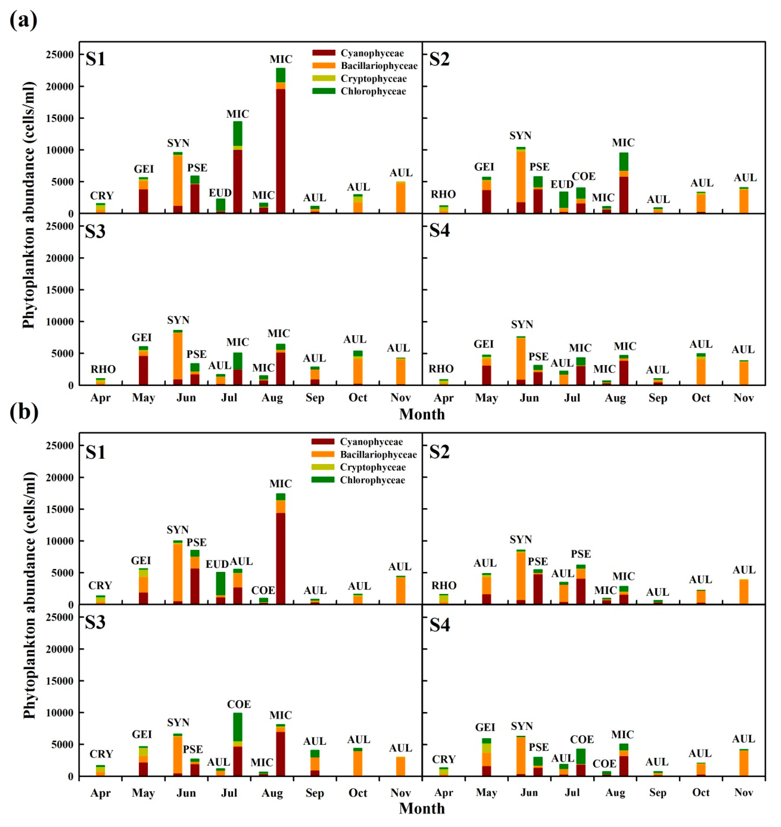
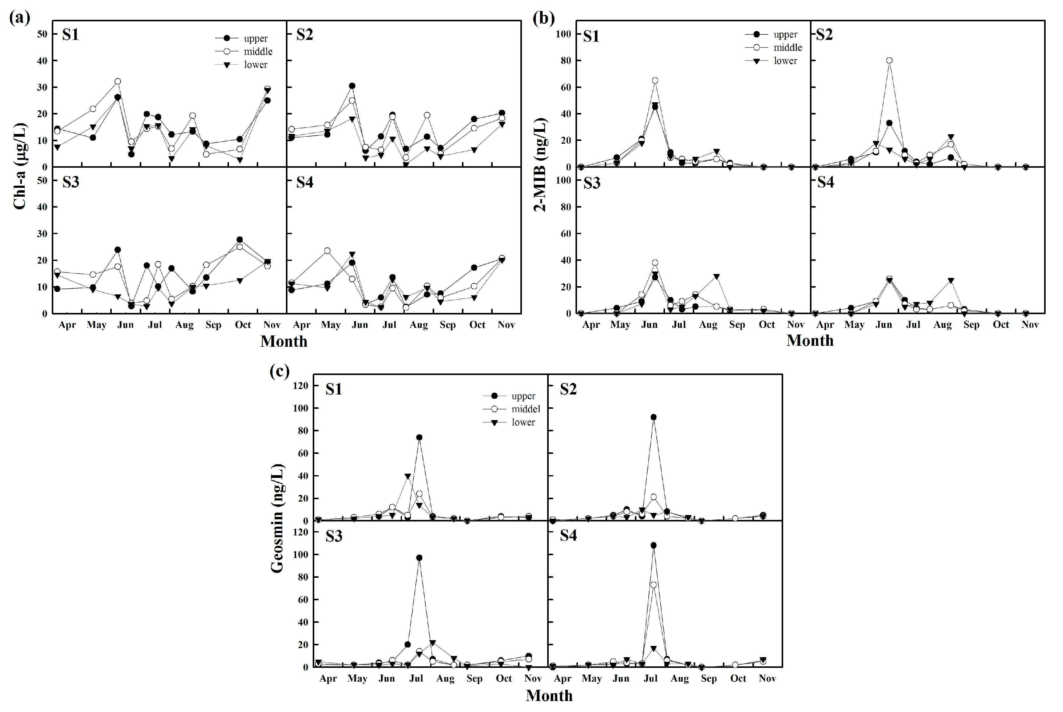
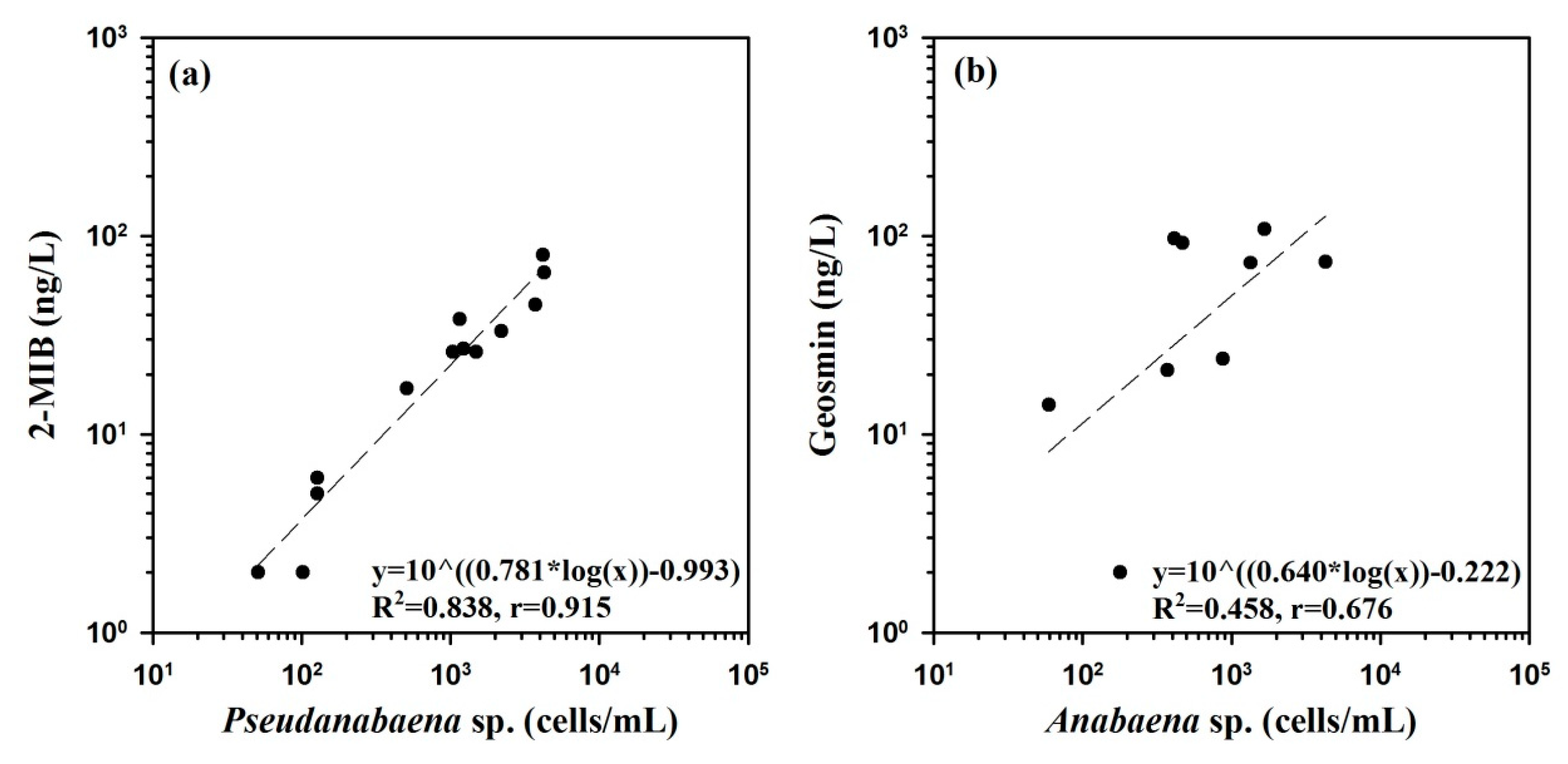
3.2. Characteristics of Algae and Taste and Odor Compound Occurrence

Total algal population observed during the study period was in the range of 646–22,845 cells/mL and the average population was 4475 cells/mL. There were large deviations depending on seasons and sites (Figure 2). The largest average algal population of 6137 cells/mL (in the range of 867–22,845 cells/mL) was observed at S1, while S4 showed the smallest average population of 3374 cells/mL in the range of 729–7649 cells/mL. In 2016, the algal population showed an overall increasing tendency with the dominance of Synedra sp. and Pseudanabaena sp. in June and Microcystis sp. and Anabaena sp. from July to August. In June, when the algal population showed its highest increase, owing to low rainfall, Synedra sp. and Pseudanabaena sp. were dominant, clogging sand filters and, potentially causing a high concentration of 2-MIB. In August, the dominance of Microcystis sp. and Anabaena sp. led to an increase in harmful cyanobacteria, resulting in frequent algal bloom alerts and potentially high concentrations of geosmin. Synedra sp., which clogged sand filters, was most frequently observed in the middle layer of S1 during the study period. The population of Synedra sp. was 8202 cells/mL. As the population of Synedra sp. decreased, that of Pseudanabaena sp. quickly increased, generating 2-MIB. The largest population of Pseudanabaena sp. was 4257 cells/mL in the middle layer of S1. Microcystis sp. had the largest population of 14,484 cells/mL in the upper layer of S1. The population of Anabaena sp., which produced geosmin, was as large as 4278 cells/mL in the middle of July in the upper layer of S1.
During the survey, the average concentration of chlorophyll-a in the Namgang Dam was 12.4 mg/m3 in the range of 1.0–32.1 mg/m3. There was a slight deviation depending on the season and site, but no significant relevance to algal population was found (Figure 3a). The average concentration of chlorophyll-a at S1 was 14.6 mg/m3 (in the range of 2.9–32.1 mg/m3); that at S2 was 12.1 mg/m3 (in the range of 1.0–30.5 mg/m3); that at S3 was 12.5 mg/m3 (in the range of 2.7–27.7 mg/m3); and that at S4 was 10.3 mg/m3 (in the range of 2.2–23.5 mg/m3). S1 showed the highest average concentration, while S4 showed the lowest.
The concentrations of algal-derived taste and odor compounds (2-MIB and geosmin) showed large deviations depending on the season and site. 2-MIB showed the highest concentration of 80 ng/L in the middle layer at S2, and the highest concentration of geosmin was 108 ng/L, which was observed in the upper layer at S4 (Figure 3b). In other words, 2-MIB had high concentrations in the middle layers in June, while geosmin had the highest concentration in the upper layer in July (Figure 3c). Generally, geosmin and 2-MIB increased with cyanobacteria (Figure 4). When the concentration of 2-MIB was observed to be as high as 80 ng/L between middle to late June, Pseudanabaena sp. was the dominant cyanobacteria and was identified as the potential cause (Figure 4a). The highest concentration of geosmin was 108 ng/L; at that time, the dominant species was Microcystis sp., however, the potential cause of taste and odor compounds seemed to be Anabaena sp., which was the subdominant species (Figure 4b).

4. Model Prediction Results for Algae and Taste and Odor Compounds

4.1. Model Validation

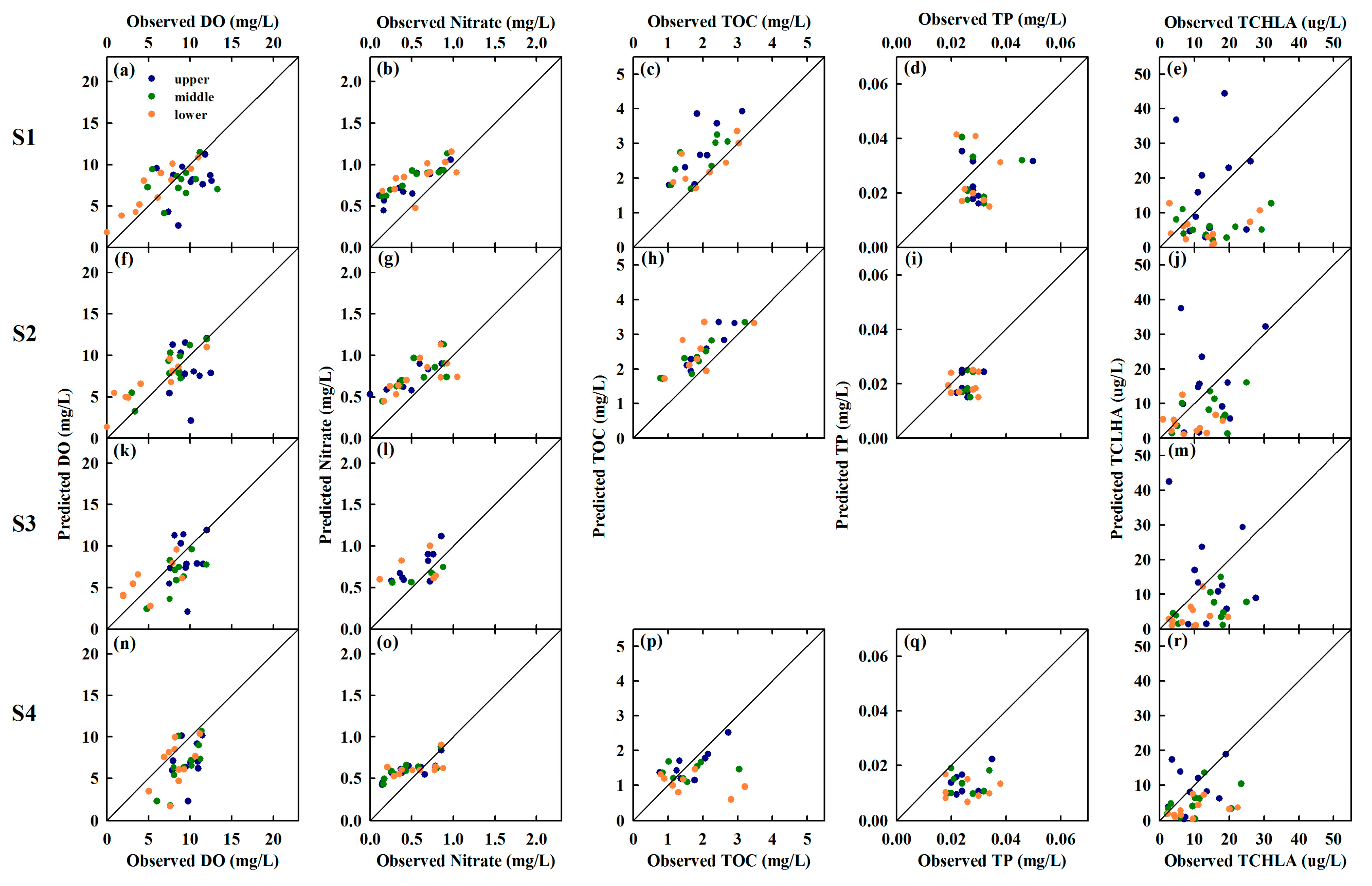
4.1.1. Water Quality

Table 2 and Table 3 present hydraulic and water quality parameters, respectively, along with values applied in the previous studies. Most of the hydraulic and water quality parameters had a similar range of inputs to those of previous studies. CAEDYM can basically model cyanobacteria group 1. However, to distinguish cyanobacteria causing 2-MIB and geosmin in the results of the field survey, this study used CAEDYM to simulate two cyanobacteria groups (CYANO1 and CYANO2). Table 3 shows the parameters used for calibrating the model. This study distinguished CYANO1 and CYANO2. CYANO1 represents Pseudanabaena sp. causing 2-MIB in water while, for CYANO2, Anabaena sp. is the representative species causing geosmin. Other dominant diatoms were modeled as a single group (FDAIT). The major parameters for modeling different cyanobacteria groups were optimum temperature (Topt) and maximum temperature (Tmax). CYANO1 causing 2-MIB was modeled to optimally grow in a lower temperature range than CYANO2. However, according to many field surveys and experimental culture studies, a very wide range of water temperatures affect the growth of Anabana sp. [35,36,37,38,39] and Psedanabana sp. [40,41,42,43,44]. Therefore, the applied optimal and maximum temperatures are limited to this study, and it is necessary to improve the model validation by obtaining additional data.
The results of the water quality model calibration are presented by comparing DO, NO3-N, TOC, TP, and chlorophyll-a between model estimates and measurements (Figure 5). Most of the evaluation constituents show that the model accurately reproduced the seasonal change of water quality and the spatial distribution of water quality and algal concentrations. The results of DO modeling revealed that the model reproduced very accurately the hypoxic phenomenon, indicating a DO level of 5 mg/L or less, which was observed in the bottom layers of S1–S3. The RMSE for the DO value was 2.5–3.4 mg/L and the AME was 1.9–2.8 mg/L. For NO3-N, TOC, and TP, there was not a significant difference in concentration (Table 4). S4 showed a smaller model error than at other points. The calibration results of chlorophyll-a accurately reproduced the high concentrations in the surface layer in terms of water quality and also provided good reproduction of the spatial characteristics, i.e., that S1 had the greatest algal biomass, while S4 showed the smallest. The RMSE and AME of chlorophyll-a were assessed to be 8.5–13.4 μg/L and 6.3–10.6 μg/L, respectively, both quantities within the error range.

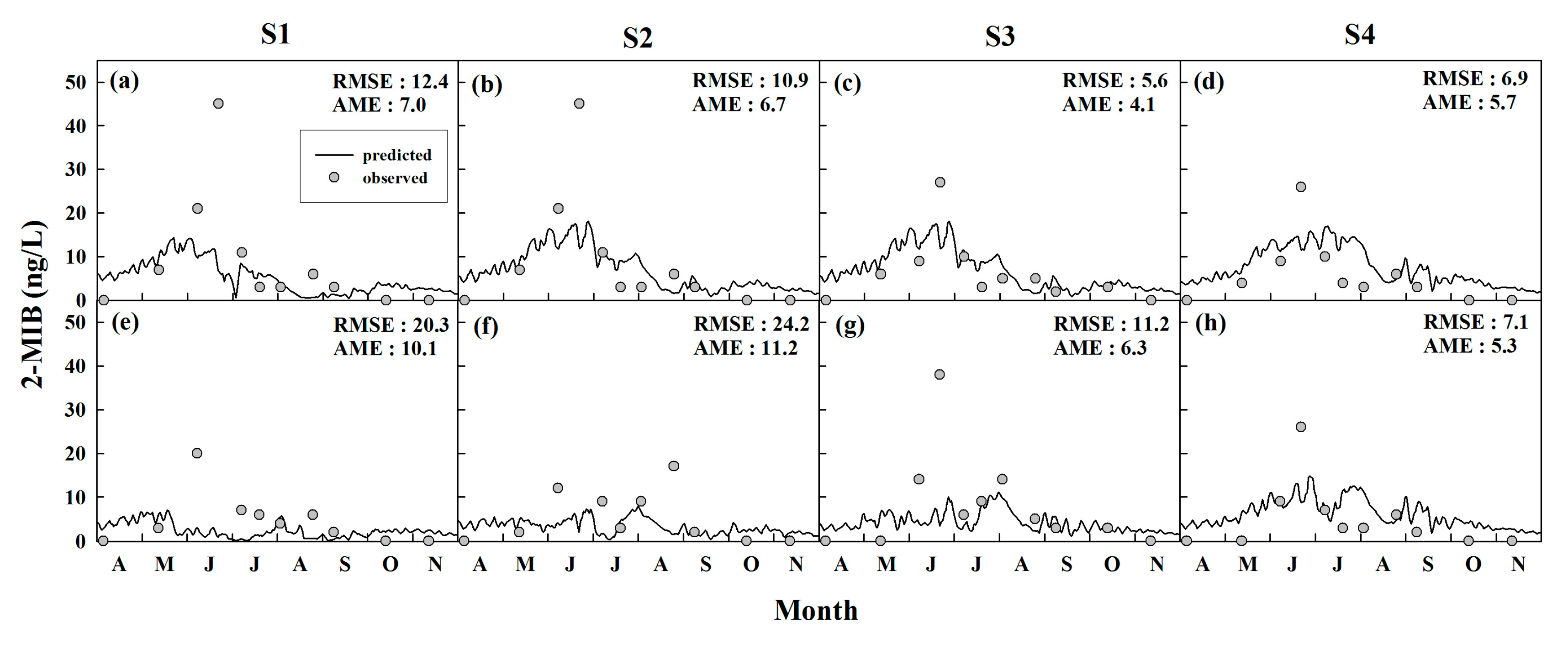
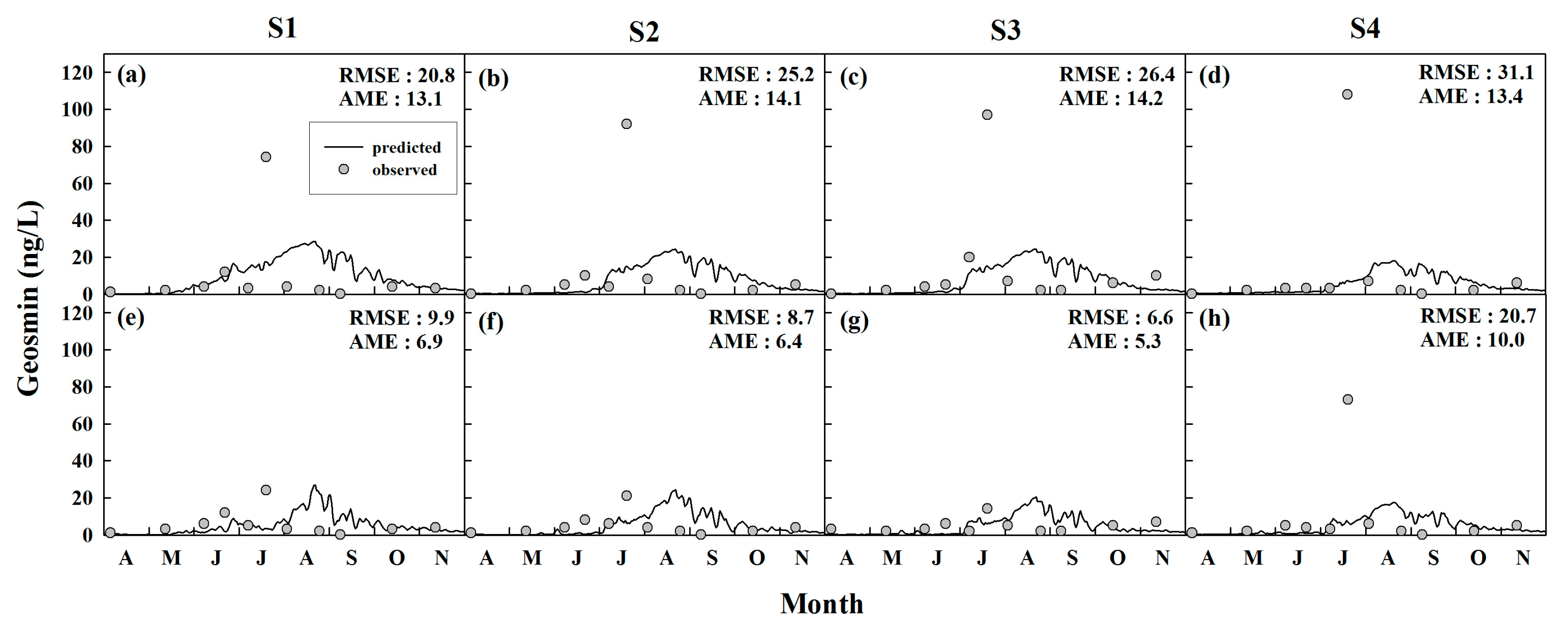
4.1.2. Algal-Derived Taste and Odor Compounds

The experimental values derived in the previous study were adopted for the parameters related to algal-derived taste and odor compounds. The production of taste and odor compounds was calculated by using 162 ng/mg algae, which was the result of a culture experiment for the Nakdong River samples in 2015 (Table 5). In that experiment, where mixed algal species were cultured, 2-MIB and geosmin had almost the same average concentration of 5 × 10⁻³ ng/cell [50]. While the experimental result was converted into a model parameter, the ratio of carbon to chlorophyll-a was calculated by applying the calibration factor of 40 mgC/mgChl-a (Table 3). In many studies, the potential for phytoplankton to produce taste and odor compounds have been calculated as varying widely. Watson et al. [13] provided a list of estimated per capita geosmin and 2-MIB production by cyanobacteria under different conditions, and reported that production of geosmin and 2-MIB vary considerably both among and within species. Jüttner and Watson [12] showed that Anabaena lemmermannii produced a total of 150 ng/mg (dry weight) geosmin under phosphorus-limited conditions and 500 ng/mg (dry weight) under phosphorus-rich conditions. Li et al. [51] estimated that the potential for Anabaena spiroides to produce geosmin was approximately 0.1 pg/cell in the Yanghe Lake, China. In Australia, Jones and Korth [52] showed that the production of geosmin by Anabaena sp. was 0.01 pg/cell, which was a very low concentration compared to the figure found by Li et al. Oh et al. [53] reported that Anabaena sp. produced extracellular geosmin at 1–2 pg/cell under different nitrogen concentrations. Wang et al. [42] estimated that production of 2-MIB by Psedanabaena sp. was 100–380 ng/μg Chl-a under variable temperature levels. Therefore, the parameter applied in this study was most similar to the values given in Jüttner and Watson [12] and Oh et al. [53]. When taste and odor compounds as algal metabolites were modeled, the model accurately simulated the overall concentrations of 2-MIB (Figure 6) and geosmin (Figure 7). The model simulation showed the highest concentration of 2-MIB for June. This agreed with the observation that 2-MIB had the highest concentration owing to the occurrence of Pseudanabaena sp. in June. Thus, the model appeared to predict the occurrence of 2-MIB. However, the highest concentration of the surface layer tended to be underestimated. The model errors for 2-MIB concentrations included an RMSE of 5.6–24.2 ng/L and an AME of 4.1–11.2 ng/L. S3–4 showed smaller errors than S1–2. The concentration of geosmin was also adequately predicted by the model. However, the model error had a larger range than that of 2-MIB (RMSE 6.6–31.1 ng/L, AME 5.3–13.4 ng/L). In particular, the occurrence of geosmin tended to be overestimated in August, when the water body was stabilized by low rainfall, and thus, Microcystis sp. was dominant. Since Microcystis sp. is not the main cause of geosmin, the model seems to have overestimated geosmin. Although the model predicted the geosmin and 2-MIB concentrations relatively well, its robustness may be limited due to the variability in the geosmin and 2-MIB productions based on specific species [12,13,51,52,53] and environmental factors such as light, temperature, and nutrients [17,36,41,42,54]. Depending on the variation of cyanobacteria species and hydrological and meteorological conditions, the concentration of taste and odor compounds can vary greatly. Thus, further study is needed to improve the model accuracy by obtaining additional data.

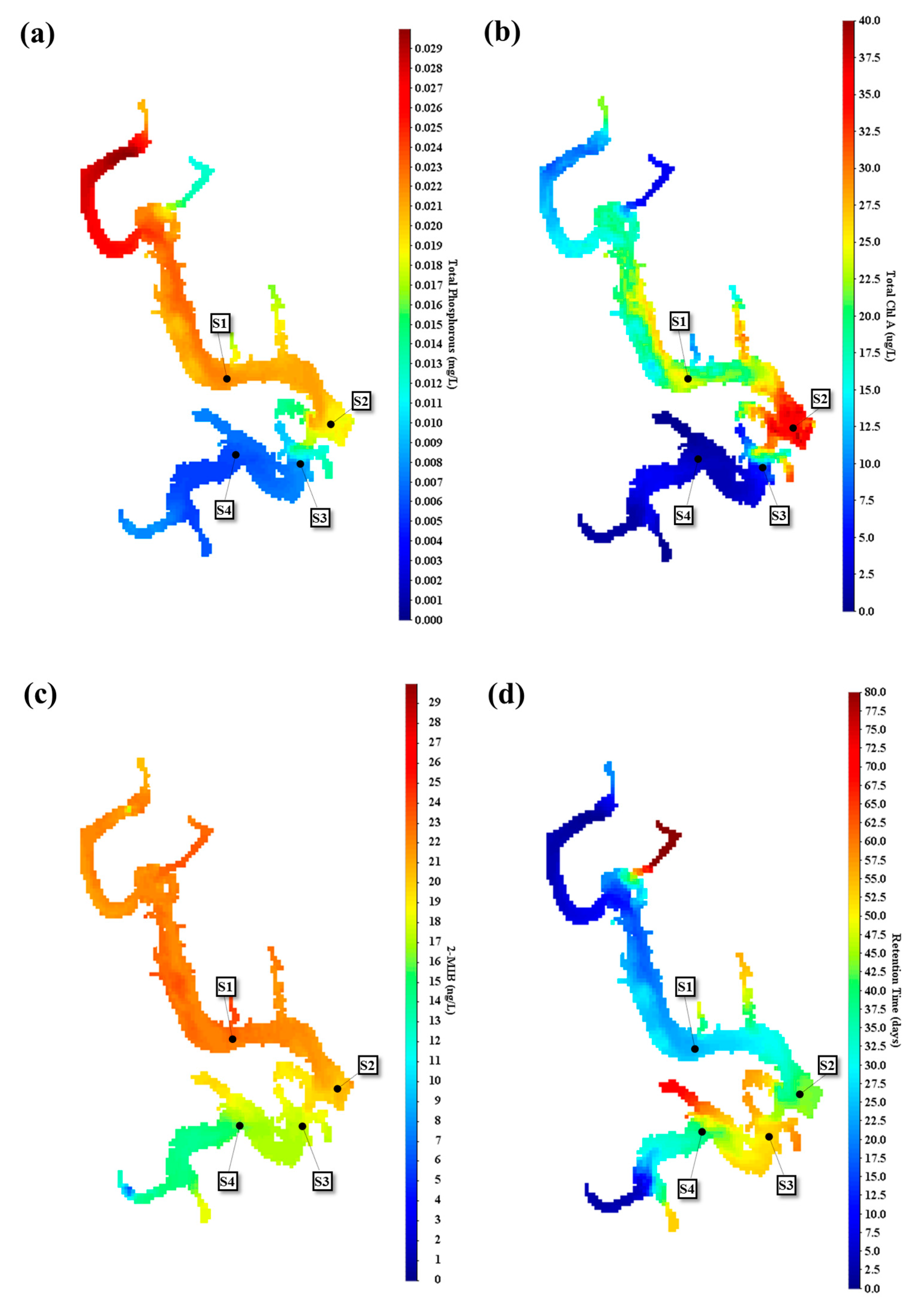
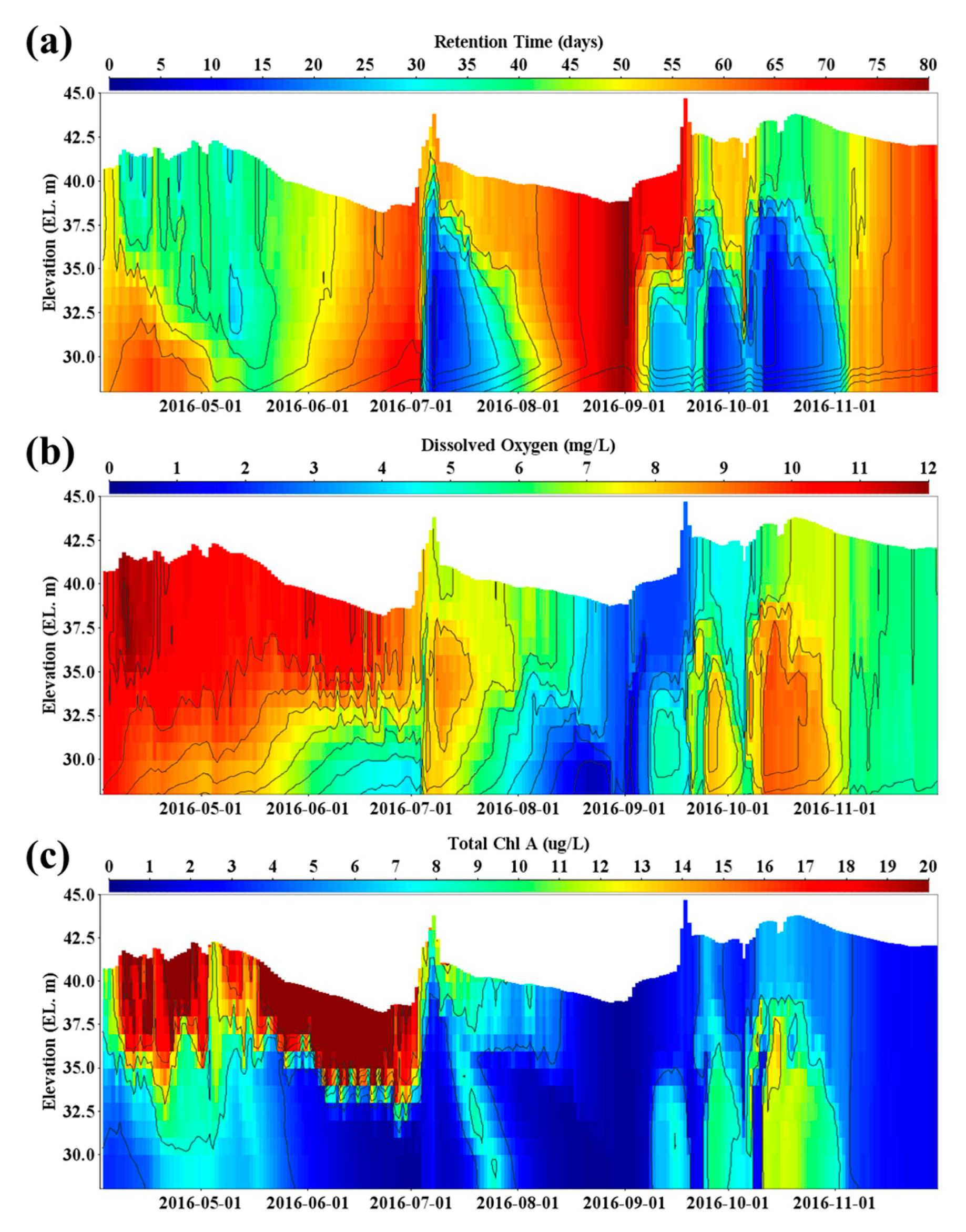
4.2. Effect of Spatiotemporal Physical–Water Quality Characteristics on the Occurrence of Taste and Odor Compounds

The occurrence of algae and taste and odor compounds at the Jinyang Reservoir was analyzed in a sophisticated manner (physically, physiochemically, and biologically) by utilizing the simulation results of the ELCOM–CAEDYM model. The concentrations of nutrients were greater in the Kyeongho River than in the Duckcheon River. The mouth of the Kyeongho River showed the highest concentration (Figure 8a), likely because the Kyeongho River has a larger basin area with many nutrients present (e.g., nitrogen, phosphorus); therefore, it is also likely that some zones had a high discharge of point and non-point sources of nutrients. The concentration of chlorophyll-a was high in front of the dam and the area of the Kyeongho River (Figure 8b). This indicates that influent water of the Kyeongho River, containing sufficient nutrients for algal growth, flows into the Jinyang Reservoir, and that this facilitates the growth of algae. Moreover, as the water body becomes more stable in front of the dam, algae grow excessively. On the other hand, the area including the Namgang Intake Tower (S3) showed better influent water quality than the Kyeongho River. However, S3 had a high frequency of algal growth and high concentrations of taste and odor compounds (Figure 8c). In particular, although S3 was only 2 km distant from S4, these two points showed remarkably different water quality characteristics. To analyze this phenomenon, hydraulic properties and its relevance to water quality, constituents such as nutrients were examined. Most notably, the nearby area of the Namgang Intake Tower (S3) had the longest retention time from a hydraulic perspective (Figure 8d). This was because the inflow of the Duckcheon River was only one fifth that of the Kyeongho River, owing to the difference in catchment area. Moreover, no discharge-derived flow was generated for geographical reasons. In other words, although the influent water quality from the Duchcheon River was relatively good, the retention time increased. For this reason, oxygen was depleted in the lower layer and algae occurred in the upper layer. Note, video for spatial and temporal distribution of water quality and taste and odor compounds in the Jinyang Reservoir was provided as supplementary material.
In particular, as was the case during the summer season (June to August) of 2016, if rainfall is low, water depth decreases and the water body continues to be stable; thermal stratification intensifies, preventing water layers from mixing. Consequently, oxygen is quickly depleted in the lower layer and the increasing water temperature results in an increased algal population. During this stagnant period, the amount of inflow from the Duckcheon River was low, and the high concentration of nutrients in the main stream of the Kyeongho River diffused into the intake tower area (Figure 8a). Hence, in a complicated way, this phenomenon appears to have facilitated the occurrence of algae and taste and odor compounds in the vicinity of the intake tower.
The results of a vertical water quality simulation were analyzed to examine the impact of prolonged retention time on DO depletion of the lower layer and algae growth in the area of the Namgang Dam Intake Tower (Figure 9). The result for other sites (S1, S3, S4) are reported in Figures S1–S3 as supplementary documents. When the amount of inflow and the water depth decreased in June and August, the retention time drastically increased and, significantly, increased more rapidly in the lower layer than in the upper layer (Figure 9a). The simulation accurately reproduced the phenomenon of drastically depleted DO in the lower layer during the period (Figure 9b). In addition, the model accurately predicted the period during which rainfall water depth increased, retention time decreased, and DO levels recovered. Figure 9c reveals that an increased retention time is closely related to times of algal growth. When the water body was stabilized due to increased retention time in June and from the middle of July to early August, the concentration of chlorophyll-a was high in the surface layer, and these periods coincided with the occurrence of geosmin and 2-MIB. Consequently, the Jinyang Reservoir as a shallow lake showed a large variation of water quality both temporally and spatially under the influence of hydrological factors (rainfall, inflow, outflow, etc.). When the water body was stabilized owing to low rainfall, high concentrations of algae and taste and odor compounds occurred, and the lower layer showed oxygen depletion.

5. Conclusions

This study attempted to establish a technique for predicting the occurrence of algae and algal-derived taste and odor compounds using a three-dimensional model that could reflect the complex physical properties of a shallow reservoir. The technique thus secured was intended to be utilized for dam operation and water treatment processes. A field survey was conducted and data were collected in order to identify spatiotemporal characteristics of water quality, algae, and taste and odor compounds and related causes. The ELCOM–CAEDYM model, a three-dimensional hydraulic and ecological model, was applied for simulation.
The occurrence of algae and taste and odor compounds was closely related to the hydrological and hydraulic characteristics of the Jinyang Reservoir. From June to August, when rainfall was low and the amount of inflow and outflow decreased remarkably, algal biomass increased. This period agreed with the time when the taste and odor compounds occurred. As for the taste and odor compounds, 2-MIB had its highest concentration of 80 ng/L in late June, and geosmin showed its highest concentration of 108 ng/L in the middle of July. In June, a high-concentration of 2-MIB occurred, owing to the appearance of Pseudanabaena sp., which is a cyanobacterium. From July to August, a high-concentration of geosmin occurred because of Anabaena sp., which resulted in problems in the water treatment process.
The coupled model of ELCOM and CAEDYM was applied to the Jinyang Reservoir in order to predict taste and odor compounds. Cyanobacteria groups producing either 2-MIB or geosmin were distinguished to enhance the accuracy of the model‘s predictions. The simulation showed that the spatial distribution and occurrence time of 2-MIB and geosmin were predicted relatively well. The model errors for 2-MIB concentrations included an RMSE of 5.6–24.2 ng/L and an AME of 4.1–11.2 ng/L; for geosmin, those values were an RMSE of 6.6–31.1 ng/L and an AME of 5.3–13.4 ng/L. However, the concentration of geosmin was overestimated for the period during which Microcystis sp. bloomed. Although the model predicted taste and odor compounds realistically for the Jinyang Reservoir in 2016, its robustness may be limited due to the variability in the unitary taste and odor compound productions based on specific species and environmental conditions [12,13,41,42,51,52,53,54]; the model also clusters cyanobacteria into two groups for taste and odor compound prediction, however, each species within each group could have different taste and odor compound productions and each species could bloom under very specific conditions [35,36,37,38,39,40,41,42,43,44], which the model cannot account for. Hence, future work will need to look at collecting more data and enhancing model functionalities in order to partially overcome such limitations and improve the model accuracy when applied to a new dataset with different input conditions.
When the impact of physical properties and water quality distribution on the occurrence of taste and odor compounds in the Jinyang Reservoir was analyzed, the nearby area of the Namgang wide area water supply intake tower showed the longest retention time for geographical and hydraulic reasons. Accordingly, despite relatively good influent water quality from the upper region, algae and taste and odor compounds occurred in high concentrations. The decrease in inflow and outflow, owing to low rainfall, not only had an immediate effect on the physical environment of the Jinyang Reservoir, but also played an important role in direct and indirect processes related to the occurrence of algae and taste and odor compounds, and the depletion of oxygen in the lower layer.

Supplementary Materials

The following are available online at https://www.mdpi.com/2073-4441/10/10/1396/s1: Figure S1: Temporal isopleth of vertical water quality in the Kyeongho River zone (S1): (a) retention time, (b) dissolved oxygen levels, (c) chlorophyll-a concentration; Figure S2: Temporal isopleth of vertical water quality in the Namgang wide-area water supply intake tower (S3): (a) retention time, (b) dissolved oxygen level, (c) chlorophyll-a concentration; Figure S3: Temporal isopleth of vertical water quality in the Duckcheon River zone (S4): (a) retention time, (b) dissolved oxygen level, (c) chlorophyll-a concentration, Video S1: Temporal and spatial distribution of water quality and taste and odor compounds in the Jinyang Reservoir.

Author Contributions

S.C. performed data analysis, model application and simulation; H.L. analyzed the algae data; K.-G.A. led the model application and supervised the study.

Funding

This research was supported by K-water (KIWE-WRRC-16-15).

Acknowledgments

The authors would like to thank the Yeonjeong Park in the K-water Convergence Institute and Younsam Kim in the Water Quality Analysis Center for supporting the algae analysis. The authors also extend their gratitude to all the members of the K-water—Namgang Office, Western Gyeongnam Office, and Water Quality Analysis Center—for participating in field monitoring and water quality analyses.

Conflicts of Interest

The authors declare no conflict of interest.

References

  1. Paerl, H.W.; Fulton, R.S.; Moisander, P.H.; Dyble, J. Harmful freshwater algal blooms, with an emphasis on cyanobacteria. Sci. World J. 2001, 1, 76–113. [Google Scholar] [CrossRef] [PubMed]
  2. Paerl, H.W.; Otten, T.G. Harmful cyanobacterial blooms: Causes, consequences, and controls. Microb. Ecol. 2013, 65, 995–1010. [Google Scholar] [CrossRef] [PubMed]
  3. Chorus, I.; Bartram, J. Toxic Cyanobacteria in Water: A Guide to Their Public Health Consequences, Monitoring and Management; World Health Organization: London, UK; New York, NY, USA, 1999; ISBN 0-419-23930-8. [Google Scholar]
  4. Smith, V.H.; Denlinger, J.S.; de Noyelles, F.; Campbell, S.; Pan, S.; Randtke, S.J.; Blain, G.T.; Strasser, V.A. Managing taste and odor problems in a eutrophic drinking water reservoir. J. Lake Reserv. Manag. 2002, 18, 319–323. [Google Scholar] [CrossRef]
  5. Watson, S.B. Aquatic taste and odor: A primary signal of drinking-water integrity. J. Toxicol. Environ. Health 2004, 67, 1779–1795. [Google Scholar] [CrossRef] [PubMed]
  6. Srinivasan, R.; Sorial, G.A. Treatment of taste and odor causing compounds 2-methyl isoborneol and geosmin in drinking water: A critical review. J. Environ. Sci. 2011, 23, 1–13. [Google Scholar] [CrossRef]
  7. Hsieh, W.H.; Chang, D.W.; Lin, T.F. Occurrence and removal of earthy-musty odorants in two waterworks in Kinmen Island, Taiwan. J. Hazard. Toxic Radioact. Waste 2014, 18, 04014012. [Google Scholar] [CrossRef]
  8. Korth, W. Determination of Odour Compounds in Surface Water. Ph.D. Thesis, University of Wollongong, Wollongong, Australia, July 1992. [Google Scholar]
  9. Izaguirre, G.; Taylor, W.D. A Psedanabaena species from Castaic Lake, California, that produce 2-methylisoborneol. Water Res. 1998, 5, 1673–1677. [Google Scholar] [CrossRef]
  10. Watson, S.B. Cyanobacterial and eukaryotic algal odour compounds: Signal or by-product? A review of their biological activity. Phycologia 2003, 42, 332–350. [Google Scholar] [CrossRef]
  11. Smith, J.L.; Boyer, G.L.; Zimba, P.V. A review of cyanobacterial odorous and bioactive metabolites: Impacts and management alternatives in aquaculture. Aquaculture 2008, 280, 5–20. [Google Scholar] [CrossRef]
  12. Jüttner, F.; Watson, S.B. Biochemical and ecological control of geosmin and 2-Methylisoborneol in source waters. Appl. Environ. Microbiol. 2007, 73, 4395–4406. [Google Scholar] [CrossRef] [PubMed]
  13. Watson, S.B.; Monis, P.; Baker, P.; Giglio, S. Biochemistry and genetics of taste- and odor-producing cyanobacteria. Harmful Algae 2016, 54, 112–127. [Google Scholar] [CrossRef] [PubMed]
  14. Zhang, K.; Lin, T.F.; Zhang, T.; Li, C.; Gao, N. Characterization of typical taste and odor compounds formed by Microcystis aeruginosa. J. Environ. Sci. 2013, 25, 1539–1548. [Google Scholar] [CrossRef]
  15. Otten, T.G.; Graham, J.L.; Harris, T.D.; Dreher, T.W. Elucidation of taste-and-odor producing bacteria and toxigenic cyanobacteria by shotgun metagenomics in a Midwestern drinking water supply reservoir. Appl. Environ. Microbiol. 2016, 82, 5410–5420. [Google Scholar] [CrossRef] [PubMed]
  16. Suurnäki, S.; Gomez-Saez, G.V.; Rantala-Ylinen, A.; Jokela, J.; Fewer, D.P.; Sivonen, K. Identification of geosmin and 2-methylisoborneol in cyanobacteria and molecular detection methods for the producers of these compounds. Water Res. 2015, 68, 56–66. [Google Scholar] [CrossRef] [PubMed]
  17. Su, M.; Yu, J.; Zhang, J.; Chen, H.; An, W.; Vogt, R.D.; Andersen, T.; Jia, D.; Wang, J.; Yang, M. MIB-producing cyanobacteria (Planktothrix sp.) in a drinking water reservoir: Distribution and odor producing potential. Water Res. 2015, 68, 444–453. [Google Scholar] [CrossRef] [PubMed]
  18. Wang, Z.; Shao, J.; Xu, Y.; Yan, B.; Li, R. Genetic basis for geosmin production by the water bloom-forming cyanobacterium, Anabaena ucrainica. Water 2015, 7, 175–187. [Google Scholar] [CrossRef]
  19. Westerhoff, P.M.; Hernandez, M.R.; Baker, L.; Sommerfeld, M. Seasonal occurrence and degradation of 2-methylisoborneol in water supply reservoirs. Water Res. 2005, 39, 4899–4912. [Google Scholar] [CrossRef] [PubMed]
  20. Dzialowski, A.R.; Smith, V.H.; Huggins, D.G.; de Noyelles, F.; Lim, N.C.; Baker, D.S.; Beury, J.H. Development of predictive models for geosmin-related taste and odor in Kansas, USA, drinking water reservoirs. Water Res. 2009, 43, 2829–2840. [Google Scholar] [CrossRef] [PubMed]
  21. Bradley, P.M. Environmental factors that influence cyanobacteria and geosmin occurrence in reservoirs. In Current Perspectives in Contaminant Hydrology and Water Resources Sustainability; Journey, C.A., Beaulieu, K.M., Bradley, P.M., Eds.; InTech: Rijeka, Croatia, 2013; pp. 27–54. [Google Scholar]
  22. Parinet, J.; Rodriguez, M.J.; Sérodes, J.B. Modelling geosmin concentrations in three sources of raw water in Quebec, Canada. Environ. Monit. Assess. 2013, 185, 95–111. [Google Scholar] [CrossRef] [PubMed]
  23. Bruder, S.R. Prediction of Spatial-Temporal Distribution of Algal Metabolites in Eagle Creek Reservoir, Indianapolis, IN. Master’s Thesis, Indiana University, Indianapolis, October 2012. [Google Scholar]
  24. Harris, T.D.; Graham, J.L. Predicting cyanobacterial abundance, microcystin, and geosmin in a eutrophic drinking-water reservoir using a 14-year dataset. Lake Reserv. Manag. 2017, 33, 32–48. [Google Scholar] [CrossRef]
  25. Chung, S.W.; Imberger, J.; Hipsey, M.R.; Lee, H.S. The influence of physical and physiological processes on the spatial heterogeneity of a Microcystis bloom in a stratified reservoir. Ecol. Model. 2014, 289, 133–149. [Google Scholar] [CrossRef]
  26. Robson, B.J.; Hamilton, D.P. Three-dimensional modelling of a Microcystis bloom event in the Swan River estuary, Western Australia. Ecol. Model. 2004, 174, 203–222. [Google Scholar] [CrossRef]
  27. Leon, L.F.; Smith, R.E.; Hipsey, M.R.; Bocaniov, S.A.; Higgins, S.N.; Hercky, R.E.; Antenucci, J.P.; Imberger, J.A.; Guildford, S.J. Application of a 3D hydrodynamic–biological model for seasonal and spatial dynamics of water quality and phytoplankton in Lake Erie. J. Great Lakes Res. 2011, 37, 41–53. [Google Scholar] [CrossRef]
  28. Yajima, H.; Choi, J. Changes in phytoplankton biomass due to diversion of an inflow into the Urayama Reservoir. Ecol. Eng. 2013, 58, 180–191. [Google Scholar] [CrossRef]
  29. Islam, M.N.; Kitazawa, D.; Park, H.D. Numerical modeling on toxin produced by predominant species of cyanobacteria within the ecosystem of Lake Kasumigaura, Japan. Procedia Environ. Sci. 2012, 13, 166–193. [Google Scholar] [CrossRef]
  30. Chung, S.W.; Chong, S.A.; Park, H.S. Development and applications of a predictive model for geosmin in North Han River, Korea. Procedia Eng. 2016, 154, 521–528. [Google Scholar] [CrossRef]
  31. APHA. Standard Methods for the Examination of Water and Wastewater, 20th ed.; American Public Health Association: Washington, DC, USA, 1998. [Google Scholar]
  32. Korea Meteorological Administration (KMA). Available online: http://www.weather.go.kr/weather/index.jsp (accessed on 1 May 2018).
  33. Hodges, B.R.; Dallimore, C. Estuary, Lake and Coastal Ocean Model: ELCOM. v2.2 Science Manual; University of Western Australia Technical Publication: Perth, Australia, 2006; pp. 1–32. [Google Scholar]
  34. Hipsey, M.R.; Romero, J.R.; Antenucci, J.P.; Hamilton, D. Computational Aquatic Ecosystem Dynamics Model: CAEDYM v2.3 Science Manual; University of Western Australia Technical Publication: Perth, Australia, 2006; pp. 36–54. [Google Scholar]
  35. Nalewajko, C.; Murphy, T.P. Effects of temperature, and availability of nitrogen and phosphorus on the abundance of Anabaena and Microcystis in Lake Biwa, Japan: An experimental approach. Limnology 2001, 2, 45–48. [Google Scholar] [CrossRef]
  36. Li, Z.; Hobson, P.; An, W.; Burch, M.; House, J.; Yang, M. Earthy odor compounds production and loss in three cyanobacterial cultures. Water Res. 2012, 46, 5165–5173. [Google Scholar] [CrossRef] [PubMed] [Green Version]
  37. Cai, Y.; Kong, F. Diversity and dynamics of picocyanobacteria and the bloom-forming cyanobacteria in a large shallow eutrophic lake (lake Chaohu, China). J. Limnol. 2013, 72, e38. [Google Scholar] [CrossRef]
  38. Mowe, M.; Mitrovic, S.; Lim, R.; Furey, A.; Yeo, D. Tropical cyanobacterial blooms: A review of prevalence, problem taxa, toxins and influencing environmental factors. J. Limnol. 2014, 74. [Google Scholar] [CrossRef]
  39. Li, X.; Dreher, T.W.; Li, R. An overview of diversity, occurrence, genetics and toxin production of bloom-forming Dolichospermum (Anabaena) species. Harmful Algae 2016, 54, 54–68. [Google Scholar] [CrossRef] [PubMed]
  40. Lu, X.; Tian, C.; Pei, H.; Hu, W.; Xie, J. Environmental factors influencing cyanobacteria community structure in Dongping Lake, China. J. Environ. Sci. 2013, 25, 2196–2206. [Google Scholar] [CrossRef]
  41. Kakimoto, M.; Ishikawa, T.; Miyagi, A.; Saito, K.; Miyazaki, M.; Asaedaa, T.; Yamaguchi, M.; Uchimiya, H.; Yamada, M. Culture temperature affects gene expression and metabolic pathways in the 2-methylisoborneol-producing cyanobacterium Pseudanabaena galeata. J. Plant Physiol. 2014, 171, 292–300. [Google Scholar] [CrossRef] [PubMed]
  42. Wang, Z.; Li, R. Effects of light and temperature on the odor production of 2-Methylisoborneol-producing Pseudanabaena sp. and geosmin-producing Anabaena ucrainica (cyanobacteria). Biochem. Syst. Ecol. 2015, 58, 219–226. [Google Scholar] [CrossRef]
  43. Zhaoa, H.; Wang, Y.; Yang, L.; Yuan, L.; Peng, D. Relationship between phytoplankton and environmental factors inlandscape water supplemented with reclaimed water. Ecol. Indic. 2015, 58, 113–121. [Google Scholar] [CrossRef]
  44. Rosińska, J.; Kozak, A.; Dondajewska, R.; Gołdyn, R. Cyanobacteria blooms before and during the restoration process of a shallow urban lake. J. Environ. Manag. 2017, 198, 340–347. [Google Scholar] [CrossRef] [PubMed]
  45. Chung, S.W.; Hipsey, M.R.; Imberger, J. Modelling the propagation of turbid density inflows into a stratified lake: Daecheong Reservoir, Korea. Environ. Model. Softw. 2009, 24, 1462–1482. [Google Scholar] [CrossRef]
  46. Vilhena, L.C.; Hillmer, I.; Imberger, J. The role of climate change in the occurrence of algal blooms: Lake Burragorang, Australia. Limnol. Oceanogr. 2010, 55, 1188–1200. [Google Scholar] [CrossRef] [Green Version]
  47. Linden, L.; Daly, R.I.; Burch, M.D. Suitability of a coupled hydrodynamic water quality model to predict changes in water quality from altered meteorological boundary conditions. Water 2015, 7, 348–361. [Google Scholar] [CrossRef]
  48. Westernhagen, N.V. Measurements and Modelling of Eutrophication Processes in Lake Rotoiti, New Zealand. Ph.D. Thesis, The University of Waikato, Hamilton, New Zealand, 2010. [Google Scholar]
  49. Missaghi, S.; Hondzo, M. Evaluation and application of a three-dimensional water quality model in a shallow lake with complex morphometry. Ecol. Model. 2010, 221, 1512–1525. [Google Scholar] [CrossRef]
  50. K-Water. Development of the Predictive Model and Analysis of Occurrence Characteristics for T&Os in Nakdong River; Korea Water Resources Corporation (K-Water) Technical Report; K-Water: Daejeon, Korea, 2015; pp. 46–54. [Google Scholar]
  51. Li, Z.; Yu, J.; Yang, M.; Zhang, D.; Burch, M.D.; Han, W. Cyanobacterial population and harmful metabolites dynamics during a bloom in Yanghe Reservoir, North China. Harmful Algae 2010, 9, 481–488. [Google Scholar] [CrossRef] [Green Version]
  52. Jones, G.J.; Korth, W. In situ production of volatile odor compounds by river and reservoir phytoplankton populations in Australia. Water Sci. Technol. 1995, 31, 145–153. [Google Scholar] [CrossRef]
  53. Oh, H.S.; Lee, C.S.; Srivastava, A.; Oh, H.M.; Ahn, C.Y. Effects of environmental factors on cyanobacterial production of odorous compounds: Geosmin and 2-methylisoborneol. J. Microbiol. Biotechnol. 2017, 27, 1316–1323. [Google Scholar] [CrossRef] [PubMed]
  54. Bertone, E.; Burford, M.A.; Hamilton, D.P. Fluorescence probes for real-time remote cyanobacteria monitoring: A review of challenges and opportunities. Water Res. 2018, 141, 152–162. [Google Scholar] [CrossRef] [PubMed]
Figure 1. (a) Location of the Namgang Dam (Jinyang Reservoir); (b) Bathymetric map of the Jinyang Reservoir including the location of water quality monitoring sites and intake towers. The scale of the color bar scale is in units of elevation meter (EL. m).
Water 10 01396 g001
Figure 2. Populations of algae at each monitoring point in the Jinyang Reservoir: (a) upper layer, (b) middle layer. Dominant species are marked on each bar graph. (CRY: Cryptomonas, GEI: Geitlerinema, SYN: Synedra, PSE: Pseudanabaena, EUD: Eudorina, MIC: Microcystis, AUL: Aulacoseira, RHO: Rhodomonas, COE: Coelastrum).
Water 10 01396 g002
Figure 3. Observed concentrations of (a) chlorophyll-a (Chl-a), (b) 2-methylisoborneol (2-MIB), and (c) geosmin in the upper, middle, and lower layers of each monitoring point in the Jinyang Reservoir.
Water 10 01396 g003
Figure 4. Relationship between (a) 2-MIB concentration and Pseudanabaena sp. abundance and (b) geosmin concentration and Anabaena sp. abundance in the Jinyang Reservoir.
Water 10 01396 g004
Figure 5. Comparison of predicted and observed dissolved oxygen (DO), nitrate, total organic carbon (TOC), total phosphorus (TP), and Chl-a concentrations at S1 (ae), S2 (fj), S3 (km), and S4 (nr). The quantitative model errors calculated are given in Table 4.
Water 10 01396 g005
Figure 6. Predicted and observed 2-MIB concentrations at S1–S4: (a)–(d) upper; (e)–(h) middle.
Water 10 01396 g006
Figure 7. Predicted and observed geosmin concentrations at S1–S4; (a)–(d) upper; (e)–(h) middle.
Water 10 01396 g007
Figure 8. Spatial distribution of water quality and taste and odor compounds during algal bloom occurrence (21 June 2016): (a) TP, (b) chlorophyll-a, (c) 2-MIB, and (d) retention time.
Water 10 01396 g008
Figure 9. Temporal isopleth of vertical water quality in front of the Namgang dam (S2): (a) retention time, (b) DO, (c) chlorophyll-a.
Water 10 01396 g009
Table 1. Monthly meteorological and hydrological data for the Namgang Dam in 2016 and comparison with past data.
MonthMeteorological DataHydrological Data
Monthly Average
Air Temperature (°C)
Rainfall (mm)Monthly Average
Inflow (m3/s)
Monthly Average
Outflow (m3/s)
20161981–2010 (1)20161981–201020161976–2015 (2)20161976–2015
January−0.2−0.135.432.916.711.925.913.6
February2.72.176.443.036.318.725.418.0
March7.96.8121.072.162.428.963.529.1
April13.912.8299.7118.2110.546.2102.641.7
May18.217.6153.9122.865.142.487.148.0
June21.921.5113.8213.020.775.133.878.4
July25.625.1161.0300.0118.6192.0109.7186.3
August26.725.774.8316.917.2201.128.3199.2
September21.521.0407.5184.5106.2131.075.6133.8
October16.014.5170.145.0128.229.0121.733.2
November8.37.737.045.020.119.632.418.5
December3.22.084.019.234.215.828.017.5
(1) Climatological normal (KMA [32]), (2) Period after dam construction and operation.
Table 2. Hydraulic parameters used in the estuary, lake, and coastal ocean model (ELCOM) for the Jinyang Reservoir.
ParametersVariableUnitAssigned ValueReference
Horizontal eddy diffusivityDXm2/s1
Bottom drag coefficientCD 0.0050.005 1)
Extinction coefficient for NIR (700–2000 nm)λNIR/m11 1)
Extinction coefficient for PAR (400–700 nm)λPAR/m0.250.25 1)
Extinction coefficient for UVA (320–400 nm)λUVA/m11 1)
Extinction coefficient for UVB (300–320 nm)λUVB/m11 1)
Mean albedo for short-wave radiationαSW 0.080.08 1)
Sources: 1) Chung et al. [45].
Table 3. Water quality parameters applied in the computational aquatic ecosystem dynamic model (CAEDYM) for the Jinyang Reservoir.
ParameterDescriptionUnitAssigned ValueReference
CYANO1CYANO2FDIAT
Phytoplankton parametersμmaxMaximum specific growth rate/day0.50.51.21.1 1)–1.22)
YccAverage ratio of C to Chl-amg-C/mg-Chl.a40402040 1)
IStLight saturation for max. productionuE/m2/s13013070100 2)–130 1)
KpaHalf saturation constant for Pmg/L0.0050.0050.0050.008 1),2)
KnaHalf saturation constant for Nmg/L0.0450.0450.0500.030 2)
KCaHalf saturation constant for Cmg/L222-
KsaHalf saturation constant for Simg/L000.15-
INmin/maxMin/max internal N concentrationmg-N/mg-Chl.a2.0/4.02.0/4.02.0/4.0-
IPmin/maxMin/max internal P concentrationmg-P/mg-Chl.a0.1/0.60.1/0.60.1/0.6-
ICmin/maxMin/max internal C concentrationmg-C/mg-Chl.a15/8015/8015/80-
vTTemperature multiplier for growth-1.061.061.061.07 2)
TstaStandard temperatureoC20.020.020.020.0 1),2)
ToptOptimum temperatureoC24.526.018.022.0 2)–30.0 1)
TmaxMaximum temperatureoC32.036.032.035.0 2)–39.0 1)
krRespiration rate coefficient/day0.120.120.080.070 1)–0.1 2)
vRTemperature multiplier for respiration-1.081.081.08-
Nutrient parameterskoN2Denitrification rate coefficient (20 °C)/day0.010.03 3)–0.15 4)
KN2Inverted half-saturation constant for effect of oxygen on denitrificationmg/L0.50.44 4)
vONTemperature multiplier for denitrification-1.081.08 3)
koNHNitrification rate coefficient (20 °C)/day0.0500.065 3) –0.25 4)
KOnHalf-saturation constant for effect of oxygen on nitrificationmg/L20.5 3) –0.75 4)
vN2Temperature multiplier for nitrification-1.081.08 1)
PON1maxRate coefficient of PONL to DONL (20 °C)/day0.0100.003 3) –0.005 4)
DON1maxRate coefficient of DONL to NH4 (20 °C)/day0.0030.008 3) –0.08 4)
POP1maxRate coefficient of POPL to DOPL (20 °C)/day0.010.02 3) –0.03 4)
DOP1maxRate coefficient of DOPL to PO4 (20 °C)/day0.0050.025 3) –0.25 4)
Sources: 1) Vilhena et al. [46], 2) Linden et al. [47], 3) Westernhagen [48], 4) Missaghi and Hondzo [49].
Table 4. Modeling errors for each point and water quality constituents in the Jinyang Reservoir.
VariablesRoot-Mean-Square Error (RMSE)Absolute Mean Error (AME)
S1S2S3S4S1S2S3S4
DO (mg/L)2.72.52.73.42.11.92.22.8
NO3-N (mg/L)0.3210.2740.2430.2130.2790.2370.2090.182
TOC (mg/L)0.80.8-0.70.60.5-0.4
TP (mg/L)0.0160.009-0.0140.0130.006-0.010
Chl-a (μg/L)13.49.811.78.510.67.48.66.3
Table 5. Parameters applied for estimating algal metabolites at the Jinyang Reservoir.
ParametersVariableUnitAssigned Value
Degradation rate constant m x /d0.14
Minimum internal metabolite concentration I X a M I N mg / L mgChla / L 0
Internal metabolite concentration during maximum production I X a M A X mg / L mgChla / L 0.00324

