Article

Simulating Hydrological Impacts under Climate Change: Implications from Methodological Differences of a Pan European Assessment

by
Aristeidis G. Koutroulis
1,*,
Lamprini V. Papadimitriou
2,
Manolis G. Grillakis
1,
Ioannis K. Tsanis
1,
Klaus Wyser
3,
John Caesar
4 and
Richard A. Betts
4,5
1
School of Environmental Engineering, Technical University of Crete—TUC, Chania 73100, Greece
2
Cranfield Water Science Institute, Cranfield University, Cranfield MK43 0AL, UK
3
Rossby Centre, SMHI, 601 76 Norrköping, Sweden
4
Met Office Hadley Centre, FitzRoy Road, Exeter EX1 3PB, UK
5
Global Systems Institute, University of Exeter, Exeter EX4 4QE, UK
*
Author to whom correspondence should be addressed.
Water 2018, 10(10), 1331; https://doi.org/10.3390/w10101331
Submission received: 7 August 2018 / Revised: 20 September 2018 / Accepted: 24 September 2018 / Published: 26 September 2018
(This article belongs to the Section Hydraulics and Hydrodynamics)

Abstract

:
The simulation of hydrological impacts in a changing climate remains one of the main challenges of the earth system sciences. Impact assessments can be, in many cases, laborious processes leading to inevitable methodological compromises that drastically affect the robustness of the conclusions. In this study we examine the implications of different CMIP5-based regional and global climate model ensembles for projections of the hydrological impacts of climate change. We compare results from three different assessments of hydrological impacts under high-end climate change (RCP8.5) across Europe, and we focus on how methodological differences affect the projections. We assess, as systematically as possible, the differences in runoff projections as simulated by a land surface model driven by three different sets of climate projections over the European continent at global warming of 1.5 °C, 2 °C and 4 °C relative to pre-industrial levels, according to the RCP8.5 concentration scenario. We find that these methodological differences lead to considerably different outputs for a number of indicators used to express different aspects of runoff. We further use a number of new global climate model experiments, with an emphasis on high resolution, to test the assumption that many of the uncertainties in regional climate and hydrological changes are driven predominantly by the prescribed sea surface temperatures (SSTs) and sea-ice concentrations (SICs) and we find that results are more sensitive to the choice of the atmosphere model compared to the driving SSTs. Finally, we combine all sources of information to identify robust patterns of hydrological changes across the European continent.

1. Introduction

Climate change impact studies are largely based on climatic projections simulated by climate models. The impact modeling process can in many cases be computationally demanding, making the use of data from all models available within large-scale projects, such as the Coupled Model Inter-comparisons Project Five (CMIP5), practically impossible. This inevitably leads to compromises in terms of the number of models used. These constraints, combined with the need for the most representative sample, have led to the development of methods for the identification of fewer representative models [1,2]. These models constitute a subset of a larger model ensemble and are considered to account for a significant space of the potential climate changes as simulated by the total ensemble, with the benefit of reducing the number of laborious impact simulations. However, downsizing of the ensemble involves several risks, such as omitting part of the uncertainty of the original ensemble and skewing regional or seasonal climate change signals towards the model subset [3].
Despite the climate modeling advances moving from the CMIP3 to the CMIP5 experiment [4] the need for further downscaling, especially in the case of regional-scale studies, is still apparent. The dynamical downscaling using finer resolution regional climate models (RCMs) or GCMs is computationally expensive [5] and introduces additional sources of uncertainty stemming from the physical parameterization of the downstream models [6]. Further uncertainties, that can also lead to the modification of climate model signals, are exposed by the use of bias adjustment [7], which in some cases is a necessary step when it comes to supporting impact study modeling [8,9,10,11]. In addition, the way of interpreting climate change projections and impacts, typically in terms of model spread at the grid point instead of physically consistent model based patterns, often leads to inflation of uncertainty, especially in the case of multi-model subsets [12].
Focusing on hydrological impact modeling, several studies have come to the conclusion that the choice of the climate model projection has a larger influence on the hydrologic output than the selection of the emission pathway [13,14,15] and the bias correction method [16]. The structure of the hydrologic model can also play a significant role in the projected changes [17]. Thus, the methodological context of any impact study has a direct impact on the projected outcome, the communicated message and the decisions that arise based on the information provided. It is therefore of utmost importance for the results and potential sources of uncertainty of every impact study to be critically assessed, by comparing them to the range of impacts resulting from the current state of science.
From this perspective, the objectives of this study are twofold. Firstly, to investigate how the methodological differences between commonly used approaches to making climate projections and studying impacts affect the hydrologic projections and hence the robustness of the study’s findings. In this context we examine, as systematically as possible, the differences in hydrological response over Europe as simulated by a land surface model driven by different sets of climate projections. This approach will not quantify the full range of sources of uncertainty in projections, because we still rely on a single land surface model, so responses on land-atmosphere interactions are constrained by the parametrization of that single model. Nevertheless, we are not focusing on that aspect and our experimental setup allows some of the uncertainties between commonly used approaches in climate-change impacts to be illustrated and explored. Secondly, we are using a number of new global climate model experiments, with an emphasis on high resolution, to test the assumption that many of the uncertainties about regional climate (and therefore hydrological) changes are driven predominantly by the prescribed boundary conditions, and specifically sea surface temperature (SST). Finally, we combine all sources of information to identify robust patterns of hydrological changes over the European continent at global warming of 1.5 °C, 2 °C and 4 °C relative to pre-industrial levels, according to the RCP8.5 concentration scenario.

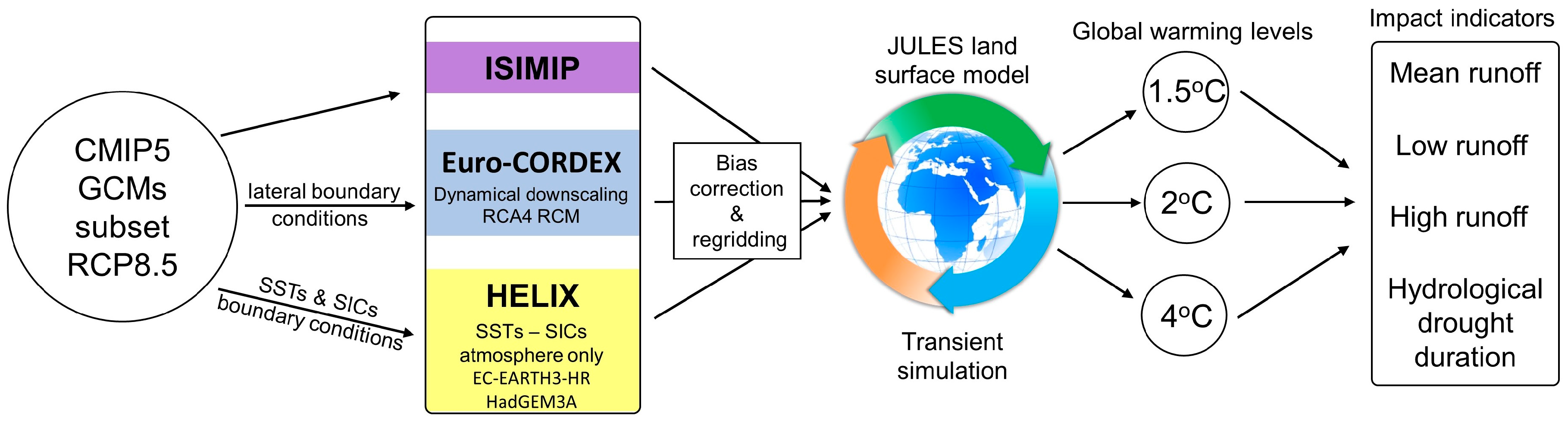
2. Materials and Methods

The fifth phase of the Coupled Model Intercomparison Project (CMIP5) [18] is currently the basis of climate modeling and climate change impact research. The CMIP5 ensemble consists of 25 to 42 climate simulations, depending on the representative concentration pathway (RCP) scenario [19]. Climate change impact assessments are usually limited to a small number of “representative” CMIP5 simulations in order to reduce modeling effort. The Inter-sectoral Impact Model Inter-comparison Project (ISIMIP) [20] is, for example, a well-established consistent framework of multi-sectoral impact assessment that is based on a subset of five CMIP5 models, used in global [21] and regional [22] scale studies.
The coarse resolution of a typical CMIP5 GCM limits the ability to simulate regional-scale climates. Regional climate models (RCMs), operating at higher resolution, are filling this gap by providing more detailed spatial information [23]. The Euro-CORDEX [24] is an example of a high-resolution regional climate change ensemble downscaled for Europe, that results in substantially different projected changes compared to the driving GCMs.
However, the added value of the RCMs is highly dependent on the driving fields provided by the GCMs. While Euro-CORDEX simulations are at ~50 km and even ~12.5 km, the limited geographical area over which this high resolution is applied limits the degree to which an RCM can recreate small-scale activity not already present in the GCM boundary conditions [25]. Many studies also indicate that higher GCM resolution is necessary to accurately simulate the observed energy spectrum of the climate system [26,27,28,29]. To address the need for better information we use two higher spatial resolution GCMs, HadGEM3A [30,31] and EC-EARTH3-HR [32] driven by a subset of CMIP5 GCMs. These simulations are performed in the frame of a European funded project focusing on high-end climate impacts and extremes (HELIX) and hereinafter referred to as the HELIX ensemble. We then assess the robustness of hydrological impacts between the original CMIP5, using data for the European region from the global ISIMIP biophysical impacts projections, the Euro-CORDEX driven impacts, and the new climate projections as simulated by a land surface model. The methodological workflow of the study is illustrated in Figure 1.

2.1. Climate Model Ensembles

2.1.1. ISIMIP

The “fast-track” phase of ISIMIP project uses a consistent subset of five (5) GCMs from the CMIP5 experiment [20], listed in Table 1. The temporal resolution of the dataset is daily, spanning the years 1960 to 2099, and including part of the historical recent past and the projections for RCP8.5. Original GCM outputs are remapped on a 0.5° × 0.5° grid mesh. Eleven (11) variables are bias adjusted using a trend preserving bias correction method [33] against a land only global coverage observational dataset [34] for the 1960 to 1999 reference period. The representativeness of these models compared to the spread of projections within the CMIP5 dataset is described by McSweeney and Jones [19].

2.1.2. Euro-CORDEX

The European initiative Euro-CORDEX, part of the wider Coordinated Regional Downscaling Experiment (WCRP), provides regional climate simulations for Europe driven by a number of CMIP5 GCMs. Climate datasets are available at horizontal resolutions of 50 km (EUR-44) and 12.5 km (EUR-11) [24] depending on the model. Five (5) of the EURO-CORDEX climate scenarios were used for the current assessment (Table 1). The model selection was made based on two requirements: First, that the driving GCM has been also used in ISIMIP runs so as to compare the two configurations; and second, that the GCM data have been downscaled to the 0.44 degree grid. Three of the five scenarios selected use the same driving GCM (GFDL-ESM2M, NorESM1-M and HadGEM2-ES). For the rest, downscaled data were not available and the most similar GCM was selected instead (MIROC5 instead of MIROC-ESM-CHEM and IPSL-CM5A-MR instead of IPSL-CM5A-LR). All five GCMs have been downscaled with the same RCM, namely RCA4 [35], which could result in a bias toward the RCM parameterization. Climate variables are bias adjusted using a quantile mapping methodology [36] against the E-OBS dataset [37].

2.1.3. HELIX AGCMs

New higher resolution climate projections are produced by two Atmosphere Global Climate Models (AGCMs) EC-EARTH3-HR and HadGEM3A (Global Atmosphere 6.0), with prescribed time varying SSTs and sea ice, provided by a range of CMIP5 climate models (Table 1), in the frame of a European funded project focusing on high-end climate impacts and extremes (HELIX). The HELIX AGCMs hi-res ensemble was generated as described in Wyser et al. [38] and used in the recent studies by Alfieri et al. [39] and Shannon et al. [40]. The criterion for model selection was to cover a wide range of uncertainty in the future climate projections. The two climate models of the next generation with horizontal resolution of 30–60 km are transition versions of those currently being used in upcoming CMIP6 experiments. This higher resolution ensemble of projections will be referred to as the HELIX ensemble. By using an atmosphere only experimental setup, we are able to cover the maximum range of possible regional climate changes within limited computing resources. Prescribing SSTs and SICs allow our results to be easily compared with other studies from the climate science community (common ISIMIP and Euro-CORDEX models), and in particular with the climate and climate change projected by the forcing CMIP5 models, to assess the benefits of adopting a higher resolution. Climate model outputs are remapped in a common 0.5° × 0.5° grid and bias adjusted against the PGFv2 dataset [41] using the ISIMIP trend preserving bias correction method [33].

2.2. Hydrological Modeling

The above-mentioned climate model ensembles were used to drive the JULES land surface model [42,43] providing changes in future runoff. Two JULES setups were used in this study. The ISIMIP-based runs were already performed in the frame of the ISIMIP Fast Track [20] multi-model experiment as described in detail by Davie et al. [44]. The model was run at the native resolution of the HadGEM2-ES (1.875 degree longitude by 1.25 degree latitude) and the runoff outputs were regridded to 0.5° × 0.5°. The model run started from a 1950 dump file from a HadGEM2-ES historical run and ran for 5 spin up cycles of 30 years. Next, the model was run for 185 years using dynamic (standard) TRIFFID and increasing CO2 concentrations [45].
The Euro-CORDEX and HELIX simulations were performed with versions 4.1 and 4.3 of JULES, respectively [46,47]. The JULES name lists of the abovementioned simulations can be downloaded at https://github.com/w0rldview/jules-w1_namelists. The spatial resolution used was that of the native climate data—0.44° grid for Euro-CORDEX and 0.5° grid for HELIX. Other JULES set up were common between the two runs in configuration JULES_W1 as used in the ISIMIP2A project [8]. The model was spun up with ten spin up cycles of one year (1971–1972), and additionally the first ten years of simulations (1971–1980) were discarded as an extended spin up period. Vegetation was kept static (TRIFFID disabled) and CO2 concentrations were annually varying.
The different model configurations used in the ISIMIP simulations compared to the Euro-CORDEX and HELIX simulations might introduce an impact model bias to the results. Enabled (in ISIMIP simulations) versus disabled (in Euro-CORDEX and HELIX) dynamic vegetation, together with different parameterizations in the two configurations, might make a difference to the hydrological outputs which has not been explicitly quantified.

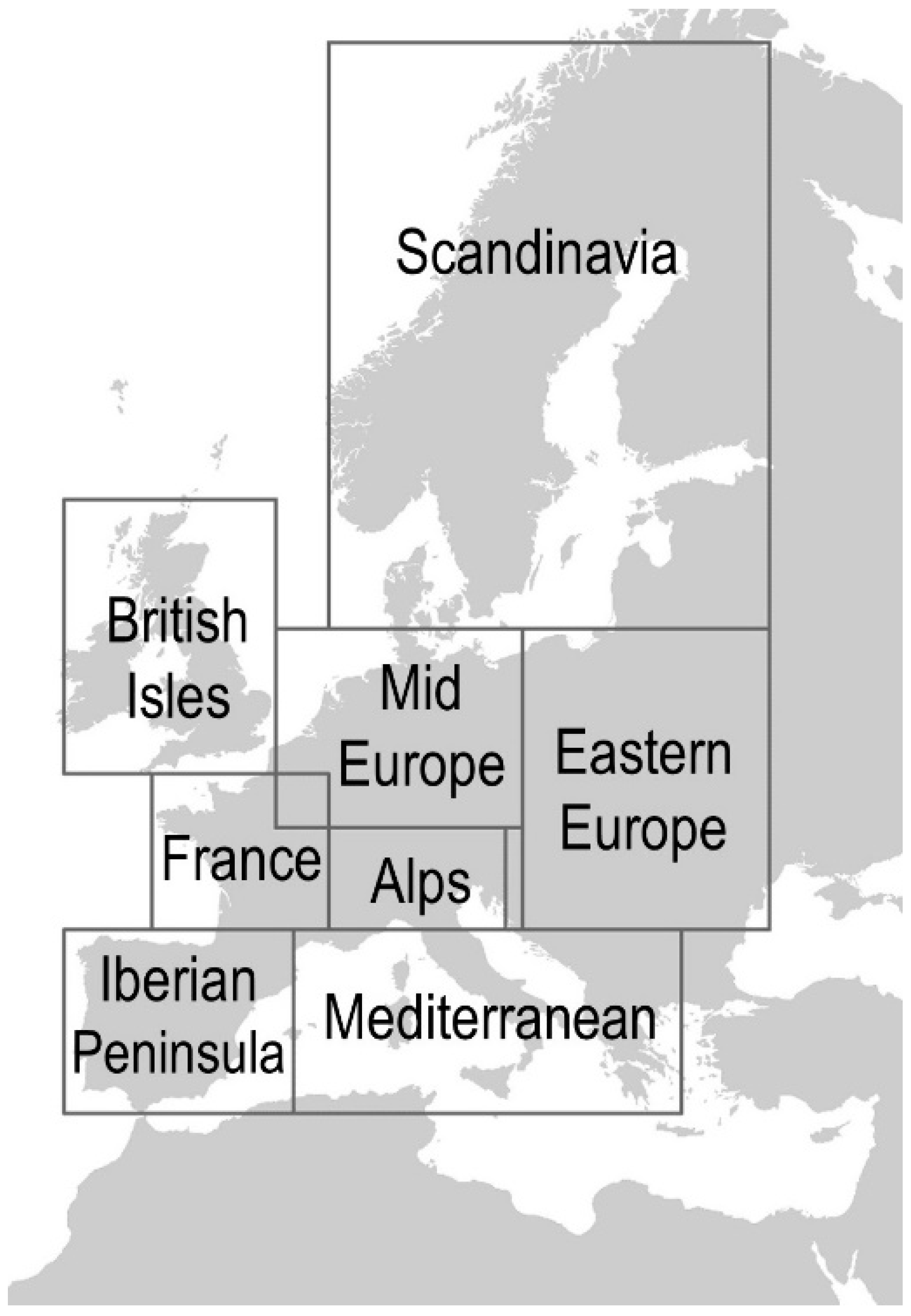
2.3. Global Warming Levels and Model Agreement

International climate policies are closely linked to warming limits [48,49]. We thus frame our analysis at specific global warming levels (GWLs) compared to the pre-industrial period, here defined as the period from 1870–1899. Spatially and temporally, monthly mean temperature from each GCM is used to define global annual mean near surface temperature resulting from RCP8.5 simulations. The year of passing a GWL is defined as the first time the 20-year running mean of the global averaged annual mean temperature is above the GWL; i.e., the year indicates the middle of a 20-year average. Future climate periods are then defined as 30-year time-slices centered on the crossing year of the corresponding GWL. The baseline period is set to 1981–2010. The models consisting of the ISIMIP, Euro-CORDEX and HELIX ensembles, along with the time that each GWL is surpassed for each model, are given in Table 2. All models reach the 1.5 °C and 2 °C warming levels, but not all of them reach the 4 °C warming level in the time frame of this study. GFDL reaches only +3.2 °C in the 2081–2100 time-slice, thus GFDL is left out of the 4 °C analysis (GFDL is a member of all three ensembles). Other models that reach warming levels of 3.75 °C and higher at the final time-slice are included in the 4 °C GWL analysis.
A number of common driving models can be identified between the three ensembles, namely: GFDL-ESM2M, HadGEM2-ES and IPSL-CM5A-LR (absent from the Euro-CORDEX ensemble). Within each ensemble, the assessment of the level of uncertainty in the projections is introduced with the percentage of the models that agree towards the climate change impact signal; i.e., the percentage of models that agree on the sign of the projected change for an examined hydrological variable. To examine whether the ensemble mean projected changes are significant compared to the inter-ensemble variability we introduce the concept of robustness in the ensemble mean projections [50]. According to this concept, the ensemble mean projected changes are considered as robust if the absolute ensemble mean change is greater than the standard deviation of the changes projected by the models that comprise the ensemble.

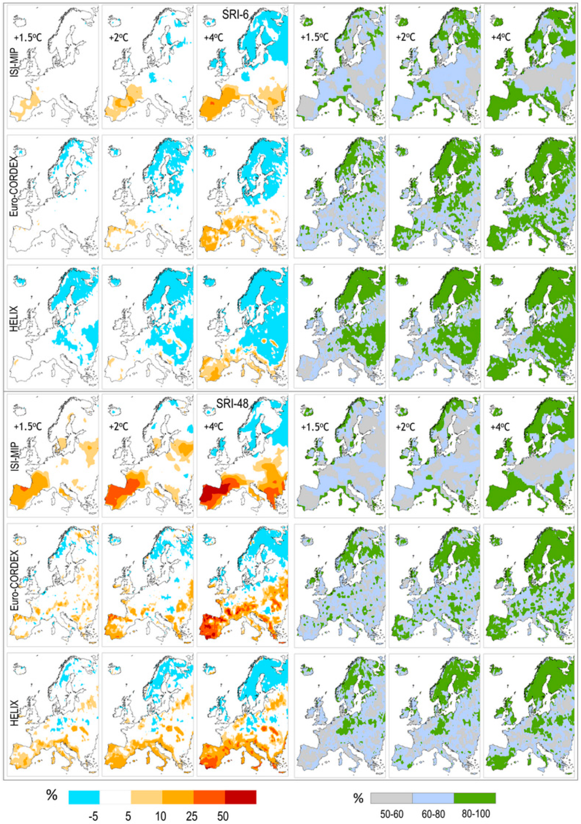
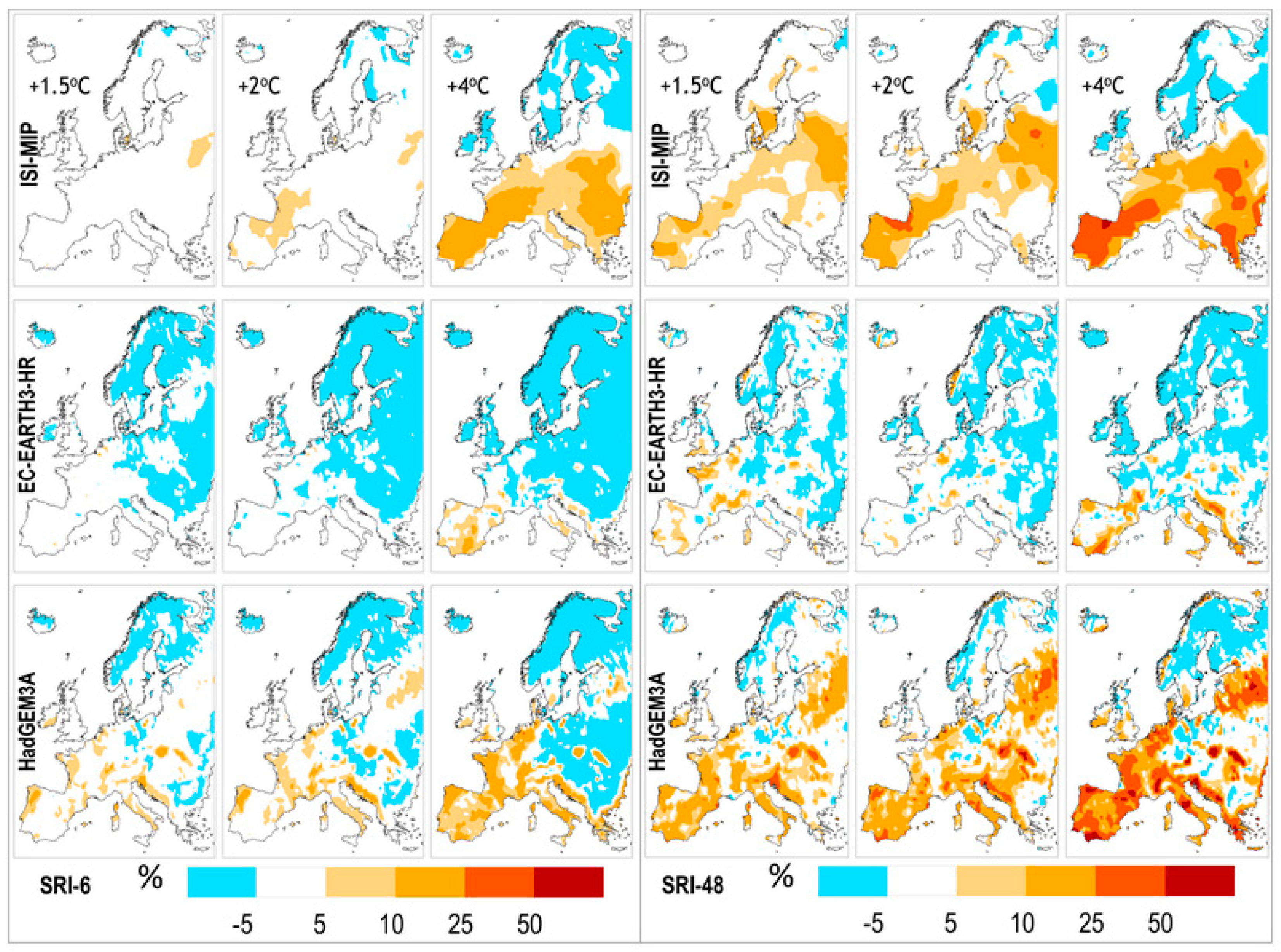
2.4. Hydrologic Indicators and Characterization of Drought

A number of hydrologic indicators are calculated from the runoff output of the JULES model, in order to express different aspects of runoff’s temporal distribution. The employed hydrologic indicators are:
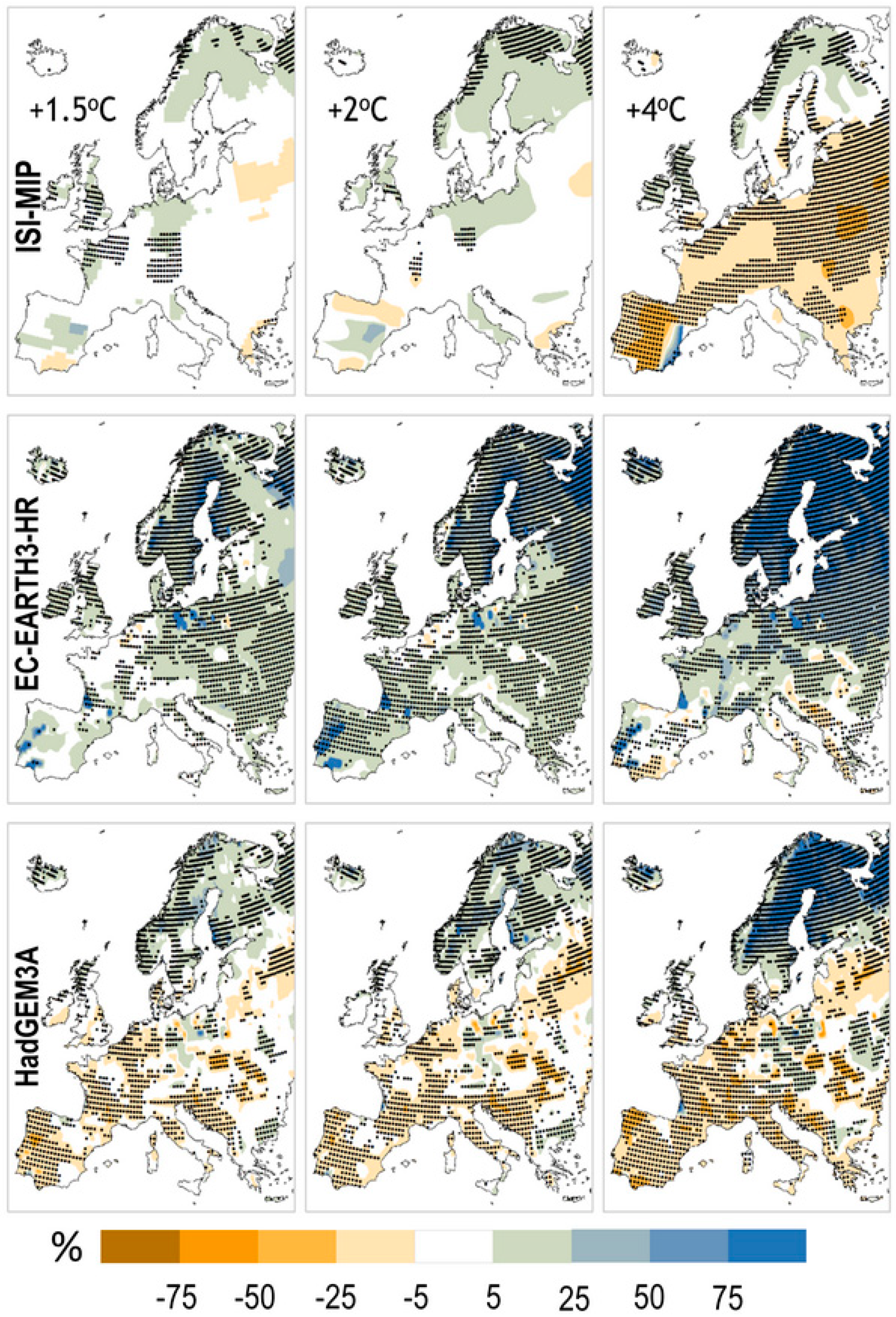
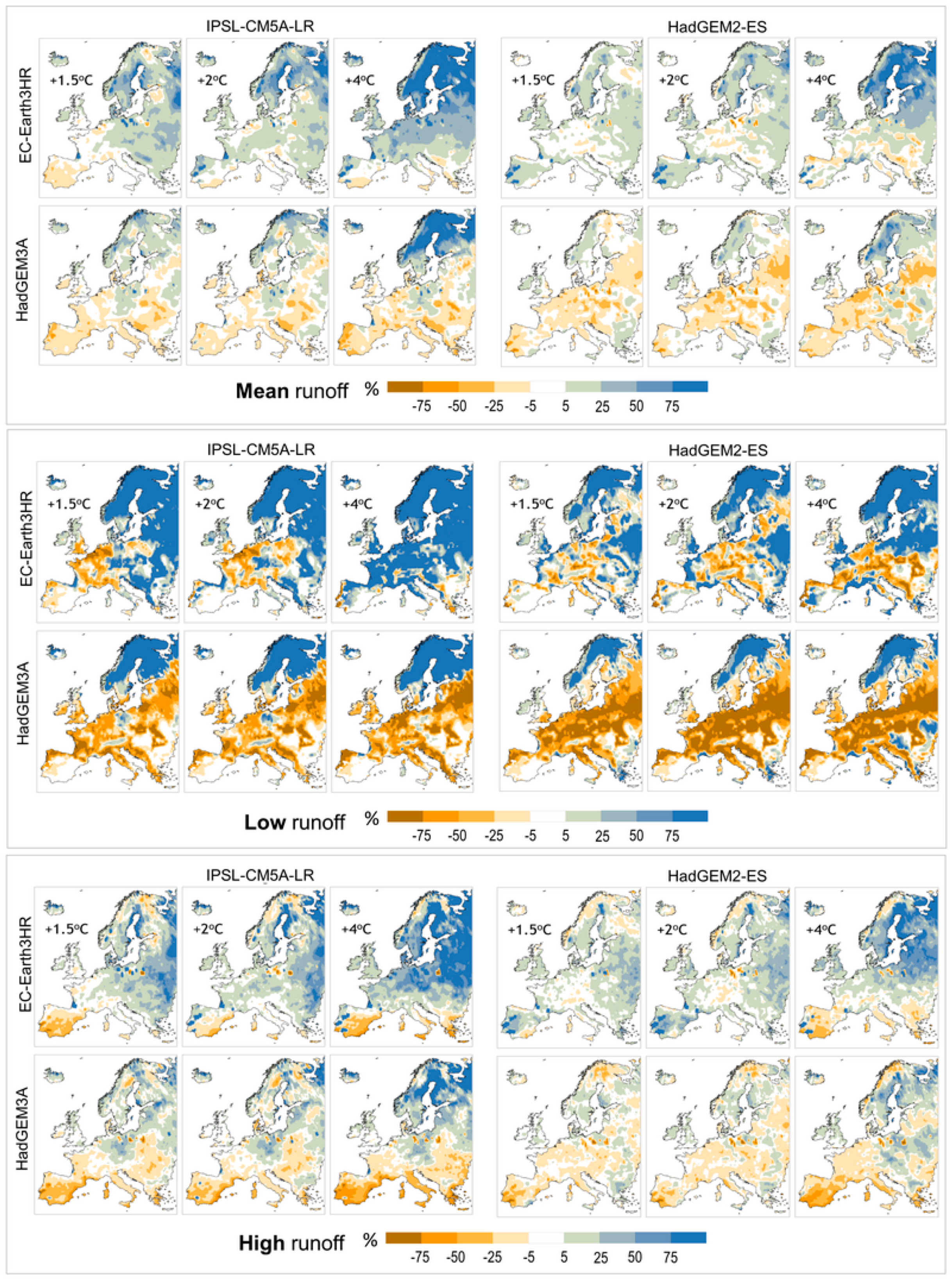
  • Mean runoff (RF mean): The long-term average of runoff is a basic indicator for mean water availability.
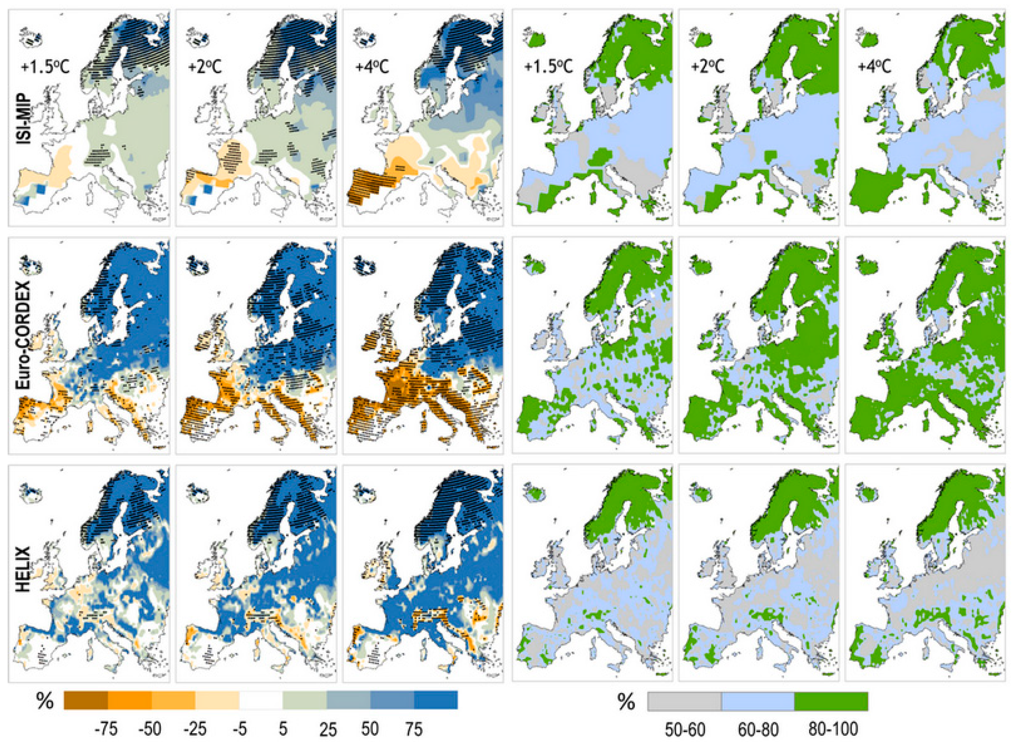
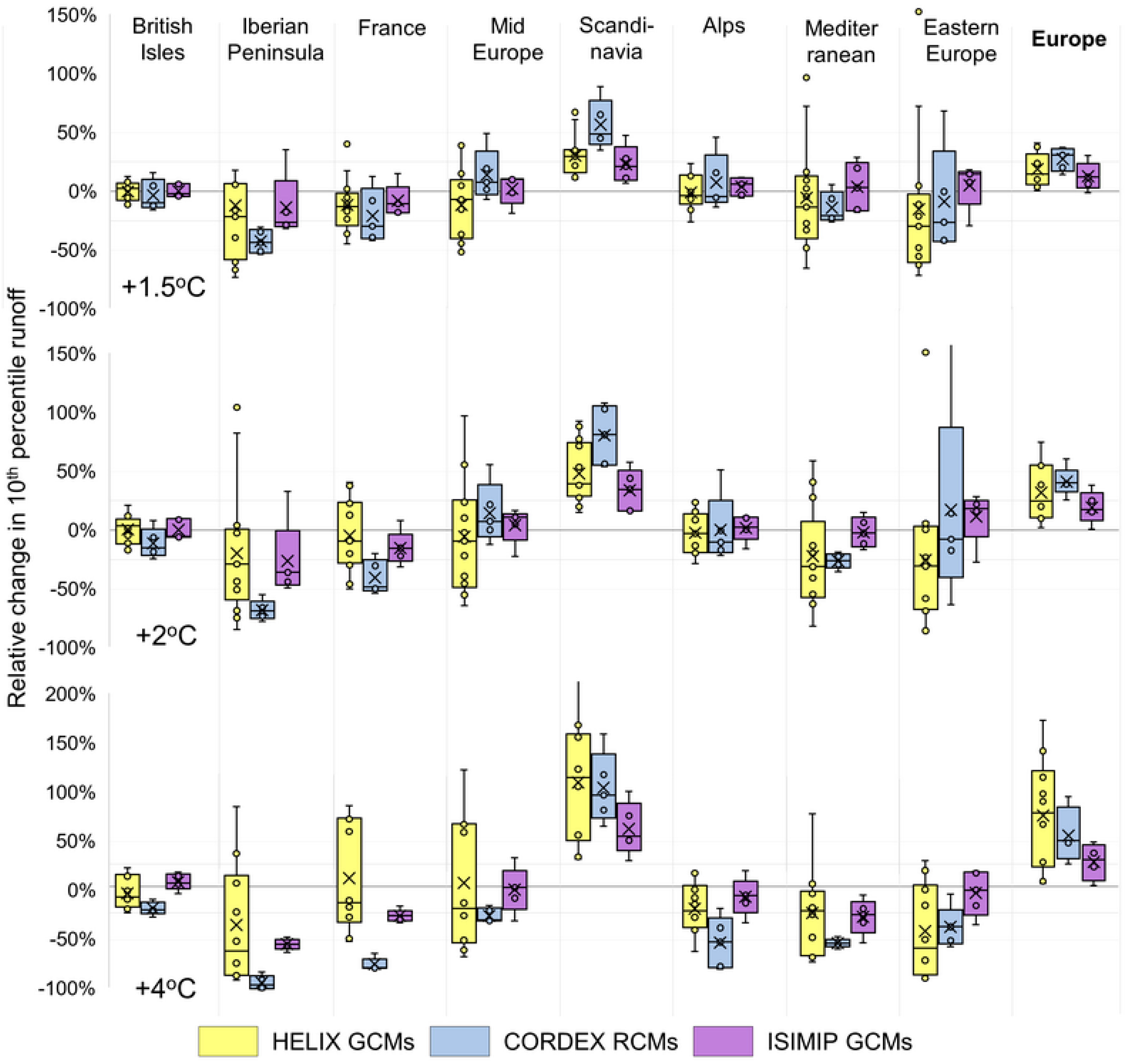
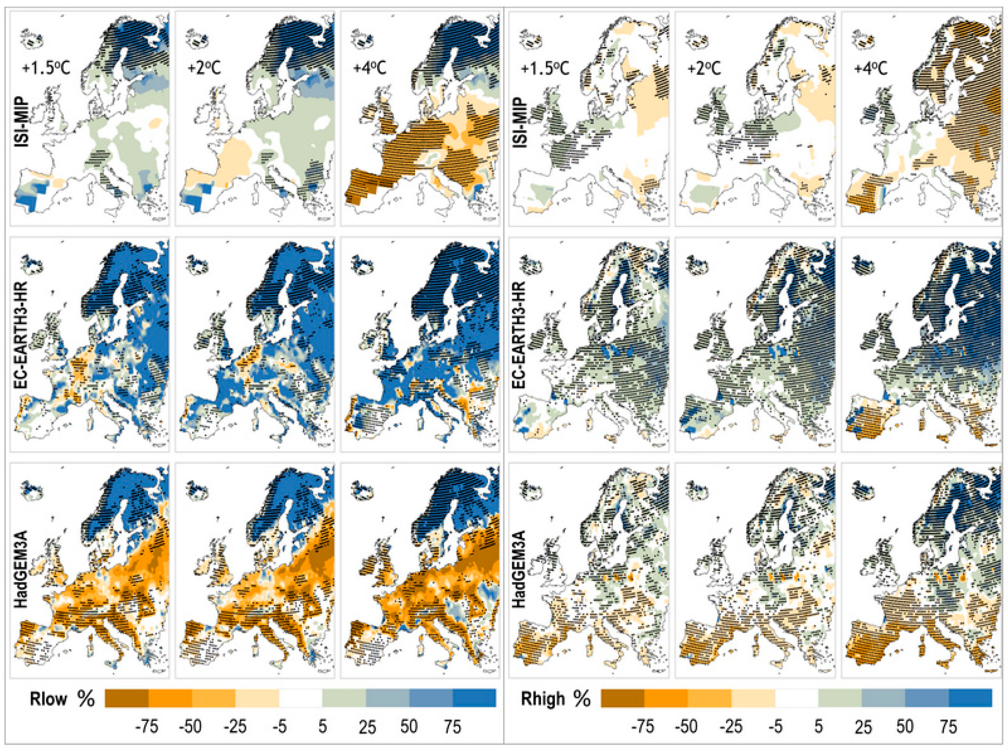
  • 10th percentile runoff (RF low): The lower 10th percentile of runoff distribution serves as an indicator for low flows.
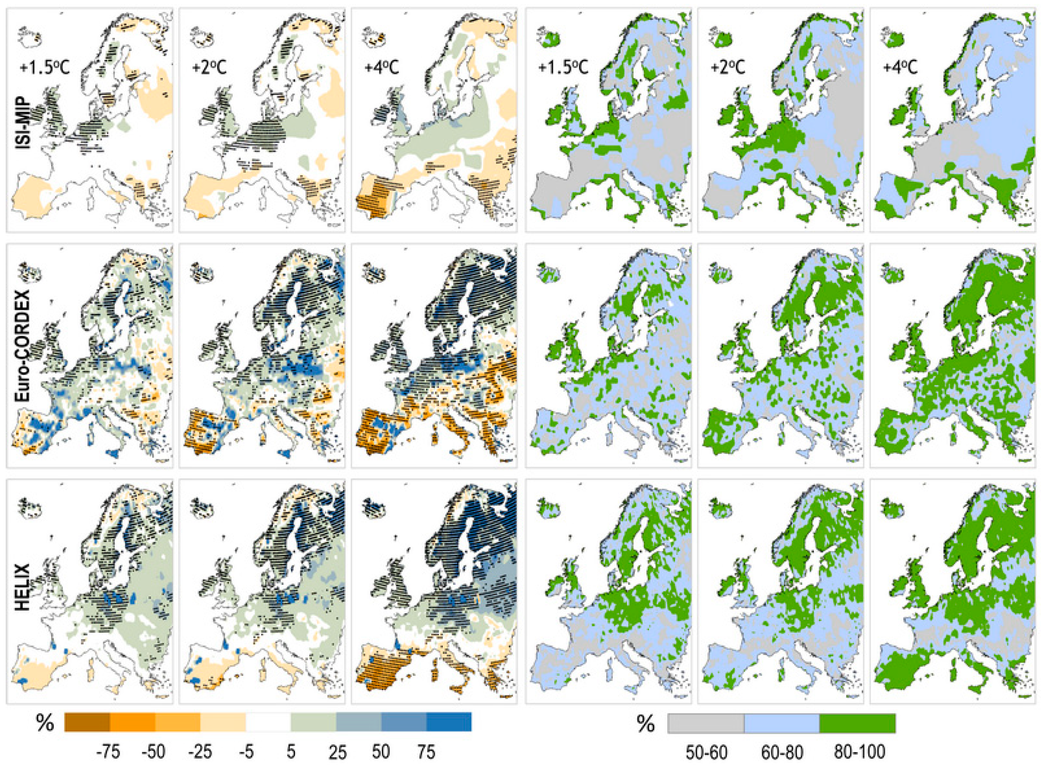
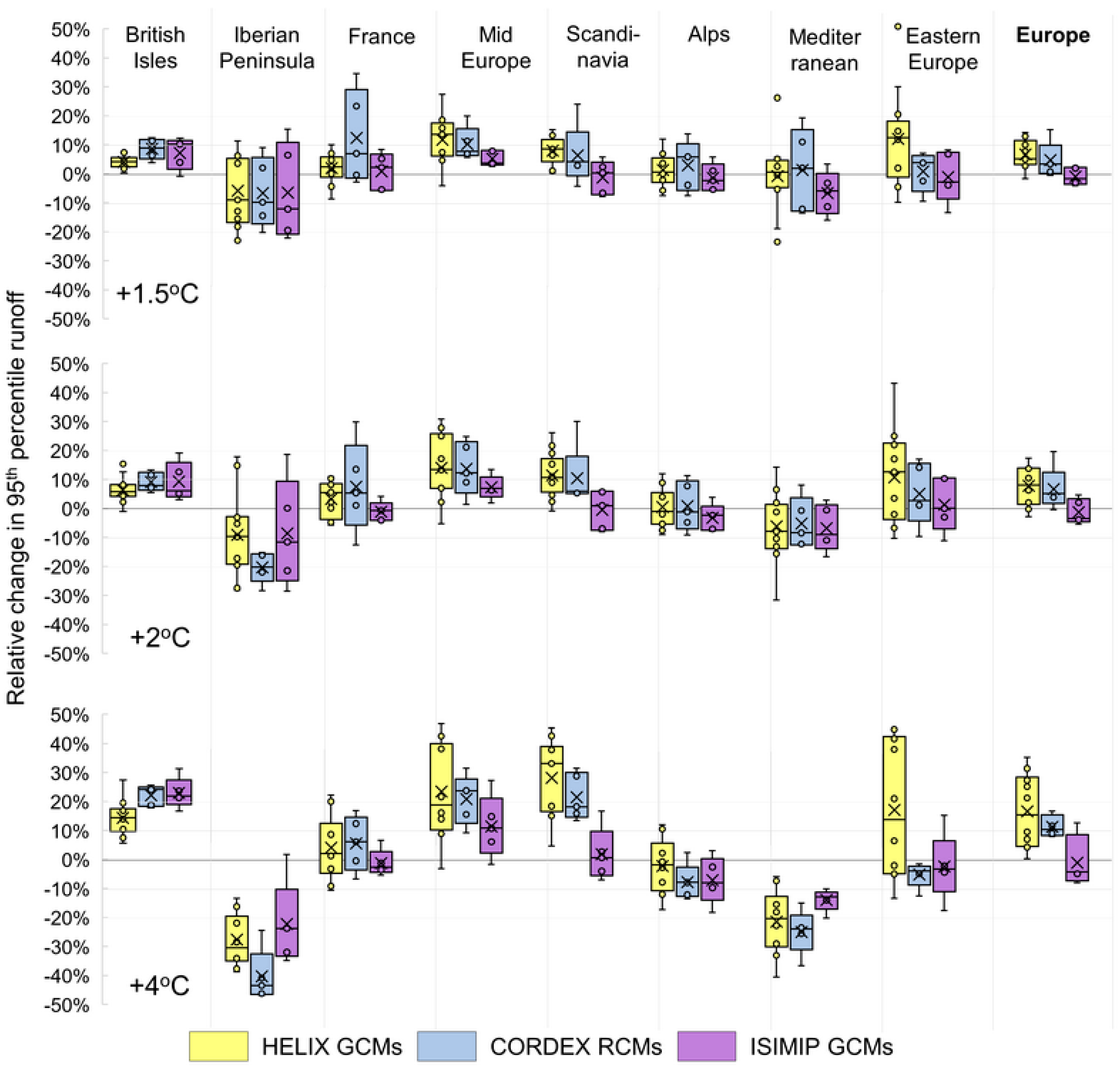
  • 95th percentile runoff (RF high): The 95th percentile of runoff distribution serves as an indicator for high flows.
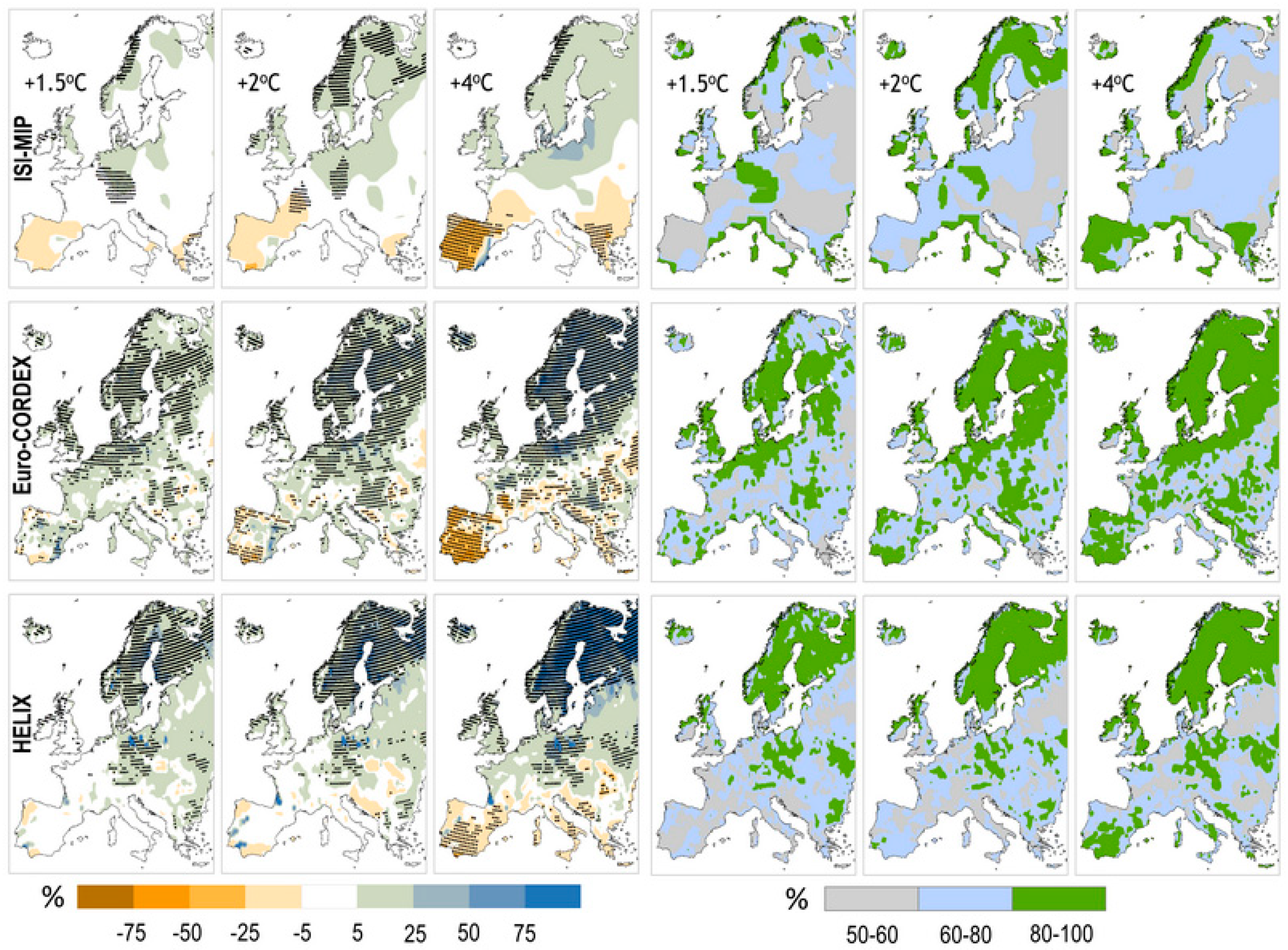
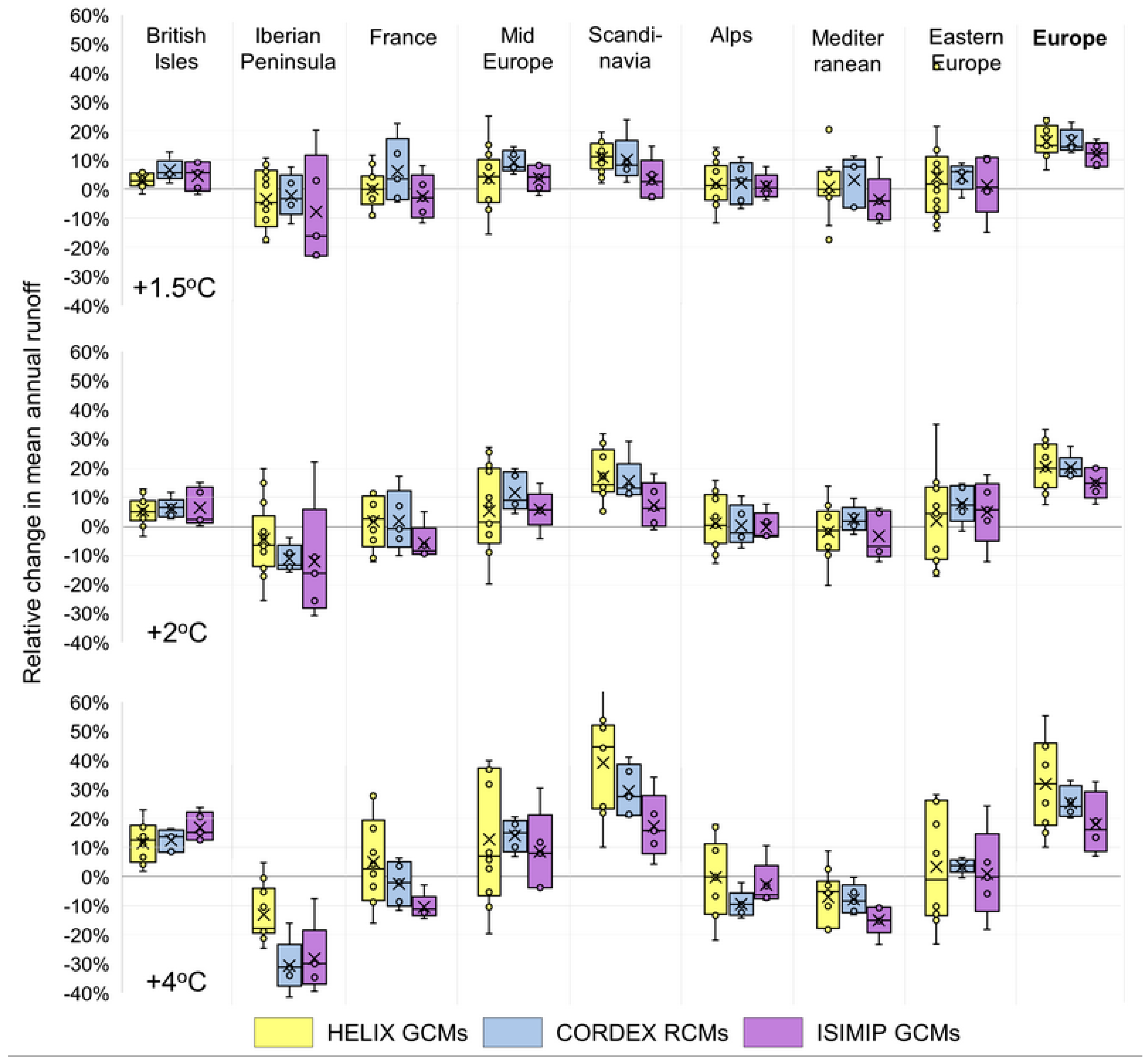
For the representation of droughts, the standardized runoff index (SRI) is employed to describe the duration and severity of hydrologic drought [51]. The index is based on the concept of the widely used standardized precipitation index (SPI [52]). Negative SRI values indicate the existence of drought conditions. According to the SRI value, drought is grouped into arbitrarily defined intensity tiers, ranging from “mild” to “extreme”. This work was focused on extreme hydrologic drought conditions, thus only values of SRI < −1.5 were considered. For the assessment of climate change impact on droughts we used the relative version of SRI [53]. Relative indices use input data of two time periods. The first period serves as the reference period and is used for model calibration. The calibrated model is then applied to data of the second time period. This allows us to assess the drought conditions of the future compared to the benchmark drought conditions of the baseline period. The relative drought indices are calculated using two periods of temporal aggregation, in order to capture droughts of different duration. A 6-month period (SRI-6) is employed for the representation of short-term events that mostly correspond to agricultural droughts and a 48-month period (SRI-48) is used to depict long-term drought events that affect the storage of water resources. Grid boxes with zero runoff for more than 90% of the length of the historical time period are excluded from the calculation of SRI.
The hydrologic indicators and time under drought conditions are derived for each time-slice. Using the reference time-slice as a baseline for comparison, their changes at different GWLs are examined on a pan-European scale, over eight large European sub-regions [54], as shown in Figure 2.

3. Results

To examine how the methodological differences of climate projection approaches affect the outputs, and hence the robustness, of the conclusions we use three different sets of projections with some common characteristics. The three sets are: a subset of five CMIP5 GCMs used in the ISIMIP; a subset of Euro-CORDEX simulations performed by one RCM with common driving models as the ISIMIP; and, a set of new high-resolution AGCM simulations also including the common driving GCMs of the first two subsets. Bias correction between the three different sets differs in terms of methods and observations used. A land surface model is used to simulate the hydrologic response of the different climate model ensembles. A number of indicators are employed to examine differences and similarities at three levels of global warming (1.5 °C, 2 °C and 4 °C). We find that these methodological differences lead to considerably different hydrologic outputs.
We further test the assumption that the regional climate changes are driven predominantly by the SSTs. We do this by looking at the hydrologic response (in terms of mean, low and high runoff) obtained by two different high-resolution AGCMs driven by the same time-varying SSTs and sea-ice concentrations (SICs).

3.1. General Comparison between Ensembles: ISIMIP vs. Euro-CORDEX vs. HELIX AGCMs

Figure 3, Figure 4, Figure 5, Figure 6, Figure 7, Figure 8 and Figure 9 compare the projected changes in hydrologic indicators and drought indices derived from the three examined ensembles (ISIMIP, Euro-CORDEX and HELIX). The projections of the three ensembles exhibit considerably different behavior. The ISIMIP projections are far less detailed than the other two, due to the lower resolution of the ISIMIP GCMs ensemble. In contrast, the Euro-CORDEX projections show more variant spatial patterns than the HELIX ensemble, although the two ensembles have a similar resolution.
A common pattern on the projected changes in mean runoff between the three ensembles (Figure 3) is the increasing signal in north and north-eastern Europe and the decreasing signal in the southern part of the continent, but with large regional uncertainties. Northern and southern Europe are regions with higher agreement on the sign of mean annual runoff change, while agreement is lower for central Europe (Figure 3).
The increasing and decreasing signals intensify and become more spatially coherent with rising warming levels. For example, the percentage of European land area with decreases (<−5%) in mean runoff expands from 10% to 23% between +1.5 °C and +4 °C for the ISIMIP ensemble, from 20% to 30% for the Euro-CORDEX ensemble and from 2% to 18% for the HELIX ensemble. At +4 °C, the three ensembles show robust decreases of mean runoff for the Mediterranean region. Meanwhile, the projected mean runoff increases over the northern part of Europe are robust regardless of the GWL, for both the Euro-CORDEX and HELIX ensembles. Spatially averaged values of relative changes in mean runoff for all the models of each ensemble and for the three examined GWLs are presented in Figure 4.
The European average shows an overall increase in mean runoff in the continent, consistently projected by the three ensembles and across GWLs. However, the model spread increases considerably when moving to GWL4, especially for the HELIX ensemble. Similar behavior to Europe is observed for the British Isles and Scandinavia. For other regions, the ensemble member values span both positive and negative changes for all the GWLs (France, Alps and Eastern Europe). For the Iberian Peninsula and the Mediterranean, the ensembles span projected increases and decreases for the lower two GWLs but agree on decreases for GWL4 (with the exception of one model of the HELIX ensemble). The model spread of the HELIX ensemble is generally larger compared to the other ensembles, especially at GWL4, which is probably due to the wider uncertainty depicted in the HELIX ensemble due to the larger number of models that are included.
Projected changes in low runoff by the ISIMIP GCMs and Euro-CORDEX ensembles show similar patterns of increased low runoff in the north and north-east and decreased low runoff in the south and south-west, although the latter ensemble projects greater changes (Figure 5).
The Euro-CORDEX projections are characterized by a robust signal over a large part of Europe, especially at GWL4. The behavior of the HELIX AGCMs ensemble is distinguished by projected increases or negligible changes in low runoff over the majority of the continent (increases over 60%, 70% and 74% of the European land area; negligible changes over 25%, 20% and 12% of the European land area, respectively for GWLs 1.5, 2 and 4). A robust signal is found only for the Scandinavian Peninsula and a small area of projected decreases in low runoff in central Europe. Concerning model agreement on the signal of low runoff projections (Figure 5), the HELIX AGCMs ensemble has the lowest extent of high model agreement (80–100%), mainly at the Scandinavian Peninsula (31% of the European land area with high model agreement at GWL4). The ISIMIP ensemble has highest agreement for the increasing changes in Scandinavian countries and the decreasing signal in the Iberian and Mediterranean while Euro-CORDEX projections highly agree (80–100% of the models) on the sign of changes in low runoff over the majority of the continent at greater GWLs (60% of the European land area under GWL4). For the regionally aggregated values, the different ensembles agree on increased low runoff for all GWLs which increases, along with model spread, for higher GWLs (Figure 6). However, Scandinavia is the only European sub-region with projected increases in low runoff by all the members of all the ensembles and across GWLs. For the rest of the regions, low runoff response to warming is a lot more complicated. For example, the British Isles and the Alps for GWLs 1.5 and 2, have a close to zero average change according to the ensemble mean, which results from a small model range, compared to other regions, between positive and negative values. For France and Mid-Europe, the spread of the Euro-CORDEX and ISIMIP ensembles decreases when moving from GWL2 to GWL4, in contrast to the HELIX ensemble which keeps a wide uncertainty range at GWL4 (from about −50% to more than 100%).
The general pattern of change for high runoff between the three ensembles, progressively more evident and intense as warming progresses, is increased high runoff in the north and north-east part of the continent and decreased high runoff in southern Europe (Figure 7). High model agreement is present only for a limited extent of the European area for the projections of the ISIMIP ensemble (25%, 28% and 25% respectively for GWLs 1.5, 2 and 4), while Euro-CORDEX and HELIX have greater areas of high model agreement at higher warming levels (22%, 35% and 58% for Euro-CORDEX, 21%, 25% and 59% for HELIX, for GWLs 1.5, 2 and 4 respectively) corresponding to the patterns of negative changes in southern Europe and positive changes in northern Europe (Figure 7). The European area aggregates show increases in high runoff projected by the HELIX and Euro-CORDEX ensembles and small (<−10%) decreases by the ISIMIP ensemble, although the individual models of the ensemble span both positive and negative values (Figure 8). The British Isles and Mid-Europe show increases in high runoff, projected consistently by the three ensembles and for the three GWLs. However, the ensemble members’ spread is larger for Mid-Europe. For the Iberian Peninsula and the Mediterranean region, the members of the three ensembles span positive and negative values of high runoff change for the lower two GWLs (with the exception of the Euro-CORDEX ensemble at +2 °C at the Iberian Peninsula only showing negative values). This mixed behavior changes to a negative signal for high runoff changes at GWL4, shown by all the members of each ensemble (with the exception of one model of the ISIMIP ensemble for the Iberian Peninsula that shows a marginally positive value of change).
The comparison of the projected changes in hydrologic indicators of the three examined ensembles reveals remarkably diverse patterns between the ensembles. A greater similarity can be observed between the spatial patterns of projected changes in extreme drought duration of the three ensembles. For short-term droughts (modeled with SRI6), all the ensembles project increases in drought duration in the Mediterranean region at GWL4, while only the ISIMIP shows spatially coherent regions of increased drought duration at lower levels of warming (increases over 5% and 9% of the European land area for GWL1.5 and 2 respectively, compared to 1% and 4% for Euro-CORDEX, and 1% and 3% for HELIX) (Figure 9). Especially at GWL4, the regions of increased drought duration are also regions with high model agreement on the sign of the change of short-term drought duration. The projected changes in time under long-term extreme drought conditions (modeled with SPI48) are more intense and spatially extended compared to short-term droughts, with projected increases at GWL4 covering 32%, 35% and 32% of the European land area for the ISIMIP, Euro-CORDEX and HELIX ensembles respectively. Again, similar patterns can be found between the three ensembles. Under +4 °C of warming, increased drought duration is projected for southern Europe by all the ensembles. The agreement of the models is less uniform between the three ensembles. At GWL4, the ISIMIP ensemble exhibits high agreement over the whole south-European region, Euro-CORDEX shows patches of high agreement all over southern Europe while the HELIX AGCMs ensemble shows high agreement on increased drought duration only for the southern Iberian Peninsula, Sardinia and southern Italy. However, the fraction of European land area with high agreement on the sign of projected changes in extreme long-term drought duration is similar between the three ensembles (55%, 49% and 45% at GWL4, for the ISIMIP, Euro-CORDEX and HELIX ensembles respectively).

3.2. The Effect of the High-Resolution AGCM

The results of this section (Figure 10, Figure 11 and Figure 12) show the differences in projected changes caused by the two high-resolution HELIX AGCMs, as only the ensemble members forced with common driving models participate here (GFDL-ESM2M, IPSL-CM5A-LR and HadGEM2-ES). For all runoff metrics, mean (Figure 10) and low and high (Figure 11) runoff, very different patterns of change can be observed between the two HELIX AGCMs.
EC-EARTH3-HR projects a considerably wetter future, with increases in hydrologic indicators of mean, low and high runoff over most of the European area (80%, 78% and 72% at GWL4, for mean, low and high runoff respectively). In contrast, negative changes are projected by HadGEM3A, especially for low runoff, for the greater part of Europe (42%, 54% and 38% at GWL4 for mean, low and high runoff respectively). This indicates that the atmosphere model used for the production of climate simulation plays a vital role in the signal of the projected impacts and designates the selection of the HELIX model as a major source of uncertainty for the projected simulations. It can be observed that the ISIMIP sub-ensemble resembles the signal of the HadGEM3A sub-ensemble. This could possibly indicate that HadGEM3A preserved the signal of the original GCMs that were used as its forcing, while the processes within EC-EARTH3-HR resulted in a shift of the original GCM climate signal.
Figure 12 shows the changes in short- and long-term drought respectively, as simulated by the three sub-ensembles. Again, it can be observed that the ISIMIP patterns are closer to those of HadGEM3A. EC-EARTH3-HR projects a small and spatially incoherent increase in drought duration at the pan-European level (0%, 1% and 8% of the European land area for GWLs 1.5, 2 and 4 regarding short-term droughts; 11%, 6% and 13% for long-term droughts). In contrast, the ISIMIP and HadGEM3A show increased drought duration for a large proportion of the continent, covering almost all of southern and central Europe, especially at GWL4 (41% and 29% for ISMIP and HadGEM3A respectively regarding short-term droughts; 45% and 47% for long-term droughts), and with alarming values of increase in duration (>50%) for long-term droughts.

3.3. The Response of Atmosphere Models on the Drier (r1) and Wetter (r3) Forcing

To further investigate how the atmosphere models and forcing models affect the projected changes in runoff indicators, we compare single ensemble members forced with the same driving model and different atmosphere models. This comparison is performed for the drier and warmer (r1-IPSL-CM5A-LR [55]) and wetter (r3-HadGEM2-ES) of the common driving models, in order to account for the widest range of uncertainty. Figure 13 shows the changes in mean, low and high runoff when the two high-resolution atmosphere models (EC-Earth3-HR and HadGEM3A) are forced with r1 and r3 respectively. A visual comparison of the figures for mean, low and high runoff reveals that there is a higher resemblance between the changes forced by the same atmosphere model than with the same driving model. Simulations of the same driving model, whether this is the wetter or the drier, have very different spatial patterns and different signal of change for the same regions. On the contrary, the differences are far less pronounced for the simulations that use the same atmosphere model, although they use a different driving model (r1 or r3).

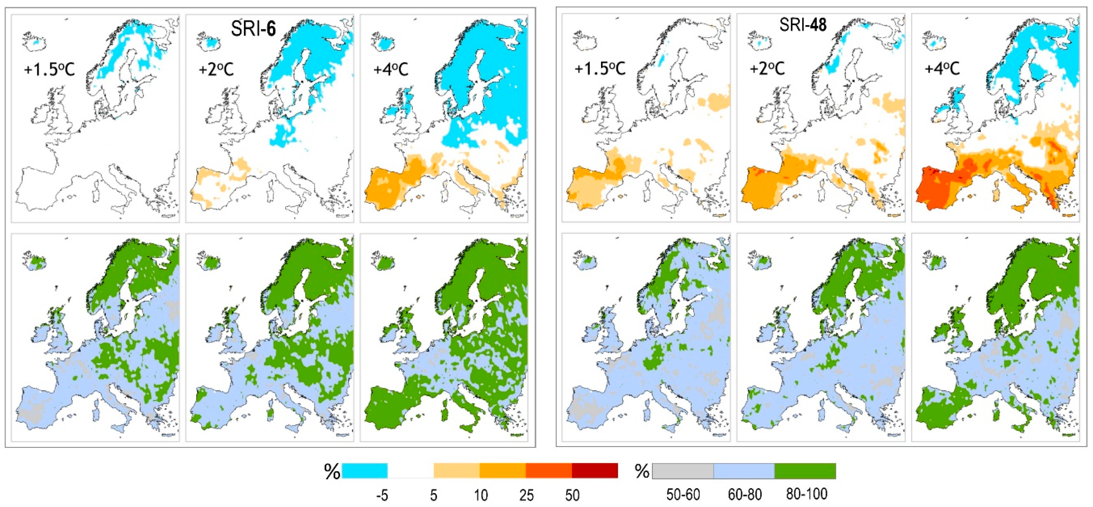
3.4. A combined Ensemble, Consisting of the Three Subsets (for SRI)

So far, we have examined differences in the projected changes in runoff indicators and duration of drought conditions derived by three different ensembles. Here we combine the three ensembles (ISIMIP, EURO-CORDEX and HELIX) into one, and examine the projected changes in short- and long-term drought conditions (Figure 14), along with the model agreement of the extended ensemble on the sign of change of drought duration.
The combined ensemble shows virtually no increases in short-term drought duration at GWL1.5, small increases in short-term drought duration over regions of the Iberia Peninsula at GWL2, and increases ranging from 5 to 25% for the Mediterranean region at GWL4 (Figure 14). Increased drought duration affects only 4% of the European land area at GWL2, but this area considerably expands to cover 18% of the continent at GWL4. It is important to note that the aforementioned regions of drought duration increases in the Mediterranean also show a high level of model agreement.
Regarding long-term droughts, the combined ensemble shows increases of 5 to 25% in duration over the Iberian Peninsula, western France, Italy and Greece at GWLs 1.5 and 2 (increases affect 17% and 22% of the European land area at GWLs 1.5 and 2 respectively). However, the confidence on these changes is debatable, as only 60–80% of the combined ensemble members agree on the sign of the changes. At GWL4, the combined ensemble shows increases in long-term drought conditions of up to 50%, affecting all the southern part of Europe and even regions of central Europe (increased drought duration over 38% of the land surface). Nonetheless, regions of high agreement (80–100%) on these changes are only the Mediterranean regions.

4. Discussion and Conclusions

Here we assessed higher resolution hydrological projections under high-end climate change (RCP8.5) in Europe as simulated by the JULES land surface model (LSM). We compared a set of new high-resolution AGCM projections (HELIX) with previous assessments based on the same LSM and climate data of coarser spatial resolutions and fewer ensemble members (ISIMIP and Euro-CORDEX). For the HELIX ensemble, we chose models with higher resolution than the CMIP5 models to benefit from the advantages of higher resolution. The projections were examined for three levels of global warming (+1.5 °C, +2 °C and +4 °C), as relative changes compared to a reference period of the recent past (1981–2010). Through a number of comparisons between the changes in hydrologic indicators and drought conditions projected by the different ensembles and their members, we explored:
  • the differences and similarities between the projections of the three ensembles and assessed the possible added value provided by the newer HELIX AGCMs simulations.
  • the effect of the HELIX AGCM on the projections as simulated by the JULES LSM.
  • the impact of the +4GWL compared to the +2GWL and +1.5GWL.
The comparison of the different model ensembles revealed large differences in the projected hydrological impacts, with conflicting signs of change for some runoff metrics. In summary, the highest level of consensus between the ensembles was observed for changes in mean runoff. The climate change signal for mean runoff showed increases in the north of Europe, decreases in the south and only small changes with lower model agreement for central Europe. For low runoff, the HELIX ensemble showed increased response over most of Europe, but also exhibited low model agreement on the sign of change for most of the European area. The other two ensembles showed a different response of low runoff to climate change, as both agreed on increased low runoff in the north-eastern part of Europe and decreased low runoff over the south-western part of the continent. Regarding changes in high runoff, all three ensembles showed negative changes for the southern part of Europe but had different signals for central Europe. The three examined ensembles show a markedly more similar response regarding the drought duration projections. For short-term droughts, all the ensembles showed increased drought duration over the Mediterranean, while for long-term droughts the region of increased drought duration extended to the whole of southern Europe. Moreover, the projected increase in drought duration was larger for long-term compared to short-term droughts.
Examination of the role of the high-resolution atmosphere model for the hydrological simulations revealed that the two AGCMs projected very different futures of conflicting climate change signals. Specifically, HadGEM3A projected a dramatically drier future, while EC-EARTH3-HR projected a wetter future in terms of runoff production metrics. This could be attributed to the warm biases of the HadGEM3A [31]. Regarding the drought analysis, HadGEM3A showed increased drought duration for a considerably larger part of Europe compared to EC-EARTH3-HR. The projected climate change signal was determined by the atmosphere model rather than by the SSTs driving model. The combined ensemble showed that spatially coherent regions of increased drought duration and high model agreement appear under +4 °C of warming over the Mediterranean region.
Earlier studies have shown that increases in GCM resolution improve the simulation of extreme precipitation and drought events, due to a better depiction of sub-seasonal, synoptic and mesoscale variability by the models [56,57,58]. Here, the higher resolution ensemble showed a greater spread of results compared to the other ensembles. First, this might be a consequence of the larger number of models participating in the ensemble. Second, an increase in the range of the results in the ensemble does not necessarily point towards an increase of the uncertainty. Instead, it can possibly be attributed to the increase in spatial detail of the projections, which, even though it has the advantage of improved projections, might result in erroneous information after averaging of the high-resolution outcomes to less detailed spatial scales, as the expressed spatial variability is lost.
In the context of the present study, interpretation of the impact of high-resolution climate data on hydrological projections should take into account that results have been based on a single hydrological model. The JULES model, in contrast to most hydrological models, includes the representation of plant stomatal closure to elevated CO2 concentrations which causes evaporation to reduce, and thus climate impacts on runoff production to appear less pronounced [48]. Such differences in the structure and assumptions of the models, lead to considerable uncertainty relating to the choice of the impact model [59,60,61], especially when analysis focuses on hydrological extremes [21]. For this reason many studies have pointed out the need for multi-impact model assessments to capture the impact model induced uncertainty in the projections [62,63,64]. However, single model studies can still provide useful conclusions and indications on matters that need to be further investigated in more complex and computationally demanding multi-model assessments [8].
Our study underlines the need for biophysical impact modelers to be particularly meticulous in their analysis when it involves handling a subset of climate models. A first point on which extra care should be taken is the treatment of outputs. Our findings indicate that in many cases, the ensemble mean of a set of climate projections might not be a good representative of the projected changes, as ensemble members’ values might span both positive and negative values. In these cases, the variability of the projections is lost to a close to zero value of the ensemble mean. Moreover, the spatiotemporal aggregation over large domains or at country level that is typically used to communicate changes should be critically used and discussed, as it might cause loss of the benefits of higher resolution simulations. A second point that requires attention when interpreting results on impacts concerns the time-slices employed, especially when they are based on levels of warming. The different timing of crossing a specific warming level between the ensemble members has a direct impact on the results. The radiative forcing is evolving with time (depending on the emission scenario) and is different for each member depending on the time of crossing the GWLs of the driving GCM. When comparing the different ensembles, the different timing of GWLs between them, due to the different models and/or different number of models in the ensemble, might impose an extra source of uncertainty on the results. A third point requiring extra care when dealing with impacts at the regional scale is the selection of available RCM simulations. For many RCM domains, there is generally an imbalance in the number of available downscaling simulations. For some regional climate change assessment programs, the majority of simulations are conducted from a single RCM and a limited number of simulations by different RCMs complement the ensemble of available future climate projections. The disparity in available simulations might cause a bias of the projected impacts towards a specific climate model.
In general, the assumptions and choices made during the design of an impact study can have a crucial effect on the documented results. Selection of the climate models that comprise an ensemble for a specific study should be made after scrutiny and investigation of the range and differences of parameters relevant to the simulations of impacts of interest, and not solely on precipitation and temperature. Finally, uncertainty is an unavoidable part of climate and impact modeling in any given context, so transparent assessment and proper communication of uncertainty can improve the quality of research outputs provided to policymakers, and thus help to inform adaptation relevant policy decisions under a changing climate.

Author Contributions

Conceptualization and methodology, A.G.K. and L.V.P.; software (climate model simulations), K.W., J.C. and R.A.B.; formal analysis and investigation, A.G.K. and L.V.P.; resources and data curation, M.G.G., K.W. and J.C.; writing-original draft preparation, A.G.K. and L.V.P.; writing-review and editing, all authors; visualization, A.G.K. and L.V.P.; project administration, I.K.T. and R.A.B.; funding acquisition, I.K.T. and R.A.B.

Funding

The research leading to these results has received funding from the European Union Seventh Framework Programme FP7/2007-2013 under Grant Agreement No. 603,864 (HELIX: High-End cLimate Impacts and eXtremes; www.helixclimate.eu).

Acknowledgments

The EC-EARTH3-HR simulations were performed on resources provided by the Swedish National Infrastructure for Computing (SNIC) at PDC and the HadGEM3 simulations were performed at the Met Office Hadley Centre.

Conflicts of Interest

The authors declare no conflicts of interest.

References

  1. Lutz, A.F.; Ter Maat, H.W.; Biemans, H.; Shrestha, A.B.; Wester, P.; Immerzeel, W.W. Selecting representative climate models for climate change impact studies: An advanced envelope-based selection approach. Int. J. Climatol. 2016, 36, 3988–4005. [Google Scholar] [CrossRef]
  2. Mendlik, T.; Gobiet, A. Selecting climate simulations for impact studies based on multivariate patterns of climate change. Clim. Chang. 2016, 135, 381–393. [Google Scholar] [CrossRef] [PubMed]
  3. McSweeney, C.F.; Jones, R.G.; Lee, R.W.; Rowell, D.P. Selecting CMIP5 GCMs for downscaling over multiple regions. Clim. Dyn. 2015, 44, 3237–3260. [Google Scholar] [CrossRef]
  4. Sun, Q.; Miao, C.; Duan, Q. Comparative analysis of CMIP3 and CMIP5 global climate models for simulating the daily mean, maximum, and minimum temperatures and daily precipitation over China. J. Geophys. Res. Atmos. 2015, 120. [Google Scholar] [CrossRef]
  5. Nikulin, G.; Asharaf, S.; Magariño, M.E.; Calmanti, S.; Cardoso, R.M.; Bhend, J.; Fernández, J.; Frías, M.D.; Fröhlich, K.; Früh, B.; et al. Dynamical and statistical downscaling of a global seasonal hindcast in eastern Africa. Clim. Serv. 2017. [Google Scholar] [CrossRef]
  6. Ramarohetra, J.; Pohl, B.; Sultan, B. Errors and uncertainties introduced by a regional climate model in climate impact assessments: Example of crop yield simulations in West Africa. Environ. Res. Lett. 2015, 10, 124014. [Google Scholar] [CrossRef] [Green Version]
  7. Grillakis, M.G.; Koutroulis, A.G.; Daliakopoulos, I.N.; Tsanis, I.K. A method to preserve trends in quantile mapping bias correction of climate modeled temperature. Earth Syst. Dyn. 2017, 8, 889–900. [Google Scholar] [CrossRef] [Green Version]
  8. Papadimitriou, L.V.; Koutroulis, A.G.; Grillakis, M.G.; Tsanis, I.K. The effect of GCM biases on global runoff simulations of a land surface model. Hydrol. Earth Syst. Sci. 2017, 21, 4379–4401. [Google Scholar] [CrossRef] [Green Version]
  9. Hagemann, S.; Chen, C.; Haerter, J.O.; Heinke, J.; Gerten, D.; Piani, C. Impact of a Statistical Bias Correction on the Projected Hydrological Changes Obtained from Three GCMs and Two Hydrology Models. J. Hydrometeorol. 2011, 12, 556–578. [Google Scholar] [CrossRef]
  10. Koutroulis, A.G.; Grillakis, M.G.; Daliakopoulos, I.N.; Tsanis, I.K.; Jacob, D. Cross sectoral impacts on water availability at +2 °C and +3 °C for east Mediterranean island states: The case of Crete. J. Hydrol. 2016, 532. [Google Scholar] [CrossRef]
  11. Koutroulis, A.G.; Tsanis, I.K.; Daliakopoulos, I.N.; Jacob, D. Impact of climate change on water resources status: A case study for Crete Island, Greece. J. Hydrol. 2013, 479, 146–158. [Google Scholar] [CrossRef] [Green Version]
  12. Madsen, M.S.; Langen, P.L.; Boberg, F.; Christensen, J.H. Inflated Uncertainty in Multimodel-Based Regional Climate Projections. Geophys. Res. Lett. 2017, 44, 11606–11613. [Google Scholar] [CrossRef] [PubMed]
  13. Graham, L.P.; Hagemann, S.; Jaun, S.; Beniston, M. On interpreting hydrological change from regional climate models. Clim. Chang. 2007, 81, 97–122. [Google Scholar] [CrossRef] [Green Version]
  14. Karlsson, I.B.; Sonnenborg, T.O.; Refsgaard, J.C.; Trolle, D.; Børgesen, C.D.; Olesen, J.E.; Jeppesen, E.; Jensen, K.H. Combined effects of climate models, hydrological model structures and land use scenarios on hydrological impacts of climate change. J. Hydrol. 2016, 535, 301–317. [Google Scholar] [CrossRef]
  15. Grillakis, M.G.; Koutroulis, A.G.; Tsanis, I.K. Climate change impact on the hydrology of Spencer Creek watershed in Southern Ontario, Canada. J. Hydrol. 2011, 409. [Google Scholar] [CrossRef]
  16. Fang, G.; Yang, J.; Chen, Y.; Li, Z.; De Maeyer, P. Impact of GCM structure uncertainty on hydrological processes in an arid area of China. Hydrol. Res. 2017. [Google Scholar] [CrossRef]
  17. Mendoza, P.A.; Clark, M.P.; Mizukami, N.; Gutmann, E.D.; Arnold, J.R.; Brekke, L.D.; Rajagopalan, B. How do hydrologic modeling decisions affect the portrayal of climate change impacts? Hydrol. Process. 2016, 30, 1071–1095. [Google Scholar] [CrossRef]
  18. Taylor, K.E.; Stouffer, R.J.; Meehl, G.A. An Overview of CMIP5 and the Experiment Design. Bull. Am. Meteorol. Soc. 2012, 93, 485–498. [Google Scholar] [CrossRef] [Green Version]
  19. McSweeney, C.F.; Jones, R.G. How representative is the spread of climate projections from the 5 CMIP5 GCMs used in ISI-MIP? Clim. Serv. 2016, 1, 24–29. [Google Scholar] [CrossRef]
  20. Warszawski, L.; Frieler, K.; Huber, V.; Piontek, F.; Serdeczny, O.; Schewe, J. The Inter-Sectoral Impact Model Intercomparison Project (ISI-MIP): Project framework. Proc. Natl. Acad. Sci. USA 2014, 111, 3228–3232. [Google Scholar] [CrossRef] [PubMed]
  21. Prudhomme, C.; Giuntoli, I.; Robinson, E.L.; Clark, D.B.; Arnell, N.W.; Dankers, R.; Fekete, B.M.; Franssen, W.; Gerten, D.; Gosling, S.N.; et al. Hydrological droughts in the 21st century, hotspots and uncertainties from a global multimodel ensemble experiment. Proc. Natl. Acad. Sci. USA 2014, 111, 3262–3267. [Google Scholar] [CrossRef] [PubMed] [Green Version]
  22. Van Vliet, M.T.H.; Donnelly, C.; Strömbäck, L.; Capell, R.; Ludwig, F. European scale climate information services for water use sectors. J. Hydrol. 2015, 528, 503–513. [Google Scholar] [CrossRef]
  23. Rummukainen, M. Added value in regional climate modeling. Wiley Interdiscip. Rev. Clim. Chang. 2016, 7, 145–159. [Google Scholar] [CrossRef]
  24. Jacob, D.; Petersen, J.; Eggert, B.; Alias, A.; Christensen, O.B.; Bouwer, L.M.; Braun, A.; Colette, A.; Déqué, M.; Georgievski, G.; et al. EURO-CORDEX: New high-resolution climate change projections for European impact research. Reg. Environ. Chang. 2014, 14, 563–578. [Google Scholar] [CrossRef]
  25. Caron, L.-P.; Jones, C.G.; Winger, K. Impact of resolution and downscaling technique in simulating recent Atlantic tropical cylone activity. Clim. Dyn. 2011, 37, 869–892. [Google Scholar] [CrossRef]
  26. Manganello, J.V.; Hodges, K.I.; Kinter, J.L.; Cash, B.A.; Marx, L.; Jung, T.; Achuthavarier, D.; Adams, J.M.; Altshuler, E.L.; Huang, B.; et al. Tropical Cyclone Climatology in a 10-km Global Atmospheric GCM: Toward Weather-Resolving Climate Modeling. J. Clim. 2012, 25, 3867–3893. [Google Scholar] [CrossRef]
  27. Koutroulis, A.G.; Grillakis, M.G.; Tsanis, I.K.; Papadimitriou, L. Evaluation of precipitation and temperature simulation performance of the CMIP3 and CMIP5 historical experiments. Clim. Dyn. 2016, 47. [Google Scholar] [CrossRef]
  28. de Souza Custodio, M.; da Rocha, R.P.; Ambrizzi, T.; Vidale, P.L.; Demory, M.-E. Impact of increased horizontal resolution in coupled and atmosphere-only models of the HadGEM1 family upon the climate patterns of South America. Clim. Dyn. 2017, 48, 3341–3364. [Google Scholar] [CrossRef]
  29. Zhang, L.; Wu, P.; Zhou, T.; Roberts, M.J.; Schiemann, R. Added value of high resolution models in simulating global precipitation characteristics. Atmos. Sci. Lett. 2016, 17, 646–657. [Google Scholar] [CrossRef] [Green Version]
  30. Hewitt, H.T.; Copsey, D.; Culverwell, I.D.; Harris, C.M.; Hill, R.S.R.; Keen, A.B.; McLaren, A.J.; Hunke, E.C. Design and implementation of the infrastructure of HadGEM3: The next-generation Met Office climate modelling system. Geosci. Model Dev. 2011, 4, 223–253. [Google Scholar] [CrossRef]
  31. Vautard, R.; Christidis, N.; Ciavarella, A.; Alvarez-Castro, C.; Bellprat, O.; Christiansen, B.; Colfescu, I.; Cowan, T.; Doblas-Reyes, F.; Eden, J.; et al. Evaluation of the HadGEM3-A simulations in view of detection and attribution of human influence on extreme events in Europe. Clim. Dyn. 2018, 1–24. [Google Scholar] [CrossRef] [Green Version]
  32. Hazeleger, W.; Wang, X.; Severijns, C.; Ştefănescu, S.; Bintanja, R.; Sterl, A.; Wyser, K.; Semmler, T.; Yang, S.; van den Hurk, B.; et al. EC-Earth V2.2: Description and validation of a new seamless earth system prediction model. Clim. Dyn. 2011, 39, 2611–2629. [Google Scholar] [CrossRef]
  33. Hempel, S.; Frieler, K.; Warszawski, L.; Schewe, J.; Piontek, F. A trend-preserving bias correction—The ISI-MIP approach. Earth Syst. Dyn. 2013, 4, 219–236. [Google Scholar] [CrossRef]
  34. Weedon, G.P.; Gomes, S.; Viterbo, P.; Österle, H.; Adam, J.C.; Bellouin, N.; Boucher, O.; Best, M. The WATCH Forcing Data 1958–2001: A Meteorological Forcing Dataset for Land Surface and Hydrological Models; WATCH Technical Report No. 22; European Commission: Brussels, Belgium, 2010. [Google Scholar]
  35. Samuelsson, P.; Jones, C.G.; Will’En, U.; Ullerstig, A.; Gollvik, S.; Hansson, U.; Jansson, E.; KjellstroM, C.; Nikulin, G.; Wyser, K. The Rossby Centre Regional Climate model RCA3: Model description and performance. Tellus A Dyn. Meteorol. Oceanogr. 2011, 63, 4–23. [Google Scholar] [CrossRef]
  36. Grillakis, M.G.; Koutroulis, A.G.; Tsanis, I.K. Multisegment statistical bias correction of daily GCM precipitation output. J. Geophys. Res. Atmos. 2013, 118, 3150–3162. [Google Scholar] [CrossRef] [Green Version]
  37. Haylock, M.R.; Hofstra, N.; Klein Tank, A.M.G.; Klok, E.J.; Jones, P.D.; New, M. A European daily high-resolution gridded data set of surface temperature and precipitation for 1950–2006. J. Geophys. Res. 2008, 113, D20119. [Google Scholar] [CrossRef]
  38. Wyser, K.; Strandberg, G.; Caesar, J.; Gohar, L. Documentation of Changes in Climate Variability and Extremes Simulated by the HELIX AGCMs at the 3 SWLs and Comparison in Equivalent SST/SIC Low-Resolution CMIP5; HELIX Project Deliverable 3.1. Projections; European Commission: Brussels, Belgium, 2016. [Google Scholar]
  39. Alfieri, L.; Bisselink, B.; Dottori, F.; Naumann, G.; de Roo, A.; Salamon, P.; Wyser, K.; Feyen, L. Global projections of river flood risk in a warmer world. Earth Futur. 2017, 5, 171–182. [Google Scholar] [CrossRef] [Green Version]
  40. Shannon, S.; Smith, R.; Wiltshire, A.; Payne, T.; Huss, M.; Betts, R.; Caesar, J.; Koutroulis, A.; Jones, D.; Harrison, S. Global glacier volume projections under high-end climate change scenarios. Cryosph. Discuss. 2018. [Google Scholar] [CrossRef]
  41. Sheffield, J.; Goteti, G.; Wood, E.F. Development of a 50-Year High-Resolution Global Dataset of Meteorological Forcings for Land Surface Modeling. J. Clim. 2006, 19, 3088–3111. [Google Scholar] [CrossRef]
  42. Best, M.J.; Pryor, M.; Clark, D.B.; Rooney, G.G.; Essery, R.L.H.; Ménard, C.B.; Edwards, J.M.; Hendry, M.A.; Porson, A.; Gedney, N.; et al. The Joint UK Land Environment Simulator (JULES), model description—Part 1: Energy and water fluxes. Geosci. Model Dev. 2011, 4, 677–699. [Google Scholar] [CrossRef]
  43. Clark, D.B.; Mercado, L.M.; Sitch, S.; Jones, C.D.; Gedney, N.; Best, M.J.; Pryor, M.; Rooney, G.G.; Essery, R.L.H.; Blyth, E.; et al. The Joint UK Land Environment Simulator (JULES), model description—Part 2: Carbon fluxes and vegetation dynamics. Geosci. Model Dev. 2011, 4, 701–722. [Google Scholar] [CrossRef] [Green Version]
  44. Davie, J.C.S.; Falloon, P.D.; Kahana, R.; Dankers, R.; Betts, R.; Portmann, F.T.; Wisser, D.; Clark, D.B.; Ito, A.; Masaki, Y.; et al. Comparing projections of future changes in runoff from hydrological and biome models in ISI-MIP. Earth Syst. Dyn. 2013, 4, 359–374. [Google Scholar] [CrossRef] [Green Version]
  45. Falloon, P.; Jones, C.D.; Ades, M.; Paul, K. Direct soil moisture controls of future global soil carbon changes: An important source of uncertainty. Glob. Biogeochem. Cycles 2011, 25. [Google Scholar] [CrossRef] [Green Version]
  46. Papadimitriou, L.V.; Koutroulis, A.G.; Grillakis, M.G.; Tsanis, I.K. High-end climate change impact on European water availability and stress: Exploring the presence of biases. Hydrol. Earth Syst. Sci. Discuss. 2015, 12, 7267–7325. [Google Scholar] [CrossRef]
  47. Koutroulis, A.G.; Papadimitriou, L.V.; Grillakis, M.G.; Tsanis, I.K.; Wyser, K.; Betts, R.A. Freshwater vulnerability under high end climate change. A pan-European assessment. Sci. Total Environ. 2018, 613–614, 271–286. [Google Scholar] [CrossRef] [PubMed]
  48. Betts, R.A.; Alfieri, L.; Bradshaw, C.; Caesar, J.; Feyen, L.; Friedlingstein, P.; Gohar, L.; Koutroulis, A.; Lewis, K.; Morfopoulos, C.; et al. Changes in climate extremes, fresh water availability and vulnerability to food insecurity projected at 1.5 °C and 2 °C global warming with a higher-resolution global climate model. Philos. Trans. R. Soc. A Math. Phys. Eng. Sci. 2018, 376. [Google Scholar] [CrossRef] [PubMed]
  49. Jacob, D.; Kotova, L.; Teichmann, C.; Sobolowski, S.P.; Vautard, R.; Donnelly, C.; Koutroulis, A.G.; Grillakis, M.G.; Tsanis, I.K.; Damm, A.; et al. Climate Impacts in Europe Under +1.5 °C Global Warming. Earth Futur. 2018. [Google Scholar] [CrossRef]
  50. Donnelly, C.; Greuell, W.; Andersson, J.; Gerten, D.; Pisacane, G.; Roudier, P.; Ludwig, F. Impacts of climate change on European hydrology at 1.5, 2 and 3 degrees mean global warming above preindustrial level. Clim. Chang. 2017. [Google Scholar] [CrossRef]
  51. Shukla, S.; Wood, A.W. Use of a standardized runoff index for characterizing hydrologic drought. Geophys. Res. Lett. 2008, 35, L02405. [Google Scholar] [CrossRef]
  52. Mckee, T.B.; Doesken, N.J.; Kleist, J. The relationship of drought frequency and duration to time scales. In Proceedings of the 8th Conference on Applied Climatology, Anaheim, CA, USA, 17–22 January 1993. [Google Scholar]
  53. Dubrovsky, M.; Svoboda, M.D.; Trnka, M.; Hayes, M.J.; Wilhite, D.A.; Zalud, Z.; Hlavinka, P. Application of relative drought indices in assessing climate-change impacts on drought conditions in Czechia. Theor. Appl. Climatol. 2009, 96, 155–171. [Google Scholar] [CrossRef]
  54. Christensen, H.J.; Christensen, B.O. A summary of the PRUDENCE model projections of changes in European climate by the end of this century. Clim. Res. 2007, 81, 7–30. [Google Scholar] [CrossRef]
  55. Cattiaux, J.; Douville, H.; Peings, Y. European temperatures in CMIP5: Origins of present-day biases and future uncertainties. Clim. Dyn. 2013, 41, 2889–2907. [Google Scholar] [CrossRef]
  56. Wada, Y.; Flörke, M.; Hanasaki, N.; Eisner, S.; Fischer, G.; Tramberend, S.; Satoh, Y.; van Vliet, M.T.H.; Yillia, P.; Ringler, C.; et al. Modeling global water use for the 21st century: The Water Futures and Solutions (WFaS) initiative and its approaches. Geosci. Model Dev. 2016, 9, 175–222. [Google Scholar] [CrossRef]
  57. Demory, M.-E.; Vidale, P.L.; Roberts, M.J.; Berrisford, P.; Strachan, J.; Schiemann, R.; Mizielinski, M.S. The role of horizontal resolution in simulating drivers of the global hydrological cycle. Clim. Dyn. 2014, 42, 2201–2225. [Google Scholar] [CrossRef]
  58. Huang, D.; Yan, P.; Zhu, J.; Zhang, Y.; Kuang, X.; Cheng, J. Uncertainty of global summer precipitation in the CMIP5 models: A comparison between high-resolution and low-resolution models. Theor. Appl. Climatol. 2018, 132, 55–69. [Google Scholar] [CrossRef]
  59. Gudmundsson, L.; Wagener, T.; Tallaksen, L.M.; Engeland, K. Evaluation of nine large-scale hydrological models with respect to the seasonal runoff climatology in Europe. Water Resour. Res. 2012, 48. [Google Scholar] [CrossRef] [Green Version]
  60. Hagemann, S.; Chen, C.; Clark, D.B.; Folwell, S.; Gosling, S.N.; Haddeland, I.; Hanasaki, N.; Heinke, J.; Ludwig, F.; Voss, F.; et al. Climate change impact on available water resources obtained using multiple global climate and hydrology models. Earth Syst. Dyn. 2013, 4, 129–144. [Google Scholar] [CrossRef]
  61. Haddeland, I.; Clark, D.B.; Franssen, W.; Ludwig, F.; Voß, F.; Arnell, N.W.; Bertrand, N.; Best, M.; Folwell, S.; Gerten, D.; et al. Multimodel Estimate of the Global Terrestrial Water Balance: Setup and First Results. J. Hydrometeorol. 2011, 12, 869–884. [Google Scholar] [CrossRef] [Green Version]
  62. Giuntoli, I.; Vidal, J.; Prudhomme, C.; Hannah, D.M. Future hydrological extremes: The uncertainty from multiple global climate and global hydrological models. Earth Syst. Dyn. 2015, 1–30. [Google Scholar] [CrossRef]
  63. Lenton, T.M.; Ciscar, J.-C. Integrating tipping points into climate impact assessments. Clim. Chang. 2012, 585–597. [Google Scholar] [CrossRef]
  64. Rosenzweig, C.; Arnell, N.W.; Ebi, K.L.; Otze-Campen, H.; Raes, F.; Rapley, C.; Stafford Smith, M.; Cramer, W.; Frieler, K.; Reyer, C.P.O.; et al. Assessing inter-sectoral climate change risks: The role of ISIMIP Assessing inter-sectoral climate change risks: The role of ISIMIP. Environ. Res. Lett. 2017, 12. [Google Scholar] [CrossRef]
Figure 1. Methodological workflow detailing climate model ensembles, impact modeling, global warming levels and impact indicators.
Water 10 01331 g001
Figure 2. European sub-regions studied [54].
Water 10 01331 g002
Figure 3. Left panels: Ensemble mean of relative change in mean annual runoff per GWL (+1.5 °C, +2 °C and +4 °C), as simulated by JULES driven by the three different ensembles: ISIMIP GCMs subset of CMIP5 (top), Euro-CORDEX (middle) and HELIX (bottom). Dotted areas indicate robust changes (absolute ensemble mean change is greater than the standard deviation of the changes—coefficient of variation < 1). Right panels: model agreement on the sign of change in mean annual runoff per GWL, simulated by JULES driven by the three different ensembles: ISIMIP GCMs subset of CMIP5 (top), Euro-CORDEX (middle) and HELIX (bottom).
Water 10 01331 g003
Figure 4. Relative change in mean annual runoff per GWL (+1.5 °C, +2 °C and +4 °C) and per European region, as simulated by JULES, driven by the three different climate model ensembles: ISIMIP GCMs subset of CMIP5, Euro-CORDEX and HELIX. Boxplots show the spatio-temporal average of the ensemble members, the ensemble median and ensemble mean (denoted with the X symbol), and whiskers show the maximum and minimum values of the ensemble.
Water 10 01331 g004
Figure 5. Left panels: Ensemble mean of relative change in low annual runoff per GWL (+1.5 °C, +2 °C and +4 °C), as simulated by JULES driven by the three different ensembles: ISIMIP GCMs subset of CMIP5 (top), Euro-CORDEX (middle) and HELIX (bottom). Dotted areas indicate robust changes (absolute ensemble mean change is greater than the standard deviation of the changes—coefficient of variation < 1). Right panels: model agreement on the sign of change in low annual runoff per GWL, simulated by JULES driven by the three different ensembles: ISIMIP GCMs subset of CMIP5 (top), Euro-CORDEX (middle) and HELIX (bottom).
Water 10 01331 g005
Figure 6. Relative change in low runoff per GWL (+1.5 °C, +2 °C and +4 °C) and per European region, as simulated by JULES, driven by the three different climate model ensembles: ISIMIP GCMs subset of CMIP5, Euro-CORDEX and HELIX. Boxplots show the spatio-temporal average of the ensemble members, the ensemble median and ensemble mean (denoted with the X symbol), and whiskers show the maximum and minimum values of the ensemble.
Water 10 01331 g006
Figure 7. Left panels: Ensemble mean of relative change in high annual runoff per GWL (+1.5 °C, +2 °C and +4 °C), as simulated by JULES driven by the three different ensembles: ISIMIP GCMs subset of CMIP5 (top), Euro-CORDEX (middle) and HELIX (bottom). Dotted areas indicate robust changes (absolute ensemble mean change is greater than the standard deviation of the changes—coefficient of variation < 1). Right panels: model agreement on the sign of change in high annual runoff per GWL, simulated by JULES driven by the three different ensembles: ISIMIP GCMs subset of CMIP5 (top), Euro-CORDEX (middle) and HELIX (bottom).
Water 10 01331 g007
Figure 8. Relative change in high runoff per GWL (+1.5 °C, +2 °C and +4 °C) and per European region, as simulated by JULES, driven by the three different climate model ensembles: ISIMIP GCMs subset of CMIP5, Euro-CORDEX and HELIX. Boxplots show the spatio-temporal average of the ensemble members, the ensemble median and ensemble mean (denoted with the X symbol), and whiskers show the maximum and minimum values of the ensemble.
Water 10 01331 g008
Figure 9. Left panels: Ensemble mean of relative change in extreme short-term (SRI-6) and long-term (SRI-48) drought (SRI ≤ −1.5) duration per GWL (+1.5 °C, +2 °C and +4 °C), as simulated by JULES driven by the three different ensembles: ISIMIP GCMs subset of CMIP5, Euro-CORDEX and HELIX. Right panels: Model agreement on the sign of change for the three different ensembles.
Water 10 01331 g009
Figure 10. Ensemble mean of relative change in mean annual runoff per GWL (+1.5 °C, +2 °C and +4 °C), simulated by JULES driven by the three different sub-ensembles with common forcing models: ISIMIP GCMs subset of CMIP5 (top), EC-EARTH3-HR (middle) and HadGEM3A (bottom). Dotted areas indicate robust changes (absolute ensemble mean change is greater than the standard deviation of the changes—coefficient of variation < 1).
Water 10 01331 g010
Figure 11. Ensemble mean of relative change in low runoff (left) and high runoff (right) per GWL (+1.5 °C, +2 °C and +4 °C), as simulated by JULES driven by the three different sub-ensembles with common forcing models: ISIMIP GCMs subset of CMIP5 (top), EC-EARTH3-HR (middle) and HadGEM3A (bottom). Dotted areas indicate robust changes (absolute ensemble mean change is greater than the standard deviation of the changes—coefficient of variation < 1).
Water 10 01331 g011
Figure 12. Left panels: Ensemble mean of relative change in extreme short-term (SRI-6) and long-term (SRI-48) drought (SRI ≤ −1.5) duration per GWL (+1.5 °C, +2 °C and +4 °C), as simulated by JULES driven by the three different sub-ensembles with common forcing models: ISIMIP GCMs subset of CMIP5 (top), EC-EARTH3-HR (middle) and HadGEM3A (bottom).
Water 10 01331 g012
Figure 13. Relative change in mean (upper), low (middle) and high (lower) runoff per GWL (+1.5 °C, +2 °C and +4 °C), as simulated by JULES driven by the two different HELIX models (EC-EARTH3-HR, HadGEM3A), forced with the drier IPSL-CM5A-LR and wetter (HadGEM2-ES) from the common driving models.
Water 10 01331 g013
Figure 14. Ensemble mean of all JULES simulations in this study, describing the relative change in extreme short-term (SRI-6) and long-term (SRI-48) drought (SRI ≤ −1.5) duration per GWL (+1.5 °C, +2 °C and +4 °C), (combination of all individual runs of ISIMIP, Euro-CORDEX and HELIX ensembles) and model agreement on the sign of change.
Water 10 01331 g014
Table 1. List of CMIP5 GCM subsets used in the ISIMIP simulations and for providing forcing boundaries to Euro-CORDEX and HELIX ensembles. ISIMIP JULES runs are driven directly by CMIP5 data. EuroCORDEX JULES runs are driven by RCA4 RCM simulations using lateral boundary conditions from CMIP5 GCMs. JULES runs in the HELIX are driven by two higher-resolution global AGCMs using SSTs and SICs boundary conditions from CMIP5 GCMs. All datasets are bias corrected and regridded on a 0.5° × 0.5° grid mesh.
Driving ModelsISIMIPEuro-CORDEXHELIX
EC-EARTH3-HRHadGEM3A
GFDL-ESM2MXXXX
NorESM1XX
MIROC-ESM-CHEMX X
MIROC5 X
IPSL-CM5A-LRX XX
HadGEM2-ESXXXX
EC-EARTH X
GISS-E2-H X
IPSL-CM5A-MR XXX
HadCM3LC X
ACCESS1-0 X
Table 2. Time of reaching GWLs of 1.5 °C, 2 °C and 4 °C for each driving CMIP5 GCM and bias-corrected output from the HELIX higher-resolution climate simulations. Numbers with asterisks correspond to the mean global warming level at the time horizon 2071–2100.
Driving CMIP5 ModelsGWLISIMIPEuro-CORDEXHELIX
EC-EARTH3-HRHadGEM3A
GFDL-ESM2M1.5 °C2040204020382036
2 °C2055204420542054
4 °C3.2 *3.2 *--
NorESM11.5 °C20352035
2 °C20522052
4 °C3.75 *3.75 *
MIROC-ESM-CHEM1.5 °C2023 2020
2 °C2035 2032
4 °C2071 2068
MIROC51.5 °C 2038
2 °C 2052
4 °C 3.76 *
IPSL-CM5A-LR1.5 °C2015 20252024
2 °C2030 20362035
4 °C2068 20742071
HadGEM2-ES1.5 °C2027202720212019
2 °C2039203920352033
4 °C2074207420752071
EC-EARTH1.5 °C 2028
2 °C 2043
4 °C 2090
GISS-E2-H1.5 °C 2031
2 °C 2047
4 °C -
IPSL-CM5A-MR1.5 °C 201520242023
2 °C 203020352036
4 °C 206820712069
HadCM3LC1.5 °C 2026
2 °C 2040
4 °C 2088
ACCESS1-01.5 °C 2026
2 °C 2040
4 °C 2081

