High-Frequency Water Isotopic Analysis Using an Automatic Water Sampling System in Rice-Based Cropping Systems

Abstract

High-resolution data on a field scale is very important for improving our understanding of hydrological processes. This is particularly the case for water-demanding agricultural production systems such as rice paddies, for which water-saving strategies need to be developed. Here we report on the application of an in situ, automatic sampling system for high-resolution data on stable isotopes of water (¹⁸O and ²H). We investigate multiple rice-based cropping systems consisting of wet rice, dry rice and maize, with a single, but distributed analytical system on a sub-hourly basis. Results show that under dry conditions, there is a clear and distinguishable crop effect on isotopic composition in groundwater. The least evaporative affected groundwater source is that of maize, followed by both rice varieties. Groundwater is primarily a mixture of irrigation and rainwater, where the main driver is irrigation water during the dry season and rainwater during the wet season. Stable isotopes of groundwater under dry season maize react rapidly on irrigation, indicating preferential flow processes via cracks and deep roots. The groundwater during the dry season under wet and dry rice fields is dominated at the beginning of the growing season mainly by the input of rainwater; later, the groundwater is more and more replenished by irrigation water. Overall, based on our data, we estimate significantly higher evaporation (63–77%) during the dry season as compared to the wet season (27–36%). We also find, for the first time, significant sub-daily isotopic variation in groundwater and surface ponded water, with an isotopic enrichment during the daytime. High correlations with relative humidity and temperature, explain part of this variability. Furthermore, the day-night isotopic difference in surface water is driven by the temperature and relative humidity; however, in groundwater, it is neither driven by these factors.

1. Introduction

Rice (Oryza sativa L.) is the dominant staple food for nearly half of the world’s population [1], and has the highest water demand and a higher sensitivity to water deficit [2] than other crops [3,4], specifically twice as high than wheat and maize [5]. Water-use efficiency for rice farming can be significantly improved by reducing irrigation based on a detailed and functional understanding of water fluxes and hydrological processes in agricultural paddy systems [4].

The application of stable isotopes of water as a tool to explore hydrological processes has greatly expanded on spatial and temporal scales [6]. Due to their conservative nature, stable isotopes of water, particularly δ²H and δ¹⁸O [7] became powerful natural tracers in the hydrological cycle [8,9]. They can be used as a tool for studying hydrological process [10], including climate-driven changes [11], soil hydrological processes [12], and catchment-scale hydrological fluxes [13,14]. Stable isotopes of water in rice grains have been used to identify the geographical origin [15], reconstruction of relative humidity (RH) level [16] and air temperature (T) [17], while stable isotopes of liquid water have been used to estimate the root water uptake [18], evaporation [5,19], and transpiration [20] from rice fields. Stable isotopes of water have also been applied in maize studies, such as water uptake estimations [21,22,23], beverage production [24], and evaporation measurements [25]. However, few studies have attempted to explain the hydrological processes controlling the water fluxes, especially the evaporation effect, on water sources of flooded and aerobic rice [6,7] and maize [26,27] fields. Previous studies mainly used methods such as balancing water inputs and outputs [28,29,30], the pan evaporation method [31], or the lysimeter method [32], where we applied an isotope-based method. Because the isotopic composition fluctuations between rice fields are mostly caused by evaporation [16], stable isotopes of water provide great insight into the effect of seasonal, temporal, and crop changes on the water sources.

Hydrological processes in irrigation agriculture have not yet been studied with sub-daily resolution using stable isotopes of water. This is partly due to missing operational techniques that facilitate observing hydrological processes in detail, which go beyond water measurements by manual sample collection followed by storage, transport, and subsequent laboratory-based analysis methods [33]. The physical effort, high costs, staffing time, and transportation limit the frequency and duration of sampling [34], during which a significant loss of information is possible [35]. Therefore, high-resolution spatial and temporal data are important to improve our understanding of the daily patterns of hydrological processes in ecosystems and will allow for the creation of challenging hydrological models with additional functional indicators [36,37]. Technical advancements in laser absorption spectroscopy in the past decade have substantially evolved measuring stable isotopes of water in situ [38] and have been successfully used in field operational applications [33,34,39,40,41]. However, field-based, high-frequency analyses have been limited to a few intensive studies, mostly during storm events in catchment studies with a limited number of sources [34,40,42]. Although high-frequency measurements from surface water analysis have been used for hydrological process analysis, such as hydrograph separation and mean transit time estimation [33,43], sub-daily isotopic differences in groundwater and surface water, which we have explored in our study, were not yet investigated.

To overcome the bottleneck of longer run times, which restricts rapid application in the field, measuring the continuous water vapor phase was introduced [39,44], which became more practical [45] than measuring liquid samples [34]. Later, a commercially available diffusion sampling system was applied in the field [33]. We used the custom-made diffusion sampler introduced by Munksgaard et al. [44], which has been successfully applied in field studies to track oceanic water mass boundaries [46], study tropical cyclones [47], and separate hydrographs during storm events [48]. Nevertheless, none of these studies has reported conducting long-term studies trying to understand the processes in irrigation fields, specifically in rice and maize ecosystems, by analyzing multiple water sources with longer time durations of weeks to months.

We investigated wet rice (also known as flooded, lowland, or anaerobic rice), the most well-known, traditional rice production system, along with dry rice (also known as non-flooded, upland, or aerobic rice), the common rice production system under regions with less water resources, and maize as an alternative crop during the dry season. In irrigated agriculture, high-resolution isotopic data in water provenance, together with climatic data, provide valuable information to analyze water dynamics in the system. The aim of the experiment was to gain a necessary understanding of the hydrological process that facilitates maintenance of water dynamics in the rice ecosystem in response to the water provenance and to local climatic variation. To achieve this, we analyzed temporal patterns in groundwater and surface water dynamics between flooding regimes (flooded vs. non-flooded), crop diversification (wet rice vs. dry rice vs. maize), and seasonal variation (wet season vs. dry season). We discuss the results from the remote-controlled, automatic, multi-source sampling system [41], connected with an isotope analyzer to provide in situ high-resolution measurements (30 min sample interval). We hypothesized that:

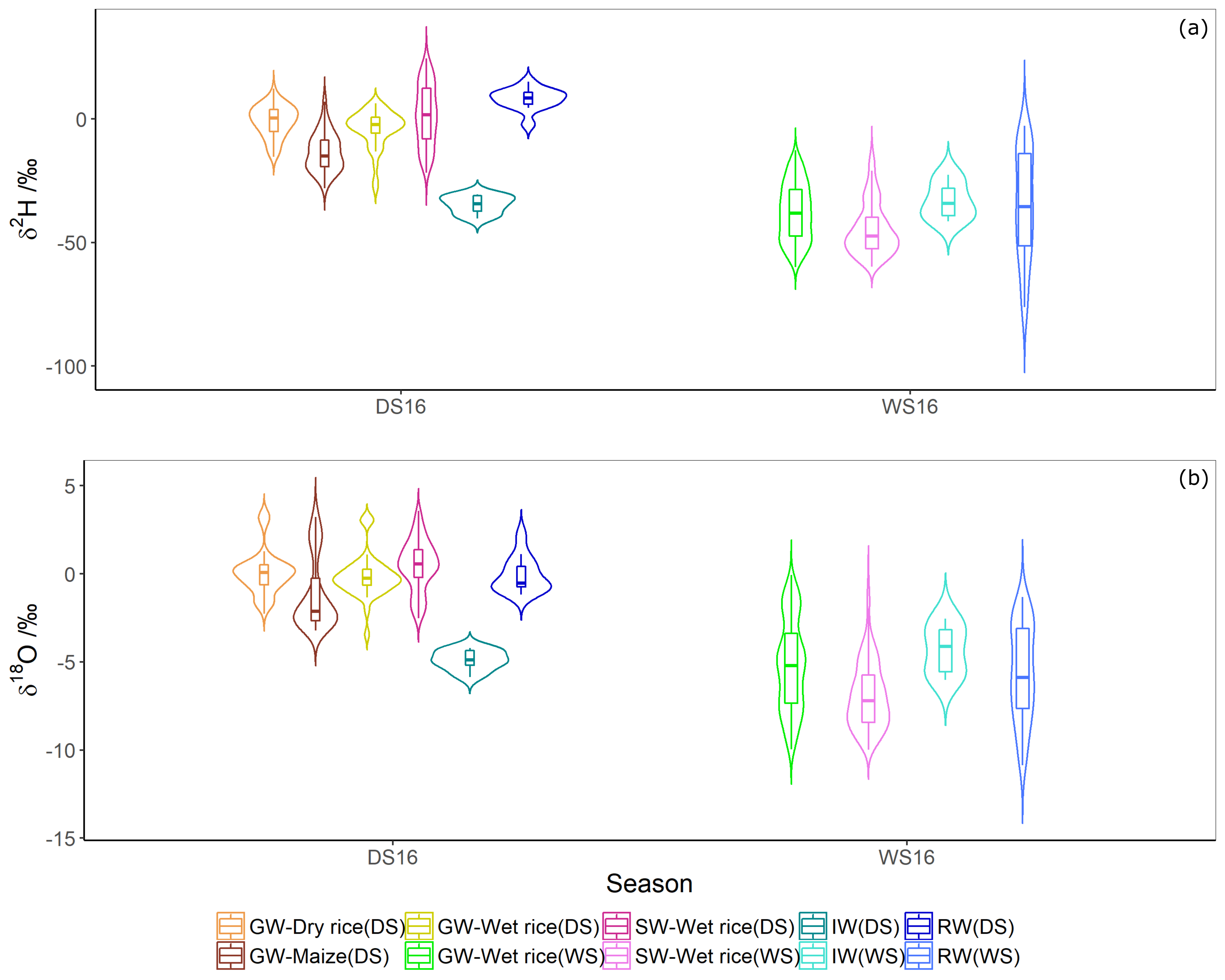
• There are seasonal and crop effects on isotopic compositions in groundwater and surface water.
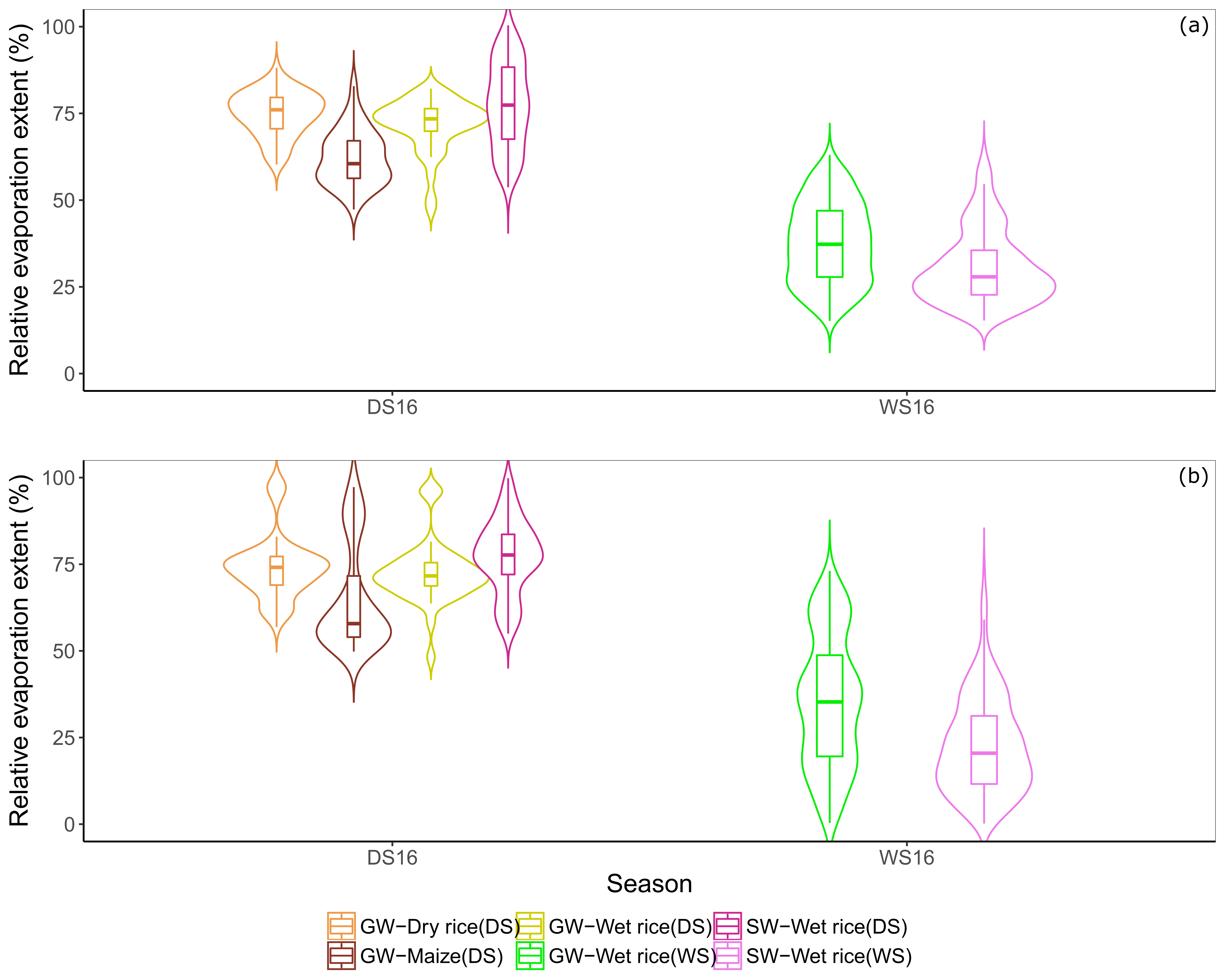
• The isotopic differences in water sources are driven by the evaporation fractionation process.
• Meteorological conditions control evaporation so that a day-night cycle is apparent for stable isotopes of ponding water, while this cannot be found for groundwater.

2. Materials and Methods

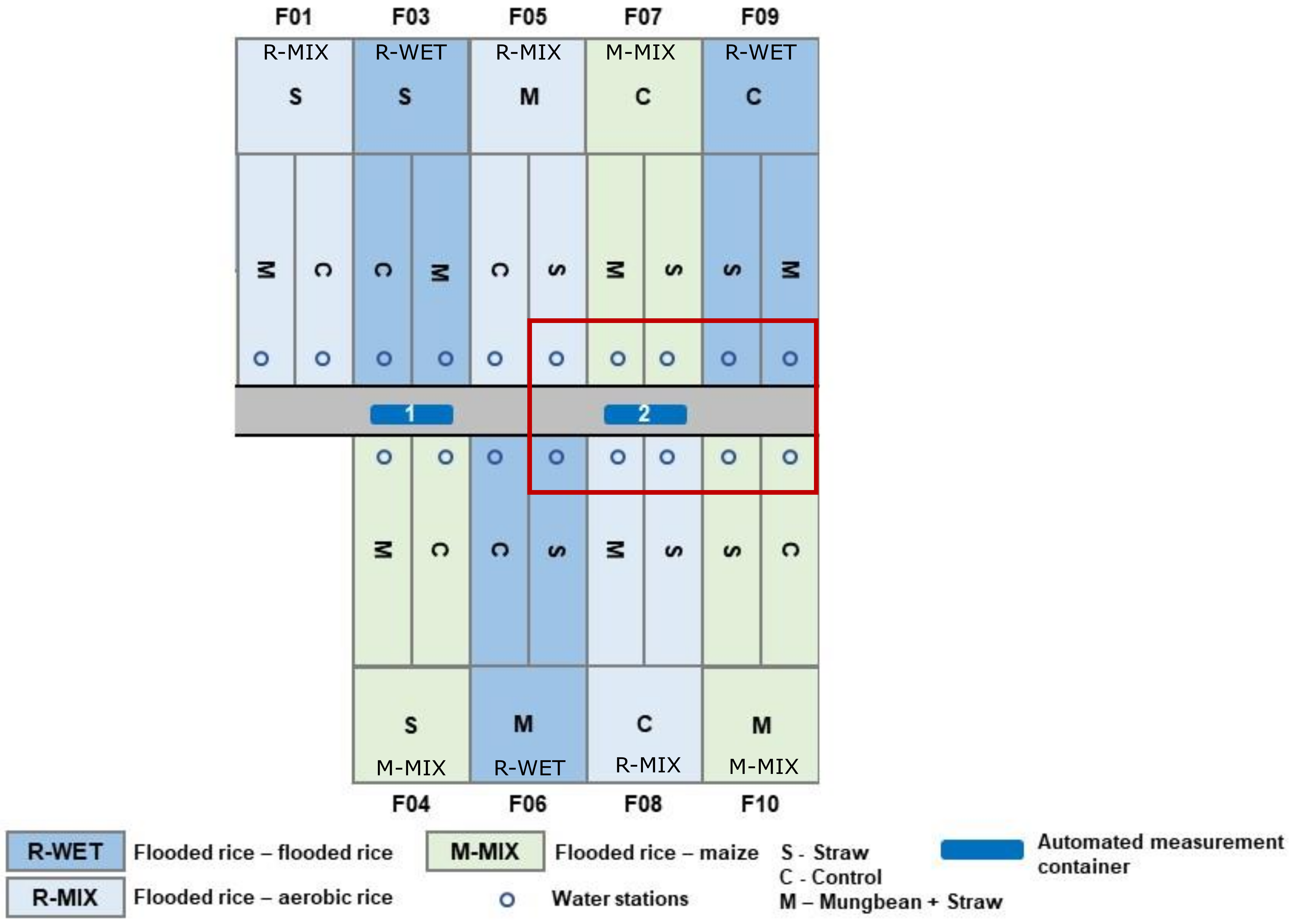
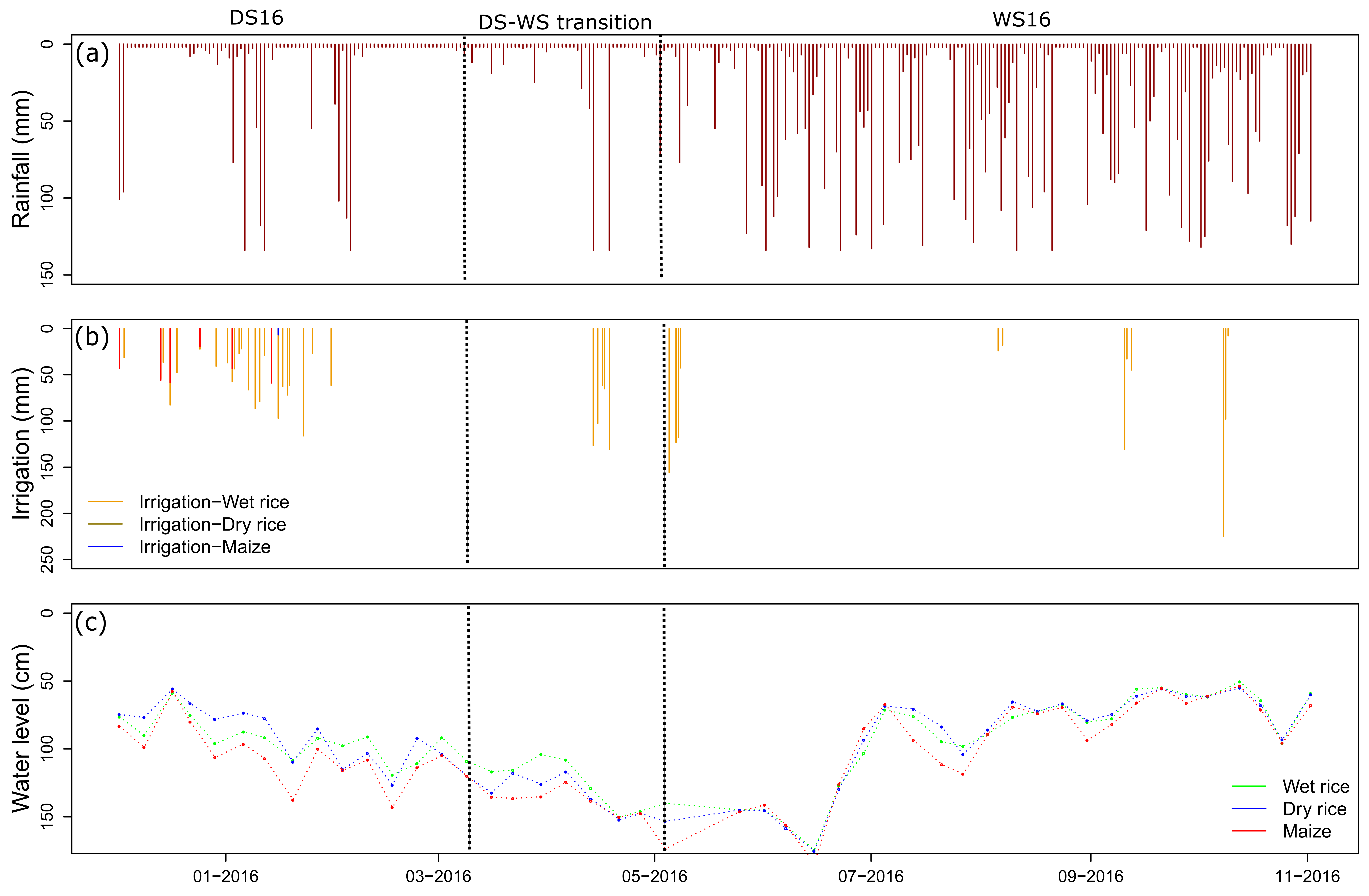
2.1. Field Site and Management

The study was set up on experimental fields at the International Rice Research Institute (IRRI) in Los Baños, Laguna, Philippines (14°11′ N, 121°15′ E, 21 m.a.s.l.) as part of the ICON project (Introducing Non-Flooded Crops in Rice-Dominated Landscapes: Impact on Carbon, Nitrogen and Water Cycles), which focuses on the ecological impact of future climate changes in rice production in South-East Asia. Field measurements were carried out during the dry and wet season from March to October 2016 using the automatic analytical system outlined by Heinz et al. [41]. High-frequency RH and T measurements were utilized and recorded every 30 min by RH and T probes (HMP45C, Campbell Scientific, Inc., Logan, UT 84321-1784, USA) that were connected to an eddy covariance system by Aleberto et al., [49] next to our experimental site. The mean annual temperature was 28.4 ± 1.5 °C, and the seasonal mean of RH was 74 ± 11% during the dry season, which was lower than 82 ± 9% during the wet season of 2016. Precipitation events were more frequent during the wet season, including heavy events. According to the climate data recorded by the Climate Unit at IRRI (IRRI Climate Unit, 2016), average recorded rainfalls were 300 ± 25 mm during the dry season (December–May) and 1700 ± 50 mm during the wet season (July–December). Wind speed was 1.57 ± 0.5 ms⁻¹ during the dry season and 1.13 ± 0.6 ms⁻¹ during the wet season.

The experimental design (Figure 1) consisted of nine paddies with an average field size of around 540 m². During the wet season, all fields were cultivated with wet rice (cultivar NSIC Rc222), while during the dry season, three fields each were cultivated with wet rice (Field code: R-WET), dry rice (cultivar NSIC Rc192) (Field code: R-MIX), and maize (Pioneer P3482YR) (Field code: M-MIX). The whole study site has been cultivated by wet rice (R-WET) for 50 years until 2011. Starting with wet season 2011, our experimental fields were established and from the dry season 2012 onwards, maize and dry rice were cropped during the dry seasons. Each field was homogeneously cultivated with one crop, subjected to the same water and nutrient management regime, and further subdivided into three plots (170–190 m²). Each plot was treated differently, one with straw incorporation to the soil (S), one with straw plus mung bean as an inter-crop in the dry-to-wet transition period (M), and a control plot (C) without any treatment. A total of 130 kg N ha⁻¹ urea was applied over three fertilization dates (30/50/50 kg N ha⁻¹) per plot. Transplant and harvest dates were 8 January and 20 April for dry and wet rice, 6 January and 2 May for maize during the 2016 dry season, and 21 July and 30 October for wet rice during the 2016 wet season. Initial land preparation consists of four phases (and all fields were irrigated during the process): land soaking and straw incorporation at straw fields, plowing and harrowing, a second straw incorporation, ending with a final leveling for transplanting [50]. Paddy bunds were used to separate the fields hydrologically above ground, and plastic sheets were installed inside the bunds 0.3 m below ground. In wet rice fields, flooded water conditions were maintained throughout the growing period, except for the first and last two weeks. During this time, flooded rice fields were regularly irrigated (approximately every 3–5 days) depending on local weather conditions, while dry rice fields were irrigated to maintain the wet soil conditions, approximately once in a week. Maize fields were only irrigated under dry spells if the soils were too dry. Pumped groundwater from the surrounding area was stored in a small reservoir and used as irrigation water. Irrigation during the wet season mainly depends on precipitation amounts, because irrigation was only applied to maintain flooded conditions when necessary. Fields were less frequently irrigated during the wet season than the dry season (Figure 2b). The total irrigation amounts during the dry season were 2015, 840, and 115 m³ for wet rice, dry rice, and maize fields, respectively, and 1525 m³ for all wet rice fields during the wet season.

During the entire sampling period, groundwater levels were measured weekly with an electric contact gauge from the surface level (0 m). Groundwater depth (Figure 2c) below the surface declined from 0.55 ± 0.05 to 1.30 ± 0.1 m until the end of the dry season, then it decreased to 1.70 ± 0.05 m during the transition period from dry season to wet season. The groundwater level of maize was 0.15 ± 0.1 m lower than the wet and dry rice fields during the dry season. During the wet season, groundwater levels fluctuated around 0.70 ± 0.15 m. The soil type at the study area was classified by He et al. [51] as a hydragric anthrosol. The soil contains mostly clay (vermiculite, smectite, and kaolinite). The soil’s average bulk density in the wet rice fields is 0.92 ± 0.03 g cm⁻³ at 0–0.1 m and is 1.02 ± 0.03 g cm⁻³ at 0.1–0.2 m, and in the maize fields, it is 1.17 ± 0.02 g cm⁻³ at 0–0.1 m and 1.13 ± 0.04 g cm⁻³ at 0.1–0.3 m.

2.2. Automatic Analytical System

As described by Heinz et al. [41], the water sampling stations consisted of water level gauges for surface water (surface ponded water) and groundwater, made of common 4″ and 3″ PVC pipes. The installation lengths below ground were 0.2 m for surface water and 2.0 m for groundwater. Low-cost car wiper pumps (Art. Nr. 103 158, TOPRAN, Bremen, Germany) were used to pump water from these multiple sampling stations to container 2 (Figure 1), with a pumping rate of 40 L h⁻¹. The water flow of the system was controlled with a pump/valve system consisting of an industrial computer, a field Input/Output system, and Python controller software that was developed by the authors. The details of the system are given in [41]. The sampling system has been slightly enhanced by replacing non-return valves with solenoid valves to seal unused sources from sampling, and a reservoir was filled to store sample water for continuous water supply and longer measurements. Samples were measured in high temporal resolution (30 min per source) from 12 sources, including five groundwater and five surface water sources, and two standards (standard high and standard low) used as reference water. The sampling frequency of a single source is, therefore, once per 6 h.

2.3. Isotopic Analysis

To analyze the stable isotope composition, we ran wavelength-scanned cavity ring-down spectroscopy (WS-CRDS) (L2120-i, Picarro, Santa Clara, CA, USA) in situ in container 2 (Figure 1). This system measured δ²H and δ¹⁸O in water vapor. Liquid water needs to be carefully vaporized to avoid uncontrolled isotopic fractionation. One option, usually employed in lab systems, is to inject a small water volume (1–2 μL) into a so-called vaporizer and ensure complete vaporization, therefore avoiding fractionation. This approach was used in our original setup [41]; however, the small capillaries of the injection system were not able to handle occasional sediment pollution in the rough conditions of an on-line system. Munksgaard et al. [44] developed another approach, using a porous tube in a dry gas-flooded chamber. The water flowing through the porous tube diffuses into the chamber and vaporizes into the dry gas, thereby changing its isotopic values by fractionation. When the water stream, air stream, and temperature are controlled, the fractionation is also controlled and can be calculated from measuring standards. In this study, we used a custom-made diffusion sampler built by Munksgaard. The sample water flow is delivered by a peristaltic pump (PLP380, Behr Labortechnik, Düsseldorf, Germany) and delivers 0.005 L min⁻¹ of sample water from the reservoir through the diffusion cell.

Additionally, water samples from all sources were collected manually from the sampling stations on a weekly basis in order to (i) verify measurements from the field analytical system and (ii) fill data gaps in case of system failure during system maintenance. A precipitation collector for sampling rainwater was installed on the roof of container 2, with a funnel width of 0.3 m diameter, covered with a mosquito net to avoid contamination. In order to reduce evaporation, the sample storage bottle (1 L polypropylene) was placed inside the air-conditioned container. Rainwater and irrigation water were collected depending on availability. All water samples were collected following the IAEA (International Atomic Energy Agency) standard procedures [52] in 50 mL plastic bottles (Nalgene) and stored under cooled conditions. Manually collected water samples and standards were analyzed for δ²H and δ¹⁸O via a second WS-CRDS process (L2130-i, Picarro, Santa Clara, CA, USA) at the Institute for Landscape Ecology and Resources Management at the Justus Liebig University Giessen, Germany (analytic precisions for δ¹⁸O and δ²H are 0.07‰ and 0.03‰, respectively).

Isotopic compositions are reported as ratios (R) (²H/H, ¹⁸O/¹⁶O) expressed in delta notation (δ,‰) relative to the Vienna Standard Mean Ocean Water (VSMOW) [7]: δ_sample = (R/R_VSMOW − 1). The global meteoric water line (GMWL) was calculated following Rozanski et al. [53] as δ²H = 8.2 δ¹⁸O + 11.3, which is updated from its original form δ²H = 8 δ¹⁸O + 10 [54]. The local meteoric water line (LMWL) [55] was calculated, as δ²H = 7.52 δ¹⁸O + 5.86, according to the local precipitation data from the period 2000–2015 (Global Network of Isotopes in Precipitation of the IAEA, GNIP-IAEA 2016), following the un-weighted ordinary least squares regression method as described in Crawford et al. [56] (Equations (2) and (7)). Linear correlations in a dual isotope coordinate system (δ¹⁸O, δ²H) were calculated for each data cluster (e.g., rainwater, irrigation water and groundwater, and surface water of each crop).

2.4. Raw Data Correction and Calibration

The spectrometer measures the isotopic composition of the water vapor at 1.7 s intervals. To obtain a stable value of the isotopic vapor, the change rate of the water concentration and both isotopic values were analyzed. Identifying these change rates allows us to distinguish between signals where vapor from the last and current sample are mixed (memory effect) and signals from the actual sample only. For both isotope values, the time series from one sample to the next was defined by a sigmoidal function with a lag time in the beginning, a positive slope phase in the transition period, and a plateau in the end. The time needed to reach the plateau varies depending on the signal difference and the system state. The software detected a plateau when the following conditions for a 180 s subset of the time series were met:

• The sample has already been in the diffusion cell for at least 300 s (and therefore safely beyond the lag time).
• The slope of a linear regression for the δ signals as a function of time is less than 0.002‰ s⁻¹ for ²H and 0.005‰ s⁻¹ for ¹⁸O.
• The coefficient of determination (R²) of the δ signals is less than 0.05 over plateau time.
• The vapor content is above 15,000 ppm.

Condition 1 helped to avoid the lag period being detected as the target plateau. Conditions 2 and 3 detected changes in the signal, and condition 4 tested for the proper functioning of the cell. The average of the first 180 s interval, where these conditions were met, was used as the vapor signal.

Raw data from the analytical system were corrected and normalized by applying the method proposed by van Geldern and Barth [57]. To quantify the fraction process in the porous tube, two different, self-produced tertiary standards were sampled by the system twice per day. Laboratory reverse osmosis (RO) water was used as standard low water (isotopically depleted), and in a dry oven evaporated RO water was used as a standard high water (isotopically enriched) and stored in sealed polyethylene bags (10 L) originally produced for gas sampling. Over the measurement time we consumed and reproduced two batches of low standard with δ²H (δ¹⁸O) values of −44.71 (−6.56), −62.24 (−9.24), and three batches of high standard with δ²H (δ¹⁸O) values of −11.36 (1.16), −3.08 (2.34), −12.50 (0.65), respectively, during the experimental period. The temperature and vapor inflow to the system were kept constant, and the measurements were recorded when there was a constant signal height in the detector to avoid the linearity effect [58]. The standard measurements were smoothed over time to avoid overfitting and filtered for system failures. We performed a linear interpolation between the smoothed isotopic values for the fractionated standard water vapor to account for continuous drifts of the instrument and the porous tube chamber state, and get as a result a continuous function over time of standard isotope vapor value for both standards. The standards were also measured in our lab in Germany with a Picarro L2130 with vaporizer injection. The isotopic values for the liquid water from the lab were used together with the continuous interpolation of the water vapor values to do a linear transformation of the measured vapor values from the source samples back to their values prior to fractionation in the porous tube. Additional data filtration was carried out to minimize the noise, applying the thresholds as the slope of the linear regression as 0–2.5, for the dry season: −40–30‰ and −3.5–4‰ for δ²H and δ¹⁸O, respectively, and for the wet season: −60–−10‰, and −10–0‰ for δ²H and δ¹⁸O, respectively, according to the manual sampling data. These calibrated system data were used to test all the hypotheses, and the variations with time and between crops were used to test the seasonal and crop effect on isotopic composition as stated in hypothesis 1. Overall, we recorded 1082 quality-checked measurements during the sampling period that provided the basis for the following analyses.

2.5. Statistical Analysis

The Shapiro–Wilk test was used to test the data for normal distribution, and then the homogeneity of variances was tested using the Fligner–Killeen test (R 3.4.3). To check the statistically significant differences of the water isotopes (δ²H and δ¹⁸O) between all water sources of different crops during both seasons and treatments, the non-parametric rank-based Kruskal–Wallis test was applied, because the data were not normally distributed. A post hoc analysis was performed to determine difference levels of the independent variables. Dunn’s test [59] of multiple comparisons, following a significant Kruskal-Wallis test with the “bonferroni” correction, was carried out to check the pairwise differences, because the Dunn’s test is appropriate for groups with unequal numbers of observations [60]. We rejected the null hypothesis that two crops are significantly different with p ≤ 0.05. A correction for commonalities in the data was considered.

2.6. Estimation of the Relative Extent of Evaporation

In order to test hypothesis 2, the evaporation effect, i.e., the degree of relative extent of source evaporation, was estimated using the equations suggested by Richard [61], applying a simple two-component mixing model with end member analysis.

$${\mathrm{X}}_{\mathrm{E},\mathsf{\delta }}=\frac{{\mathsf{\delta }}_{\mathrm{GW}/\mathrm{SW}}-{\mathsf{\delta }}_{\mathrm{EMDepleted}}}{{\mathsf{\delta }}_{\mathrm{EMEnriched}}-{\mathsf{\delta }}_{\mathrm{EMDepleted}}}$$

(1)

The fraction of relative extent of source evaporation (X_E) of groundwater (GW) and surface water (SW) were calculated referring to the most depleted (EMDepleted) and most enriched (EMEnriched) end member based on δ¹⁸O or δ²H compositions (Equation (1)). Site-specific comparisons of the X_E of various water sources allowed us to estimate the relative extent of evaporation of a recharge source. To account for seasonal effects, we defined fixed, depleted, and evaporated end members for both seasons to have a relative comparison among the sources. The values depend on the assumptions that we made during the calculations [61]: (i) groundwater and surface water are recharged by most depleted rainwater only, and (ii) the end member values are stable in time and are suitable to describe the system for all the samples under different climatic conditions. Therefore, a common end member for each extreme was selected for both seasons. In that case, the most-enriched signatures were selected to represent 100% relative evaporation, which is the SW isotope values from the dry season (δ²H = 24‰ and δ¹⁸O = 3.6‰), and the most-depleted signature representing 0% evaporation, which is the rainwater from the wet season (δ²H = −75‰ and δ¹⁸O = −10‰). These evaporation percentages are only relative values to find the overall extent of evaporation loss from the fields throughout the year. By applying the equations above, we can calculate the evaporation effect for each field and season.

2.7. Assessing Water Provenance of Surface and Groundwater

Back projection of δ¹⁸O for evaporative enrichment was applied to trace the original water source as a correction method for evaporation as part of hypothesis 2. These values are referred to as evaporative corrected values and indicate the isotopic composition without enrichment by evaporation. Each value was interpolated according to the slope of the regression line of each crop following the equation used by Külls [62] from the original equation [63]:

$${\mathsf{\delta }}^{18}{\mathrm{O}}_{\mathrm{corrected}}=\frac{{\mathsf{\delta }}^2{\mathrm{H}}_{\mathrm{measured}}-{\mathrm{e} \mathrm{X} \mathsf{\delta }}^{18}{\mathrm{O}}_{\mathrm{measured}}-\mathrm{d}}{8-\mathrm{e}}$$

(2)

where the e represents the slope of the determined regression line and d is the d-excess of local precipitation. Once the δ¹⁸O had been corrected, the corresponding δ²H values were obtained referring to the LMWL.

During the dry season, rainwater and irrigation water were clear end members to the system; therefore, the evaporation-corrected groundwater isotopic values were used to calculate the fraction of rainwater and irrigation water in groundwater, using the above modified simple-mixing model calculation. The fraction (X) of rainwater (RW) in the groundwater can be written as:

$${\mathrm{X}}_{\mathrm{RW},\mathsf{\delta }}=\frac{\mathsf{\delta }\mathrm{GW}-\mathsf{\delta }\mathrm{IW}}{\mathsf{\delta }\mathrm{RW}-\mathsf{\delta }\mathrm{IW}}$$

(3)

where the δ values represent δ¹⁸O or δ²H values of the evaporative corrected groundwater (GW), measured irrigation water (IW), and rainwater.

2.8. Daily Variation of Isotopic Values

To address hypothesis 3, (the existence of day-night fluctuations in surface water and groundwater isotope composition) days were selected so that at least one observation is available during both daytime (7 a.m. to 7 p.m.) and nighttime (7 p.m. to 7 a.m.). The differences between the daily and nightly mean isotope compositions (δ¹⁸O_day, δ¹⁸O_night) are investigated for each day and for both δ²H and δ¹⁸O. A positive value of the difference indicates higher concentrations of heavy isotopes during the day.

In order to infer whether a day-night pattern exists in the isotopic composition of δ²H and δ¹⁸O, the bootstrapping method was used. In bootstrapping, the aim is to construct an empirical estimate of a sampling distribution of a predefined statistic using Monte Carlo sampling. As we want to know whether there is a clear difference in the magnitude of isotope composition during the day and during the night, we introduce the statistic ${\mathsf{\mu }}_{\mathrm{d}}$, defined as the average value of the differences between daily and nightly isotope composition. A large number of sets is generated, so that each new set is created by randomly selecting n values from the observed set with replacement, with n denoting the number of samples in the observed set. The ${\mathsf{\mu }}_{\mathrm{d}}$ statistic is then calculated for each set. Furthermore, the empirical sampling distribution of the statistic ${\mathsf{\mu }}_{\mathrm{d}}$ is built, which allows us to estimate confidence intervals. By construction, there is a non-zero probability that a value from the observed set is generated more than once in a new generated set.

To investigate, if in this case relative humidity and temperature of the air are also drivers of isotopic composition as in [64] we test if the daily and nightly means and their differences of the atmospheric variables are correlated with the daily and nightly means and their differences of the isotopic composition. The significance of the correlation was tested by calculating p-values using the t-distribution with a significance level of p < 0.05. Correlations with p ≤ 0.01 are defined as highly significant.

3. Results

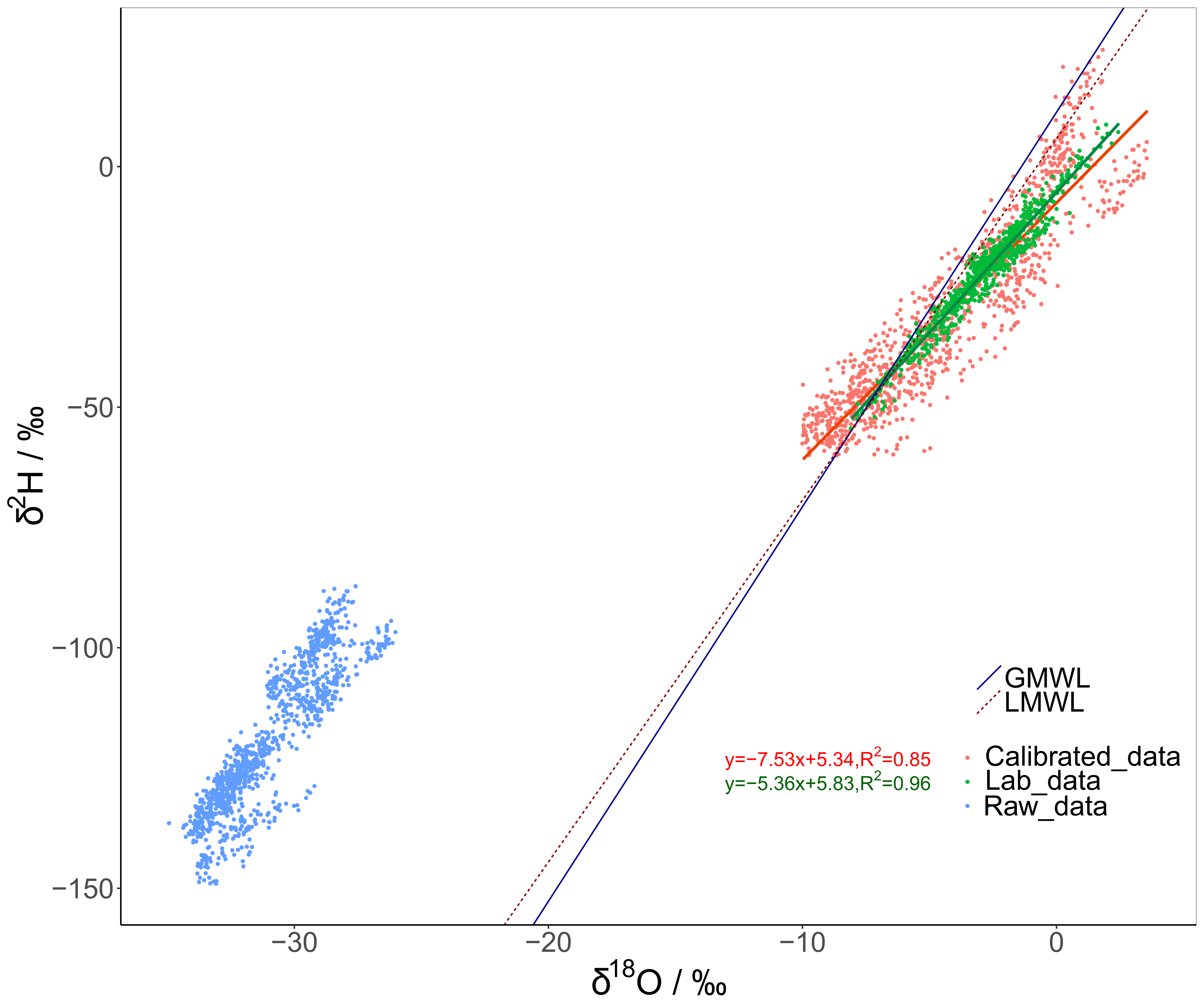
3.1. System Calibrated Data and Lab Data Comparison

Figure 3 demonstrates that the calibrated system data harmonizes well with lab data (manually sampled), with no statistically significant difference. The regression lines were statistically different, with slopes of 5.83 and 5.34, and R² values of 0.96 and 0.85 for lab data and calibrated system data, respectively. There are several reasons for the observed difference between system and lab data: (i) weekly-based manual samples were taken at different times than the system data. The system measured data include not only daytime but also nighttime measurements, while lab data were sampled only during daytime (9–11 a.m.). (ii) System data were based on water vapor measurements mixed with dry gas while lab data were based on liquid water measurements. (iii) Lab data were normalized using laboratory standards while we used self-produced standards in the field-sampling system. Calibrated data in the lower region were plotted on the left side of the LMWL in the figure. This may be due to an instrumental drift because we measured the water vapor instead of liquid water and due to uncertainties in the calibration process. However, this does not affect our goal to compare the different sources and understand the processes on a farming site both spatially and temporally. The width of the uncertainty remains the same throughout the data range. Manually collected lab data are presented in Figure 4. The lab and system data reflect the same pattern based on crop and season although there is a small shift. The mean value of lab data for the dry season and wet season crops are −16.2 ± 9.2 (−2.0 ± 1.5) and −28.3 ± 10.4 (−3.8 ± 1.9) for δ²H (δ¹⁸O), respectively. Therefore, for further analysis, we only use the high-frequency system measured data.

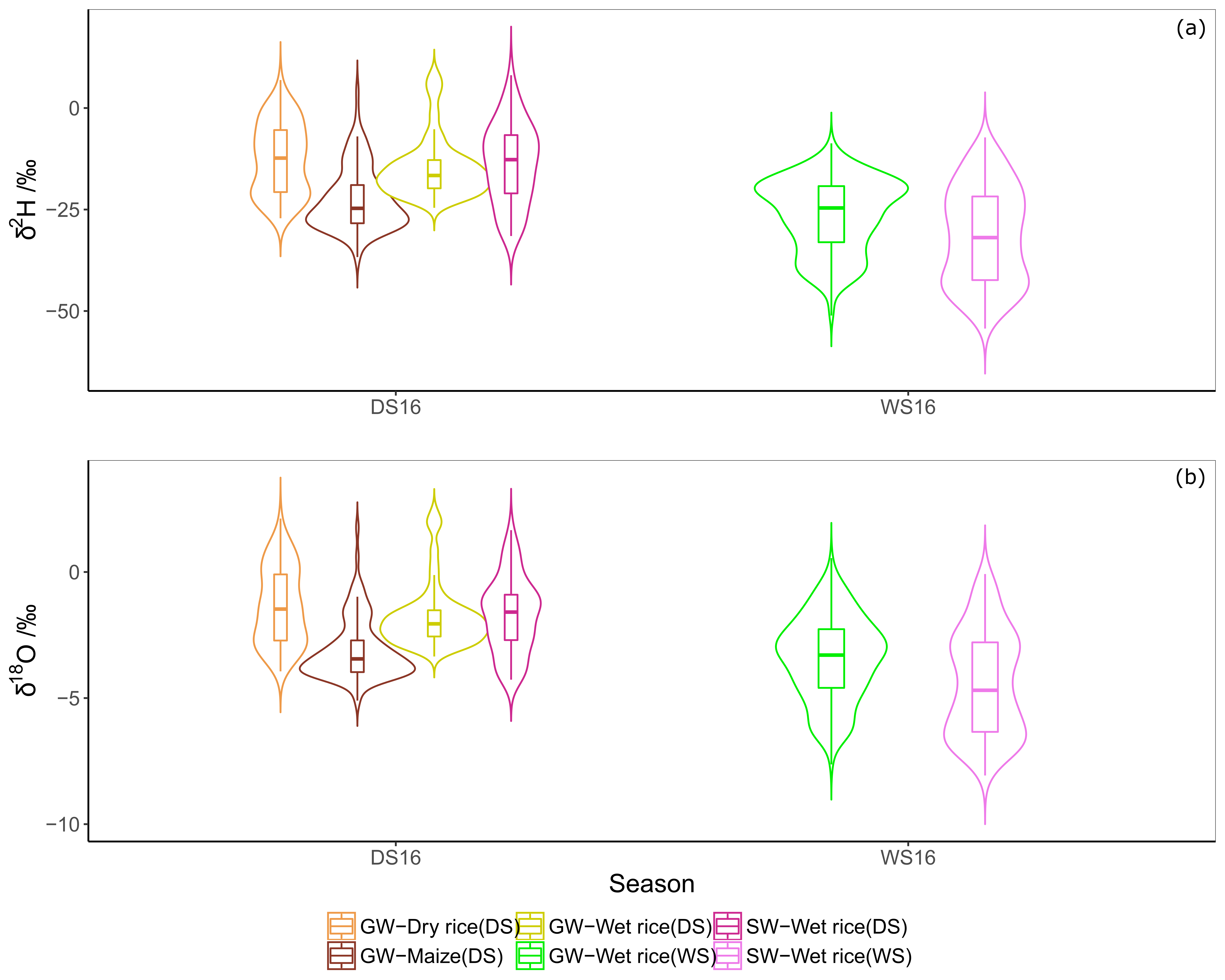
3.2. Isotope Composition of Crops

The differences between treatments of each source within the same crop were not significant (average p ≈ 0.1 for each crop). Therefore, we merged the isotope data of the same crops with similar treatments (S, M, C in Figure 1) for further analysis. To test hypothesis 1, the sources were categorized as groundwater of maize, groundwater of wet and dry rice, surface water of wet rice during the dry season, and groundwater and surface water of wet rice during the wet season.

Figure 5 illustrates the isotope value ranges with respect to δ²H and δ¹⁸O during both seasons. The main water provenances of our experimental fields were rainwater and irrigation water. The isotopic composition of rainwater was different in each season (p < 0.01). During the dry season, the isotopic composition of rainwater and irrigation water diverged (p < 0.01), showing the highest and lowest boundaries of the sample data. The mean rainwater isotopic composition of δ²H and δ¹⁸O were 8.07 ± 4.4 and −0.07 ± 1.0‰, respectively, during the dry season without taking precipitation amount into account. Irrigation water was within a similar range of isotopic composition during both seasons, with no statistical significance (p = 0.9, where δ²H values were −34.6 ± 3.5‰ and −33.2 ± 7.4‰, and δ¹⁸O values were −4.9 ± 0.5‰ and −4.3 ± 1.4‰ during the dry season and wet season, respectively). However, during the wet season, irrigation water has the similar isotopic signature as rainwater (p = 0.9). Compositions of δ²H and δ¹⁸O in rainwater ranged from −76.10 to −2.82‰ and from −10.87 to −1.32‰, respectively, which fluctuated strongly throughout the wet season.

The groundwater and surface water isotopic compositions clearly showed a significant difference between seasons (p < 0.01), where dry season values were higher than the wet season. During the dry season, observed isotopic values were lowest for maize, while the highest were observed for the surface water of wet rice (

Table 1. Mean ± standard deviation (SD) and number of observations of calibrated stable isotopes of groundwater (GW) and surface water (SW) from different crops (maize, wet rice, and dry rice) during the dry season (DS) and wet season (WS).

Season	Water Type	Number of Observations	Calibrated Isotopic Values
			δ2H ± SD [‰]	δ18O ± SD [‰]
DS	GW-Wet rice	40	−3.92 ± 7.6	−0.14 ± 1.2
	GW-Dry rice	67	−0.80 ± 6.3	0.07 ± 1.2
	GW-Maize	88	−13.5 ± 7.8	−1.16 ± 2.0
	SW-Wet rice	101	1.54 ± 12.1	0.48 ± 1.4
WS	GW-Wet rice	517	−37.8 ± 11.6	−5.2 ± 2.6
	SW-Wet rice	269	−44.6 ± 10.6	−6.9 ± 1.9

). The range of isotopic values of groundwater wet rice was a bit lower than that of dry rice. However, the isotopic compositions during the dry season were not significantly different between crops.

All isotope values were plotted in a dual isotopic (δ²H, δ¹⁸O) coordinate system in comparison with the LMWL and GMWL (Figure 6) for visual inspection of hypothesis 1. The isotopic compositions measured at all water sources during both seasons presented a clear seasonal statistical difference in dual isotope base even though there is no statistical difference between the slopes of the regression lines. Wet season data were plotted at a lower intercept (−16.3) along the GMWL, while dry season data were plotted at higher intercept (−3.5) with a slightly higher slope of the regression lines (slopes are 4.10 and 4.07 and R² values are 0.76 and 0.39 for the wet season and the dry season, respectively) (Figure 6a). Rainwater isotopic compositions during both seasons differ strongly, where the dry season had a very low slope (1.8) compared to the wet season (8.0). However, slopes of irrigation water during both seasons were nearly similar (6.2 for the dry season and 5.13 for the wet season). The different water sources of crops are shown in a dual isotope plot (Figure 6b). Higher slopes of regression lines for wet rice surface water during both seasons and the low slopes for maize and dry rice were observed.

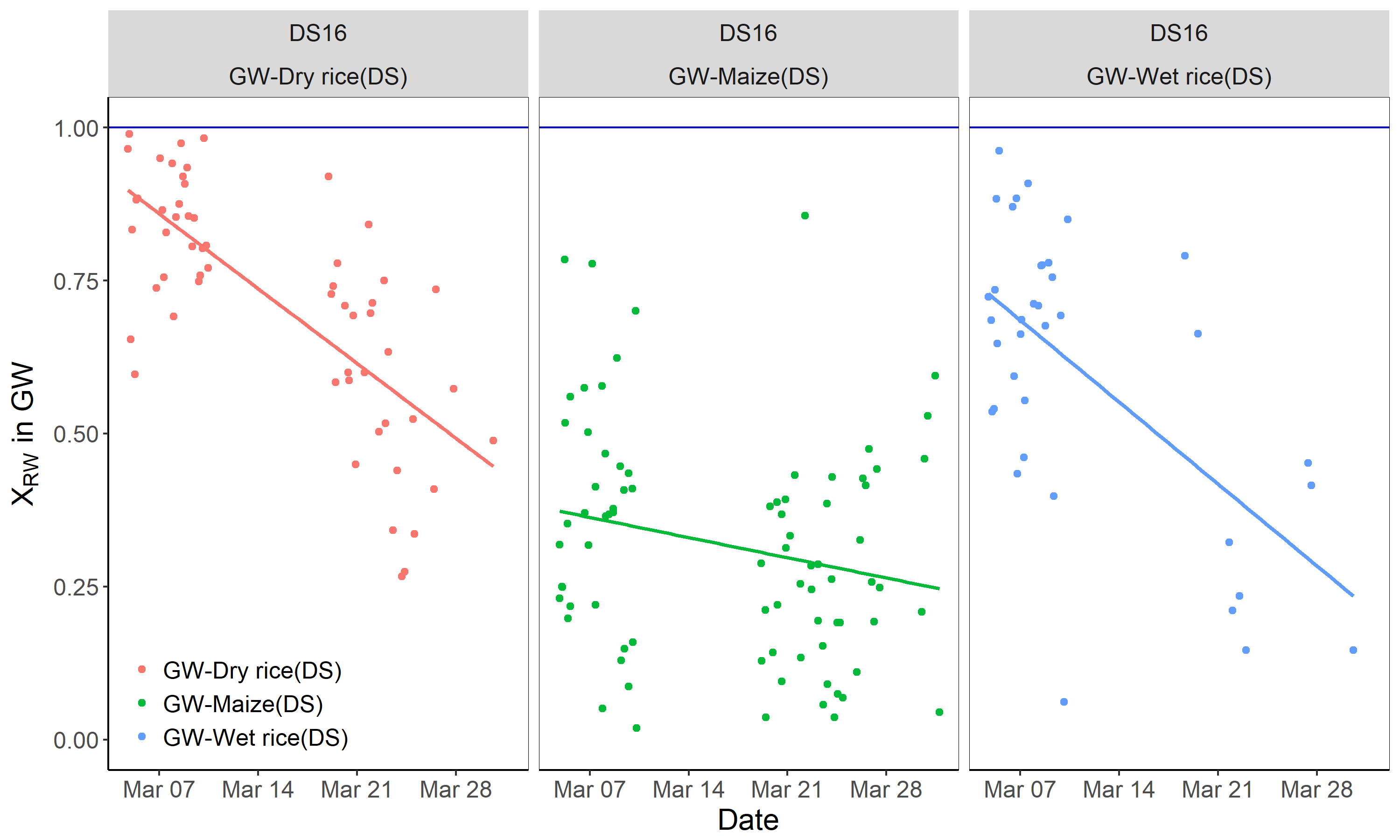
3.3. Estimation of the Relative Extent of Evaporation

The extent of evaporation percentages calculated using Equation (1) are relative to the selected end members and, therefore, the comparison is relative rather than providing absolute values. To understand the effect of the relative evaporation throughout the year, the end members were considered to be representative for the whole year. The relative evaporation was higher during the dry season than during the wet season with regard to both δ²H and δ¹⁸O isotope compositions. During the dry season, the groundwater of maize presented the least evaporative effect (~63%), followed by groundwater of wet (~72%) and dry (~74%) rice fields, while the surface water of wet rice presented the highest evaporated water loss (~77%). Evaporation loss from the groundwater and surface water during the wet season were lower than the dry season, where the relative percentages were ~36% and ~27%, respectively (Figure 7).

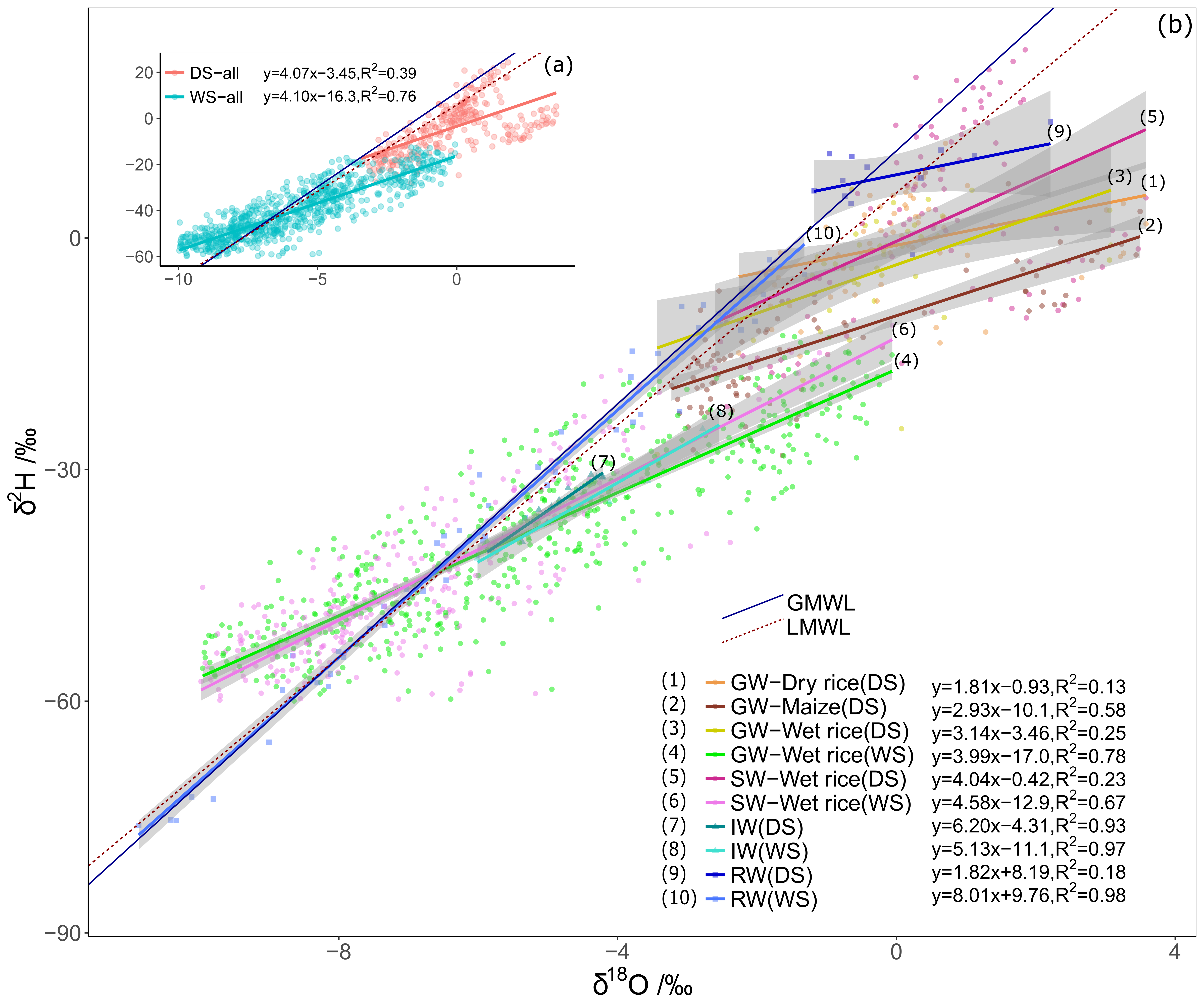
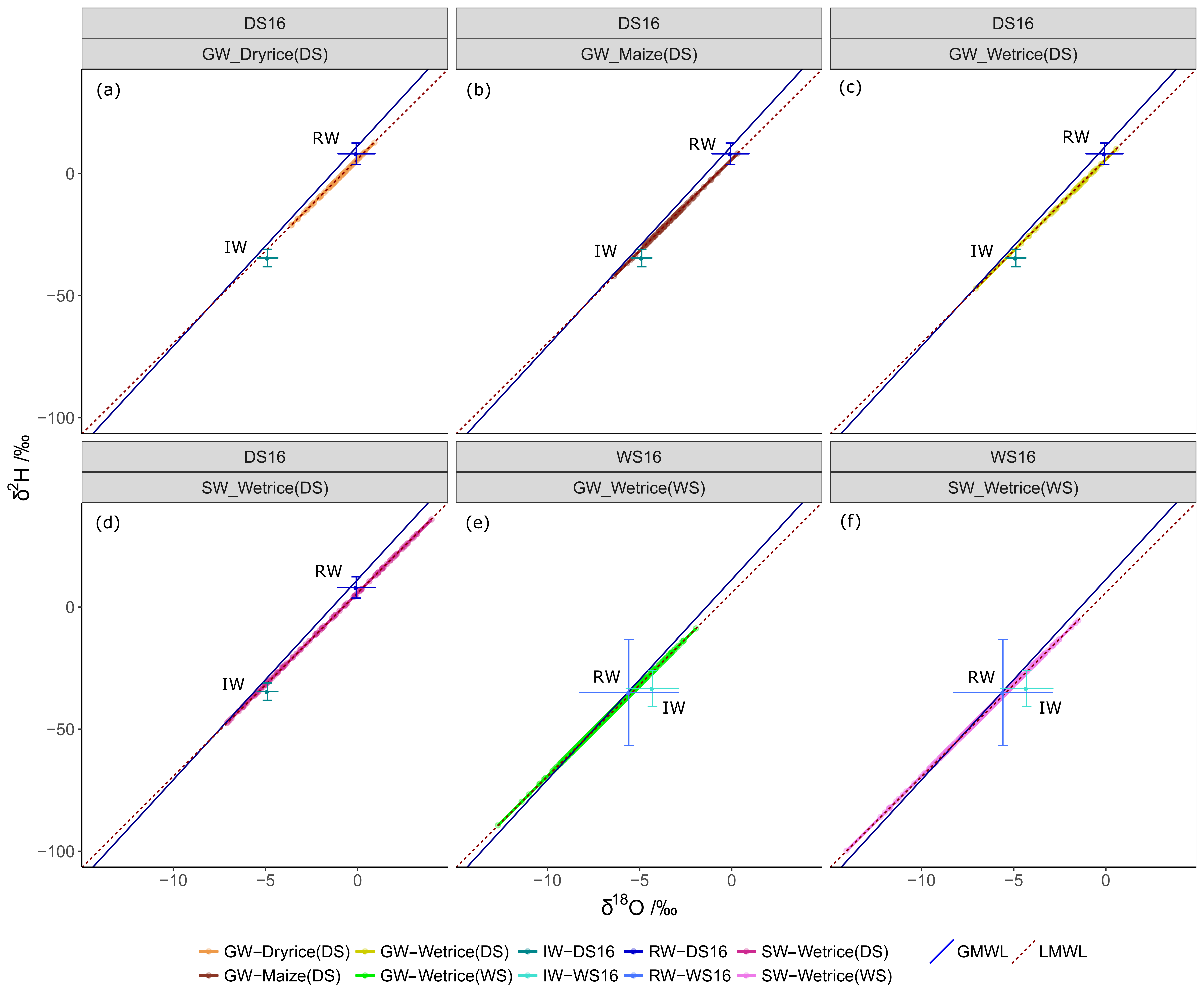
3.4. Assessment of Water Provenance in Surface and Groundwater

To assess the provenance of the sampled surface and groundwater, the measured values from Figure 6 are projected to their respective isotopic signature prior to evaporation using Equation (2). The water sources vary along the LMWL reflecting the seasonal variability of atmospheric moisture provenance and climatic conditions, showing isotopically heavier provenances during the dry season (Figure 8). The projected values have a nearly linear trend with similar ranges that correspond to the season. The average isotope values during the dry season were δ²H = −10.3 ± 12.6‰, and δ¹⁸O = −2.14 ± 1.68‰, and during the wet season, they were δ²H = −42.6 ± 13.6‰ and δ¹⁸O = −6.45 ± 1.81‰. The provenance water (rainwater and irrigation water) represents the proportional water source boundaries (see Section 3.2). Evaporation-corrected isotope values of irrigation water during the dry season were δ²H = −52.4 ± 5.3‰ and δ¹⁸O = −7.77 ± 0.7‰, and during the wet season, they were δ²H = −47.9 ± 4.3‰ and δ¹⁸O = −7.16 ± 0.57‰, where the difference between seasons is not significant. Rainwater isotope values during the dry season were δ²H = 8.96 ± 5.25 and δ¹⁸O = 0.42 ± 0.7‰, while during the wet season they were δ²H = −52.3 ± 44.6‰ and δ¹⁸O = −7.75 ± 5.96‰, with high standard deviations.

The projected isotope values allow a reasonable estimate of the original water provenance for groundwater during the dry season using an end member mixing approach (Equation (3)) to test hypothesis 2. End member mixing is not possible during the wet season, because the end members (rainwater and irrigation water) are not clearly separated (Figure 8e,f). The isotopic signature of the surface water is not bounded by the end members and, therefore, is excluded from the analysis as well. The results of the end member mixing model for each sample are shown in Figure 9 using δ¹⁸O as a tracer. We performed the same analysis with δ²H with similar results. The fraction of rainwater in the groundwater of maize is significantly lower compared to both rice cropping systems (p = 0.05). The fraction of rainwater in the groundwater declines with the duration of the dry season for all crops. While the groundwater of both rice types is composed of 70–80% of rainwater at the start of the high frequency measurements in the middle of the dry season, the rainwater fraction declines with a slope of roughly −0.026 day⁻¹ (p < 0.001) for wet rice and −0.020 day⁻¹ (p < 0.001) for dry rice towards harvest. In the maize fields, rainwater fraction varies between 10–75% (mean 35%) at the beginning and no significant slope (p = 0.08) during the growth.

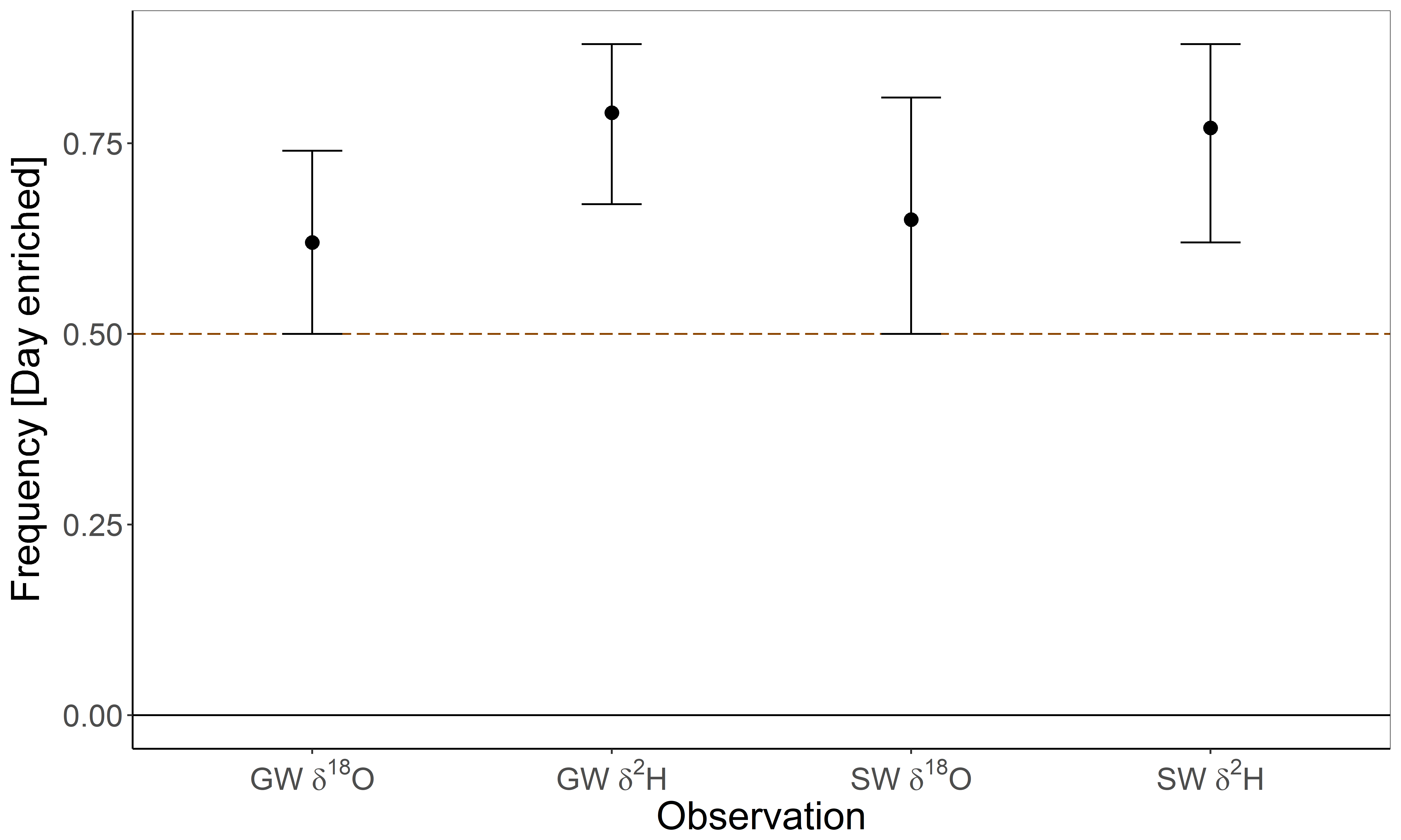
3.5. Daily Variation of Isotopic Values

Analysis carried out for the total sampling period (both wet season and dry season) considering all the crops, showed that daytime isotope composition in groundwater and in surface water is higher than nighttime. There are 45 observation days for groundwater and 26 for surface water, both with sufficient daytime and nighttime measurements for statistical evaluation. Bootstrapping results (Figure 10) show that the expected fraction of time of the δ²H isotope composition is higher during the day for groundwater and surface water: 0.79 (79%) and 0.77 (77%), with associated confidence intervals of [0.67, 0.88] and [0.62, 0.88], respectively. These confidence intervals represent the 5–95% quantiles of the fraction of time for which daily observations are higher than nightly observations. Similar results are observed for δ¹⁸O, with average rates of 0.62 (62%) and 0.65 (65%) and associated confidence intervals of [0.50, 0.74] and [0.50, 0.81] for groundwater and surface water, respectively. These results indicate that the isotope composition is expected to be higher during daytime with 95% confidence. The fraction of time in which the isotope values are higher during the night are 0.21 (21%) and 0.23 (23%) for δ²H in groundwater and in surface water, respectively, with the corresponding confidence intervals of [0.12, 0.33] and [0.12, 0.38]. For δ¹⁸O, these values amount to 0.38 (38%) and 0.35 (35%), with confidence intervals of [0.26, 0.50] and [0.19, 0.50] at the 95% confidence level for groundwater and surface water, respectively. These fractions of time results mean that clearly lower isotopic compositions are observed during the night for both isotopes for both water sources.

Steen et al. [64] show the effect of the atmospheric variables relative humidity (RH) and air temperature (T) on water vapor stable isotopic composition. We tested if the isotope values of surface water and groundwater are also correlated with the atmospheric state and if the difference between daily and nightly mean isotopic compositions can be explained by atmospheric conditions.

The possible correlation between the isotopic composition of daily and nightly values with RH and T, considering combinations such as average values and differences of average values, are presented for groundwater in

Table 2. Correlations between relative humidity (RH) or temperature (T) for different combinations of daily/nightly average values and their differences, and daily/nightly isotopic values (δ²H and δ¹⁸O) in groundwater (GW) (a) and in surface water (SW) (b).

(a)
GW	δ2Hday	δ2Hnight	δ18Oday	δ18Onight	δ2Hday− δ2Hnight	δ18Oday−δ18Onight
RHday	−0.618 **	−0.639 **	−0.675 **	−0.658 **	(0.008)	(−0.083)
RHnight	−0.530 **	−0.547 **	−0.547 **	−0.551 **	(−0.001)	(0.044)
RHday − RHnight	−0.471 **	−0.490 **	−0.567 **	−0.523 **	(0.020)	(−0.256)
Tday	0.395 **	0.408 **	0.491 **	0.471 **	(−0.002)	(0.106)
Tnight	(0.086)	(0.088)	(0.133)	(0.146)	(0.004)	(−0.086)
Tday − Tnight	0.471 **	0.487 **	0.550 **	0.506 **	(−0.008)	(0.263)
(b)
SW	δ2Hday	δ2Hnight	δ18Oday	δ18Onight	δ2Hday − δ2Hnight	δ18Oday − δ18Onight
RHday	−0.679 **	−0.682 **	−0.797 **	−0.785 **	(0.081)	(−0.097)
RHnight	−0.651 **	−0.661 **	−0.781 **	−0.793 **	(0.155)	(0.091)
RHday − RHnight	(−0.331)	(−0.317)	(−0.351)	(−0.292)	(−0.135)	−0.466 *
Tday	(0.345)	(0.354)	0.465 *	0.442 *	(−0.133)	(0.178)
Tnight	(0.123)	(0.138)	(0.261)	(0.271)	(−0.175)	(−0.079)
Tday − Tnight	(0.356)	(0.349)	(0.326)	(0.274)	(0.070)	0.416 *

Correlations with p < 0.01 are marked with **, 0.01 < p < 0.05 with *, and p > 0.05 in parentheses.

a and for surface water in Table 2b. There is a strong negative correlation between the average relative humidity and the average isotope composition in groundwater and in the surface water regarding both day and nighttime, especially for δ¹⁸O. Daily average temperature is significantly positive correlated between daily average isotopic values in groundwater. In the surface water, this correlation is only observed for δ¹⁸O_day. On one hand, the average daily and nightly isotopic values in groundwater revealed a high correlation with average daily and nightly differences of RH (R = −0.51) and T (R = 0.50); on the other hand, it is significant only with relative humidity in surface water. The isotopic differences of the daily and nightly mean values in the groundwater cannot be explained by these parameters. However, the δ¹⁸O day-night differences in surface water are correlated with RH and T day-night differences.

Sub-daily isotopic fluctuation in surface water was expected as by hypothesis 3 for surface water; however, surprisingly, that is also true for groundwater, which challenged hypothesis 3 for groundwater.

4. Discussion

4.1. Isotope Composition of Water Sources

Hypothesis 1 is confirmed by the results, which show that the isotopic compositions have responded to the seasonal and crop changes. The isotopic compositions were more enriched (higher values) during the dry season than the wet season (Figure 5), making an indicative signal of evaporation during warmer and drier periods [65]. A greater seasonality in evaporative fractionation [66] can also be perceived in the isotopic composition of rainwater (Figure 6), where most of the rainwater measurements during the wet season fall on or near the LMWL (but during the dry season, significant deviations occurred by more isotopically enriched samples. Climatic conditions during the dry season were slightly warmer and less humid with fewer precipitation events, as represented by the low slope of the regression line [67] compared to the wet season. The relative humidity variation during drier periods creates a stronger evaporative effect, thereby inducing more water loss in rice paddies. With decreasing relative humidity, an increase in the enrichment of δ¹⁸O in the plant leaf was reported in grass species [68] and trees [69] which may also affect the water sources. The relative humidity and temperature alter the slopes of evaporation regression lines, and the slope under the relative humidity values between 25–75% would be ~5 for open water bodies [65], where we observed ~4 for surface water during both seasons under the relative humidity values between 65–90%. The amount evaporated depends on the time of exposure to the atmosphere and the meteorological conditions [70]. Surface water during the dry season undergoes more fractionation than during the wet season, which was supported by more-enriched values during the dry season. In contrast, lower slopes (~2) have been encountered for soil moisture [65], for which we observed similar slopes (~2) for maize and dry rice groundwater. This can be due to the dryer soil conditions, which causes such water to show greater relative enrichment of ¹⁸O over ²H when compared to meteoric waters [71].

The crop-wise groundwater isotopic composition differences were prominent during the dry season. The trend of isotopic enrichment was observed subsequently from groundwater of maize and groundwater of wet and dry rice to the surface water of wet rice, which were derived from the main water input, i.e., irrigation water (Figure 5). The groundwater was predominantly recharged by irrigation water during this time due to less frequent, short rain events, which are evaporated quickly. The groundwater were more enriched than the irrigation water, signifying the subsequent enrichment of irrigation water throughout the infiltration process. A similar enrichment process in groundwater via irrigation water was observed in the lower Okanagan valley in Canada [45]. The possible facts which course the isotopic enrichment process via recharge could be (i) partial evaporation of irrigation water by vapor diffusion during its residence in the unsaturated topsoil [72], (ii) fractionation via root water uptake [73,74], and (iii) fractionation of water during passage through compacted clayey sediments [75,76,77]. During the wet season, rainwater was the main water supply to the fields due to the frequent long rain events. Because all the fields were maintained flooded, the main direct recharge source of groundwater was the more relatively evaporated ponded surface water. Due to the numerous mixing incidences between surface water with rainwater during this time, the ponded surface water was again being depleted compared to the groundwater. This frequently-added rainwater inundates the rice fields, replenishes the groundwater and surface water, replaces old groundwater, and allows for a better interaction of surface water and groundwater on wet rice fields.

Overall, we could identify temporal statistical differences of isotopic compositions between not only dry and wet seasons, but also between different crops, particularly during the dry season, thus leading to the acceptance of hypothesis 1.

4.2. Relative Evaporation Extent

Small-scale and local isotope composition variations in water are very important for understanding groundwater provenance and identifying recharge mechanisms dependent on the seasonal and temporal changes. With regard to the compositions of isotopically enriched and depleted end members, the simple two-point mixing model enables one to estimate the relative extent of evaporation of a recharge source, which helps for a crop-specific evaporation comparison. Comparatively high relative evaporation losses (>50%) were detected during the dry season due to the evaporated recharge source; during the wet season, this was controlled by isotopically depleted rainwater and the difference in climatic conditions (Figure 7). During the dry season, the evaporation extent differences were governed by meteorological factors [78], such as highly enriched short precipitation events, high wind speed, higher temperature, and lower relative humidity [79]. Most depleted isotopic values and the lowest relative evaporative extent were observed in maize, corresponding to the fact that vegetation type is one of the responsible factors for the intensity of evaporation [80]. Unlike rice plants, maize plants are bigger and have longer and wider leaves with a high leaf area index [81], which adds additional shade and cooling soil conditions. These conditions reduce the evaporation on the ground, which also influences the groundwater conditions. The groundwater isotopic composition of maize was closer to that of the irrigation water than the groundwater of dry or wet rice. This could have happened for two reasons: (i) maize has a deep root system (>0.8 m) [22] by contrast with the shallower and denser root system of rice [18], which can access the deep groundwater that is connected to the surrounding area; or/and (ii) the irrigation water mixes directly with the maize groundwater via cracks [82]. In maize fields, a noticeable feature of the ground was fracturing/cracking of the clayey soil. We conducted an additional crack experiment to check the differences of cracks in the fields, and results show that the cracks in maize fields were deeper (0.2 m) and narrower (0.02 m) than in rice fields. The least irrigated crop was maize, which made room to develop cracks, hence the irrigation water could directly flow along the cracks and mix with groundwater with less hydraulic retention time. Relative evaporation extent for maize fields (63%) was consistent with the other studies, where 54% were observed in southern California [81] and 78% in China [25]. Wet rice fields have a similar evapotranspiration (72%) to dry rice fields (74%) during the dry season, which decreases to 36% during the wet season. Simpson et al. [5] observed 40% water loss caused only from evaporation [5], from wet rice fields in a semi-arid region of south-eastern Australia, which is comparable to our findings. The most-enriched isotopic values and the highest relative evaporative extent (77%) were observed in the surface water of wet rice during the dry season, where the evaporation was considered a key factor affecting the isotopic composition of surface water [83]. Because newly evaporated water vapor is no longer in equilibrium with the open water body of origin [84], the water phase becomes enriched with heavy isotopes when relative humidity is less than 100% [78]. Accepting hypothesis 2, where we confirmed an evaporation fractionation effect, leads us to further correct data to explore the isotopic spreading in a non-evaporated space. This we applied to identify the water input fractions of rainwater and irrigation water in the groundwater during the dry season.

4.3. Origin of Water Sources

We back projected each data point to find out the origin of the water sources, following the method of Geyh et al. [63] and Külls et al. [62]. The variances of the evaporation-corrected original water sources are narrower in the dry season than in the wet season (Figure 8). The clear separation of the isotopic signal of the end members irrigation water and rainwater allowed for tracking their crop-specific contribution to groundwater over time. Figure 9 shows a large contribution of rainwater to the groundwater in the middle of the season, which declines towards the harvest date under dry and wet rice. Groundwater below maize reacts differently: on average, the rainwater contribution is smaller, the trend over time is weak, and the variation is much smaller. If we recall, that the maize fields create deeper cracks (own observation, [85]) with its deeper root system [22] in comparison with rice, these results show a direct connection between irrigation, the few rainfall events, and the groundwater. The puddle layer, created over decades of wet rice cropping on our experimental fields, is broken due to these cracks. Seepage is rapidly transported via cracks through the broken puddle layer to lower soil profiles. Similar results have been found in nearby installed lysimeters by He et al. [85], where maize showed a direct nutrient breakthrough behavior, compared to rice.

4.4. Sub-Daily Fluctuation of Surface and Groundwater

The high frequency in situ measurements clearly differentiated sub-daily fluctuations concerning isotopic compositions of water sources at the irrigation field. Bootstrapping statistical analysis confirms with 95% confidence that the isotope compositions are higher during the daytime, and the sub-daily isotopic compositions were more-enriched than nightly values in groundwater and in surface water throughout the sampling period (Figure 10). The frequency of daytime enrichment is higher for δ²H, which needs less energy than δ¹⁸O for fractionation.

Sub-daily isotopic fluctuations were not yet analyzed before, neither for surface water nor for groundwater. The sub-daily isotopic differences are likely caused by the fractionation of evaporation and can be predicted using the Craig and Gordon model [86]. The model describes the joint effect of equilibrium and kinetic isotopic fractionation during the phase transition from liquid water to vapor. The isotopic enrichment of the water during the daytime is possibly controlled by relative humidity and temperature. The daily and seasonal isotopic fluctuations correspond to diurnal cycles of the atmospheric conditions for open water bodies [87], especially of relative humidity [64,88]. Following our results, the sub-daily patterns of relative humidity and, to a lesser degree, temperature has a strong influence on the sub-daily fluctuation of the isotopic composition in groundwater and surface water (Table 2).

The isotopic day-night difference in groundwater was independent from the six tested atmospheric variables, as shown by the lack of significant correlations (Table 2a). The day-night differences for δ¹⁸O in surface water are correlated with the day-night differences of temperature and relative humidity (Table 2b). Compared to the required energy to be fractionated [89], this may not be sufficient in groundwater as it is in surface water. Maxwell and Condon [90] found that water table depth and lateral groundwater flow influence both latent heat flux and its partitioning into evaporation and transpiration, which may result in isotopic changes in the groundwater and may substantially increase the evaporation fraction of total evapotranspiration. This suggests that groundwater may provide a missing link for evapotranspiration flux partitioning on a sub-daily basis under steady and non-steady conditions. If we follow Maxwell and Condon’s [90] reasoning and with regard to the shallow groundwater table, an enhanced evaporation from the groundwater during daytime is possible, which may lead to an enrichment of the heavy isotopes in the groundwater. At night, lateral flow from regions with deeper groundwater tables could revert the enrichment of the day. However, we are not able to test this explanation with the existing experimental setup.

We accept hypothesis 3 for surface water, but reject for groundwater, because in addition to surface water responses, we observed and tested the groundwater responses to day-night differences. The high-frequency, in situ system, was capable of producing time series of δ¹⁸O and δ²H at sub-hourly temporal resolution from multiple sources for both seasons in 2016 and allowed us to identify the characteristics of hydrological processes in different crops.

5. Conclusions

Measuring the stable isotopes of water using a multi-source and high-frequency system increases the capability of researchers to identify detailed hydrological processes. There is a higher relative evaporation extent and, therefore, greater enrichment process during the dry season than the wet season, revealing great seasonal variability driven by the evaporation fractionation process. The effect of crops on the evaporation process is factual and distinguishable, affecting the enrichment of groundwater. Groundwater in maize is less evaporative affected than in rice due to the direct water flow via cracks or/and deep roots, while the groundwater in rice fields is not affected by these fast water-exchange processes. Due to the management setup and the similarity of irrigation water and rainwater during the wet season, we cannot test if this cropping effect persists into the next cropping season.

We identified isotope enrichment in groundwater and surface water during the daytime, when the relative humidity is low and the temperature is high. However, the day-night isotopic differences in groundwater were driven by neither relative humidity nor temperature, while these meteorological parameters affected the differences of stable isotopes in surface water. The new finding of sub-daily changes of isotopic composition in water sources demonstrates the possibilities provided by high-frequency sampling. It also shows that paying more attention to the sampling time of the day might be relevant to bring together observations with process understanding or theoretical concepts. Advancing the current research to quantify the sub-daily changes for different crops under different climatic conditions for a longer duration, would likely reveal more processes that might take place in irrigation agriculture, particular in specific systems such as rice paddies.

References

1. Maclean, J.L.; Dawe, D.C.; Hettel, G.P. Rice Almanac: Source Book for the Most Important Economic Activity on Earth, 3rd ed.; International Rice Research Institute, Ed.; CABI Publishing: Oxon, UK, 2002; ISBN 978-0-85199-636-3. [Google Scholar]
2. Bouman, B.A.M.; Tuong, T.P. Field water management to save water and increase its productivity in irrigated lowland rice. Agric. Water Manag. 2001, 49, 11–30. [Google Scholar] [CrossRef]
3. Mekonnen, M.M.; Hoekstra, A.Y. The green, blue and grey water footprint of crops and derived crop products. Hydrol. Earth Syst. Sci. 2011, 15, 1577–1600. [Google Scholar] [CrossRef] [Green Version]
4. Zwart, S.J.; Bastiaanssen, W.G.M. Review of measured crop water productivity values for irrigated wheat, rice, cotton and maize. Agric. Water Manag. 2004, 69, 115–133. [Google Scholar] [CrossRef]
5. Simpson, H.J.; Herczeg, A.L.; Meyer, W.S. Stable isotope ratios in irrigation water can estimate rice crop evaporation. Geophys. Res. Lett. 1992, 19, 377–380. [Google Scholar] [CrossRef]
6. Wu, H.; Li, J.; Song, F.; Zhang, Y.; Zhang, H.; Zhang, C.; He, B. Spatial and temporal patterns of stable water isotopes along the Yangtze River during two drought years. Hydrol. Process. 2018, 32, 4–16. [Google Scholar] [CrossRef]
7. Craig, H.; Gordon, L.I. Stable isotopes in oceanographic studies and paleotemperatures. In Spoleto; Tongiorgi, T., Ed.; Laboratory of Geology and Nuclear Science: Spoleto, Italy, 1965; pp. 9–130. [Google Scholar]
8. Klaus, J.; Zehe, E.; Elsner, M.; Külls, C.; McDonnell, J.J. Macropore flow of old water revisited: Experimental insights from a tile-drained hillslope. Hydrol. Earth Syst. Sci. 2013, 17, 103–118. [Google Scholar] [CrossRef] [Green Version]
9. Volkmann, T.H.M.; Weiler, M. Continual in situ monitoring of pore water stable isotopes in the subsurface. Hydrol. Earth Syst. Sci. 2014, 18, 1819–1833. [Google Scholar] [CrossRef] [Green Version]
10. McDonnell, J.J.; Beven, K. Debates—The future of hydrological sciences: A (common) path forward? A call to action aimed at understanding velocities, celerities and residence time distributions of the headwater hydrograph. Water Resour. Res. 2014, 50, 5342–5350. [Google Scholar] [CrossRef]
11. Narancic, B.; Wolfe, B.B.; Pienitz, R.; Meyer, H.; Lamhonwah, D. Landscape-gradient assessment of thermokarst lake hydrology using water isotope tracers. J. Hydrol. 2017, 545, 327–338. [Google Scholar] [CrossRef] [Green Version]
12. Sprenger, M.; Tetzlaff, D.; Soulsby, C. Stable isotopes reveal evaporation dynamics at the soil-plant-atmosphere interface of the critical zone. Hydrol. Earth Syst. Sci. Discuss. 2017, 1–37. [Google Scholar] [CrossRef]
13. Darling, W.G.; Bowes, M.J. A long-term study of stable isotopes as tracers of processes governing water flow and quality in a lowland river basin: The upper Thames, UK. Hydrol. Process. 2016, 30, 2178–2195. [Google Scholar] [CrossRef] [Green Version]
14. McGuire, K.J.; McDonnell, J.J. Tracer advances in catchment hydrology. Hydrol. Process. 2015, 29, 5135–5138. [Google Scholar] [CrossRef]
15. Chung, I.-M.; Kim, J.-K.; Prabakaran, M.; Yang, J.-H.; Kim, S.-H. Authenticity of rice (Oryza sativa L.) geographical origin based on analysis of C, N, O and S stable isotope ratios: A preliminary case report in Korea, China and Philippine. J. Sci. Food Agric. 2016, 96, 2433–2439. [Google Scholar] [CrossRef] [PubMed]
16. Kaushal, R.; Ghosh, P. Stable Oxygen and Carbon Isotopic Composition of Rice (Oryza sativa L.) Grains as Recorder of Relative Humidity. J. Geophys. Res. Biogeosci. 2018. [Google Scholar] [CrossRef]
17. Akamatsu, F.; Suzuki, Y.; Nakashita, R.; Korenaga, T. Responses of carbon and oxygen stable isotopes in rice grain (Oryza sativa L.) to an increase in air temperature during grain filling in the Japanese archipelago. Ecol. Res. 2014, 29, 45–53. [Google Scholar] [CrossRef]
18. Mahindawansha, A.; Orlowski, N.; Kraft, P.; Rothfuss, Y.; Racela, H.; Breuer, L. Quantification of plant water uptake by water stable isotopes in rice paddy systems. Plant Soil 2018. [Google Scholar] [CrossRef]
19. Wei, Z.; Lee, X.; Wen, X.; Xiao, W. Evapotranspiration partitioning for three agro-ecosystems with contrasting moisture conditions: A comparison of an isotope method and a two-source model calculation. Agric. For. Meteorol. 2018, 252, 296–310. [Google Scholar] [CrossRef]
20. Brunel, J.P.; Simpson, H.J.; Herczeg, A.L.; Whitehead, R.; Walker, G.R. Stable isotope composition of water vapor as an indicator of transpiration fluxes from rice crops. Water Resour. Res. 1992, 28, 1407–1416. [Google Scholar] [CrossRef]
21. Wu, Y.; Du, T.; Li, F.; Li, S.; Ding, R.; Tong, L. Quantification of maize water uptake from different layers and root zones under alternate furrow irrigation using stable oxygen isotope. Agric. Water Manag. 2016, 168, 35–44. [Google Scholar] [CrossRef]
22. Ma, Y.; Song, X. Using stable isotopes to determine seasonal variations in water uptake of summer maize under different fertilization treatments. Sci. Total Environ. 2016, 550, 471–483. [Google Scholar] [CrossRef] [PubMed] [Green Version]
23. Zhao, X.; Li, F.; Ai, Z.; Li, J.; Gu, C. Stable isotope evidences for identifying crop water uptake in a typical winter wheat-summer maize rotation field in the North China Plain. Sci. Total Environ. 2018, 618, 121–131. [Google Scholar] [CrossRef] [PubMed]
24. McCool, W.C.; Coltrain, J.B. A Potential Oxygen Isotope Signature of Maize Beer Consumption: An Experimental Pilot Study. Ethnoarchaeology 2018, 10, 56–67. [Google Scholar] [CrossRef]
25. Wu, Y.; Du, T.; Ding, R.; Tong, L.; Li, S.; Wang, L. Multiple Methods to Partition Evapotranspiration in a Maize Field. J. Hydrometeorol. 2017, 18, 139–149. [Google Scholar] [CrossRef] [Green Version]
26. Li, Y.H.; Cui, Y.L. Real-time forecasting of irrigation water requirements of paddy fields. Agric. Water Manag. 1996, 31, 185–193. [Google Scholar] [CrossRef]
27. Trout, T.J.; DeJonge, K.C. Crop Water Use and Crop Coefficients of Maize in the Great Plains. J. Irrig. Drain. Eng. 2018, 144, 04018009. [Google Scholar] [CrossRef]
28. Bouman, B.A.M. Water Management in Irrigated Rice: Coping with Water Scarcity; International Rice Research Institute: Los Baños, Philippines, 2007; ISBN 978-971-22-0219-3.
29. Tabbal, D.F.; Bouman, B.A.M.; Bhuiyan, S.I.; Sibayan, E.B.; Sattar, M.A. On-farm strategies for reducing water input in irrigated rice; case studies in the Philippines. Agric. Water Manag. 2002, 56, 93–112. [Google Scholar] [CrossRef]
30. Tuong, T.P.; Bhuiyan, S.I. Increasing water-use efficiency in rice production: Farm-level perspectives. Agric. Water Manag. 1999, 40, 117–122. [Google Scholar] [CrossRef]
31. Lage, M.; Bamouh, A.; Karrou, M.; El Mourid, M. Estimation of rice evapotranspiration using a microlysimeter technique and comparison with FAO Penman-Monteith and Pan evaporation methods under Moroccan conditions. Agronomie 2003, 23, 625–631. [Google Scholar] [CrossRef]
32. Li, Y.-L.; Cui, J.-Y.; Zhang, T.-H.; Zhao, H.-L. Measurement of evapotranspiration of irrigated spring wheat and maize in a semi-arid region of north China. Agric. Water Manag. 2003, 61, 1–12. [Google Scholar] [CrossRef]
33. Freyberg, J.; Studer, B.; Kirchner, J.W. A lab in the field: High-frequency analysis of water quality and stable isotopes in stream water and precipitation. Hydrol. Earth Syst. Sci. 2017, 21, 1721–1739. [Google Scholar] [CrossRef]
34. Berman, E.S.F.; Gupta, M.; Gabrielli, C.; Garland, T.; McDonnell, J.J. High-frequency field-deployable isotope analyzer for hydrological applications. Water Resour. Res. 2009, 45, W10201. [Google Scholar] [CrossRef]
35. Kirchner, J.W.; Feng, X.; Neal, C.; Robson, A.J. The fine structure of water-quality dynamics: The (high-frequency) wave of the future. Hydrol. Process. 2004, 18, 1353–1359. [Google Scholar] [CrossRef]
36. Windhorst, D.; Kraft, P.; Timbe, E.; Frede, H.-G.; Breuer, L. Stable water isotope tracing through hydrological models for disentangling runoff generation processes at the hillslope scale. Hydrol. Earth Syst. Sci. 2014, 18, 4113–4127. [Google Scholar] [CrossRef] [Green Version]
37. Jensen, A.; Ford, W.; Fox, J.; Husic, A. Improving In-Stream Nutrient Routines in Water Quality Models Using Stable Isotope Tracers: A Review and Synthesis. Trans. ASABE 2018, 61, 139–157. [Google Scholar] [CrossRef] [Green Version]
38. Wassenaar, L.I.; Coplen, T.B.; Aggarwal, P.K. Approaches for Achieving Long-Term Accuracy and Precision of δ18O and δ2H for Waters Analyzed using Laser Absorption Spectrometers. Environ. Sci. Technol. 2014, 48, 1123–1131. [Google Scholar] [CrossRef] [PubMed]
39. Herbstritt, B.; Gralher, B.; Weiler, M. Continuous in situ measurements of stable isotopes in liquid water. Water Resour. Res. 2012, 48, W03601. [Google Scholar] [CrossRef]
40. Pangle, L.A.; Klaus, J.; Berman, E.S.F.; Gupta, M.; McDonnell, J.J. A new multisource and high-frequency approach to measuring δ2H and δ18O in hydrological field studies. Water Resour. Res. 2013, 49, 7797–7803. [Google Scholar] [CrossRef]
41. Heinz, E.; Kraft, P.; Buchen, C.; Frede, H.-G.; Aquino, E.; Breuer, L. Set up of an Automatic Water Quality Sampling System in Irrigation Agriculture. Sensors 2013, 14, 212–228. [Google Scholar] [CrossRef] [PubMed]
42. Lyon, S.W.; Desilets, S.L.E.; Troch, P.A. Characterizing the response of a catchment to an extreme rainfall event using hydrometric and isotopic data. Water Resour. Res. 2008, 44, W06413. [Google Scholar] [CrossRef]
43. Welsh, K.; Boll, J.; Sánchez-Murillo, R.; Roupsard, O. Isotope hydrology of a tropical coffee agroforestry watershed: Seasonal and event-based analyses. Hydrol. Process. 2018, 32, 1965–1977. [Google Scholar] [CrossRef]
44. Munksgaard, N.C.; Wurster, C.M.; Bird, M.I. Continuous analysis of δ18O and δD values of water by diffusion sampling cavity ring-down spectrometry: A novel sampling device for unattended field monitoring of precipitation, ground and surface waters. Rapid Commun. Mass Spectrom. 2011, 25, 3706–3712. [Google Scholar] [CrossRef] [PubMed]
45. Wassenaar, L.I.; Athanasopoulos, P.; Hendry, M.J. Isotope hydrology of precipitation, surface and ground waters in the Okanagan Valley, British Columbia, Canada. J. Hydrol. 2011, 411, 37–48. [Google Scholar] [CrossRef]
46. Bass, A.M.; Munksgaard, N.C.; O’Grady, D.; Williams, M.J.M.; Bostock, H.C.; Rintoul, S.R.; Bird, M.I. Continuous shipboard measurements of oceanic δ18O, δD and δ13CDIC along a transect from New Zealand to Antarctica using cavity ring-down isotope spectrometry. J. Mar. Syst. 2014, 137, 21–27. [Google Scholar] [CrossRef]
47. Munksgaard, N.C.; Zwart, C.; Kurita, N.; Bass, A.; Nott, J.; Bird, M.I. Stable Isotope Anatomy of Tropical Cyclone Ita, North-Eastern Australia, April 2014. PLoS ONE 2015, 10, e0119728. [Google Scholar] [CrossRef] [PubMed]
48. Tweed, S.; Munksgaard, N.; Marc, V.; Rockett, N.; Bass, A.; Forsythe, A.J.; Bird, M.I.; Leblanc, M. Continuous monitoring of stream δ18O and δ2H and stormflow hydrograph separation using laser spectrometry in an agricultural catchment. Hydrol. Process. 2016, 30, 648–660. [Google Scholar] [CrossRef]
49. Alberto, M.C.R.; Quilty, J.R.; Buresh, R.J.; Wassmann, R.; Haidar, S.; Correa, T.Q.; Sandro, J.M. Actual evapotranspiration and dual crop coefficients for dry-seeded rice and hybrid maize grown with overhead sprinkler irrigation. Agric. Water Manag. 2014, 136, 1–12. [Google Scholar] [CrossRef]
50. Datta, S.K.D. Principles and Practices of Rice Production; International Rice Research Institute: Los Baños, Philippines, 1981; pp. 259–297. ISBN 978-0-471-09760-0. [Google Scholar]
51. He, Y.; Siemens, J.; Amelung, W.; Goldbach, H.; Wassmann, R.; Alberto, M.C.R.; Lücke, A.; Lehndorff, E. Carbon release from rice roots under paddy rice and maize–paddy rice cropping. Agric. Ecosyst. Environ. 2015, 210, 15–24. [Google Scholar] [CrossRef]
52. Newman, B.; Tanweer, A.; Kurttas, T. IAEA Standard Operating Procedure for the Liquid-Water Stable Isotope Analyser; Laser Proced IAEA Water Resour Programme: Vienna, Austria, 2009. [Google Scholar]
53. Rozanski, K.; Araguás-Araguás, L.; Gonfiantini, R. Isotopic Patterns in Modern Global Precipitation. In Climate Change in Continental Isotopic Records; Swart, P.K., Lohmann, K.C., Mckenzie, J., Savin, S., Eds.; American Geophysical Union: Washington, DC, USA, 1993; pp. 1–36. ISBN 978-1-118-66402-5. [Google Scholar]
54. Craig, H. Isotopic Variations in Meteoric Waters. Science 1961, 133, 1702–1703. [Google Scholar] [CrossRef] [PubMed]
55. International Atomic Energy Agency. Statistical Treatment of Data on Environmental Isotopes in Precipitation; International Atomic Energy Agency: Vienna, Austria, 1992.
56. Crawford, J.; Hughes, C.E.; Lykoudis, S. Alternative least squares methods for determining the meteoric water line, demonstrated using GNIP data. J. Hydrol. 2014, 519, 2331–2340. [Google Scholar] [CrossRef]
57. Van Geldern, R.; Barth, J.A.C. Optimization of instrument setup and post-run corrections for oxygen and hydrogen stable isotope measurements of water by isotope ratio infrared spectroscopy (IRIS). Limnol. Oceanogr. Methods 2012, 10, 1024–1036. [Google Scholar] [CrossRef] [Green Version]
58. Brand, W.A.; Coplen, T.B.; Aerts-Bijma, A.T.; Böhlke, J.K.; Gehre, M.; Geilmann, H.; Gröning, M.; Jansen, H.G.; Meijer, H.A.J.; Mroczkowski, S.J.; et al. Comprehensive inter-laboratory calibration of reference materials for δ18O versus VSMOW using various on-line high-temperature conversion techniques. Rapid Commun. Mass Spectrom. 2009, 23, 999–1019. [Google Scholar] [CrossRef] [PubMed] [Green Version]
59. Dunn, O.J. Multiple Comparisons Using Rank Sums. Technometrics 1964, 6, 241–252. [Google Scholar] [CrossRef]
60. Zar, J.H. Biostatistical Analysis, 5th ed.; Pearson Prentice Hall Up: Saddle River, NJ, USA, 2010; pp. 227–232. [Google Scholar]
61. Richards, L.A.; Magnone, D.; Boyce, A.J.; Casanueva-Marenco, M.J.; van Dongen, B.E.; Ballentine, C.J.; Polya, D.A. Delineating sources of groundwater recharge in an arsenic-affected Holocene aquifer in Cambodia using stable isotope-based mixing models. J. Hydrol. 2018, 557, 321–334. [Google Scholar] [CrossRef]
62. Külls, C. Environmental Tracers. In Tracers in Hydrology; Wiley-Blackwell: Hoboken, NJ, USA, 2009; pp. 13–56. ISBN 978-0-470-74714-8. [Google Scholar]
63. Geyh, M.A.; Ploethner, D. Isotope Hydrological Study in Eastern Owambo, Etosha Pan, Otavi Mountain Land and Central Omatako Catchment Including Waterberg Plateau; German-Namibian Groundwater Exploration Project. Technical Cooperation Project No. 89 2034. 0., Follow-up report, 2,34 p; Federal Institute for Geosciences and Natural Resources Hannover: Hannover, Germany, 1997.
64. Steen-Larsen, H.C.; Johnsen, S.J.; Masson-Delmotte, V.; Stenni, B.; Risi, C.; Sodemann, H.; Balslev-Clausen, D.; Blunier, T.; Dahl-Jensen, D.; Ellehøj, M.D.; et al. Continuous monitoring of summer surface water vapor isotopic composition above the Greenland Ice Sheet. Atmos. Chem. Phys. 2013, 13, 4815–4828. [Google Scholar] [CrossRef] [Green Version]
65. Darling, W.G. Hydrological factors in the interpretation of stable isotopic proxy data present and past: A European perspective. Quat. Sci. Rev. 2004, 23, 743–770. [Google Scholar] [CrossRef]
66. Benettin, P.; Volkmann, T.H.; von Freyberg, J.; Frentress, J.; Penna, D.; Dawson, T.E.; Kirchner, J.W. Effects of climatic seasonality on the isotopic composition of evaporating soil waters. Hydrol. Earth Syst. Sci. 2018, 22, 2881. [Google Scholar] [CrossRef]
67. Kendall, C.; Coplen, T.B. Distribution of oxygen-18 and deuterium in river waters across the United States. Hydrol. Process. 2001, 15, 1363–1393. [Google Scholar] [CrossRef]
68. Helliker, B.R.; Ehleringer, J.R. Grass blades as tree rings: Environmentally induced changes in the oxygen isotope ratio of cellulose along the length of grass blades. New Phytol. 2002, 155, 417–424. [Google Scholar] [CrossRef]
69. Barbour, M.M.; Farquhar, G.D. Relative humidity- and ABA-induced variation in carbon and oxygen isotope ratios of cotton leaves. Plant Cell Environ. 2000, 23, 473–485. [Google Scholar] [CrossRef] [Green Version]
70. Gonfiantini, R. On the isotopic composition of precipitation in tropical stations (*). Acta Amaz. 1985, 15, 121–140. [Google Scholar] [CrossRef]
71. Barnes, C.J.; Allison, G.B. Tracing of water movement in the unsaturated zone using stable isotopes of hydrogen and oxygen. J. Hydrol. 1988, 100, 143–176. [Google Scholar] [CrossRef]
72. Coplen, T.B.; Herczeg, A.L.; Barnes, C. Isotope Engineering—Using Stable Isotopes of the Water Molecule to Solve Practical Problems. In Environmental Tracers in Subsurface Hydrology; Springer: Boston, MA, USA, 2000; pp. 79–110. ISBN 978-1-4613-7057-4. [Google Scholar]
73. Lin, G.; da SL Sternberg, L. Hydrogen Isotopic Fractionation by Plant Roots during Water Uptake in Coastal Wetland Plants. In Stable Isotopes and Plant Carbon-Water Relations; Ehleringer, J.R., Hall, A.E., Farquhar, G.D., Eds.; Academic Press: San Diego, CA, USA, 1993; pp. 497–510. ISBN 978-0-12-233380-4. [Google Scholar]
74. Ellsworth, P.Z.; Williams, D.G. Hydrogen isotope fractionation during water uptake by woody xerophytes. Plant Soil 2007, 291, 93–107. [Google Scholar] [CrossRef]
75. Coplen, T.B.; Hanshaw, B.B. Ultrafiltration by a compacted clay membrane—I. Oxygen and hydrogen isotopic fractionation. Geochim. Cosmochim. Acta 1973, 37, 2295–2310. [Google Scholar] [CrossRef]
76. Oerter, E.; Finstad, K.; Schaefer, J.; Goldsmith, G.R.; Dawson, T.; Amundson, R. Oxygen isotope fractionation effects in soil water via interaction with cations (Mg, Ca, K, Na) adsorbed to phyllosilicate clay minerals. J. Hydrol. 2014, 515, 1–9. [Google Scholar] [CrossRef]
77. Lin, Y.; Horita, J. An experimental study on isotope fractionation in a mesoporous silica-water system with implications for vadose-zone hydrology. Geochim. Cosmochim. Acta 2016, 184, 257–271. [Google Scholar] [CrossRef]
78. Karim, A.; Dubois, K.; Veizer, J. Carbon and oxygen dynamics in the Laurentian Great Lakes: Implications for the CO2 flux from terrestrial aquatic systems to the atmosphere. Chem. Geol. 2011, 281, 133–141. [Google Scholar] [CrossRef]
79. Danvi, A.; Giertz, S.; Zwart, S.J.; Diekkrüger, B. Rice Intensification in a Changing Environment: Impact on Water Availability in Inland Valley Landscapes in Benin. Water 2018, 10, 74. [Google Scholar] [CrossRef]
80. Cao, X.; Wu, P.; Zhou, S.; Han, Z.; Tu, H.; Zhang, S. Seasonal variability of oxygen and hydrogen isotopes in a wetland system of the Yunnan-Guizhou Plateau, southwest China: A quantitative assessment of groundwater inflow fluxes. Hydrogeol. J. 2018, 26, 215–231. [Google Scholar] [CrossRef]
81. Lu, X.; Liang, L.L.; Wang, L.; Jenerette, G.D.; McCabe, M.F.; Grantz, D.A. Partitioning of evapotranspiration using a stable isotope technique in an arid and high temperature agricultural production system. Agric. Water Manag. 2017, 179, 103–109. [Google Scholar] [CrossRef] [Green Version]
82. Tuong, T.P.; Cabangon, R.J.; Wopereis, M.C.S. Quantifying Flow Processes during Land Soaking of Cracked Rice Soils. Soil Sci. Soc. Am. J. 1996, 60, 872–879. [Google Scholar] [CrossRef]
83. Han, Z.; Tang, C.; Wu, P.; Zhang, R.; Zhang, C. Using stable isotopes and major ions to identify hydrological processes and geochemical characteristics in a typical karstic basin, Guizhou, southwest China. Isotopes Environ. Health Stud. 2014, 50, 62–73. [Google Scholar] [CrossRef] [PubMed]
84. Froehlich, K.F.O.; Gonfiantini, R.; Rozanski, K. Isotopes in Lake Studies: A Historical Perspective. In Isotopes in the Water Cycle; Springer: Dordrecht, The Netherlands, 2005; pp. 139–150. ISBN 978-1-4020-3010-9. [Google Scholar]
85. He, Y.; Lehndorff, E.; Amelung, W.; Wassmann, R.; Alberto, M.C.; von Unold, G.; Siemens, J. Drainage and leaching losses of nitrogen and dissolved organic carbon after introducing maize into a continuous paddy-rice crop rotation. Agric. Ecosyst. Environ. 2017, 249, 91–100. [Google Scholar] [CrossRef]
86. Craig, H.; Gordon, L.I. Deuterium and oxygen 18 variations in the ocean and the marine atmosphere. 1965, 17, 277–374. [Google Scholar]
87. Skrzypek, G.; Mydłowski, A.; Dogramaci, S.; Hedley, P.; Gibson, J.J.; Grierson, P.F. Estimation of evaporative loss based on the stable isotope composition of water using Hydrocalculator. J. Hydrol. 2015, 523, 781–789. [Google Scholar] [CrossRef]
88. Birkel, C.; Soulsby, C.; Tetzlaff, D.; Dunn, S.; Spezia, L. High-frequency storm event isotope sampling reveals time-variant transit time distributions and influence of diurnal cycles. Hydrol. Process. 2012, 26, 308–316. [Google Scholar] [CrossRef]
89. Luz, B.; Barkan, E.; Yam, R.; Shemesh, A. Fractionation of oxygen and hydrogen isotopes in evaporating water. Geochim. Cosmochim. Acta 2009, 73, 6697–6703. [Google Scholar] [CrossRef]
90. Maxwell, R.M.; Condon, L.E. Connections between groundwater flow and transpiration partitioning. Science 2016, 353, 377–380. [Google Scholar] [CrossRef] [PubMed] [Green Version]
Figure 1. Experimental field design. The experiment consisted of nine fields (F) with three different water management practices (Field codes: R-WET, R-MIX, M-MIX). Each field was separated into three plots with different treatments (S = straw incorporated in the soil, M = straw plus mung bean as an inter-crop in the dry to wet transition period, C = control). Blue circles indicate water sampling stations. The automatic analytical system, installed in container 2 (blue rectangle), was connected to the 10 water sampling stations inside the red box.
Water 10 01327 g001
Figure 2. Water regime of the experimental fields in 2016: precipitation (a), irrigation (b), and groundwater level (c) during the dry season (DS), wet season (WS), and dry-to-wet transition period (DS–WS transition).
Water 10 01327 g002
Figure 3. Dual (δ18O, δ2H) isotope plot, which represents the uncalibrated raw data, calibrated data from the system, and lab data (manually taken samples, analyzed in Giessen, Germany) in comparison to the local meteoric water line (LMWL) and global meteoric water line (GMWL).
Water 10 01327 g003
Figure 4. Violin plots of isotope values from lab data (manually collected samples) for δ2H (a) and δ18O (b) of groundwater (GW) and surface water (SW) from various fields cultivated with maize, wet rice, and dry rice during the dry season (DS) and wet season (WS).
Water 10 01327 g004
Figure 5. Violin plots of isotope values for δ2H (a) and δ18O (b) of groundwater (GW) and surface water (SW) from different crops (maize, wet rice, and dry rice), rainwater (RW) and irrigation water (IW), and during dry season (DS) and wet season (WS).
Water 10 01327 g005
Figure 6. Dual (δ18O, δ2H) isotope plots of water sources: all water during the wet (WS) and dry season (DS) (a), separated by different crops (b); groundwater (GW) of maize and wet and dry rice, surface water (SW) of wet rice during the dry season, and GW and SW of wet rice during the wet season with rainwater (RW) and irrigation water (IW) in comparison with the LMWL and GMWL. The gray shaded area represents the 95% confidence interval of the linear regression line. Slopes and the coefficients of determination (R2) of the δ18O vs. δ2H linear regression for each water pool are presented.
Water 10 01327 g006
Figure 7. Estimated extent of relative source evaporation (%) of groundwater (GW) and surface water (SW) from different crops (maize, wet rice, and dry rice), using a simple two-point δ2H (a) and δ18O (b) based mixing model (Equation (1)) for dry season (DS) and wet season (WS) 2016.
Water 10 01327 g007
Figure 8. Projected isotope composition to prior evaporation of water sources: groundwater (GW) of dry rice (a), maize (b), wet rice (c), and surface water (SW) of wet rice (d) during the dry season (DS), and GW of wet rice (e) and SW of wet rice (f) during the wet season (WS), all of which were calculated using Equation (2). The mean isotope values for the water provenance (rainwater (RW) and irrigation water (IW)) are plotted with standard deviation.
Water 10 01327 g008
Figure 9. Fraction of rainwater (XRW) in the groundwater (GW) of different crops (dry rice, maize, and wet rice) during the dry season (DS), calculated using Equation (3). Maximum fraction of rainwater is represented by X = 1 (100%) (blue horizontal line), and the maximum fraction of irrigation water is represented by X = 0. The red, green and blue regression lines represent the decreasing trend of rainwater fraction in groundwater with sampling time for dry rice (left panel), maize (middle panel) and wet rice (right panel).
Water 10 01327 g009
Figure 10. Frequency of the occurrence of the event (day enriched), calculated with bootstrapping, for the δ2H and δ18O isotopes for groundwater (GW) and surface water (SW). The bars show the confidence intervals between the 0.05 and 0.95 p-values. The 50% frequency is marked by a horizontal dashed line (0.5).
Water 10 01327 g010