Assessing the Impact of Site-Specific BMPs Using a Spatially Explicit, Field-Scale SWAT Model with Edge-of-Field and Tile Hydrology and Water-Quality Data in the Eagle Creek Watershed, Ohio

Abstract

The Eagle Creek watershed, a small subbasin (125 km²) within the Maumee River Basin, Ohio, was selected as a part of the Great Lakes Restoration Initiative (GLRI) “Priority Watersheds” program to evaluate the effectiveness of agricultural Best Management Practices (BMPs) funded through GLRI at the field and watershed scales. The location and quantity of BMPs were obtained from the U.S. Department of Agriculture-Natural Resources Conservation Service National Conservation Planning (NCP) database. A Soil and Water Assessment Tool (SWAT) model was built and calibrated for this predominantly agricultural Eagle Creek watershed, incorporating NCP BMPs and monitoring data at the watershed outlet, an edge-of-field (EOF), and tile monitoring sites. Input air temperature modifications were required to induce simulated tile flow to match monitoring data. Calibration heavily incorporated tile monitoring data to correctly proportion surface and subsurface flow, but calibration statistics were unsatisfactory at the EOF and tile monitoring sites. At the watershed outlet, satisfactory to very good calibration statistics were achieved over a 2-year calibration period, and satisfactory statistics were found in the 2-year validation period. SWAT fixes parameters controlling nutrients primarily at the watershed level; a refinement of these parameters at a smaller-scale could improve field-level calibration. Field-scale modeling results indicate that filter strips (FS) are the most effective single BMPs at reducing dissolved reactive phosphorus, and FS typically decreased sediment and nutrient yields when added to any other BMP or BMP combination. Cover crops were the most effective single, in-field practice by reducing nutrient loads over winter months. Watershed-scale results indicate BMPs can reduce sediment and nutrients, but reductions due to NCP BMPs in the Eagle Creek watershed for all water-quality constituents were less than 10%. Hypothetical scenarios simulated with increased BMP acreages indicate larger investments of the appropriate BMP or BMP combination can decrease watershed level loads.

1. Introduction

Harmful algal blooms (HABs) threaten the vitality of Lake Erie—drinking water impairments, multiple beach closures, and impacts to fishing and wildlife are just a few of the problems the lake is currently experiencing. The toxin microcystin, produced by cyanobacteria, was found at relatively high concentrations in the municipal water supply of Toledo, Ohio, contaminating the drinking water of approximately 500,000 residents in 2014 [1]. Current research has pointed to the agricultural activities in the Western Lake Erie Basin (WLEB) as the main source of nutrient delivery to the lakes, one of the primary causes of increasing HABs in Lake Erie [2,3,4,5]. Agricultural nutrient inputs to the lake, especially phosphorus (P), have been a focus of the research community to reduce and prevent HABs.

Problems have plagued Lake Erie for decades. After the passing of the Clean Water Act, a vast improvement in water quality was seen in the 1970s due to removing P from point sources like detergents and industrial and wastewater treatment plant effluent [1,3,4,6]. The U.S. and Canada entered into the 1978 Great Lakes Water Quality Agreement to reduce phosphorus loads by 40% from 1976 levels from entering into the WLEB, where much of HABs are centered [7]. The TP loads had decreased by the 1990s [3,8], but by the early 2000s HABs had re-emerged in the WLEB [2,3].

The Great Lakes Restoration Initiative (GLRI), funded by Congress [9], was launched in 2010 to revitalize the Great Lakes. GLRI is trying to address the challenges facing the Great Lakes and provides a framework for restoration and protection. As part of this effort, the Priority Watersheds Working Group (PWWG), cochaired by the U.S. Environmental Protection Agency (EPA), the U.S. Department of Agriculture-Natural Resources Conservation Service (USDA-NRCS), and the U.S. Geological Survey (USGS), is targeting Priority Watersheds (PWs) to reduce the amount of P reaching the Great Lakes. Within the PWs, USDA-NRCS identified small-scale, 12-digit hydrologic unit code (HUC12) watersheds with nutrient issues and high densities of agricultural land use for coordinated nutrient reduction efforts [10]. USDA-NRCS is using GLRI funding to saturate the small-scale HUC12s with best management practices (BMPs) to help meet the 40% total P reduction goal.

The large GLRI financial investment into BMP implementation has warranted assessment into the effectiveness of the GLRI program and the BMPs themselves. Many studies have focused on the impact of a single BMP at the plot/field scale. These plot/field studies are expensive, time-consuming, and produce only a snapshot of BMP effectiveness at a single field, and their measures of effectiveness may not translate when scaled up to a larger watershed scale assessment [11]. This is due to many processes (agricultural activity, landscape, routing, weather, soil interactions, and others [12] that affect water, sediments, and nutrients as they move from fields to watershed outlets. Typically, modeling approaches, such as the USDA-NRCS Conservation Effects Assessment Project (CEAP), look at larger watersheds like the entire WLEB [13] and many of these complex interactions are difficult to detect at the larger modeling scale. Additionally, the water-quality component of many watershed models is calibrated to only monthly grab samples or linear regression of monthly grab samples and daily flow [14]. These grab samples are often not collected during the winter months, and this sampling approach can underestimate the nutrient load [15].

The Soil and Water Assessment Tool (SWAT) model is the most widely used deterministic hydrological model in the world [16]. The SWAT model is a watershed-scale, process-based model developed by the USDA Agricultural Research Service [16,17,18,19]. It has been widely used to predict the effects of agricultural management at watersheds of varying scales [16]. Typically SWAT models lump together similar units of land use and soils into a hydrologic response unit (HRU)—the resolution where the model calculates landscape processes. This lumping reduces the spatial diversity within the model and does not allow for management practices to vary within the subbasins of the model. In order to address some of the spatial issues of SWAT modeling, researchers have developed methods to place BMPs at delineated fields within watershed models [20,21]. This allows each agricultural field to remain its own HRU, with spatially correct land use and soils, thereby allowing the user to control each field’s management, and detailed input data is of the utmost importance when using watershed-scale models like SWAT for field-level interpretations [22].

SWAT models are calibrated at watershed or subbasin outlets that reference a monitoring location. When multiple monitoring stations are in a watershed, calibration is typically performed at the most upstream location first, then downstream locations [23]. In the case of this study, upstream monitoring data includes edge-of-field (EOF) and tile drain monitoring data. Recommendations for incorporating multiple scales within a single calibration call for calibrating first at the smaller scale before the larger scale [24]. This way the smaller-scale calibration will be nested within the large calibration; however, only a handful of previous studies were found where this occurred [25,26,27]. The field-scale calibration of Gitau et al. [25] incorporated averaged concentrations of DRP and TP by land use. Sommerlot et al. [26] incorporated field boundaries as subbasins in SWAT, which resulted in low flows and reduced sediment erosion. Only Guo et al. [27] was found that performed monthly SWAT calibration at the EOF and/or tile scales. Other applications [26,28] have exported results from the watershed level to the level using a field boundary.

This paper presents a unique effort led by the USGS, as part of the PWWG, at the EOF and small watershed scale in the Eagle Creek watershed, nested within the larger WLEB. A field-scale SWAT model of the Eagle Creek watershed incorporated site-specific BMPs and was calibrated at multiple scales: The EOF, tile, and watershed outlet. The objectives of this paper are to (1) describe model calibration and validation at the HUC12 watershed outlet and EOF and tile monitoring stations; (2) identify critical source areas with the highest runoff, erosion, and nutrient loss potential at the subbasin level; (3) estimate sediment and nutrient reductions due to GLRI or other USDA-NRCS funding programs; and (4) approximate the impact that additional levels of BMP implementation would have on sediment and nutrient yields through modeling scenarios. Stakeholders can use modeling results to prioritize and target future GLRI P reduction efforts. Additionally, model limitations also are described.

2. Materials and Methods

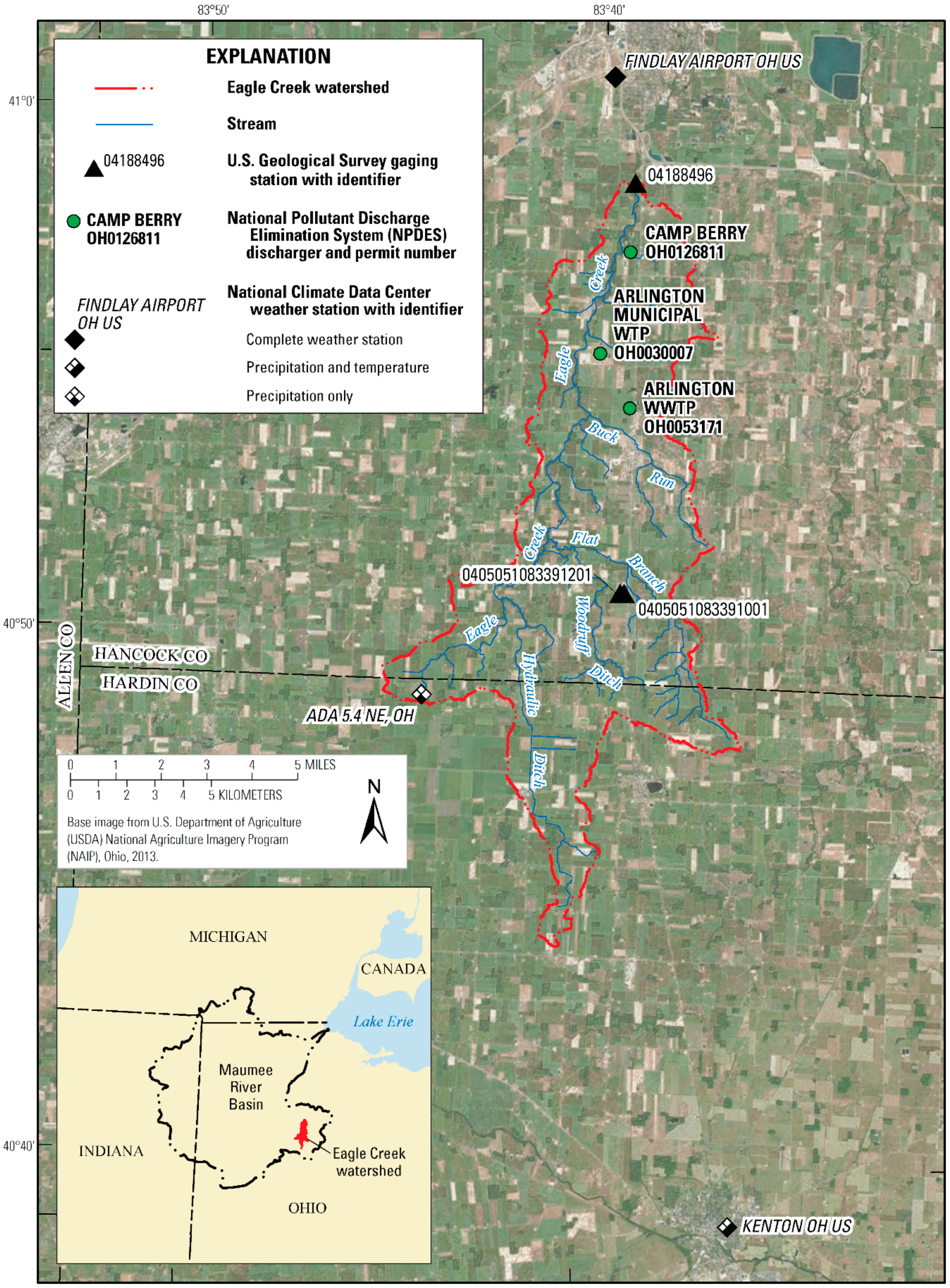
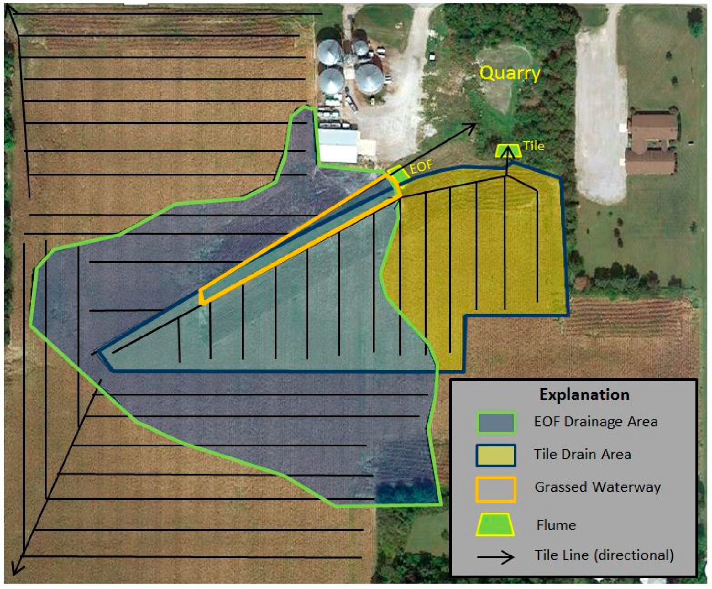
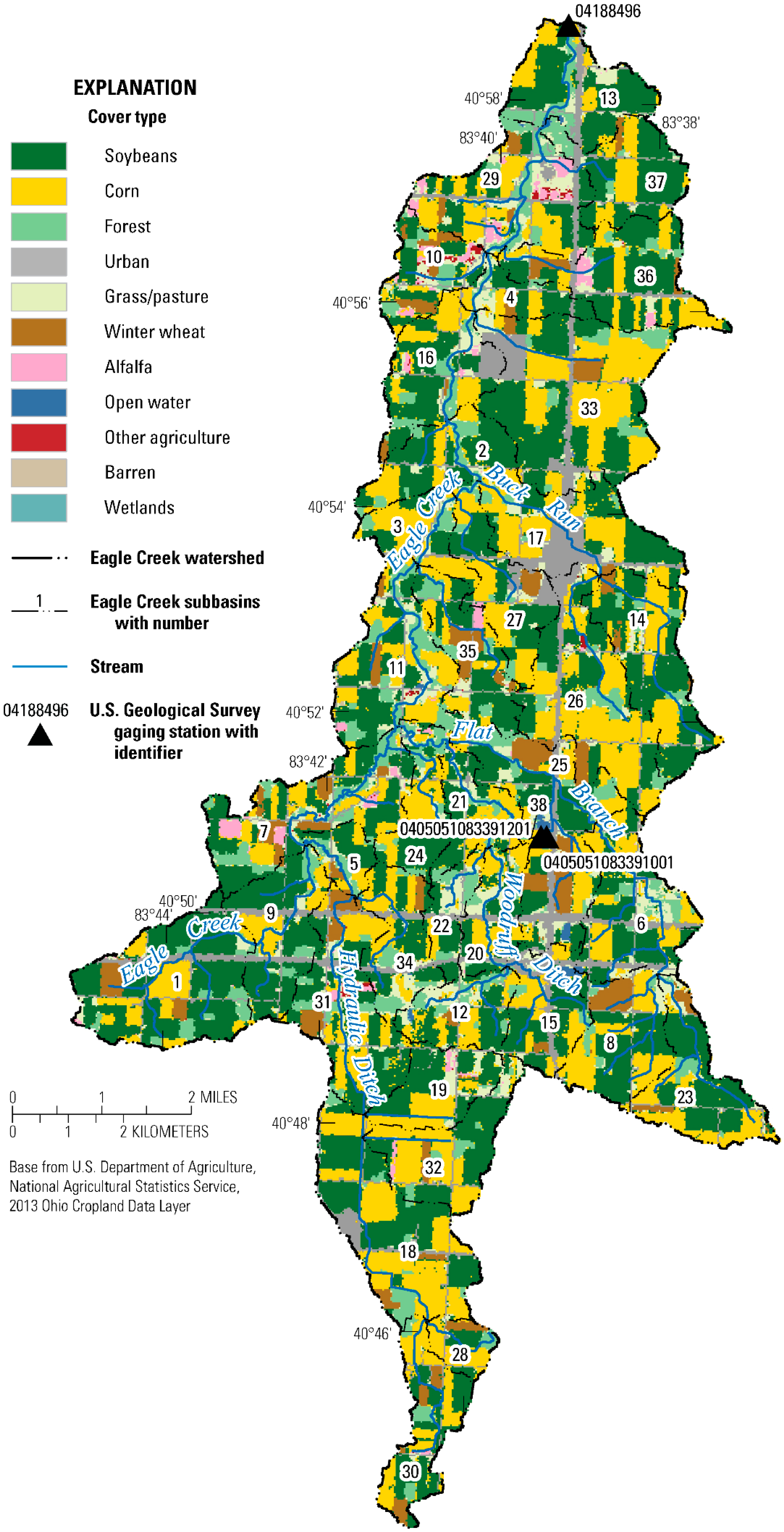
2.1. Study Watershed

The Maumee River basin is located in northwestern Ohio, northeastern Indiana, and southeastern Michigan. Within the Maumee River Basin, the focus of this study is Eagle Creek watershed with a 125-km² drainage area (Figure 1). It consists of two HUC12s: Upper and Lower Eagle Creek. The basin is mostly in Hancock County, Ohio, with some tributary headwaters originating further south into Hardin County in northwestern Ohio. The basin is located south of the city of Findlay and north of Kenton. The town of Arlington, Ohio, population 1455 [29], is within the watershed boundaries.

The Eagle Creek watershed is a heavily agricultural area with over 80% of its land use dedicated to agricultural production (Figure 2). Primary crops grown in this basin are corn and soybeans, with a few small animal farms. A typical rotation in the watershed is a two-year rotation of corn-soybeans, where no-till is performed prior to soybean planting, the result of sediment conservation efforts years ago. A growing number of producers—15% of the agricultural fields within the Eagle Creek watershed (Matt Heitkamp, NRCS, oral communication, 2014)—are on a five-year corn-soybeans-corn-soybeans-winter wheat rotation, where winter wheat is used as a cover crop. The 2013 Cropland Data Layer (CDL) of the USDA National Agricultural Statistics Service (NASS) estimated that there is 10% forest, 8% developed, and 7% pasture in the watershed [30].

The predominant soil orders are mollisols and alfisols, and the Soil Survey Geographic Database (SSURGO) estimates the basin has 99% somewhat poorly to poorly drained soils [31]. Soils have up to five layers and a depth of up to 2.030 m. The land lays very flat with little relief within the entire basin, with an estimated 1.8% slope and 61 m of relief from the National Elevation Dataset [32]. It is estimated that 97% of the historic wetlands in the basin have been removed [33]. Over 90% of the basin is presumed to use tile drains to reduce the water table during the growing season, and there are an estimated 107.5 km of tile drainage lines in the basin [34]. Streams in the Eagle Creek watershed have much lower than average base flow compared with other streams of the Maumee River watershed [35], and several streams become intermittent during the summer months. Many of the streams in the basin have been flow modified for agricultural purposes [36]. This area is highly conducive to flooding during heavy or long duration precipitation events [37]. This basin has a temperate climate, and the area receives approximately 859 mm of rainfall annually and an average of 559 mm of snowfall from November through April [38].

A USGS gaging station, (USGS 04188496 Eagle Creek above Findlay, OH, USA, hereinafter referred to as the HUC12 outlet), is located on Eagle Creek 7.6 km south of downtown Findlay. The stream corridor has an average 30.5-m riparian buffer on each side of the stream.

The EOF study area is located 22.5 km south of Findlay, Ohio (Figure 3) on a private field. The EOF drainage area was determined with a topographic survey. The study site is located on a row-crop parcel that rotates biennially between corn and soybeans. This parcel of land has gentle slopes with a 2.1 m elevation change from the highest point in the field to the entrance of the flume. The field naturally slopes inwards, and a 10.4 m by 129.5 m (0.14 ha) grassed waterway was built to drain the field. The grassed waterway has a slope of 0.82% and is made up of mostly thick grass. Because of its low-lying nature, it was more conducive to receiving water than the rest of the field and was a good location for the monitoring equipment.

USGS installed a monitoring site (0405051083391201, hereinafter referred to as EOF site) on this field for observing nutrient loads in surface runoff. The EOF monitoring site monitors a 3.5-ha field that drains through a 0.7-m H-flume. The H-Flume is flanked on either side by a treated plywood wingwall buried 0.3 m below the surface and supported on each side by an earthen dam which is planted and covered with the same grass as the swale. The wingwalls protrude 0.7 m out of the ground and are even with the top of the flume. This setup constricts the water to ensure all EOF runoff passes through the flume.

Collocated with this site, a subsurface-tile drain flow (0405051083391001, hereinafter referred to as tile site) was also monitored. The tile site monitored an estimated 2.07 ha subsurface area that drains into a tile line and through a 60-degree trapezoidal flume. The drainage area contributing to the tile drain was delineated using a tile map provided by the producer after new tile lines were installed in 2012. The tile drainage area partially overlapped the EOF drainage area (Figure 3). Approximately 60% of the EOF drainage area (blue area) was drained by the monitored tile drainage area (yellow area). The remaining 40% of the EOF drainage area was drained by other tile lines (not monitored) that flow either to the northwest or the southwest. See Supplementary Materials A, Section 1 for more information on data collection.

2.2. Model Development

SWAT was selected for the present study because of its ability to simulate different agricultural management practices needed to meet the study objectives. ArcSWAT 2012 (Revision 665b) for ArcGIS10.2 Geographic Information System interface [39] was specifically modified for this project where DRP in tile drainage (TVAP) is printed to the hydrologic response unit and subbasin output (output.hru and output.sub, respectively). This allowed the model to be calibrated with DRP measured in the tile drainage. Model inputs were described in Merriman [40].

This model used the field-scale methodology, described in companion study Merriman et al. [41], except for the differences noted below and in Supplementary Materials A. In this study, the predefined watershed boundary and stream option in the ArcSWAT interface was used to input processed National Hydrography Dataset Plus (NHDPlus) [42] scale subbasins and stream network obtained from a WLEB study developed by Texas A&M University [43]. The NHDPlus data are very detailed data which consist of NHDPlus (Version 2) streams and catchments at a scale of 1:100,000. The final delineation resulted in 39 subbasins (Figure 2). The drainage areas of the EOF (determined by survey) and tile sites (determined by tile map) (Figure 3) were merged into the NHDPlus-derived subbasins as subbasins 38 and 39, respectively. Since these subbasins overlap (Figure 3), acreage equivalent to the overlapping area was subtracted from an adjacent subbasin in its input *.sub file to ensure acreage was not double modeled. In the Eagle Creek watershed, the USDA Farm Service Agency Common Land Unit (CLU) layer [44], which was received through a Memorandum of Understanding (MOU) with NRCS described in the next section, outlined 2083 farm fields. The U.S. Fish and Wildlife Service National Wetlands Inventory wetland geospatial data layer [45] was overlaid to incorporate 225 individual wetlands and ponds, which constituted 135 ha. HRU thresholds for land use, soils, and slope were set to zero to keep the field boundaries as delineated [46]. The final number of HRUs was 2816.

2.3. Best Management Practice Implementation

Management operations were defined from interviews with local conservation agents (Megan Burgess and Matt Heitkamp, USDA-NRCS, oral communication, 2014). The majority rotation (an estimated 85% of the agricultural land) was a 2-year corn-soybean rotation (

Table 1. Two-year corn and soybean conventional and cover crop rotations in the Eagle Creek watershed, Ohio Soil and Water Assessment Tool (SWAT) model.

Rotation	Conventional		Cover Crop		Fertilizer
Year	Date	Operation	Date	Operation	Application Rate
1	24 April	Field Cultivator	20 April	Field Cultivator	-
1	1 May	Plant corn	29 April	Plant corn	-
1	3 June	Fertilizer application	1 June	Fertilizer application	220 kg ha−1 Ammonia
1	18 October	Harvest and Kill	18 October	Harvest and Kill	-
1	24 October	No-tillage	25 October	No-Tillage	-
1	-	-	30 October	Plant cereal rye	-
2	-	-	22 April	Kill cereal rye	-
2	-	-	28 April	Field Cultivator	-
2	15 May	Plant soybeans	15 May	Plant soybeans	-
2	10 October	Harvest and Kill	18 October	Harvest and Kill	-
2	29 October	Fertilizer application	29 October	Fertilizer application	168 kg ha−1 11-52-0 *
2	30 October	Deep Ripper	2 November	Deep Ripper	-

Note: * Fertilizer application rates and fertilizer content in percent N-P-K.

). A field was started on either corn or soybeans based on the CDL 2013 category used to define the majority land use for that field (i.e., corn fields for 2013 started on the corn year of the rotation, whereas soybean fields for 2013 started on the soybean year of the rotation). The remaining agricultural fields, approximately 15% of the agricultural land, used a 5-year rotation of corn-soy-corn-soy-winter wheat (

Table 2. Five-year corn, soybean, corn, soybean winter wheat (CR) and cover crop and crop rotations (CC + CR) rotations in the Eagle Creek watershed, Ohio SWAT model.

Rotation	CR		CC + CR		Fertilizer
Year	Date	Operation	Date	Operation	Application Rate
1	-	-	15 April	Kill cereal rye	-
1	24 April	Field Cultivator	24 April	Field Cultivator	-
1	1 May	Plant corn	28 April	Plant corn	-
1	1 June	Fertilizer application	1 June	Fertilizer application	220 kg ha−1 Ammonia
1	18 October	Harvest and Kill	18 October	Harvest and Kill	-
1	24 October	Generic No-Tillage	24 October	Generic No-Tillage	-
2	15 May	Plant soybeans	1 May	Plant soybeans	-
2	10 October	Harvest and Kill	10 October	Harvest and Kill	-
2	29 October	Fertilizer application	22 October	Fertilizer application	168 kg ha−1 11-52-0 *
2	30 October	Deep Ripper	24 October	Deep Ripper	-
3	24 April	Field Cultivator	24 April	Field Cultivator	-
3	1 May	Plant corn	28 April	Plant corn	-
3	3 June	Fertilizer application	3 June	Fertilizer application	220 kg ha−1 Ammonia
3	18 October	Harvest and Kill	18 October	Harvest and Kill	-
3	24 October	Generic No-Tillage	24 October	Generic No-Tillage	-
4	15 May	Plant soybeans	1 May	Plant soybeans	-
4	1 October	Harvest and Kill	1 October	Harvest and Kill	-
4	2 October	Fertilizer application	2 October	Fertilizer application	50.5 kg ha−1 Elem P 11.3 kg ha−1 Elem N
4	3 October	Generic No-Tillage	3 October	Generic No-Tillage	-
4	5 October	Plant winter wheat	5 October	Plant winter wheat	-
5	15 July	Harvest and Kill	15 July	Harvest and Kill	-
5	25 October	Chisel Plow Gt 15 ft	24 August	Generic No-Tillage	-
5	-	-	22 October	Plant cereal rye	-

Note: * Fertilizer application rates and fertilizer content in percent N-P-K.

); this 5-year rotation was applied to fields where the majority CDL 2013 land use was winter wheat. Fertilizer amounts were derived from the Tri-State Fertilizer Recommendations [47].

In order to describe the spatial variability of BMPs throughout this watershed, USGS entered into a MOU with USDA-NRCS to access the National Conservation Planning (NCP) database, which manages the repository of NRCS-funded BMPs throughout the US. In order to maintain USDA-NRCS privacy requirements, no information regarding any producer’s identity was received. NCP practice information, including practice name, scheduled implementation date, certification date, funding source, location (GIS coordinates), and quantity (i.e., number of acres), was received for 2649 individual practices of 53 different USDA-NRCS practices in the Eagle Creek watershed. Practices ranged in scheduled implementation dates from 2005 to 2018. The certification date indicated the date that a BMP was approved as “on the ground” and entered into the NCP database. These practices are hereinafter referred to as “Applied” practices. Other practices scheduled for implementation, but not yet certified as implemented, are hereinafter referred to as “Planned” practices. While there were multiple funding sources, this effort only distinguished between those practices categorized as GLRI funded and the remaining as nonGLRI funded (see Supplementary Materials A, Section 5 for further information on BMP selection).

NCP BMPs were implemented on HRUs based on their spatial location, implementation status (Applied or Planned), and funding source (GLRI or nonGLRI). Point locations of BMPs were spatially joined to the field-based HRUs.

Hardin and Hancock Counties, Ohio NRCS conservation agents provided information on how BMPs were implemented in the Eagle Creek watershed (

Table 3. Best management practices in Eagle Creek watershed, Ohio and representation in SWAT.

Short ID	USDA-NRCS Code *	NRCS Practice	Representation in SWAT
CRP	327	Conservation Cover	Established switch grass permanently
CR	328	Conservation Crop Rotation	Added winter wheat on 5th year of rotation
CC	340	Cover Crop	Cover crop of cereal rye planted after tillage following corn harvest
UW	647 645	Early Successional Habitat Development/Management Upland Wildlife Habitat Management	Established rangeland permanently
FS	393	Filter Strip	Used SWAT filter strip option (ops file) Area derived from GIS
GW	412	Grassed Waterway	Used SWAT grassed waterway option (ops file) Length and width derived with GIS. Slope and depth assumed as defaults
NMP	590	Nutrient Management Plan	Reduced P containing fertilizer applications by 10%
PG	528	Prescribed Grazing	Method for beef cattle described in text
RT	345	Residue Management, Reduced Till	Moldboard replaced with conservation tillage in corn years. no-till in soybean year CN2.mgt-2; BIOMIX.mgt = 0.4; OV_N.hru = 0.2
NT	329 329A 329B	Residue Management, No-Till/OR Strip TillOR Mulch Till	Moldboard replaced with no-tillage operation in corn years. no-till in soybean year CN2.mgt-5; BIOMIX.mgt = 0.5; OV_N.hru = 0.3

Notes: NRCS = Natural Resources Conservation Service; P = phosphorus; SWAT = Soil and Water Assessment Tool; * USDA-NRCS BMPs conform to standards that are available online [50].

). These assumptions were meant to reflect the general operations of the BMPs in the Eagle Creek watershed. Assumptions regarding tillage management practices (reduced till (RT) and no-till (NT) were modified from Arabi et al. [48]. Locations of grassed waterways (GW) and filter strips (FS) were included with the NCP data, and their length and width were derived from Google Earth. GW depth and slope were assumed as 0.25 m and 0.012, respectively, based on NRCS conservation agent input about averages in the watershed. GW and FS were simulated using the *.ops files and the Vegetative Filter Strip Model (VFSMOD) developed for SWAT [49]. Nutrient management plan (NMP) reduced any P-containing fertilizers by 10%. Conservation crop rotation (CR) switched the field from the conventional 2-year corn-soybean rotation to the 5-year rotation which contained winter wheat (Table 2). For the cover crop (CC) BMP, cereal rye was planted following the harvest of corn in late October and was harvested prior to the planting of soybeans in April (Table 1). Conservation cover (CRP) and Upland Wildlife Habitat Management (UW) established permanent, continuously growing grasslands, simulated with switchgrass and clover, respectively, as recommended by NRCS as typical crops used in these practices. Prescribed grazing (PG) for beef cattle was simulated with the grazing operation, using a before and after approach whenever PG was implemented on a field. The following changes were made from pre- to post- PG installation: Number of consecutive grazing days (GRZ_DAYS) from 250 days to 200 days and dry weight of biomass consumed daily (BIO_EAT) from 8 kg ha⁻¹ to 5 kg ha⁻¹. The dry weight of biomass trampled daily (BIO_TRMP) was set to 3 kg ha⁻¹, minimum plant biomass required for grazing to occur (BIO_MIN) was set to 1.5 kg ha⁻¹, and dry weight of manure deposited daily (MANURE_KG) was set to 3 kg ha⁻¹ for both pre- and post-PG. Implementation of PG in SWAT is meant to represent the overall reduction in number of days spent by cattle in a single field, rather than the rotating cattle from pasture to pasture which local conservation agents indicated was occurring in this area.

2.4. Scenarios

In Eagle Creek watershed, BMPs were Applied in 12.9% of the watershed according to the NCP database (

Table 4. BMP implementation scenarios investigated with the Eagle Creek watershed SWAT model, Ohio.

Modeled Scenarios	Practices per Scenario		Fields with NCP BMPs (BMP Count)	Area of NCP BMPs (ha)	Percent of Watershed with BMPs (%)
Baseline	-		0 fields (0 BMPs)	0	0
Applied GLRI BMPs	CC on 26 fields	NT on two fields	42 fields (50 BMPs)	363.1	2.8
	CR on 10 fields	one GW
	NMP on nine fields
All Applied BMPs (GLRI + nonGLRI BMPs)	CC on 41 fields	NT on 109 fields	275 fields (560 BMPs)	1679.6	12.9
	CR on 162 fields	RT on 38 fields
	CRP on 51 fields	19 GW
	NMP on 100 fields	25 FS
	PG on 15 fields	14 UW
All Applied + Planned GLRI BMPs	CC on 41 fields	NT on 109 fields	277 fields (564 BMPs)	1699.8	13.0
	CRP on 51 fields	RT on 38 fields
	CR on 164 fields	19 GW
	NMP on 102 fields	25 FS
	PG on 15 fields	14 UW
All Contracted BMPs (All Applied and Planned: GLRI + nonGLRI BMPs)	CC on 41 fields	NT on 114 fields	298 fields (623 BMPs)	1827.7	14.0
	CRP on 61 fields	RT on 41 fields
	CR on 171 fields	45 GW
	NMP on 108 fields	27 FS
	PG on 15 fields	14 UW
Low	CC on 41 fields	NT on 294 fields	477 fields (1163 BMPs)	3038.2	23.3
	CRP on 61 fields	RT on 41 fields
	CR on 351 fields	45 GW
	NMP on 288 fields	27 FS
	PG on 15 fields	14 UW
Medium	CC on 41 fields	NT on 619 fields	825 fields (2173 BMPs)	5961.4	45.8
	CRP on 61 fields	RT on 40 fields
	CR on 675 fields	82 GW
	NMP on 613 fields	27 FS
	PG on 15 fields	14 UW
High	CC on 961 fields	NT on 1538 fields	1,729 fields (5855 BMPs)	9946.5	76.3
	CRP on 61 fields	RT on 40 fields
	CR on 1594 fields	84 GW
	NMP on 1532 fields	40 FS
	PG on 15 fields	14 UW

Notes: BMPs = best management practices; CC = cover crops; CRP = conservation cover; CR = crop rotation; FS = filter strip; GLRI = Great Lakes Restoration Initiative; GW = grassed waterway; NCP = USDA Natural Resources Conservation Service National Conservation Planning database; NMP = nutrient management plan; NT = no-tillage; PG = prescribed grazing; RT = reduced tillage; UW = upland wildlife habitat management.

). The majority of NCP BMPs are funded by programs other than GLRI; fields with GLRI funded BMPs (Applied and Planned) make up 2.8% of Eagle Creek watershed. CR was the most popular BMP, which was applied in 9% of the Eagle Creek watershed. The majority of fields had multiple BMPs applied. The most commonly applied BMP combination was a trio of BMPs: CR, a tillage practice (NT or RT), and NMP. NTs is used in this paper to denote NT prior to soybean planting as seen in the conventional rotation.

Several conservation practice scenarios were simulated based on the NCP data (Table 4). In addition to these scenarios, three hypothetical BMP scenarios (Low, Medium, and High BMP implementation) were also simulated. Hypothetical scenarios were developed in consultation with local NRCS personnel to determine what practices would be of the most interest to local producers. The Low and Medium scenarios randomly applied a trio of BMPs (CR + NMP + NT) to 25% and 50% of the remaining agricultural fields, respectively. In the Medium scenario, a GW was added to one field in every subbasin in the model, excluding subbasins 38 and 39. The High scenario applied the BMP trio and added CC to all remaining agricultural HRUs without a BMP in the model. An FS was added to any HRU where the TP was greater than 5 kg ha⁻¹. These scenarios were all compared to the Baseline scenario, which did not include any BMPs from the NCP database. To simulate BMP performance under a range of precipitation and flow conditions, all scenarios were simulated for a 10-year period (2005 to 2014), after a 5-year warm-up period. Loads computed for the Baseline scenario were used to calculate percent reduction against loads from the other scenarios. As scenarios progressed (Table 4 and

Table 5. BMP or BMP combinations by scenario investigated with the Eagle Creek watershed SWAT model, Ohio.

Scenario	Applied GLRI	All Applied	All Applied and Planned GLRI	All Contracted BMPs	Low Scenario	Medium Scenario	High Scenario
BMP or BMP Combination	(Hectares)
CC	175.1	103.0	103.0	72.3	72.3	72.3	72.3
CC + CR + NMP + NT	-	126.6	126.6	114.5	114.5	114.5	4100.7
CC + CR + NMP + NT + FS	-	14.7	14.7	14.7	14.7	14.7	59.7
CC + CR + NMP + NT + FS + GW	-	-	-	-	-	-	17.9
CC + CR + NMP + NT + GW	-	39.9	39.9	52.0	52.0	52.0	191.0
CC + CR + NMP + RT	-	14.5	39.9	39.9	39.9	39.9	39.9
CC + CR + NT	-	56.7	56.7	31.2	31.2	31.2	31.2
CC + CR + NT + GW	-	-	-	25.6	25.6	25.6	25.6
CC + CR + RT	-	25.4	-	-	-	-	-
CC + GW	-	-	-	30.7	30.7	30.7	30.7
CC + NMP	53.3	-	-	-	-	-	-
CC + RT	25.4	-	-	-	-	-	-
CR	61.5	92.2	112.4	66.1	66.1	66.1	66.1
CR + GW	-	-	-	39.3	39.3	39.3	39.3
CR + NMP	-	0.6	0.6	0.6	0.6	0.6	0.6
CR + NMP + NT	-	253.9	253.9	261.5	261.5	252.5	252.5
CR + NMP + NT + FS	-	47.0	47.0	49.4	49.4	49.4	49.4
CR + NMP + NT + FS + GW	-	-	-	2.8	2.8	2.8	2.8
CR + NMP + NT + GW	-	22.4	22.4	35.0	35.0	44.1	44.1
CR + NMP + NTs	-	-	-	-	1210.5	3384.1	3382.9
CR + NMP + NTs + GW	-	-	-	-	13.3	276.1	276.1
CR + NMP + RT	-	240.4	240.4	240.2	240.2	208.8	208.8
CR + NMP + RT + GW	-	-	-	29.7	29.7	61.0	61.0
CR + NT	-	161.4	161.4	137.6	137.6	137.6	137.6
CR + NT + GW	-	12.7	12.7	36.6	36.6	36.6	36.6
CR + RT	-	71.7	71.7	16.2	16.2	15.0	15.0
CR + RT + GW	-	-	-	55.4	55.4	55.4	55.4
CRP	-	86.6	86.6	96.9	96.9	96.9	95.2
CRP + FS	-	43.9	43.9	43.9	43.9	43.9	45.6
FS	-	54.0	54.0	54.0	54.0	54.0	8.9
FS + GW	-	17.9	17.9	17.9	17.9	17.9	-
GW	3.0	96.1	96.1	181.0	167.7	655.8	516.8
NMP	34.7	15.3	15.3	-	-	-	-
NMP + NT	10.1	-	-	-	-	-	-
PG	-	66.6	66.6	66.6	66.6	66.6	10.6
PG + FS	-	-	-	-	-	-	2.7
PG + GW	-	-	-	-	-	-	53.2
UW	-	14.6	14.6	14.6	14.6	14.6	13.3
UW + FS	-	1.4	1.4	1.4	1.4	1.4	2.7
Total	363.1	1679.6	1699.8	1827.7	3038.2	5961.4	9946.5

Notes: BMP = best management practice; CC = cover crops; CRP = conservation cover; CR = crop rotation; FS = filter strip; GLRI = Great Lakes Restoration Initiative; GW = grassed waterway; NCP = USDA Natural Resources Conservation Service National Conservation Planning database; NMP = nutrient management plan; NT = no-tillage; NTs = no-tillage following the corn harvest prior to soybean planting; PG = prescribed grazing; RT = reduced tillage; UW = upland wildlife habitat management.

), more practices may be added, or an existing practice may be enhanced (i.e., from RT to NT), but once a BMP was installed in a field it was not removed. BMPs were maintained during the entire simulation period; they were not implemented on specific calendar dates. BMP scenarios were created to quantify the impact of these BMPs over a long-term period with similar climate to 2005 to 2014; these simulations are not intended to quantify effect GLRI had on loads in any given year.

2.5. Calibration and Validation Procedure

Hydrologic calibration of the SWAT model was performed by simulating exports from the watershed from water year (WY, the 12-month period October 1, for any given year through September 30, of the following year) 2007 through WY2014 with a 5-year warmup period. The calibration period of the water quality components was WY2013 to WY2014. The model was calibrated with the All Applied scenario, which incorporated all BMPs that were certified in the NCP as Applied as of February 2015 (see Supplementary Materials A, Section 5 on BMPs). Subsequently, the calibration would best reflect the applied BMPs installed in the Eagle Creek watershed during the modeling period. The validation period was WY2015 to WY2016. Various simulated and monitored hydrological and water-quality components were compared at the EOF, tile, and the HUC12 outlet sites. EOF and tile monitoring data were compared to the SWAT results in surface runoff or subsurface flow, respectively, using the model results found in the output.sub file for subbasins 38 (EOF) and 39 (tile). At the EOF location where surface runoff was monitored, surface runoff, sediment yield (overland erosion), DRP, TP, NO₃-N, and TN (all in surface runoff) were compared, whereas at the tile site, tile flow, tile NO₃-N, and DRP in the tile output were compared. At the HUC12 outlet, flow, sediment, NO₃-N, DRP, TN, and TP were compared.

The quantitative statistics to evaluate model performance at the HUC12 outlet, as recommended by Moriasi et al. [51], applied in this study were Nash–Sutcliffe simulation efficiency (NSE), the coefficient of determination (R²), and percentage bias (PBIAS). NSE ranges from −∞ to 1, where an optimal model fit to the observed data is equal to 1. NSE values between 0.75 and 1 indicates a very good model fit, 0.65–0.75 is good, 0.50–0.65 is satisfactory, and <0.5 is unsatisfactory. NSE is the most accepted and implemented statistical standard for the evaluation of performance in watershed modeling [16,52,53]. R² ranges from 0 to 1 and higher values demonstrate a better fit of the simulated data to the observed data. Values of R² above 0.5 are considered satisfactory. PBIAS is used to assess the average tendency of system response. The optimal value of PBIAS is 0.0%, where absolute values of PBIAS <10%, <15%, and <25% indicate a very good model fit for streamflow, sediment, and nutrients, respectively, 10–15%, 15–30%, and 25–40% indicate good, 15–25%, 30–55%, and 40–70% indicate satisfactory, and >25%, >55%, and >70% indicate unsatisfactory. Positive values of PBIAS indicate the model is underestimating bias and negative values indicate the model is overestimating bias [54]. In addition to quantitative statistics, visual comparisons between observed and simulated hydrographs were evaluated and the simulation was considered satisfactory when the shape (peaks and base flow) of observed and predicted hydrographs were reasonably similar. Additionally, several soft calibration constraints were considered and are discussed in the following section.

2.6. Calibration and Validation Procedure

For multiscale calibration in watershed models, the ASABE Engineering Standards Engineering Practice 621 [24] recommends starting calibration at the smaller scale and then calibrating at the larger scale. Calibration was first performed at the EOF and tile sites. Parameters from Daggupati et al. [43] and Yen et al. [55] were used as a starting point for calibration and adjusted or modified to suit the simulated conditions in the study watershed. Detailed management data, as implemented by the producer from 2012 to 2016, were available and used for management in subbasins 38 and 39. Hydrology and water-quality were calibrated for best performance at a monthly time step at the HUC12 outlet. These were evaluated using quantitative statistics and visual comparisons of hydrographs. Parameter adjustments were made using a combination of autocalibration with SWAT-CUP [56] and manual trial-and-error calibration until the overall hydrological budgets (tile flow, surface runoff, ground water, etc.), quantitative statistics, and visual comparisons of hydrographs between observed and simulated at the HUC12 outlet were reasonable. This study incorporated the tile monitoring data into calibration to ensure the correct portion of the water balance was being simulated through the subsurface pathway. Tile drain systems are designed to remove excess field water and lower water tables to allow timely field tillage and planting and reduce crop stresses. Hydrology is substantially changed when intensive tile drainage is implemented throughout a watershed, as in this Eagle Creek watershed, and tile drainage can increase the speed and quantity of nutrient export [57,58]. In the Eagle Creek, Ohio SWAT model tile drains were represented by the “newer” tile drainage algorithm (ITDRN = 1) based on the Hooghoudt and Kirkham equations [59]. Specific records of tile locations were not available in the watershed at this time; however, local conservation agents (Matt Heitkamp, USDA-NRCS, oral communication, 2014) estimated that tile drainage was implemented in the vast majority of agricultural fields in the study watershed. Accordingly, tile drainage was simulated in agricultural fields with poorly drained or very poorly drained soils (hydrologic soil groups of C or D).

Tile drainage parameters effective radius of drains (RE) and distance between two tiles (SDRAIN) were set to 20 mm and 20,000 mm, respectively, as in Boles et al. [60]. Boles et al. [60] and Sui and Frankenburger [61] have indicated the depth to impervious layer (DEP_IMP) for tiled HRUs should be set to just beneath the depth to the tile drains (DDRAIN) to ensure tile flow was not artificially impeded. DEP_IMP for nontiled HRUs was set to 6000 mm. Pump capacity (PC) was set to 0 to indicate that all tile drainage occurred due to gravity flow.

Initially, the model was not producing tile flow in the winter months, whereas the monitored data demonstrated tile flow during the same period. Tile flow will not occur in SWAT when the first soil layer is frozen, which occurs when simulated soil temperatures are less than 0 °C [19]. In SWAT, the daily soil temperatures are calculated empirically as a function of several variables, including the previous day’s soil temperature at certain depth, the average annual air temperature, the current day’s soil-surface temperature, and vertical position in the soil profile. The SWAT-simulated, winter soil temperatures prevented tile flow even with an adjusted lag factor that controlled the influence of the previous day’s temperature and current day’s [62]. In this study, all negative air temperatures were converted to 0 °C within the simulation period and the snowfall temperature (SFTMP) was set to 0.5 °C. Thus, SWAT accounted any precipitation as snow when the air temperature was below 0.5 °C. This approach allowed accurate simulation of snowfall while the soil temperature remained close enough to observed soil temperature to allow simulated tile flow. This modification facilitated simulating the winter tile flow reasonably well. Temperature modifications increased annual average tile flow, while decreasing annual average surface runoff and overall water yield. Impact was also seen in soil-water content and percolation during winter months and the groundwater storage. For more information on the impact of changing the input air temperature, see Supplementary Materials C.

After the winter tile hydrology was improved, calibration continued at the EOF and tile sites to develop the correct quantity and timing of subsurface flow. Like in Boles et al. [60], a decrease in curve number (CN2) was required to induce tile flow. This change subsequently decreased surface runoff and increased tile flow, but a decreased CN2 could result in lower storm peaks and possibly reduce the simulated surface transport of nutrients. Moriasi et al. [59] accounted for this problem with the introduction of a soil moisture retention parameter (R2ADJ) to account for increased soil water content in tile drained soils, which is used when ICN = 0. Setting R2ADJ = 0 sets CN2 equal to field capacity (this is the default), and R2ADJ = 1 calculates CN2 at saturation [27]. A value of R2ADJ between 0 and 1, allows CN2 to be calculated at a range of soil water capacities which is more realistic for heavily drained fields rather than at field capacity or at saturation. Here R2ADJ, was set at 0.1 to indicate that some amount of soil-water is present through simulation. Finally, LATKSATF, which controls subsurface and surface flow portioning [27,60], was set to its maximum value to increase the simulated tile flow hydrograph. Some of these parameters may have a larger effect at the watershed scale, rather than at the field scale. After hydrology calibration, sediment was calibrated to account for overland erosion and sediment yield at the EOF outlet (SYLD from output.sub for subbasin 38). It was important to have sediment processes well-calibrated because these processes will alter the performance of organic P and TP transport substantially. Manning’s N (OV_N) was slightly adjusted and the quantitative statistics and hydrographs between observed and simulated sediment yields at the EOF site were compared. The channel-related parameters were adjusted after extrapolating the EOF related parameters throughout the watershed. In-stream sediment routing was performed by using the simplified Bagnold Equation. SWAT-CUP was used to adjust the channel-related parameters CH_N2, SPCON, and SPEXP (Table S3) using NSE as the objective function in multiple iterations with 500 simulation runs.

Nutrient calibration was the final step in calibration. By default, the SWAT model sets the initial concentration of the potentially soluble phosphorus (SOL_LABP.chm) in all soil layers to 5 mg kg⁻¹. The soil test P (STP) laboratory assessment provided by the producer at the EOF site was 20 mg kg⁻¹. While it was recognized that this value can vary by farm field, 20 mg kg⁻¹ was used throughout the watershed to set SOL_LABP. Maximum crack volume of soil profile (SOL_CRK) was an important parameter to control simulated DRP at the tile site, with simulated TVAP increasing with SOL_CRK. Channel-related parameters and the organic nutrient concentrations (SOL_ORGP and SOL_ORGN; Table S3) were determined with SWAT-CUP [56], using the same objective function and number of runs as described for sediment parameters, with separate simulations for N and P constituents. The remaining parameters affecting nutrients were controlled at the watershed scale, including nitrogen and P uptake rates (N_UPDIS and P_UPDIS). In order to ensure that real world conditions were simulated reasonably well, soft calibration constraints were used; these are discussed in the next section.

Model results are not publicly available or have limited availability owing to privacy restrictions due to the MOU between USGS and NRCS. This model contains sensitive data: The GIS coordinates and quantity of BMPs derived from the USDA-NRCS NCP database, contact Jon Hortness (USGS; [email protected]) for more information.

3. Results

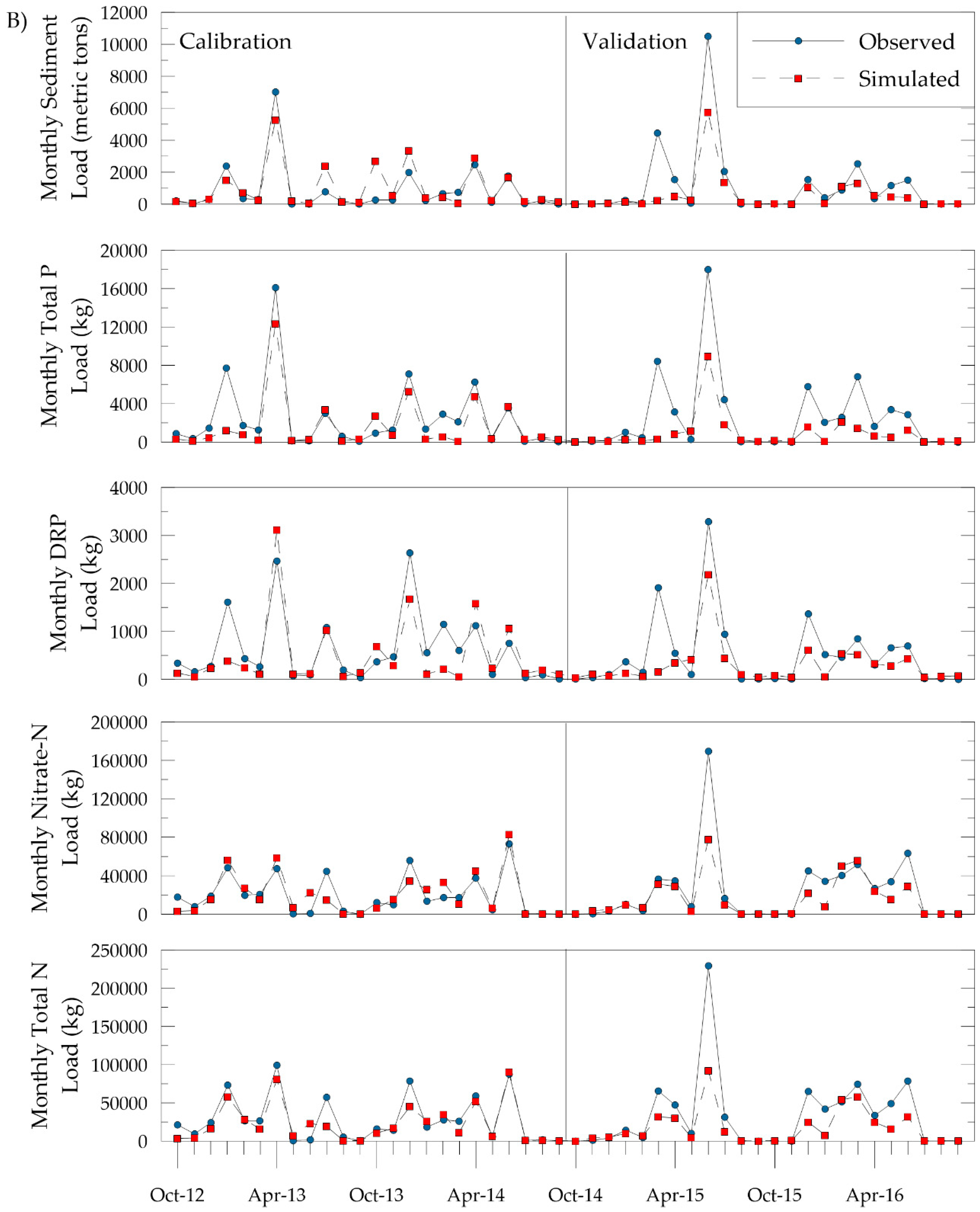
3.1. Calibration and Validation

Soft constraints as recommended in Arnold et al. [63] were also considered. First, the tile flow should be no more than 25% of the rainfall [64]; the simulated tile flow was 18.6% of the rainfall. The simulated base flow to total flow ratio was 16%, similar to the 25% reported by Schiefer [35] for a slightly larger Eagle Creek watershed drainage area in the 1940s and 1950s. The simulated denitrification rate was 15.4 kg N ha⁻¹, which is less than the 50 kg N ha⁻¹ constraint [65]. The ratio of nitrate contributed from tile flow (TNO3) to total nitrate was 72%, slightly more than the recommended two-thirds which was based on a single field study in Iowa [64]. Variation is expected to be present in fields in other areas. Crop yield calibration was also performed, see Section 3.1.3.

At the HUC12 outlet, simulated flow performed better in summer and fall during low flow periods than during high flow in winter and spring months (Figure 4). Some high winter flows were undersimulated or produced a single peak while there were dual peaks in the hydrograph. In the calibration period, flow, sediment, NO₃-N, and TP had a good NSE rating (0.65–0.75); DRP and TN were satisfactory (0.5–0.65) (

Table 6. Calibration and validation summary statistics at the monthly time step for Eagle Creek watershed, Ohio SWAT model.

Constituent	NSE	PBIAS	R2	NSE	PBIAS	R2
	Calibration WY2013–WY2014			Validation WY2015–WY2016
Eagle Creek Outlet (USGS 04188496)
Flow *	0.69	−4.59	0.70	0.64	40.79	0.83
Sediment	0.72	−19.17	0.73	0.62	50.30	0.84
DRP	0.61	18.96	0.67	0.57	41.88	0.72
TP	0.74	34.30	0.82	0.41	63.68	0.76
NO3-N	0.68	−3.50	0.73	0.63	33.72	0.79
TN	0.63	−14.22	0.76	0.53	47.77	0.84
EOF (USGS 0405051083391201)
surface runoff	0.33	26.97	0.41	−0.36	−8.81	0.36
Sediment	0.66	−18.94	0.67	0.73	−22.47	0.79
DRP	−24.91	−338.83	0.42	−7.31	−134.83	0.07
TP	0.41	−58.13	0.62	−0.80	−72.58	0.66
NO3-N	−0.20	86.11	0.16	−0.10	89.88	0.00
TN	0.04	80.93	0.78	0.15	78.60	0.64
Tile Drain (USGS 0405051083391001)
tile flow	0.34	−46.53	0.86	0.78	14.53	0.79
DRP	0.05	−45.92	0.28	0.14	45.97	0.23
NO3-N	−0.78	78.84	0.28	−0.21	84.63	0.03

Note: * Flow calibration at the HUC12 outlet period of record was 2007–2014. For the Eagle Creek outlet, green shading indicates very good rating, yellow shading indicates good rating, and grey shading indicates satisfactory rating according to ratings in Moriasi et al. [51]. DRP = dissolved reactive phosphorus; NO3-N = nitrate-nitrogen; NSE = Nash–Sutcliffe simulation efficiency; PBIAS = percentage bias; R² = coefficient of determination; TP = total phosphorus; TN = total nitrogen; USGS = U.S. Geological Survey; WY = water year, the 12-month period 1 October–30 September designated by the calendar year in which it ends.

). Sediment and TP had a good PBIAS rating and all other constituents had a very good PBIAS rating. All values of R² were satisfactory (≥0.5) for the calibration period.

The model performed with a satisfactory NSE rating (NSE ≥ 0.5) for all constituents except TP during the validation period (WY2015–WY2016), and all constituents had a satisfactory R² (≥0.5). All constituents were underestimated in the validation period, especially during large flows in June 2015, when heavy flooding occurred in the area [66,67]. While flow had satisfactory ratings for NSE and R², flow had an unsatisfactory PBIAS rating (≥25%) due to undersimulating several large peaks. The remaining constituents had at least a satisfactory or better PBIAS rating (±40%–±70% for nutrients; ±30%–±55% for sediment). The model had a better fit to the observed data in WY2016 than WY2015.

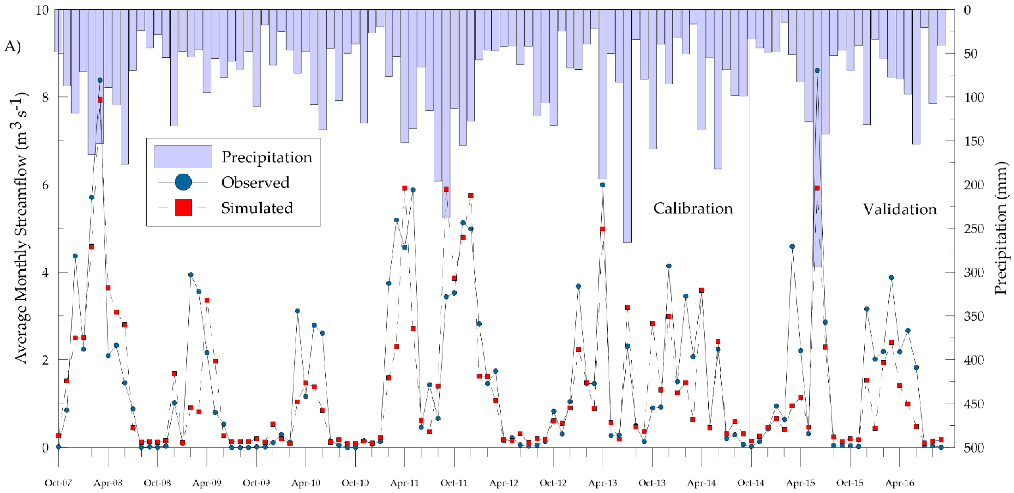
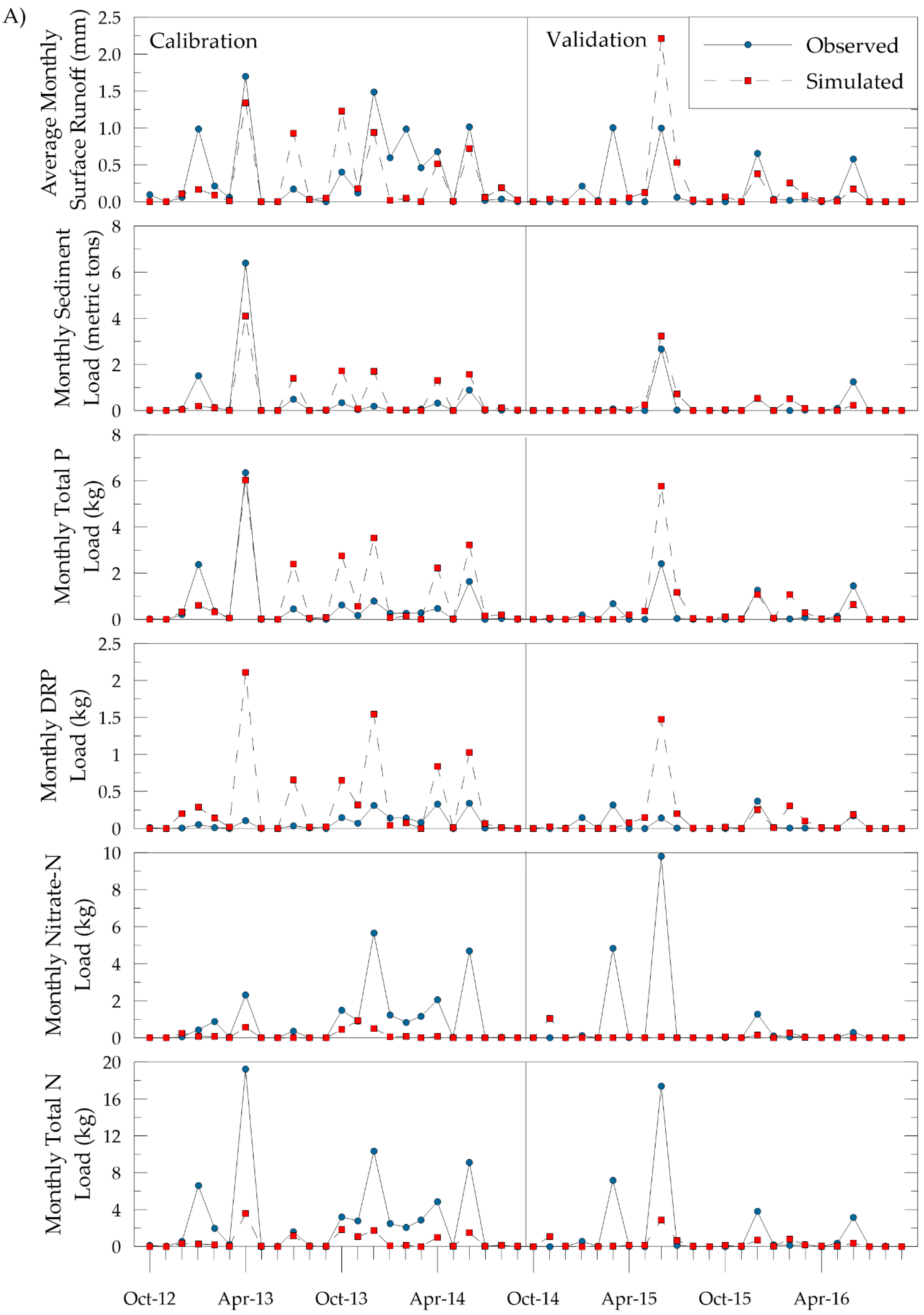
3.1.1. EOF Calibration and Validation

The EOF outlet at subbasin 38 was calibrated for several constituents generated through overland processes at the surface runoff outlet (using the results in output.sub for subbasin 38): Surface runoff (SURQ), overland sediment (SYLD), overland DRP (SOLP), overland NO₃ (NSURQ), overland TP (SOLP + ORGP + SEDP), and overland TN (NSURQ + ORGN). Calibration was performed at the monthly timestep using visual comparisons of hydrographs (Figure 5A); quantitative statistics were provided for reference (Table 6). Monthly fluctuations seen in the observed data were generally replicated at the EOF site. Surface runoff was underpredicted during the calibration period and overpredicted during the validation period. Surface runoff was undersimulated in the calibration period (PBIAS = 26.97) and oversimulated in the validation period (PBIAS = −8.81); winter peaks were underestimated in both periods. Sediment, TP, and DRP, were oversimulated in the calibration and validation periods, while TN and NO₃-N was undersimulated in both periods. NSE and PBIAS for SYLD were in the good range for the calibration period and in the satisfactory range in the validation period; R² for SYLD, TP, and TN was rated satisfactory for the calibration and validation periods. R² and PBIAS were in the satisfactory range for TP in the calibration period.

Visually, the patterns of peaks at the daily timestep were well simulated with SWAT at the EOF site (Figure 5B). Surface runoff was undersimulated in the calibration period and over simulated in the validation period; the timing of simulated events to observed events matched well. TN and NO₃-N were undersimulated, while sediment, DRP, and TP were oversimulated.

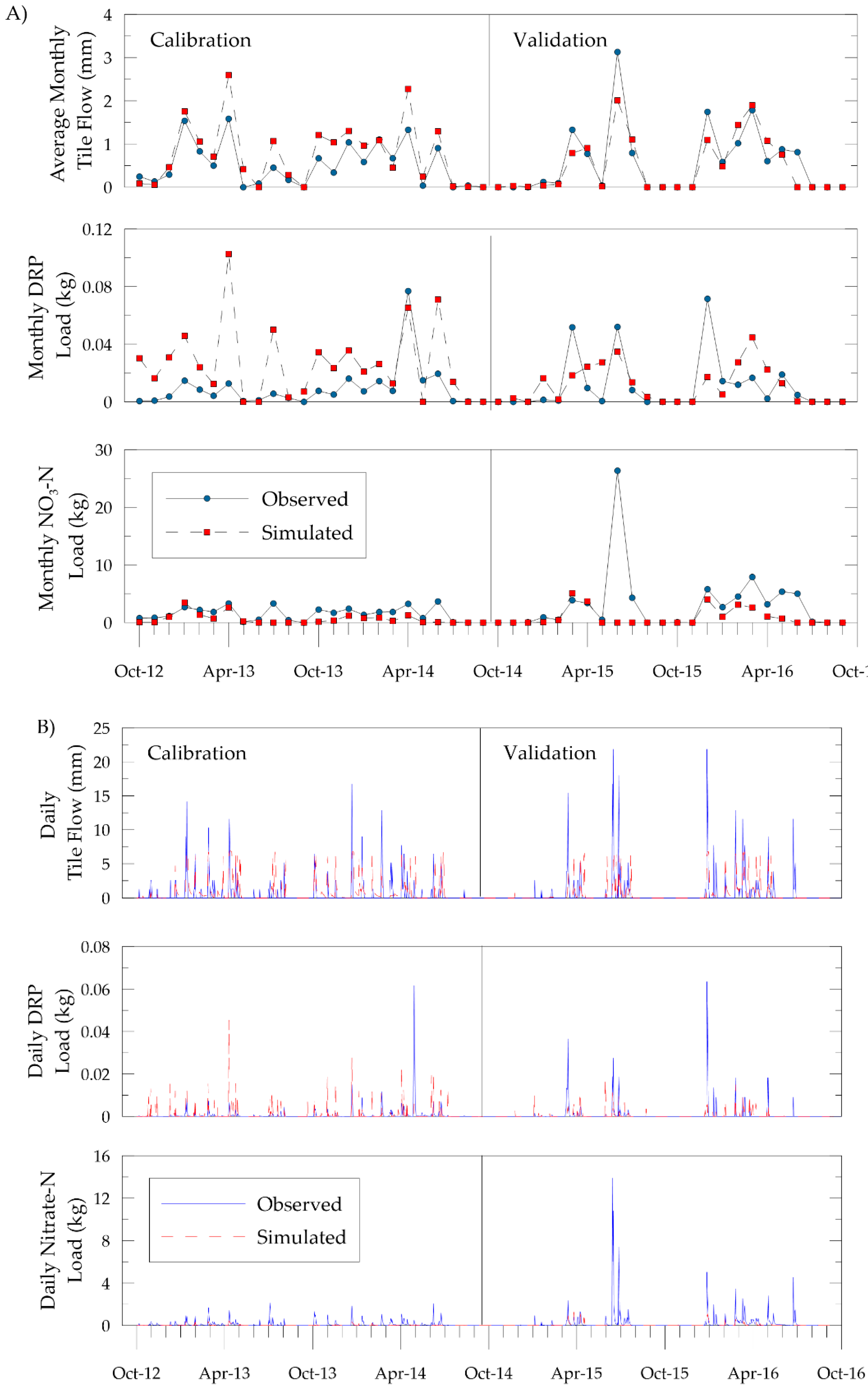
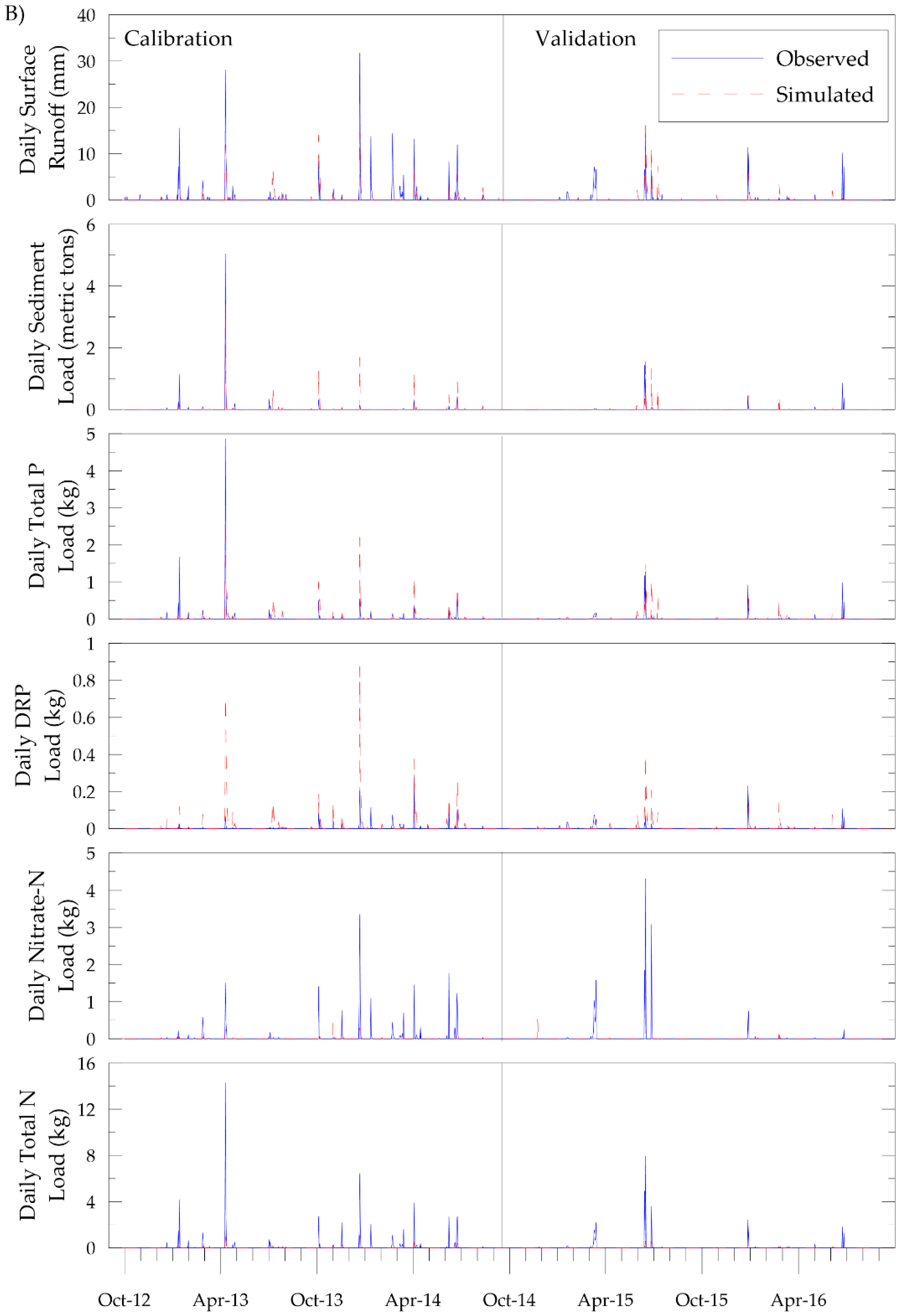
3.1.2. Tile Calibration and Validation

The measured constituents (tile flow, NO₃-N, and DRP) in tile drainage were compared to simulated tile flow (Qtile in output.sub for subbasin 39), simulated tile NO3 (TNO3 in output.sub for subbasin 39), and DRP at the tile outlet (TVAP from output.sub for subbasin 39). Simulated constituents generally followed the observed data (Figure 6). Qtile and DRP were in the satisfactory range for R² and PBAIS, respectively, in the calibration period (Table 6); however, NSE for the DRP and NO₃-N was in the unsatisfactory range for both calibration and validation periods. NSE and PBIAS for Qtile was in the very good range during the validation period. TNO3 was undersimulated in both calibration and validation periods, while Qtile and DRP were oversimulated in the calibration period and undersimulated in the validation period. TN, TP, and sediment were also measured at the tile site; however, SWAT does not simulate these components in tile drainage. Thus, calibration was only performed for the tile flow and soluble nutrients at the tile outlet.

Daily hydrographs and chemographs for the tile site are shown in Figure 6B. Daily NSE for Qtile, TNO3, and TVAP were 0.05, 0.08, and −0.67, respectively in the calibration period. In the validation period NSE was 0.28, 0.01, and 0.17 for Qtile, TNO3, and DRP, respectively. Qtile was oversimulated in both calibration and validation periods, and seemed to have a maximum of approximately 6.5 to 6.7 mm.

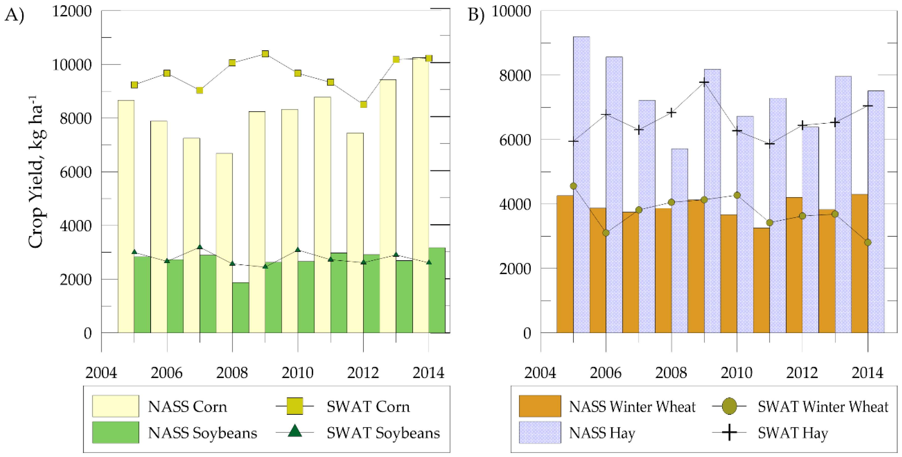
3.1.3. Crop Yield Calibration

Crop yields were compared to the four main crops (corn, soybeans, winter wheat, and hay) reported by the USDA for Hancock County, Ohio [68] over the 10-year simulation period. Simulated crop yields visually follow reported crop yields (Figure 7). Simulated crop yields overestimated the corn and soybean yields, whereas the other crop yields were underpredicted (

Table 7. Annual summary statistics from 2005 to 2014 for crop yield calibration for the Eagle Creek watershed, Ohio SWAT model.

Crop	Average Annual Crop Yield (kg ha−1)		PBIAS	R2
	Observed	Simulated	(%)
Corn	8126	9631	−11.25	0.51
Soybean	2744	2781	−1.12	0.24
Winter Wheat	3997	3752	2.68	0.01
Hay	7192	6581	7.85	0.12

Notes: PBIAS = percentage bias; R² = coefficient of determination.

). The summary statistics were well within ranges reported in other SWAT modeling projects. Srinivasan et al. [69] suggested crop yields were acceptable when the PBIAS is within ±15%, which was the case for the compared crops. N fixation from soybeans was simulated at 182.37 kg N ha⁻¹, within the range of other reported studies in the Midwest: 172–206 kg N ha⁻¹ in Illinois [70] and 100–200 kg N ha⁻¹ in Ohio [71], but was higher than the range reported for the state of Ohio (61–122 kg N ha⁻¹ [72].

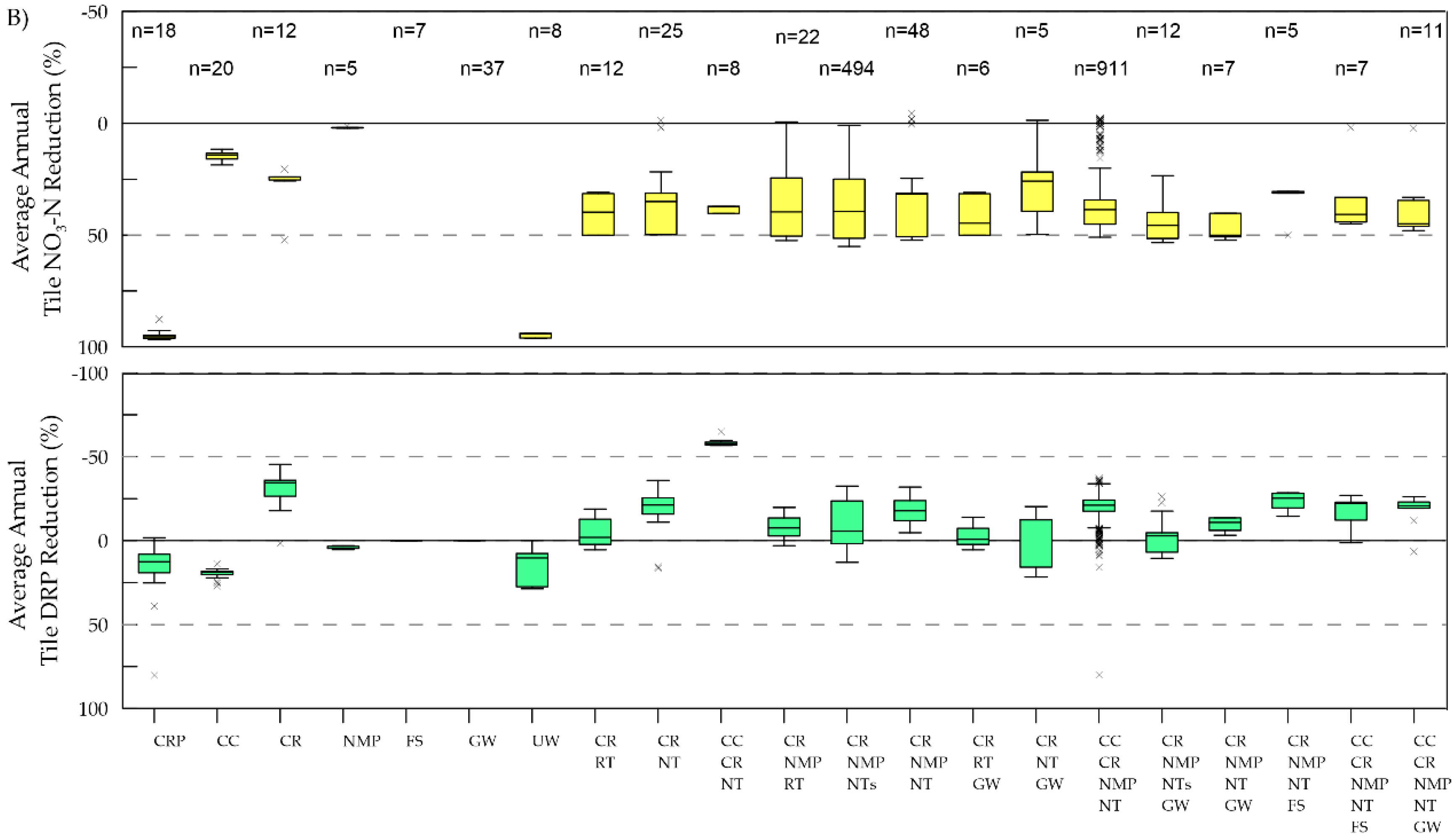
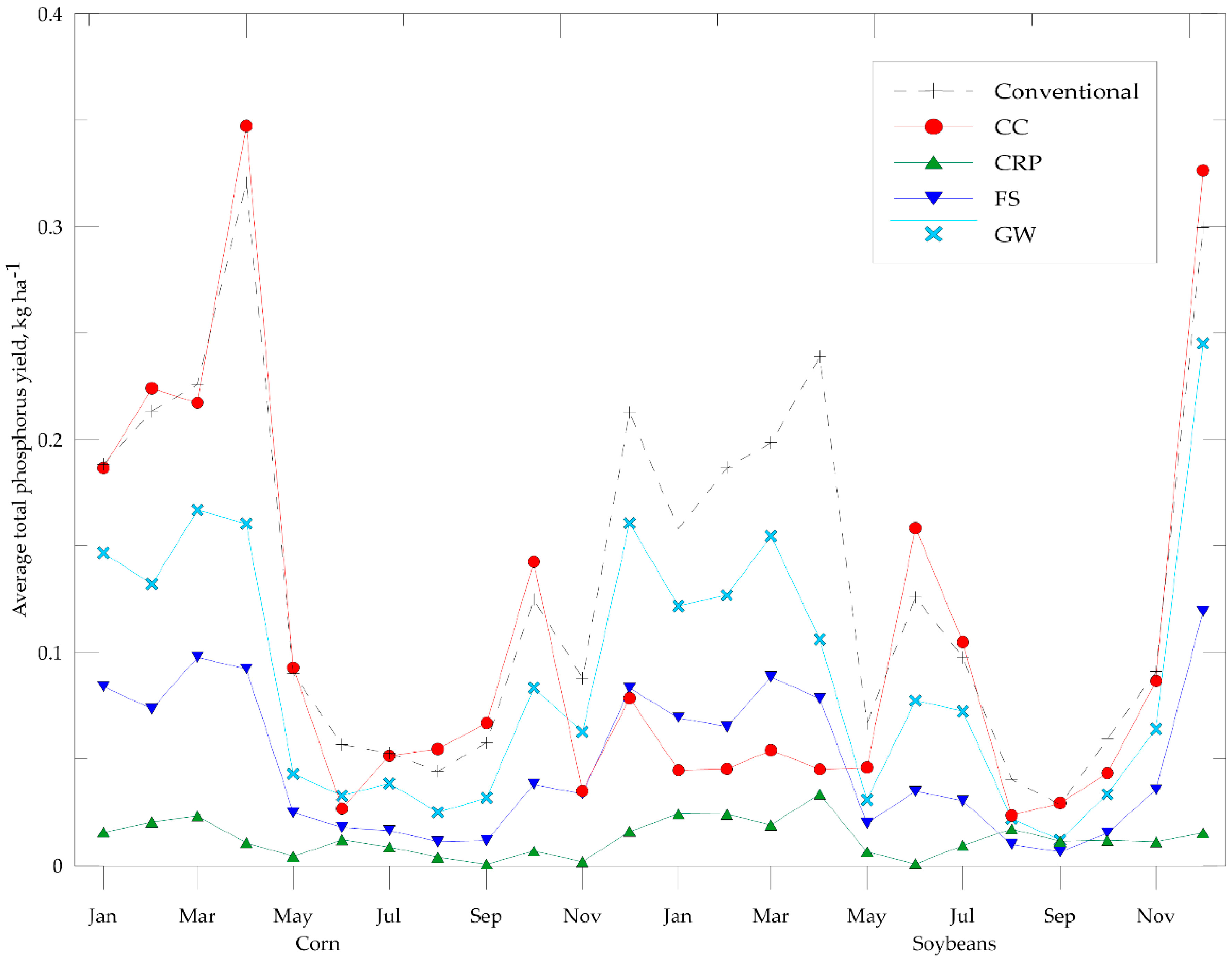
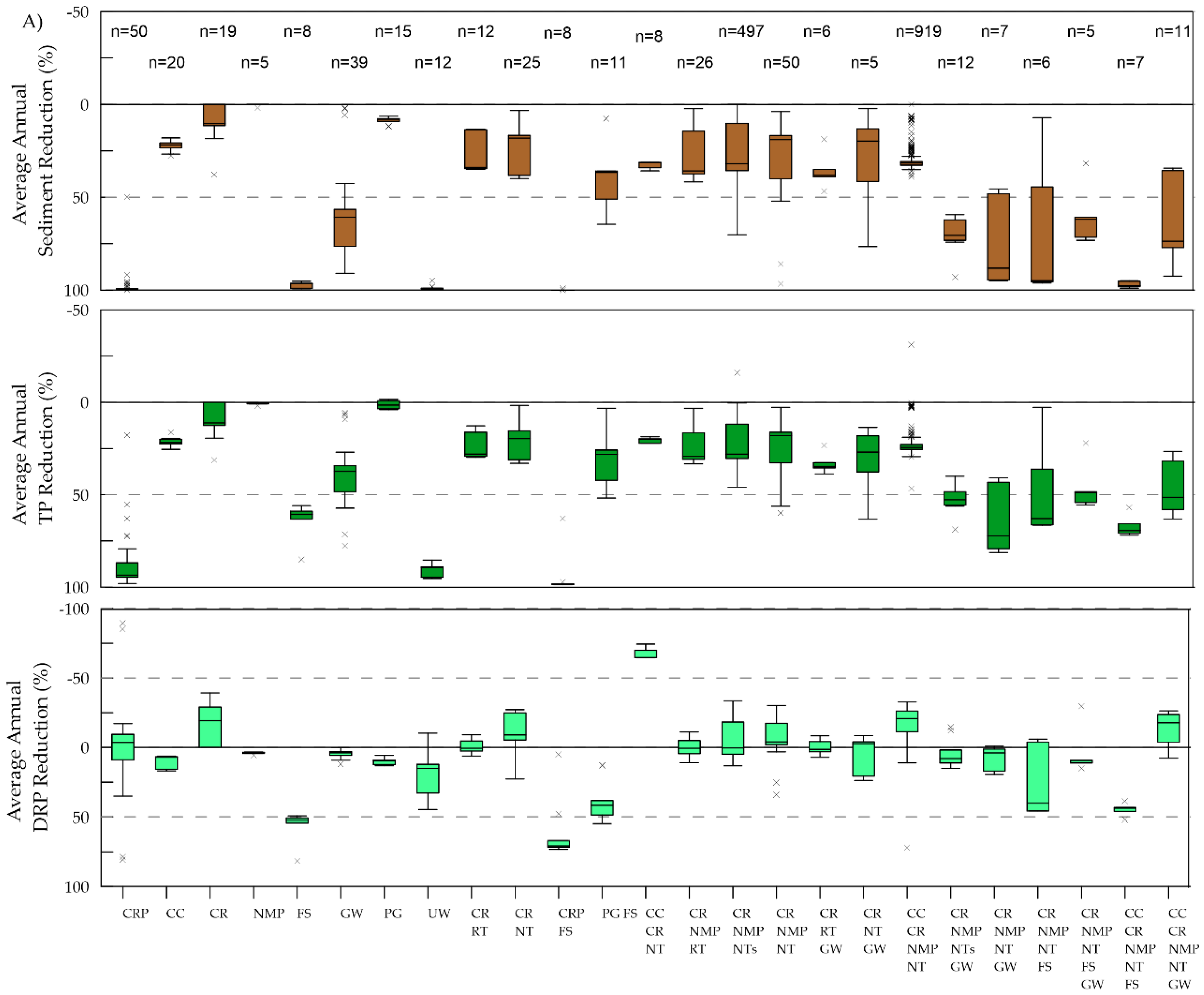
3.2. Effect of Best Management Practices at the Field-Scale

The differences in average annual losses of sediment, DRP, and TP associated with BMP implementation were computed for a 10-year period (2005–2014) and aggregated by BMP or BMP combination. There were 39 different BMPs or BMP combinations evaluated (Table 5 and

Table 8. Average annual reductions in sediment and nutrient loadings by BMP or BMP combination with the Eagle Creek watershed, Ohio SWAT model. Negative values indicate an increase in sediment or nutrients.

BMP or BMP Combination		Average Annual Reductions (%)
	n	Sediment	DRP	TP	NO3-N	TN
CC	20	22%	9%	21%	10%	12%
CC + CR + NMP + NT	919	31%	−18%	23%	37%	39%
CC + CR + NMP + NT + FS	7	97%	45%	67%	39%	43%
CC + CR + NMP + NT + FS + GW	1	99%	42%	73%	46%	49%
CC + CR + NMP + NT + GW	11	62%	−14%	45%	37%	43%
CC + CR + NMP + RT	3	41%	16%	35%	54%	56%
CC + CR + NT	8	33%	−67%	20%	36%	0%
CC + CR + NT + GW	3	39%	−69%	28%	37%	42%
CC + CR + RT	1	41%	12%	34%	53%	56%
CC + GW	1	23%	7%	27%	10%	13%
CC + NMP	4	23%	15%	23%	14%	15%
CC + RT	2	23%	10%	21%	8%	14%
CR	19	9%	−17%	9%	19%	21%
CR + GW	3	21%	−28%	22%	25%	30%
CR + NMP	1	39%	0%	33%	50%	51%
CR + NMP + NT	50	28%	−7%	23%	34%	36%
CR + NMP + NT + FS	6	72%	27%	50%	31%	36%
CR + NMP + NT + FS + GW	5	60%	3%	46%	47%	48%
CR + NMP + NT + GW	7	77%	7%	66%	46%	52%
CR + NMP + NTs	497	23%	−5%	20%	35%	0%
CR + NMP + NTs + GW	12	70%	3%	52%	41%	45%
CR + NMP + RT	26	26%	0%	23%	34%	37%
CR + NMP + RT + GW	2	54%	3%	42%	46%	52%
CR + NT	25	25%	−11%	22%	34%	36%
CR + NT + GW	5	31%	6%	32%	28%	31%
CR + RT	12	26%	−1%	23%	40%	42%
CR + RT + GW	6	36%	0%	33%	41%	44%
CRP	50	98%	2%	88%	95%	97%
CRP + FS	8	100%	60%	94%	96%	98%
FS	8	97%	56%	63%	6%	13%
FS + GW	1	99%	51%	64%	3%	9%
GW	39	60%	4%	39%	1%	9%
NMP	5	0%	4%	1%	2%	2%
NMP + NT	2	8%	−3%	3%	−3%	0%
PG	15	9%	10%	2%	0%	0%
PG + FS	11	40%	40%	31%	35%	25%
PG + GW	2	53%	49%	43%	53%	40%
UW	12	99%	18%	90%	83%	0%
UW + FS	3	100%	48%	92%	72%	0%

Notes: BMP = best management practice; CC = cover crops; CRP = conservation cover; CR = crop rotation; DRP = dissolved reactive phosphorus; FS = filter strip; GLRI = Great Lakes Restoration Initiative; GW = grassed waterway; n = number of HRUs with BMP combination implemented; NCP = USDA Natural Resources Conservation Service National Conservation Planning database; NMP = nutrient management plan; NO3-N = nitrate-nitrogen; NT = no-tillage; NTs = no-tillage following the corn harvest prior to soybean planting; PG = prescribed grazing; RT = reduced tillage; TP = total phosphorus; TN = total nitrogen; UW = upland wildlife habitat management.

). The combined field-level results for all scenarios, where BMP or BMP combination was applied to five or more fields, are shown in Figure 8. Variability in field reductions ranged from −90 to 100% (Figure 8A) and tile reductions ranged from −65 to 97% (Figure 8B). Generally, BMPs reduced sediment and TP in the BMP combinations, but DRP was increased in some BMP combinations. The maximum average reduction in sediment (100%), TP (94%), and DRP (60%) yields occurred with the combination of CRP + FS. FS alone reduced sediment, TP, and DRP by 97%, 63%, and 56% on average, respectively. When FS was added to any other combination it further reduced sediment, TP, and DRP by an average of 31%, 22%, and 43%, respectively. Application of GW to fields reduced losses of sediment 60%, TP 39%, and DRP 4% on average, whereas the addition of a GW to other BMP combinations reduced sediment, TP, and DRP by an average of 20%, 17%, and 5%, in addition to the reduction already seen with the outstanding BMPs, respectively. CR decreased sediment (average of 9%) and TP (average of 9%) loads, but CR increased DRP (average of 17%). CC reduced sediment, TP, and DRP by an average of 22%, 21%, and 9%, respectively. Approximately half of the BMP combinations that had included CR had average increases in DRP yields (indicated by negative reductions in Table 8 and Figure 8). The combination of CC + CR + NMP + NT, which was applied to all fields in the High scenario, had average reductions in sediment, TP, and DRP of 31%, 23%, and −18%, respectively. Use of NMPs had limited average reductions when simulated as the only BMP on a field (sediment 0%, TP 1%, and DRP 4%), yet when it was applied in conjunction with other BMPs average reductions increased (sediment 16%, TP 12%, and DRP 5%).

Tillage practices, such as NT and RT, were not simulated without another BMP. NT was already incorporated into the conventional rotation (Table 1) after the corn harvest; therefore, only minor additional effects were expected to occur from an addition of either tillage practice after the soybean harvest. RT reduced DRP and TP more that NT, because NT does not mix fertilizers through the soil [73]. This was also reflected by RT having greater reductions in tile DRP than NT (Figure 8B).

Reductions of soluble nutrients in tile drainage due to BMP and BMP combination are compared in Figure 8B. Tile NO₃-N loads were reduced by most BMPs and BMP combinations, where only a few outlying fields observed an increase in tile NO₃-N. CRP and UW caused the greatest reductions in tile NO₃-N. Contrastingly, most BMPs or BMP combinations caused increases in tile DRP loads. Only CC, NMP, UW and combinations of CRP reduced tile DRP loads. The remaining BMPs or BMP combinations either contained NT, RT, or CR. These practices also caused increases in surface DRP runoff at the field (Figure 8A).

Surface runoff and sediment and nutrient yields were also compared at a monthly time step. The most surface runoff occurred in the following order: April, March, and January. In Figure 9, results of the conventional rotation were compared with select single BMP rotations; these were averaged monthly TP yields from conventional and BMP rotations. In the CC rotation, TP loads were reduced during the winter through early spring while the cereal rye crop was growing (after the corn harvest in mid-October). Most of this load reduction came in the particulate P (PP) form. Average TP loads were similar the rest of the year after CC harvest in April. FS and GW have a fraction of the TP yields compared to the conventional rotation on all months.

Not shown on Figure 9, CR generally decreased TP yield in soybean years compared to corn years, with the exception of the month of April when DRP and TP increased in the soybean year and decreased in corn-growing years. After the winter wheat harvest in the fifth year of the CR rotation, the field was bare from mid-July to the beginning of April. This lack of vegetation caused a decrease in plant uptake of phosphorus (PUP) and an increase in DRP runoff and TVAP in the fifth year. The increases in TP in February and April of the corn growing years occurred after winter wheat harvest with larger precipitation events that occurred in those months.

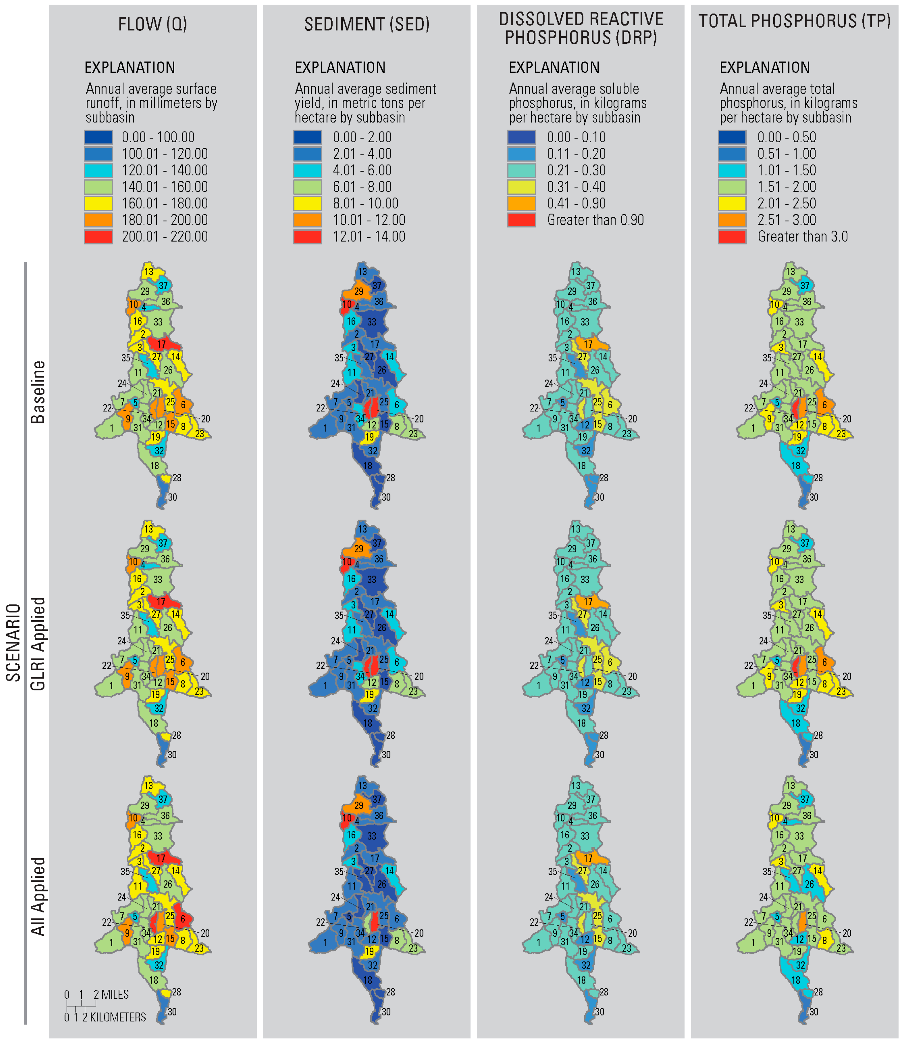
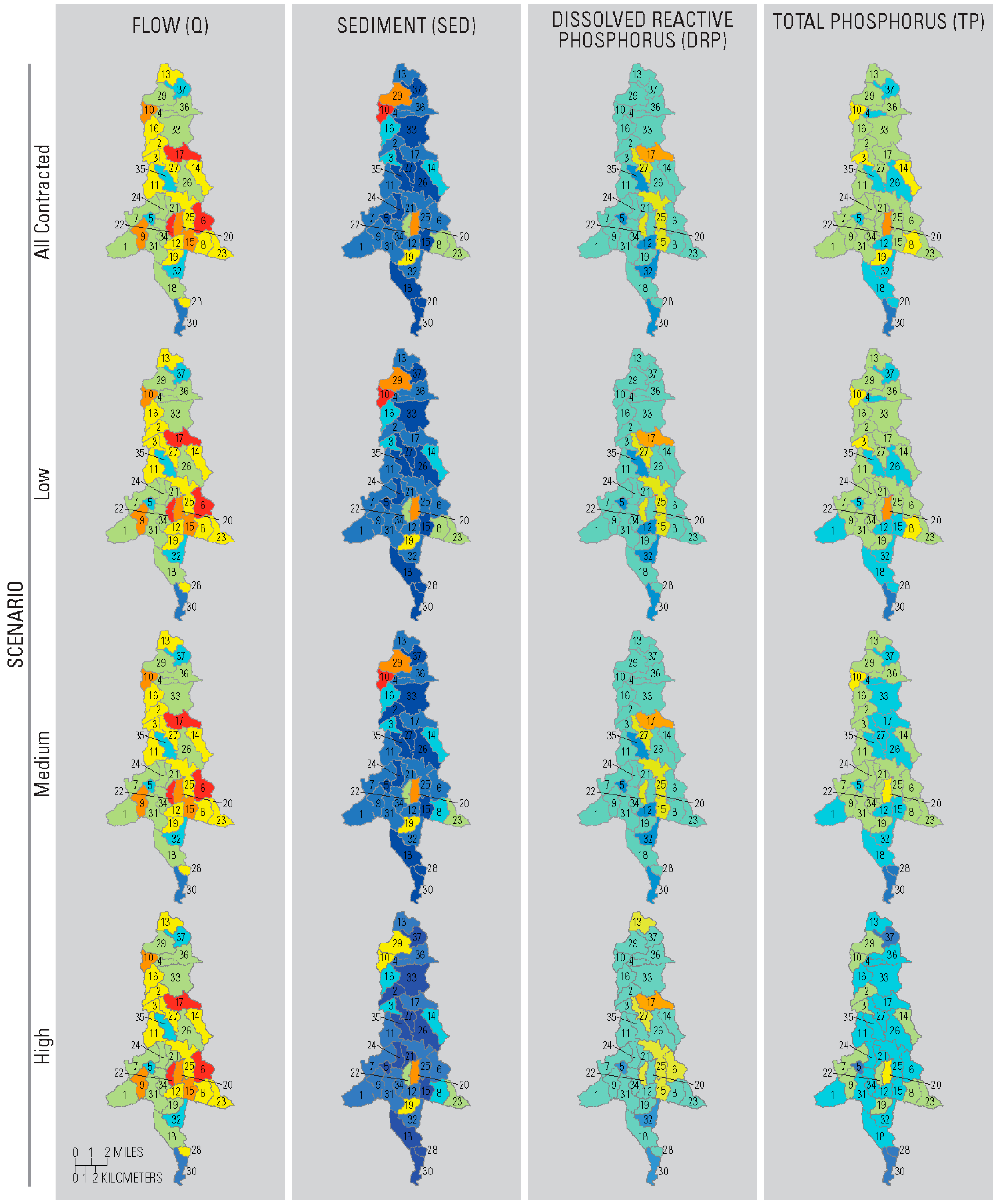
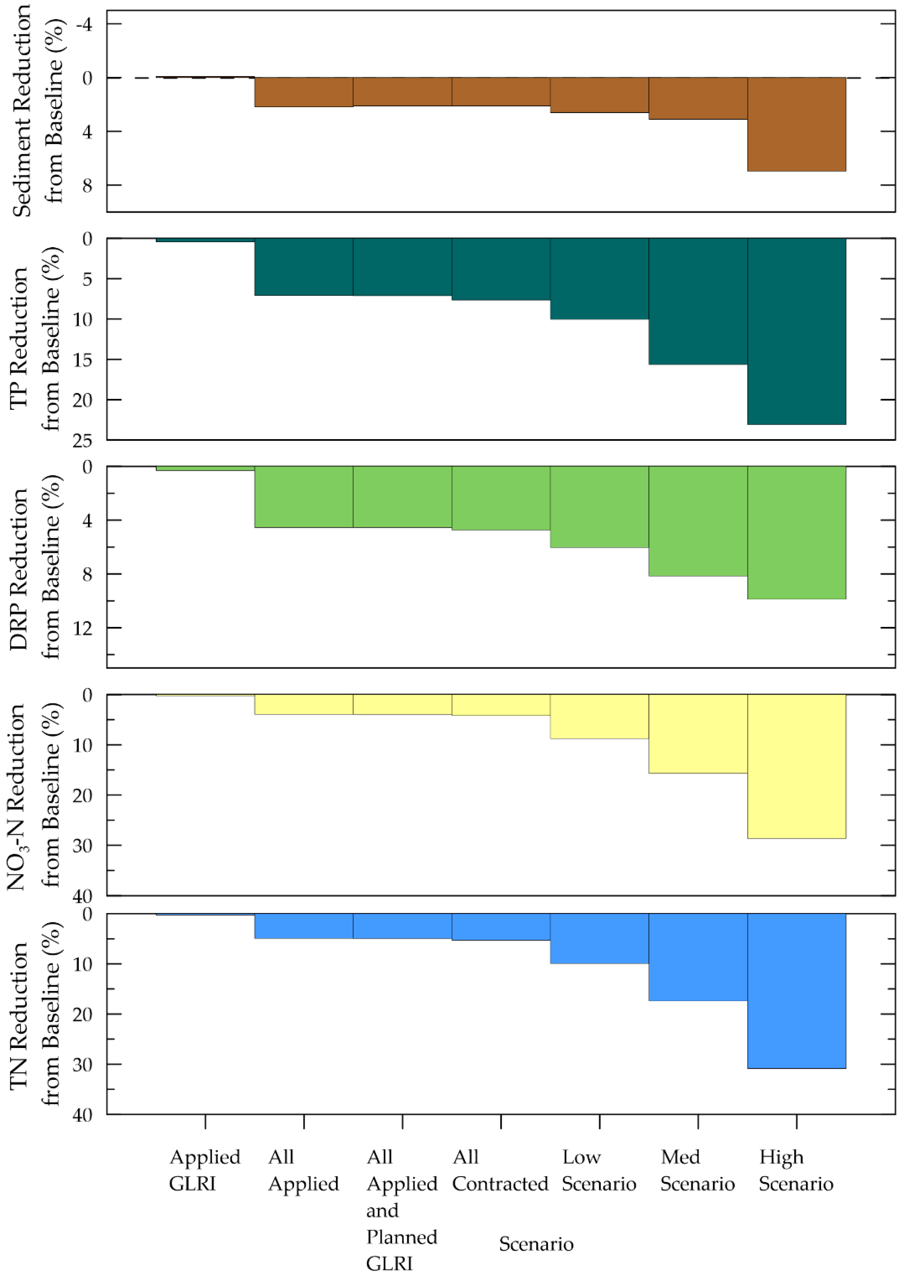
3.3. Effect of Best Management Practices at the Watershed-Scale

Modeling scenarios were run on an annual basis from 2000 to 2014, including a 5-year warm-up period. Generally, as scenarios increase the number and area where BMPs were applied, greater reductions were seen in nutrient loads at the HUC12 outlet (Figure 10). Sediment loads were nearly unchanged (increased −0.1%) in the Applied GLRI scenario but decreased in the other scenarios. Minor changes in sediment and nutrient loads were found between All Applied, All Applied + Planned, and All Contracted scenarios, because the area of BMP implementation increased only slightly from 12.9%, 13.0% and 14.0%, respectively. In the All Applied scenario, which represents the NCP BMPs that were certified as implemented, watershed-scale reductions for sediment, TP, and DRP were approximately 2%, 7% and 4.5%.

Hypothetical scenarios decreased sediment and nutrient loads. The greatest reductions were seen for TN, NO₃-N, and TP. The Low and Medium scenarios applied the BMP combination of CR + NMP + NT to 25% and 50% of the remaining agricultural areas in Eagle Creek watershed without a BMP. The High scenario added the combination CC + CR + NMP + NT to the remaining fields without a BMP. This combination was slightly more effective at reducing TP (23%) than CR + NMP + NT used in the Low and Medium scenarios (20%). For both combinations, the majority of the TP reductions occurred in PP loss from surface runoff. Both combinations showed a general increase in DRP from both surface runoff and through tile drainage on the majority of fields. DRP reductions at the watershed scale were very similar in the Medium and High scenarios, 8.2% and 9.9%, respectively, even though approximately 4000 ha of BMPs were added to the Medium scenario to create the High scenario.

Yields from the contributing land uses to streams are shown in

Table 9. Average annual yields by land use in the All Contracted scenario investigated with the Eagle Creek watershed, Ohio SWAT model.

Land Use	Hectares	Sediment Yield (t ha−1)	TP Yield (kg ha−1)	DRP Yield (kg ha−1)	NO3-N Yield (kg ha−1)	TN Yield (kg ha−1)
Row crops *	9726	1.56	1.44	0.18	1.81	4.27
Pasture	666	43.48	5.05	0.21	0.11	4.16
Grazing **	67	71.02	8.18	0.44	5.08	13.48
Urban	1075	0.40	1.37	1.11	44.24	44.58
Forest	1404	0.01	0.03	0.02	0.01	0.01
Water/Wetlands	89	0.00	0.01	0.01	0.00	0.00
Barren	3	11.66	3.36	0.19	0.00	1.04

Notes: * Row crops include fields with any combination of corn, soybeans, winter wheat and/or cereal rye; ** Grazing fields were identified by the placement of prescribed grazing BMPs; DRP = dissolved reactive phosphorus; NO3-N = nitrate-nitrogen; TP = total phosphorus; TN = total nitrogen.

. Attenuation due to stream processes was not considered in this table. Grazing land use, which occurred on 28 fields (defined by the placement of PG BMPs), had the largest average annual yields for sediment and TP, followed by Pasture land use which was simulated using SWAT defaults. Row Crops make up approximately 75% of the Eagle Creek watershed, and account for the majority of TP and DRP loads in the All Contracted scenario. The highest DRP, NO₃-N, and TN yields were contributed from urban land uses which are composed of rural homesteads, roads, and the small town of Arlington, Ohio. The high NO₃-N and TN yields were due to applying the urban areas defaults, where autofertilization was applied. This resulted in annual N fertilizer applications ranging from 27 to 308 kg N ha⁻¹. The average simulated row crop TP yield was similar to the average annual monitored TP yield for the EOF site (1.37 kg ha⁻¹).

Surface runoff and surface sediment and nutrient yields were considered by subbasin (Figure 11); performance at the subbasin level was not calibrated. The All Applied + Planned GLRI scenario was not shown because it was not visually different from the All Applied scenario – only four BMPs were added to the latter to run the All Applied + Planned GLRI scenario. No visual change occurred in surface runoff on Figure 11, but there was a slight (<1%) reduction in surface runoff between scenarios. Very little change was seen between the Baseline and GLRI Applied scenarios, but this was unsurprising given only 2.8% of Eagle Creek watershed was covered by BMPs in that scenario. Visual changes in sediment, DRP, and TP loads were seen between the GLRI Applied and the All Applied scenario, as the area of BMPs implemented increased in the All Applied scenario to 12.9% of Eagle Creek watershed (i.e., most of the BMPs were not GLRI funded). Comparing the All Applied and the GLRI Applied scenarios, sediment yields decreased in five subbasins (6, 11, 12, 22, and 34), DRP decreased in two subbasins (6 and 28), and TP yields decreased in nine subbasins (4, 6, 9, 12, 19, 22, 23, 26, and 35). While average sediment and nutrient yields decreased by subbasin from the subsequent scenarios, average DRP yield increased in subbasins 6, 13, and 35 between Medium and High Scenarios.

4. Discussion

There is no one perfect technique currently in use to accurately define management and maintenance—spatially or temporally—for use in watershed models. This study used a field-scale SWAT model and assimilated site-specific, NCP BMPs at spatially accurate locations. The resulting model included calibration and validation at HUC12, EOF, and tile monitoring locations at a monthly time step. Calibration and validation statistics at the watershed outlet ranged from satisfactory to very good; however, while the calibration and validation statistics at EOF and tile sites indicated poorer model performance, they were important in model calibration. Tile monitoring data were especially relied upon to influence the split between surface and subsurface flow, critical in a watershed such as Eagle Creek that is heavily tile-drained. While the PBIAS values in the calibration period indicate that the model is undersimulating surface runoff at the EOF site while over simulating the tile drainage (Table 6), the daily surface and tile flow plots (Figure 5B and Figure 6B) show undersimulation of peaks. Eventually, monitoring data can be used to evaluate the model’s performance of the implemented BMP at the EOF site once enough data have been collected.

4.1. Model Calibration

The SWAT model was calibrated with 2 years of water-quality monitoring data. Additional long-term water-quality data could account for the climate variability and improve confidence in model results. The hydrology of the Eagle Creek watershed was dominated by tile drainage, and this effort relied on tile monitoring data at a single site to calibrate the surface/subsurface flow split.

While we intended to obtain the best possible calibration statistics at the EOF, tile, and watershed outlets, we found that good to very good calibration statistics at the EOF yielded poor calibration statistics at the watershed outlet and vice versa. A primary reason for unsatisfactory calibration and validation statistics at the EOF and tile sites is the lack of control on the parameters controlling nutrients on the HRU level. Sediment, which has more parameters that are controlled at the HRU level (see Table S3), has satisfactory or better calibration and validation statistics. For EOF and tile DRP, only SOL_CRK and SOL_LABP were modifiable at the HRU level. The remainder of the parameters controlling P were watershed (PSP, PPERCO, PHOSKD, P_UPDIS, and parameters in the *.wwq file) or subbasin (parameters in *.swq files) scale parameters, and we could not vary these by agricultural activity, soils, or landuse. ANION_EXCL and SOL_ORGN were used to calibrate NO₃-N and TN at the EOF and tiles sites, but multiple watershed parameters (see Nitrogen parameters in Table S3) controlled N-processes. Additionally, the method to compute runoff needs to be better examined for heavily tile drained watersheds. While this study used the CN method to simulate runoff, the Green & Ampt method was found in Tasdighi et al. [74] to produce more infiltration and subsurface drainage which may be more appropriate in predominantly tile drained areas.

While the calibration statistics at the EOF and tile sites fell into the unsatisfactory categories for multiple components (Table 6), we decided to use the calibration with the best calibration statistics at the HUC12 outlet while maintaining a reasonable split between tile and EOF flows, since the main objective of this study was to quantify BMP effectiveness to the Eagle Creek watershed at the outlet. Only one other study was found that performed monthly SWAT calibration at the EOF and/or tile level [27] and its results yielded poor to very good calibration and validation statistics at both EOF and tiles sites and did not present a calibration at the watershed outlet. We suggest that the calibration criteria at the EOF and tiles sites be relaxed based on the recommendation of Moriasi et al. [75] to use loosened evaluation criteria for proof of concept studies, as this manuscript is the only SWAT model, to the best of our knowledge, that attempted simultaneous model calibration at EOF, tile, and watershed levels.

While recent improvements have been made to the SWAT tile drainage algorithms [59], more work needs to be performed to define the ranges of tile drainage parameters. Other studies have found that the tile drainage parameters DRAIN_CO (drainage coefficient) and SSTMAXD (static maximum depression storage) were important parameters in estimating tile peak flow and the tile hydrograph recession, while LATKSATF controls subsurface and surface flow portioning [27,60]. Moriasi et al. [76] found that tile flow decreased with tile depth (DDRAIN) and was inversely impacted with increasing tile spacing (SDRAIN). This study has determined that air temperature (through its influence on soil temperature), snowfall and snow melt temperature threshold parameters (SFTMP and SMTMP), and parameters affecting the separation of surface and subsurface flow (CN2 and LATKSATF) were important in accurately simulating tile flow. Improvement in the tile drainage algorithm, such as incorporating a process-based groundwater model like MODFLOW, may improve the hydrology calibration [77].

There is much work to be done in the SWAT community relating to nutrient transport in tile drainage. To the authors’ knowledge, this is the first study that uses the SWAT model to conduct model calibration with DRP in tile drainage (TVAP). This study found that increasing SOL_CRK increased TVAP. Additionally, nutrient calibration was heavily influenced by the initial concentrations in the first layer of the soil profile (SOL_ORGN, SOL_LABP, and SOL_ORGP), which highlights the importance of field-level soil testing data to watershed modeling. Again, parameters like PSP, PPERCO, PHOSKD, and P_UPDIS impacted TVAP, but were controlled at the watershed level. These parameters could not be changed for the tile without changing the P calibration at the EOF and HUC12. TVAP was oversimulated like the other soluble P forms.

SWAT currently only simulates soluble P through tile drains; excluding PP in the tile drains, which can be the larger fraction of P from tile drainage [78]. In this study, the tile monitoring data indicated that sediment bound phosphorus was the largest portion (72–94% on an annual (WY) basis) of the TP leaving the tile drain (

Table 10. Monitored phosphorus load contributions by site investigated with the Eagle Creek watershed, Ohio SWAT model.

Site	Tile (USGS 0405051083391001)			EOF (USGS 0405051083391201)			Eagle Creek HUC12 (USGS 04188496)
WY	DRP	PP	TP	DRP	PP	TP	DRP	PP	TP
	kg	kg	kg	kg	kg	kg	kg	kg	kg
2013	0.11	1.76	1.86	0.29	10.96	11.25	7024.79	26,423.15	33,447.94
2014	0.33	0.84	1.17	1.72	3.08	4.81	7880.72	18,414.51	26,295.23
2015	0.24	0.74	0.97	0.63	2.70	3.33	7454.80	28,545.96	36,000.76
2016	0.27	1.03	1.30	0.58	2.39	2.98	4882.29	20,311.42	25,193.71
average	0.24	1.09	1.33	0.81	4.79	5.59	6810.65	23,423.76	30,234.41

Notes: DRP = dissolved reactive phosphorus; EOF = edge-of-field; HUC12 = 12-digit hydrologic unit code; PP = particulate phosphorus; TP = total phosphorus; USGS = U.S. Geological Survey; WY = water year, the 12-month period 1 October–30 September designated by the calendar year in which it ends.

). Therefore, an important P source and pathway were not considered by the model. Additionally, macropore pathways that affect the DRP movement to tile drainage [79,80] were not modeled with SWAT.

The partition of PP to TP is undersimulated; while the impact of this might be slight at the watershed outlet, the implications are magnified at the EOF. At the HUC12 site, during the calibration period, monitored and modeled PP was on average 77% (Table 10) and 69% of TP, respectively. At the EOF site, annual loads of PP constituted 64 to 97% of TP (Table 10)—the simulated range of PP to TP was 64 to 75%, indicating the undersimulation of PP and thus the oversimulation of DRP at the EOF. Additionally, Figure 5 clearly shows the over simulated DRP and that it follows the trend of the simulated TP at the EOF site. While TP may be modeled appropriately at the field level; there is more DRP exported from the surface than what is observed. The NSE value for DRP at the EOF site is negative, which indicates the average monthly observed value is a better predictor of monthly DRP values than the modeled values.

4.2. Model Limitations

While this field-scale approach attempts to rectify many of the spatial issues with watershed modeling, by creating CLU-based HRUs and incorporating site-specific BMPs from the NCP, modeling each farm’s operational history is currently infeasible. Agricultural management decisions are complex and based on multiple factors including weather, crop prices, previous crops grown, etc., which vary annually. Interviews with farmers, mailed surveys, and aerial or remote sensing have all been previously used to extract or approximate the management input for models to detail agricultural management datasets [73,81]. This could eventually be added to the model (similar methodology has been shown at a larger scale in Muenich et al. [81]), but this was outside of the scope of this initial study. Therefore, management assumptions were made based on inputs from local NRCS agents and the NCP database BMPs. Only the BMPs present in the NCP database were modeled, even though we recognize that many other practices occurred in the basin that were not recorded in the NCP. BMPs could be farmer initiated or state, county, locally, or other funded, which would not be recorded in the NCP. Also, some NCP BMPs (fencing, roofs and covers, roof runoff structures, etc.) were not modeled because they were outside of the SWAT model’s current capabilities (see Supplementary Materials A, Section 5). For some of these, the BMP footprint is generally much smaller than the HRU for representation or there is no current mechanism to apply the BMP in SWAT.

In order to remove the effect of precipitation and flow variability in relation to timing of BMP implementation, BMPs were applied to the entire simulation period and were not made to temporally match the certified date in the NCP data. Additionally, BMP maintenance was kept static throughout the simulation period. While current modeling protocols do not allow for degradation, structural BMPs can degrade over time and reduce BMP effectiveness [82]. Furthermore, planting, harvest, and tillage dates were assumed to be identical for all fields within the Eagle Creek watershed. In reality, management would change year to year and field to field to fit soil conditions, weather, and crop prices. Currently, SWAT has no way to delay an operation if there has been a precipitation event which would make a field too wet to till or plant. These are realities that the model does not currently capture. Furthermore, many producers in this area are moving to variable rate technology (VRT) that SWAT does not yet capture. VRT uses a control system to vary the fertilizer rate (or other inputs) based on field location and soil testing [83]. One field may have multiple fertilizer input rates, dependent on site-specific soil testing results for required plant growth. This practice should reduce the amount of fertilizer applied. SWAT currently only allows a single fertilizer rate per application and HRU.

After years of fertilizer applications, legacy P has become an issue throughout the WLEB [5,13,84,85]. This very important process cannot be overlooked; EOF P losses were found to increase with STP concentration [5]. This study only had access to one measured value for STP, which was used as a surrogate for SOL_LABP throughout the watershed. A future improvement in the model could incorporate measured STP for each HRU as SOL_LABP.

Septic systems were identified as a major source of TP and DRP load in the Eagle Creek watershed in a TMDL study for the Blanchard River [36]. Septic systems were not considered in the model. These additional loads would not be accounted for and could be the cause of the discrepancies in the model calibration.

While the hydrology calibration period was eight years (WY2007–2014), the EOF, tile, and water-quality calibration period was 2 years. Additional monitoring data was not available during this modelling exercise, however, incorporating additional years of data would be beneficial to ensure the model calibration included climatic variability [41]. Additionally, the EOF, tile, and water quality calibration was performed during the last two years of the simulation period, which assumes there were no major changes in land use, climate, etc. during the years prior to calibration. The longer hydrology calibration period includes a high flow peak in March 2008 which was higher than any peaks in the WQ calibration period. This could introduce bias since hydrology and water quality were calibrated to different maximums; this highlights the importance of continued water quality monitoring to incorporate a wider hydrologic regime.

4.3. Field-Scale and Watershed Scale Model Results

Although increased acreage and number of BMPs increased nutrient reductions, the NCP BMP scenarios made a modest impact on sediment and nutrient loss at the watershed (HUC12) scale (<10% for all constituents). At the watershed scale, NCP practices (the All Contracted scenario) reduced average annual sediment 294 Mg, TN 13,990 kg, DRP 630 kg, and TP 1604 kg. Hypothetical scenarios showed greater reductions in sediment and nutrient losses, however, these still did not show reductions as large as anticipated when all agricultural fields were covered with a BMP. The reduction goal for TP entering Lake Erie is 40%; even simulating a combination of BMPs with the High Scenario, TP reduction was 23%. BMPs modeled in the High scenario reduced sediment 973 Mg, TN 81,880 kg, and TP 4.810 kg at the watershed-scale. Similar results where individual BMPs at the field-scale produced large percentage reductions but the watershed scale saw only slight reductions were found in a study of the St. Joseph River watershed, another much larger Maumee River tributary [73], draining 2808 km².

This study indicated that BMPs were more effective at removing sediment and PP than DRP at the field-scale. CRP was the most effective practice simulated for all constituents, and simulations showed it frequently had reductions greater than 90% for TP and sediment; however, just over half of the simulated fields showed a negative reduction indicating DRP has increased as a result of CRP. This was not an expected result; research shows CRP should reduce both soluble and particulate forms of nutrients as CRP takes working land out of production [86]. While CRP was simulated as switchgrass in this exercise, in practice it is typically a mix of grasses and plants. SWAT showed a large decrease in plant uptake of P (PUP) with switchgrass as compared to the conventional rotation, thus less uptake of P would explain the increase in DRP. While CRP is an excellent practice, it may not be realistic to implement in large areas as it takes working crop land out of production.

In many cover crop rotations, producers use a mix of CC. This SWAT version can only simulate a single crop at a time, and in this model cereal rye was chosen to represent the mix. Average annual DRP (9%) and TP (21%) reductions due to CC in this study were similar to the range of those reported in other parts of the Midwest where reported DRP reductions were 3 to 8% and TP reductions were −1% to 36% [86,87,88,89]. CEAP estimated CC caused average annual reductions of 20% in DRP and 24% in TP across the WLEB [13]. While another WLEB modeling study reported no difference in tile DRP due to CC [85], tile DRP here was reduced an average of 19% (Figure 8B). TP loads increased June through September, and DRP loads increased July, August, November, and December.

CR generally increased DRP compared to the baseline scenario, with the addition of winter wheat into the rotation. In the fifth year of the CR rotation, no crop was simulated after winter wheat is harvested in mid-July until the following May (Table 2); consequently, fields with a CR rotation were simulated as bare soil for 9.5 months and monthly sediment and nutrient yields increased for those months.

Fields with a NMP showed only a slight reduction in TP (1%) and DRP (4%) loads and no impact to sediment. The impact to sediment loss is unsurprising since none of the parameters impacting sediment were changed; WLEB CEAP had a similar negligible finding on sediment with NMP implementation [13]. While reducing P applications reduced P export, Muenich et al. [85] found that even removing all P applications still had P export greater than proposed P targets for the Maumee River watershed. Other studies have focused on not only the application rate, as we have done here, but also changing the method and timing of fertilizer applications [55,73,85,89,90].

Several practices did not show an impact on water quality in tile drainage: PG, FS, and GW. SWAT simulates FS and GW as a reduction in sediment and nutrients in surface runoff due to BMP implementation [49], thus these BMPs do not impact water-quality components in tile drainage. None of the fields with PG were simulated with tile drainage.

While most BMP combinations increase DRP in tile drainage, simulated BMPs show NO₃-N in tile drainage is generally reduced. Tile drainage is a main pathway for nitrate export; studies in the Midwest have shown nitrate export is 66 to 95% from tile drainage [27,60,91]. With such a heavily tiled basin as the Eagle Creek watershed, a large amount of nitrate is expected to be exported. While the NCP scenarios estimated an approximate 4% reduction in NO₃-N at the watershed scale, the hypothetical scenarios show a 9 to 28% NO₃-N reduction.

NT was not modeled by itself, but when added to another BMP combination it generally increased the DRP yield while reducing sediment and TP yields. Combinations that included NT showed an increase in DRP in tile drainage (Figure 8B). Recent research has pointed to NT as increasing DRP in tile drainage because NT reduces fertilizer incorporation which has been shown to decrease DRP concentrations in tile drainage [92,93].

5. Conclusions

This paper presented the calibration of a small-scale HUC12 watershed, Eagle Creek, in the Maumee River Basin in Ohio. Calibration included nested EOF and tile monitoring data incorporated along with hydrology and water quality monitoring data at the watershed outlet. While satisfactory calibration metrics were not attainable at the EOF and tile sites, the proportion of surface to subface flow was incorporated into the watershed calibration where statistics were satisfactory to very good.

Results from the implementation of conservation practices indicate large investments of BMPs are needed at the field scale to have a significant impact in water quality at the watershed scale. BMP coverage was an important factor in the impact of BMPs at the watershed (HUC12) scale. While large reductions were desired at this scale, NCP BMPs did not reduce any of the constituents considered more than 10%. Hypothetical scenarios with Low (25%), Medium (50%), and High (100%) implementation levels were required to reduce TP more than 10%; DRP was not reduced more than 10% in any scenario. BMPs considered at the field-scale had higher reductions in sediment and nutrient loads; many BMPs or BMP combinations reduced sediment and TP, while some increased DRP. The combination of CRP + FS was the most effective BMP or BMP combination at reducing all of the considered constituents. FS was the most effective single BMPs at reducing DRP, and FS typically increased reductions when added to any other BMP or BMP combination. CC was the most effective single, in-field practice for reducing nutrient loads over winter months (November through May), but TP yields were comparable during the rest of the year. NMP (modeled here by a 10% reduction in P-containing fertilizer application) did not substantially reduce P loads; it had average reductions in DRP and TP of 4% and 1%, respectively. NT (in combination with other practices) increased DRP. Further research into effectiveness of multiple BMP combinations is needed to validate modeling efforts such as this. Additional work is needed on the SWAT algorithms to incorporate PP into tile drainage and other pathways of P transport. Parameters controlling tile drainage, EOF surface runoff, and nutrients in both of these pathways need separation from the watershed-scale and clarification on impact to calibration.

References

1. Jetoo, S.; Grover, V.; Krantzberg, G. The Toledo Drinking Water Advisory: Suggested Application of the Water Safety Planning Approach. Sustainability 2015, 7, 9787–9808. [Google Scholar] [CrossRef] [Green Version]
2. Michalak, A.M.; Anderson, E.J.; Beletsky, D.; Boland, S.; Bosch, N.S.; Bridgeman, T.B.; Chaffin, J.D.; Cho, K.; Confesor, R.; Daloglu, I.; et al. Record-setting algal bloom in Lake Erie caused by agricultural and meteorological trends consistent with expected future conditions. Proc. Natl. Acad. Sci. USA 2013, 110, 6448–6452. [Google Scholar] [CrossRef] [PubMed] [Green Version]
3. Scavia, D.; David-Allan, J.; Arend, K.K.; Bartell, S.; Beletsky, D.; Bosch, N.S.; Brandt, S.B.; Briland, R.D.; Daloǧlu, I.; DePinto, J.V.; et al. Assessing and addressing the re-eutrophication of Lake Erie: Central basin hypoxia. J. Great Lakes Res. 2014, 40, 226–246. [Google Scholar] [CrossRef]
4. Smith, D.R.; King, K.W.; Williams, M.R. What is causing the harmful algal blooms in Lake Erie? J. Soil Water Conserv. 2015, 70, 27A–29A. [Google Scholar] [CrossRef] [Green Version]
5. Duncan, E.W.; King, K.W.; Williams, M.R.; LaBarge, G.; Pease, L.A.; Smith, D.R.; Fausey, N.R. Linking Soil Phosphorus to Dissolved Phosphorus Losses in the Midwest. Agric. Environ. Lett. 2017, 2. [Google Scholar] [CrossRef] [Green Version]
6. De Pinto, J.V.; Young, T.C.; Meilroy, L.M. Great Lakes water quality improvement. Environ. Sci. Technol. 1986, 20, 752–759. [Google Scholar] [CrossRef] [PubMed]
7. International Joint Commission (IJC). Great Lakes Water Quality Agreement 2012: Annex 4—Nutrients. Available online: http://www.ijc.org/en_/Great_Lakes_Water_Quality (accessed on 11 November 2017).
8. Dolan, D.M.; Chapra, S.C. Great Lakes total phosphorus revisited: 1. Loading analysis and update (1994–2008). J. Great Lakes Res. 2012, 38, 730–740. [Google Scholar] [CrossRef]
9. U.S. Environmental Protection Agency (EPA). Great Lakes Restoration Initiative (GLRI) Action Plan II. Available online: https://www.glri.us/actionplan/pdfs/glri-action-plan-2.pdf (accessed on 19 September 2017).
10. Komiskey, M.J.; Bruce, J.L.; Velkoverh, J.L.; Merriman-Hoehne, K.R. Great Lakes Restoration Initiative: Edge-of-Field Monitoring. Available online: http://wim.usgs.gov/geonarrative/glri-eof/ (accessed on 20 December 2016).
11. Her, Y.; Frankenberger, J.; Chaubey, I.; Srinivasan, R. Threshold Effects in HRU Definition of the Soil and Water Assessment Tool. Trans. ASABE 2015, 58, 367–378. [Google Scholar]
12. Merriman, K.R.; Gitau, M.W.; Chaubey, I. A Tool for Estimating Best Management Practice Effectiveness in Arkansas. Appl. Eng. Agric. 2009, 25, 199–213. [Google Scholar] [CrossRef]
13. Effects of Conservation Practice Adoption on Cultivated Cropland Acres in Western Lake Erie Basin, 2003-06 and 2012; U.S. Department of Agriculture, Natural Conservation Service: Washington, DC, USA, 2016.
14. Runkel, R.L.; Crawford, C.G.; Cohn, T.A. Load Estimator (LOADEST): A FORTRAN Program for Estimating Constituent Loads in Streams and Rivers. In U.S. Geological Survey Techniques and Methods Book 4; USGS: Reston, VA, USA, 2004; Chapter A5; p. 69. [Google Scholar]
15. Komiskey, M.J.; Stuntebeck, T.D.; Frame, D.R.; Madison, F.W. Nutrients and sediment in frozen-ground runoff from no-till field receiving liquid-dairy and solid-beef manures. J. Soil Water Conserv. 2011, 66, 303–312. [Google Scholar] [CrossRef]
16. Gassman, P.W.; Reyes, M.R.; Green, C.H.; Arnold, J.G. The Soil and Water Assessment Tool: Historical Development, Applications, and Future Research Directions. Trans. ASABE 2007, 50, 1211–1250. [Google Scholar] [CrossRef] [Green Version]
17. Arnold, J.G.; Srinivasan, R.; Muttiah, R.S.; Williams, J.R. Large area hydrologic modeling and assessment part I: model development. J. Am. Water Resour. Assoc. 1998, 34, 73–89. [Google Scholar] [CrossRef]
18. Douglas-Mankin, K.R.; Srinivasan, R.; Arnold, J.G. Soil and Water Assessment Tool (SWAT) Model: Current Developments and Applications. Trans. ASABE 2010, 53, 1423–1431. [Google Scholar] [CrossRef]
19. Neitsch, S.; Arnold, J.; Kiniry, J.; Williams, J. Soil Water Assessment Tool Theoretical Documentation Version 2009; Technical Report No. 406; Texas Water Resources Institute: College Station, TX, USA, 2011. [Google Scholar]
20. Daggupati, P.; Douglas-Mankin, K.R.; Sheshukov, A.Y.; Barnes, P.L.; Devlin, D.L. Field-Level Targeting Using SWAT: Mapping Output from HRUs to Fields and Assessing Limitations of GIS Input Data. Trans. ASABE 2011, 54, 501–514. [Google Scholar] [CrossRef]
21. Kalcic, M.M.; Chaubey, I.; Frankenberger, J.R. Defining Soil and Water Assessment Tool (SWAT) hydrologic response units (HRUs) by field boundaries. Int. J. Agric. Biol. Eng. 2015, 8, 69–80. [Google Scholar]
22. Sommerlot, A.R.; Nejadhashemi, A.P.; Woznicki, S.A.; Giri, S.; Prohaska, M.D. Evaluating the capabilities of watershed-scale models in estimating sediment yield at field-scale. J. Environ. Manag. 2013, 127, 228–236. [Google Scholar] [CrossRef] [PubMed]
23. Zhang, X.; Srinivasan, R.; van Liew, M. Multi-site calibration of the SWAT model for hydrologic modeling. Trans. ASABE 2008, 51, 2039–2049. [Google Scholar] [CrossRef]
24. The American Society of Agricultural and Biological Engineers (ASABE) Standards. Guidelines for Calibrating, Validating, and Evaluating Hydrologic and Water Quality (H/WQ) Models; ASABE 621; ASABE: St. Joseph, MI, USA, 2017. [Google Scholar]
25. Gitau, M.W.; Gburek, W.J.; Bishop, P.L. Use of the SWAT model to quantify water quality effects of agricultural BMPs at the farm-scale level. Trans. ASABE 2008, 51, 1925–1936. [Google Scholar] [CrossRef]
26. Sommerlot, A.R.; Nejadhashemi, A.P.; Woznicki, S.A.; Prohaska, M.D. Evaluating the impact of field-scale management strategies on sediment transport to the watershed outlet. J. Environ. Manag. 2013, 128, 735–748. [Google Scholar] [CrossRef] [PubMed]
27. Guo, T.; Gitau, M.; Merwade, V.; Arnold, J.; Srinivasan, R.; Hirschi, M.; Engel, B. Comparison of performance of tile drainage routines in SWAT 2009 and 2012 in an extensively tile-drained watershed in the Midwest. Hydrol. Earth Syst. Sci. 2018, 22, 89–110. [Google Scholar] [CrossRef] [Green Version]
28. Pai, N.; Saraswat, D.; Srinivasan, R. Field SWAT: A tool for mapping SWAT output to field boundaries. Comput. Geosci. 2012, 40, 175–184. [Google Scholar] [CrossRef]
29. U.S. Census Bureau. Arlington Census 2010 Total Population. Available online: https://www.census.gov/ (accessed on 12 May 2014).
30. USDA National Agricultural Statistics Service (NASS). Cropland Data Layer (2013). Available online: https://nassgeodata.gmu.edu/CropScape/ (accessed on 30 May 2014).
31. Soil Survey Staff, Natural Resources Conservation Service. Soil Survey Geographic (SSURGO) Database. Available online: https://sdmdataaccess.sc.egov.usda.gov (accessed on 17 January 2014).
32. U.S. Geological Survey. National Elevation Dataset (NED) 1/3 Arc-Second. Available online: https://nationalmap.gov/elevation.html (accessed on 16 January 2014).
33. Ohio 2016 Integrated Water Quality Monitoring and Assessment Report; Ohio Environmental Protection Agency (Ohio EPA): Columbus, OH, USA, 2016.
34. Drainage Management in Priority Watersheds Screening Analysis of Two-Stage Ditch Potential for Phosphorus Load Reduction; Montgomery Associates: Cottage Grove, WI, USA, 2014.
35. Schiefer, M.C. Basin Descriptions and Flow Characteristics of Ohio Streams; Bulletin 47; Ohio Department of Natural Resources, Division of Water: Columbus, OH, USA, 2002.
36. Total Maximum Daily Loads for the Blanchard River Watershed; Final Report; Ohio Environmental Protection Agency (Ohio EPA): Columbus, OH, USA, 2009.
37. Whitehead, M.T.; Ostheimer, C.J. Development of a Flood-Warning System and Flood-Inundation Mapping for the Blanchard River in Findlay, Ohio; Scientific Investigations Report 2008-5234; U.S. Geological Survey: Reston, VA, USA, 2008.
38. U.S. Climate Data Findlay, Ohio. 2018. Available online: https://www.usclimatedata.com/climate/findlay/ohio/united-states/usoh0311 (accessed on 3 February 2018).
39. Winchell, M.; Srinivasan, R.; Di Luzio, M.; Arnold, J.G. Arcswat Interface for SWAT2012: User’s Guide; Texas A&M Agrilife Research & Extension Center: Amarillo, TX, USA, 2013; p. 464. [Google Scholar]
40. Merriman, K.R. Development of an Assessment Tool for Agricultural Best Management Practice Implementation in the Great Lkes Restoration Initiative Priority Watersheds—Eagle Creek, Tributary to Maumee River, Ohio; Fact Sheet 2015-3066; U.S. Geological Survey: Reston, VA, USA, 2015.
41. Merriman, K.R.; Russell, A.M.; Rachol, C.M.; Daggupati, P.; Srinivasan, R.; Hayhurst, B.A.; Stuntebeck, T.D. Calibration of a Field-Scale Soil and Water Assessment Tool (SWAT) Model with Field Placement of Best Management Practices in Alger Creek, Michigan. Sustainability 2018, 10, 851. [Google Scholar] [CrossRef]
42. National Hydrography Dataset Plus v2 (NHDPlusv2). Available online: http://www.horizon-systems.com/nhdplus/ (accessed on 21 July 2014).
43. Daggupati, P.; Yen, H.; White, M.J.; Srinivasan, R.J.; Arnold, G.; Keitzer, C.S.; Sowa, S.P. Impact of model development, calibration and validation decisions on hydrological simulations in West Lake Erie Basin. Hydrol. Process. 2015, 29, 5307–5320. [Google Scholar] [CrossRef]
44. Brady, T. Common Land Unit (CLU) Acreage Reporting Plan. Crop Insur. Today 2013, 46, 4–9. [Google Scholar]
45. U.S. Fish and Wildlife Service. National Wetlands Inventory. Available online: http://www.fws.gov/wetlands/ (accessed on 5 March 2015).
46. Gitau, M.W.; Veith, T.L.; Gburek, W.J.; Jarrett, A.R. Watershed level best management practice selection and placement in the Town Brook Watershed, New York. J. Am. Water Resour. Assoc. 2006, 42, 1565–1581. [Google Scholar] [CrossRef]
47. Vitosh, M.L.; Johnson, J.W.; Mengel, D.B. (Eds.) Tri-State Fertilizer Recommendations for Corn, Soybeans, Wheat and Alfalfa Extension Bulletin E-2567; Ohio State Extension: Columbus, OH, USA, 1995. [Google Scholar]
48. Arabi, M.; Frankenberger, J.R.; Engel, B.A.; Arnold, J.G. Representation of agricultural conservation practices with SWAT. Hydrol. Process. 2008, 22, 3042–3055. [Google Scholar] [CrossRef]
49. White, M.J.; Arnold, J.G. Development of a simplistic vegetative filter strip model for sediment and nutrient retention at the field scale. Hydrol. Process. 2009, 23, 1602–1616. [Google Scholar] [CrossRef]
50. Natural Resources Conservation Service (NRCS). National Conservation Practice Standards. Available online: https://www.nrcs.usda.gov/wps/portal/nrcs/detailfull/national/technical/cp/ncps/?cid=nrcs143_026849 (accessed on 20 March 2014).
51. Moriasi, D.N.; Arnold, J.G.; van Liew, M.W.; Binger, R.L.; Harmel, R.D.; Veith, T.L. Model evaluation guidelines for systematic quantification of accuracy in watershed simulations. Trans. ASABE 2007, 50, 885–900. [Google Scholar] [CrossRef]
52. Mankin, K.R.; DeAusen, R.D.; Barnes, P.L. Assessment of a GIS-AGNPS interface model. Trans. ASAE 2002, 45, 1375–1383. [Google Scholar] [CrossRef]
53. Daggupati, P.; Pai, N.; Ale, S.; Douglas-Mankin, K.R.; Zeckoski, R.W.; Jeong, J.; Parajuli, P.B.; Saraswat, D.; Youssef, M.A. A Recommended Calibration and Validation Strategy for Hydrologic and Water Quality Models. Trans. ASABE 2015, 58, 1705–1719. [Google Scholar]
54. Gupta, H.V.; Sorooshian, S.; Yapo, P.O. Status of Automatic Calibration for Hydrologic Models: Comparison with Multilevel Expert Calibration. J. Hydrol. Eng. 1999, 4, 135–143. [Google Scholar] [CrossRef]
55. Yen, H.; White, M.J.; Arnold, J.G.; Keitzer, S.C.; Johnson, M.V.V.; Atwood, J.D.; Daggupati, P.; Herbert, M.E.; Sowa, S.P.; Ludsin, S.A.; et al. Western Lake Erie Basin: Soft-data-constrained, NHDPlus resolution watershed modeling and exploration of applicable conservation scenarios. Sci. Total Environ. 2016, 569, 1265–1281. [Google Scholar] [CrossRef] [PubMed]
56. Abbaspour, K.C. SWAT-CUP 2012: SWAT Calibration and Uncertainty Programs—A User Manual; Swiss Federal Institute of Aquatic Science and Technology: Dübendorf, Switzerland, 2014. [Google Scholar]
57. Gilliam, J.W.; Skaggs, R.W.; Weed, S.B. Drainage Control to Diminish Nitrate Loss from Agricultural Fields. J. Environ. Qual. 1979, 8, 137–142. [Google Scholar] [CrossRef]
58. Busman, L.; Sands, G. Agricultural Drainage Publication Series: Issues and Answers; University of Minnesota Extension Service: St. Paul, MI, USA, 2002. [Google Scholar]
59. Moriasi, D.N.; Gowda, P.H.; Arnold, J.G.; Mulla, D.J.; Ale, S.; Steiner, J.L.; Tomer, M.D. Evaluation of the Hooghoudt and Kirkham Tile Drain Equations in the Soil and Water Assessment Tool to Simulate Tile Flow and Nitrate-Nitrogen. J. Environ. Qual. 2013, 42, 1699–1710. [Google Scholar] [CrossRef] [PubMed]
60. Boles, C.M.W.; Frankenberger, J.R.; Moriasi, D.N. Tile Drainage Simulation in SWAT2012: Parameterization and Evaluation in an Indiana Watershed. Trans. ASABE 2015, 58, 1201–1213. [Google Scholar]
61. Sui, Y.; Frankenberger, J.R. Nitrate Loss from Subsurface Drains in an Agricultural Watershed Using SWAT2005. Trans. ASABE 2008, 51, 1263–1272. [Google Scholar] [CrossRef]
62. Bélanger, J.A. Modelling Soil Temperature on the Boreal Plain with an Emphasis on the Rapid Cooling Period. Master’s Thesis, Lakehead University, Thunder Bay, ON, Canada, 15 September 2009. [Google Scholar]
63. Arnold, J.G.; Youssef, M.A.; Yen, H.; White, M.J.; Sheshukov, A.Y.; Sadeghi, A.M.; Moriasi, D.N.; Steiner, J.L.; Amatya, D.M. Hydrological Processes and Model Representation: Impact of Soft Data on Calibration. Trans. ASABE 2015, 58, 1637–1660. [Google Scholar]
64. Schilling, K.E. Chemical transport from paired agricultural and restored prairie watersheds. J. Environ. Qual. 2002, 31, 1184–1193. [Google Scholar] [CrossRef] [PubMed]
65. David, M.B.; Del Grosso, S.J.; Hu, X.; Marshall, E.P.; McIsaac, G.F.; Parton, W.J.; Tonitto, C.; Youssef, M.A. Modeling denitrification in a tile-drained, corn and soybean agroecosystem of Illinois, USA. Biogeochemistry 2009, 93, 7–30. [Google Scholar] [CrossRef]
66. Hancock Historical Museum. Findlay Floods. Available online: http://hancockhistoricalmuseum.org/findlayfloods/ (accessed on 13 August 2017).
67. National Weather Service (NWS). Heavy Rain and Lakeshore Flooding. 26–27 June 2015. Available online: https://www.weather.gov/cle/event_20150627_flooding (accessed on 4 June 2017).
68. USDA National Agricultural Statistics Service (NASS). County Yield Estimates (2000–2016). Available online: https://quickstats.nass.usda.gov/ (accessed on 1 January 2017).
69. Srinivasan, R.; Zhang, X.; Arnold, J.G. Swat Ungauged: Hydrological Budget and Crop Yield Predictions in the Upper Mississippi River Basin. Am. Soc. Agric. Biol. Eng. 2010, 53, 1533–1546. [Google Scholar] [CrossRef]
70. Hu, X.; McIsaac, G.F.; David, M.B.; Louwers, C.A.L. Modeling riverine nitrate export from an East-Central Illinois watershed using SWAT. J. Environ. Qual. 2007, 36, 996–1005. [Google Scholar] [CrossRef] [PubMed]
71. Russelle, M.P.; Birr, A.S. Large-Scale Assessment of Symbiotic Dinitrogen Fixation by Crops. Agron. J. 2004, 96, 1754–1760. [Google Scholar] [CrossRef]
72. Nair, S.S.; King, K.W.; Witter, J.D.; Sohngen, B.L.; Fausey, N.R. Importance of Crop Yield in Calibrating Watershed Water Quality Simulation Tools. J. Am. Water Resour. Assoc. 2011, 47, 1285–1297. [Google Scholar] [CrossRef]
73. Her, Y.; Chaubey, I.; Frankenberger, J.; Smith, D. Effect of conservation practices implemented by USDA programs at field and watershed scales. J. Soil Water Conserv. 2016, 71, 249–266. [Google Scholar] [CrossRef]
74. Tasdighi, A.; Arabi, M.; Harmel, D. A probabilistic appraisal of rainfall-runoff modeling approaches within SWAT in mixed land use watersheds. J. Hydrol. 2018, 564, 476–489. [Google Scholar] [CrossRef]
75. Moriasi, D.N.; Gitau, M.W.; Pai, N.; Daggupati, P. Hydrologic and Water Quality Models: Performance Measures and Evaluation Criteria. Trans. ASABE 2015, 58, 1763–1785. [Google Scholar]
76. Moriasi, D.N.; Gowda, P.H.; Arnold, J.G.; Mulla, D.J.; Ale, S.; Steiner, J.L. Modeling the impact of nitrogen fertilizer application and tile drain configuration on nitrate leaching using SWAT. Agric. Water Manag. 2013, 130, 36–43. [Google Scholar] [CrossRef]
77. Golmohammadi, G.; Prasher, S.O.; Madani, A.; Rudra, R.P.; Youssef, M.A. SWATDRAIN, a new model to simulate the hydrology of agricultural Lands, model development and evaluation. Biosyst. Eng. 2016, 141, 31–47. [Google Scholar] [CrossRef]
78. Vidon, P.; Cuadra, P.E. Phosphorus dynamics in tile-drain flow during storms in the US Midwest. Agric. Water Manag. 2011, 98, 532–540. [Google Scholar] [CrossRef]
79. Geohring, L.D.; McHugh, O.V.; Walter, M.T.; Steenhuis, T.S.; Akhtar, M.S.; Walter, M.F. Phosphorus transport into drains by macropores after manure applications: Implication for best manure management practices. Soil Sci. 2001, 166, 896–909. [Google Scholar] [CrossRef]
80. Christianson, L.E.; Harmel, R.D.; Smith, D.; Williams, M.R.; King, K. Assessment and Synthesis of 50 Years of Published Drainage Phosphorus Losses. J. Environ. Qual. 2016, 45, 1467–1477. [Google Scholar] [CrossRef] [PubMed] [Green Version]
81. Muenich, R.L.; Kalcic, M.M.; Winsten, J.; Fisher, K.; Day, M.; O’Neil, G.; Wang, Y.C.; Scavia, D. Pay-for-Performance Conservation Using SWAT Highlights Need for Field-Level. Agric. Conserv. Trans. ASABE 2017, 60, 1925–1937. [Google Scholar] [CrossRef]
82. Liu, Y.; Engel, B.A.; Flanagan, D.C.; Gitau, M.W.; Mcmillan, S.K.; Chaubey, I. A review on effectiveness of best management practices in improving hydrology and water quality: Needs and opportunities. Sci. Total Environ. 2017, 601, 580–593. [Google Scholar] [CrossRef] [PubMed]
83. Sawyer, J.E. Concepts of variable rate technology with considerations for fertilizer application. J. Prod. Agric. 1994, 7, 195–201. [Google Scholar] [CrossRef]
84. Sharpley, A.; Jarvie, H.P.; Buda, A.; May, L.; Spears, B.; Kleinman, P. Phosphorus Legacy: Overcoming the Effects of Past Management Practices to Mitigate Future Water Quality Impairment. J. Environ. Qual. 2014, 42, 1308–1326. [Google Scholar] [CrossRef] [PubMed]
85. Muenich, R.L.; Kalcic, M.; Scavia, D. Evaluating the Impact of Legacy P and Agricultural Conservation Practices on Nutrient Loads from the Maumee River Watershed. Environ. Sci. Technol. 2016, 50, 8146–8154. [Google Scholar] [CrossRef] [PubMed]
86. Makarewicz, J.C.; Lewis, T.W.; Bosch, I.; Noll, M.R.; Herendeen, N.; Simon, R.D.; Zollweg, J.; Vodacek, A. The impact of agricultural best management practices on downstream systems: Soil loss and nutrient chemistry and flux to Conesus Lake, New York, USA. J. Great Lakes Res. 2009, 35, 23–36. [Google Scholar] [CrossRef]
87. Bryant, R.B.; Veith, T.L.; Kleinman, P.J.A.; Gburek, W.J. Cannonsville Reservoir and Town Brook watersheds: Documenting conservation efforts to protect New York City’s drinking water. J. Soil Water Conserv. 2008, 63, 339–344. [Google Scholar] [CrossRef]
88. Jokela, W.; Casler, M. Transport of phosphorus and nitrogen in surface runoff in a corn silage system: Paired watershed methodology and calibration period results. Can. J. Soil Sci. 2011, 91, 479–491. [Google Scholar] [CrossRef]
89. Bosch, N.S.; Allan, J.D.; Selegean, J.P.; Scavia, D. Scenario-testing of agricultural best management practices in Lake Erie watersheds. J. Great Lakes Res. 2013, 39, 429–436. [Google Scholar] [CrossRef]
90. Gildow, M.C. Evaluating Fertilizer Application Practices to Reduce Phosphorus Discharge from the Maumee River. Master’s Thesis, The Ohio State University, Columbus, OH, USA, 2015. [Google Scholar]
91. Hutchinson, K.; Christiansen, D. Use of the Soil and Water Assessment Tool (SWAT) for Simulating Hydrology and Water Quality in the Cedar River Basin, Iowa, 2000–2010: Scientific Investigations Report 2013-5002; U.S. Geological Survey: Reston, VA, USA, 2013.
92. King, K.W.; Williams, M.R.; Macrae, M.L.; Fausey, N.R.; Frankenberger, J.; Smith, D.R.; Kleinman, P.J.A.; Brown, L.C. Phosphorus Transport in Agricultural Subsurface Drainage: A Review. J. Environ. Qual. 2015, 44, 467–485. [Google Scholar] [CrossRef] [PubMed]
93. Williams, M.R.; King, K.W.; Ford, W.; Buda, A.R.; Kennedy, C.D. Effect of tillage on macropore flow and phosphorus transport to tile drains. Water Resour. Res. 2016, 52, 2868–2882. [Google Scholar] [CrossRef]
Figure 1. Locations of U.S. Geological Survey (USGS) gaging stations, National Climatic Data Center (NCDC) weather stations, and National Pollutant Discharge Elimination System (NPDES) sites in the Eagle Creek watershed, Ohio.
Water 10 01299 g001
Figure 2. Land use and delineated subbasins in the Eagle Creek watershed, Ohio.
Water 10 01299 g002
Figure 3. U.S. Geological Survey edge-of-field (EOF, subbasin 38) and tile gaging (subbasin 39) stations and drainage areas, and tile flow directions in the Eagle Creek watershed, Ohio.
Water 10 01299 g003
Figure 4. Comparison of monthly (A) observed precipitation and simulated and observed streamflow; (B) simulated and observed sediment, total phosphorus, dissolved reactive phosphorus (DRP), nitrate-nitrogen, and total nitrogen at the HUC12 outlet, Eagle Creek, Ohio.
Water 10 01299 g004aWater 10 01299 g004b
Figure 5. Comparison of (A) monthly and (B) daily simulated and observed streamflow, sediment, total phosphorus, dissolved reactive phosphorus (DRP), nitrate-nitrogen, and total nitrogen at the edge-of-field (EOF) monitoring station in Eagle Creek watershed, Ohio.
Water 10 01299 g005aWater 10 01299 g005b
Figure 6. Comparison of (A) monthly and (B) daily simulated and observed tile flow, nitrate-nitrogen in tile flow, and dissolved reactive phosphorus (DRP) in tile flow at the tile monitoring station in Eagle Creek watershed, Ohio.
Water 10 01299 g006
Figure 7. Comparison of SWAT simulated and reported (A) corn and soybean and (B) winter wheat and hay yields in Hancock County, Ohio for the simulation period.
Water 10 01299 g007
Figure 8. Simulated average annual reductions by selected best management practices (BMPs) and BMPs combinations in (A) surface runoff and (B) tile drainage in Eagle Creek watershed, Ohio. Negative values indicate an increase in sediment or nutrients. Boxplots: Rectangle represents the interquartile range with median indicated, whiskers extend to the minimum and maximum values after exclusion of any outliers; circles are outliers, defined as values extending beyond the rectangle by more than 1.5 times the interquartile range. (CC = cover crops; CRP = conservation cover; CR = crop rotation; DRP = dissolved reactive phosphorus; FS= filter strip; GW = grassed waterway; n = number of HRUs with BMP or BMP combination implemented; NMP = nutrient management plan; NO3-N = nitrate-nitrogen; NT = no-tillage; NTs = no-tillage following the corn harvest prior to soybean planting; PG = prescribed grazing; RT = reduced tillage; TP = total phosphorus; UW = Upland Wildlife Management.) Note: The number of practices and HRUs may differ between parts A and B because not all fields were simulated with tile drainage.
Water 10 01299 g008aWater 10 01299 g008b
Figure 9. Average simulated monthly total phosphorus yields for the conventional rotation and selected best management practices (BMPs) for corn and soybean years. (CC = cover crops; CRP = conservation cover; CR = crop rotation; FS = filter strip; GW = grassed waterway.).
Water 10 01299 g009
Figure 10. Percent reductions in sediment and nutrient loads by scenario at HUC12 outlet, Eagle Creek watershed, Ohio. Negative values indicate an increase in sediment or nutrients. DRP = dissolved reactive phosphorus; GLRI = Great Lakes Restoration Initiative; NO3-N = nitrate-nitrogen; TN = total nitrogen; TP = total phosphorus.
Water 10 01299 g010
Figure 11. Average surface runoff and sediment and nutrient yields by scenario and subbasin, Eagle Creek watershed, Ohio.
Water 10 01299 g011aWater 10 01299 g011b