Contributions of Atmospheric Transport and Rain–Vapor Exchange to Near-Surface Water Vapor in the Zhanjiang Mangrove Reserve, Southern China: An Isotopic Perspective

Abstract

Coastal mangroves are increasingly recognized as valuable natural resources and important sites of water and carbon exchange. In this study, we examine atmospheric water cycling in the boundary layer above a coastal mangrove forest in southern China. We collected site observations of isotopic ratios in water vapor and precipitation along with core meteorological variables during July 2017. Our evaluation of these data highlights the influences of large-scale atmospheric transport and rain–vapor exchange in the boundary layer water budget. Rain–vapor exchange takes different forms for different types of rainfall events. The evolution of isotopic ratios in water vapor suggests that substantial rain recycling occurs during the passage of large-scale organized convective systems, but that this process is much weaker during rainfall associated with less organized events of local origin. We further examine the influences of large-scale transport during the observation period using a Lagrangian trajectory-based moisture source analysis. More than half (63%) of the boundary layer moisture during the study period traced back to the South China Sea, consistent with prevailing southerly to southwesterly flow. Other important moisture sources included mainland Southeast Asia and the Indian Ocean, local land areas (e.g., Hainan Island and the Leizhou Peninsula), and the Pacific Ocean. Together, these five regions contributed more than 90% of the water vapor. The most pronounced changes in isotopic content due to large-scale transport during the study period were related to the passage of Tropical Storm Talas. The outer rain bands of this tropical cyclone passed over the measurement site on 15–17 July, causing a sharp reduction in the heavy isotopic content of boundary layer water vapor and a substantial increase in deuterium excess. These changes are consistent with extensive isotopic distillation and rain–vapor exchange in downdrafts associated with the intense convective systems produced by this storm.

1. Introduction

The water cycle in coastal regions links the atmosphere to the ocean and biosphere, thus playing important roles in both atmospheric and surface hydrology. Hydrogen and oxygen isotopes are ubiquitous in water, and are valuable tracers of physical processes and exchange within the water cycle. Stable isotopologues of water in the global hydrosphere include the relatively abundant ${\mathrm{H}}_2{}^{16}\mathrm{O}$ (99.73%), as well as the rarer heavy isotopologues ${\mathrm{H}}_2{}^{18}\mathrm{O}$ (0.2%) and ${\mathrm{HD}}^{16}\mathrm{O}$ (0.04%) [1]. During phase transitions, heavier isotopologues preferentially condense (or remain in the condensed phase) through a process known as isotopic fractionation. These processes leave imprints in the isotopic compositions of both the vapor and condensed phases. The evolution of isotopic ratios in a water mass can therefore be used to trace its sources and physical history.

Early applications of stable isotopes in atmospheric water cycle research centered mainly around the isotopic composition of precipitation [2,3]. In recent years, the development of new spectral technologies has enabled precise local measurements of isotopic ratios in water vapor over extended periods and with high frequency. Relative to precipitation isotopes, measurements of isotopes in water vapor are typically more continuous, and are less impacted by seasonal or regional variations in precipitation amount or occurrence frequency. Data collected over extended periods at a single location can reveal the influences of convection, transport, and mixing processes in the local water cycle [4,5]. In recent years, an increasing number of field campaigns have been conducted to obtain continuous or near-continuous measurements of water vapor isotopic composition, and to apply these measurements in detailed analyses of weather and climate [5,6,7,8,9,10,11,12,13,14].

The advent of new technologies for measuring isotopes in water vapor has also provided new perspectives on the isotopic composition of rainfall. For example, Kurita et al. [6] analyzed isotopic ratios in summer and winter monsoon rainfall in central Japan together with information on isotopic ratios in vapor, finding that interannual variations in isotopic ratios track variations in the intensities of the East Asian summer and winter monsoons. Using isotopic ratios in rainfall and vapor collected over three monsoon seasons in Niamey, Niger, Tremoy et al. [7] classified rainfall events during the African monsoon into characteristic types and elucidated the key differences among these rainfall types using a box model. Conroy et al. [8] analyzed multiple convective rain events that occurred in New Guinea during a two-week intensive measurement campaign and found that rainfall effects on isotopic ratios are not necessarily strictly limited to event and sub-event scales. Fudeyasu et al. [9] analyzed changes in rainfall and vapor isotopes during a typhoon and found that heavy isotopic ratios in both water types decreased inward from the outer edge of the typhoon, with the notable exception of a pronounced maximum in isotopic content near the center of the typhoon. They attributed the former primarily to isotopic distillation associated with intense rainfall and extensive rain–vapor exchange, and the latter to enhanced evaporation from the sea surface and isotopic exchange with sea spray, both owing to strong winds beneath the eyewall.

Multiple studies have combined isotopic observations with backward trajectories to explore the influences of large-scale water vapor transport on local water cycles, occasionally also supplemented by isotopic outputs from global or regional models. For example, Steen-Larsen et al. [10] analyzed two years of continuous measurements of vapor isotopic data collected in Iceland. Their results helped to confirm the utility of isotopic markers in glacial ice cores for inferring changes in the locations and climatological conditions of major moisture sources. Li et al. [11] examined the evolution of isotopic ratios in rainfall and water vapor during an extreme rainfall event in Beijing during the summer of 2012, finding that heavy isotopic ratios reduced considerably during the event due to distillation and rainout effects. They estimated the initial isotope composition of the moisture sources for precipitation by implementing a Rayleigh distillation model (see below) along back trajectories. Their analysis revealed a shift in the geographic moisture source distribution during this event and clarified the distinct isotopic signatures of two key moisture source regions for summertime rainfall in Beijing, potentially facilitating further analysis of historical records of isotopic ratios in precipitation. Bonne et al. [12] combined approximately one year of near-surface water vapor and precipitation isotope measurements in southern Greenland with back trajectories and outputs from an isotope-enabled global model. This multi-faceted approach not only helps to clarify the dominant processes in the local water cycle, but also provides valuable information on the strengths and weaknesses of the global model. Krklec and Domínguez-Villar [13] used back trajectories together with isotopic observations to analyze the long-term water vapor source distribution for Eagle Cave in central Spain, another source of paleoclimate proxy data, from 2009 to 2011. Their results indicated that local recirculation can only explain 12% of monthly variability in the isotopic composition of precipitation, while local climatological conditions (such as temperature, rainfall, and water vapor transport pathways) can explain 74%. Their results highlight the importance of considering large-scale transport when interpreting local records of isotopic composition in proxy records. These studies have demonstrated that intelligent combinations of isotopic data and model-based analysis techniques can enable a deeper exploration of the water cycle.

Mangrove forests are wetland ecosystems that thrive in the coastal areas of the tropics and subtropics. Mangroves have important ecological value at a wide range of scales. These ecosystems are home to a variety of flora and fauna that have adapted to hypoxic, saline environments along the land–sea interface, and represent important coastal buffers against the effects of high winds and storm surges that may accompany tropical cyclones [15]. At larger scales, mangroves play important roles in the global carbon and water cycles [16,17]. Although increasing recognition of the importance of mangroves has fueled renewed efforts to preserve and restore these ecosystems, these efforts have only partially offset the large-scale destruction and degradation of mangroves during the latter half of the twentieth century [18,19]. Against this unsettled backdrop, the responses and potential vulnerability of mangroves to climate change and environmental pollution are uncertain. Reducing this uncertainty will require us to deepen our understanding of the characteristics of mangroves, including the sources and cycling of water in the atmosphere above these ecosystems.

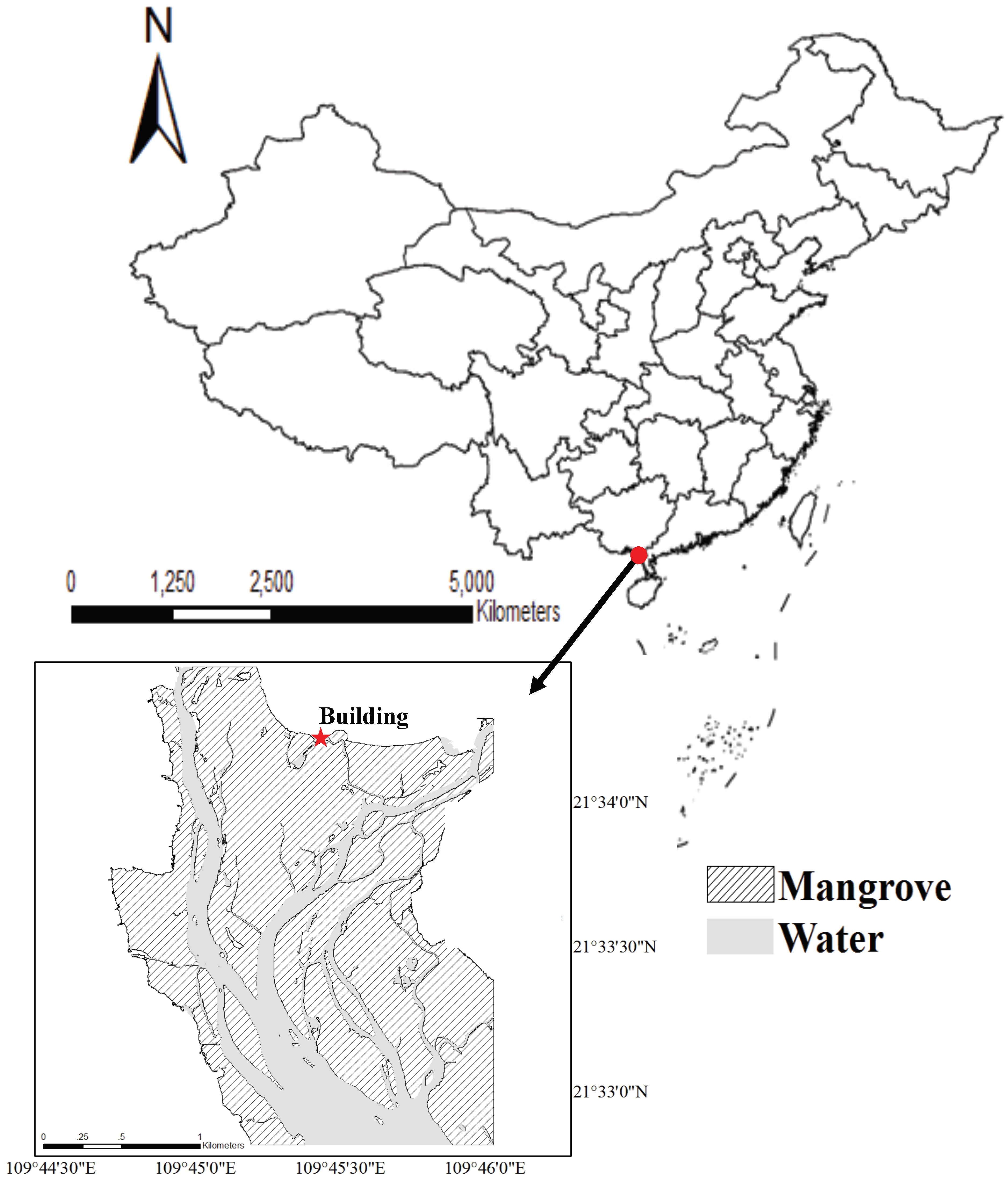
The Gaoqiao Mangrove Reserve [17,20] is located in southern China at the coastal margin of the border between Guangdong Province and the Guangxi Zhuang Autonomous Region (Figure 1). Fluctuations in water vapor transport associated with land–sea breezes and organized circulation and precipitation systems are strong. This mangrove forest is located in a subtropical monsoon region near the Tropic of Cancer, and is therefore subject to strong but intermittent convective activity during summer. The water cycle is heavily impacted by the rainfall and secondary circulations associated with these convective systems, along with large-scale water vapor transport, evaporation from nearby seas, and evapotranspiration within the mangrove area. Previous studies on atmospheric water cycling in mangrove ecosystems have focused mainly on local processes such as evapotranspiration [21,22]. Here, we supplement these studies by using measurements of isotopic composition in water vapor and precipitation collected at the Gaoqiao Mangrove Reserve during July 2017 together with meteorological data and Lagrangian back trajectories to explore the influences of large-scale transport and convective rainfall on the water budget of the atmospheric boundary layer above the mangrove forest. This study helps to constrain the role of large-scale atmospheric processes relative to local land–atmosphere exchange in the isotopic water budgets of mangrove forests at this and other nearby measurement sites.

2. Materials and Methods

2.1. Stable Water Isotopes

Heavy isotopes of water are rare in nature, accounting for less than 0.3% of water molecules [1]. Their ratios in water samples are therefore often expressed as deviations from a reference standard:

$$\delta =\frac{R}{R_{\mathrm{std}}}-1,$$

(1)

where R is the ratio of the heavy isotope to ${\mathrm{H}}_2{}^{16}\mathrm{O}$ in the sample and $R_{\mathrm{std}}$ is the equivalent ratio in the reference standard. In this study, isotopic ratios are expressed relative to Vienna standard mean ocean water (VSMOW), reported in per mille (%) for convenience. A positive value of $\delta$ indicates that the relative abundance of the rare isotope is enriched in the sample relative to VSMOW. Conversely, a negative value of $\delta$ indicates that the sample is depleted of the rare isotope relative to VSMOW. A value of $\delta =-1000$% would indicate that the sample is completely depleted of the rare isotope.

The fractionation of isotopes during phase changes is measured by the fractionation factor $\alpha$, where

$${\alpha }_v^l=\frac{R_l}{R_v}$$

(2)

represents the fractionation of isotopes during exchange between liquid (l) and vapor (v). Laboratory measurements and physical considerations provide strong constraints on the fractionation factor at thermodynamic equilibrium [23], which depends on the temperature at the liquid–vapor interface. Thermodynamic equilibrium fractionation between liquid and vapor presumes that an equal number of water molecules is exchanged in each direction. Effectively, this requires that vapor in a thin layer above the liquid water interface be saturated at the temperature of the interface. At our coastal mangrove site, important deviations from these conditions could include evaporation from an open water surface when relative humidity (RH) is small or winds are large, as well as the incomplete evaporation of falling raindrops into unsaturated air (RH < 1). Fractionation under these non-equilibrium conditions is referred to as kinetic fractionation, and can be estimated via empirically-based parameterizations.

Deuterium excess $\left(\mathrm{d-excess}\right)$, calculated via the formula

$$\mathrm{d-excess}=\delta \mathrm{D}-8·{\delta }^{18}\mathrm{O},$$

(3)

is insensitive to (reversible) equilibrium fractionation, and is therefore often used to infer the location or meteorological conditions that characterize the vapor source region under the assumptions that kinetic effects and water loss during transport are small [24,25]. Several recent studies have suggested that the interpretation of $\mathrm{d-excess}$ is less straightforward than originally thought [26,27,28,29]; however, as a general rule, values of d-excess are positively correlated with temperature and negatively correlated with RH at the evaporative source. These signals may be confounded by other factors, such as strong winds at the evaporative source or the partial evaporation of falling rain [24,30]. The latter sensitivity may also permit the use of d-excess in assessing the relative fraction of rain evaporation below clouds.

Several simple models are used to benchmark isotopic behavior [3,31]. In this work, we employ the Rayleigh distillation model and a model for mixing between two unsaturated air masses. The Rayleigh distillation model tracks the evolution of water isotopes within an air parcel assuming that the parcel does not mix with its environment and that any condensate that forms falls out of the air mass immediately as precipitation. The isotopic ratio of the residual water vapor in the air parcel, R, is then described by the formula

$$\mathrm{d}\ln R=(\alpha -1)\mathrm{dln}q,$$

(4)

where $\alpha$ is the temperature-dependent fractionation factor (assuming thermodynamic equilibrium) and q is the mass mixing ratio of water vapor. Mixing between two unsaturated air masses with different isotopic compositions is modeled by

$${\delta }_m=\frac{f{\delta }_0{q}_0+(1-f){\delta }_1{q}_1}{f{q}_0+(1-f)q_1},$$

(5)

where ($q_0$, ${\delta }_0$) and ($q_1$, ${\delta }_1$) represent the specific humidity and isotopic content of the two air masses and $f\in [0,1]$ is the fractional contribution of the first air mass ($m_0$) to the total mass ($m_0+m_1$) after mixing [31]. The resulting values ${\delta }_m$ represent the isotopic content of the mixture.

2.2. Description of Site Measurements

Gaoqiao Mangrove Reserve is located at the northwest corner of Leizhou Peninsula, adjacent to the South China Sea and centered at ${21}^{\circ }{33}^{\prime }$ N, ${109}^{\circ }{45}^{\prime }$ E (Figure 1). The average summertime temperature is $29.5{}^{\circ }$C, ranging as high as $38.1{}^{\circ }$C. Precipitation occurs mainly during the summer and autumn, often in the form of strong convection and thunderstorms. Conditions over the nearby sea are likewise characterized by high temperature and high humidity. During the rainy season, air in the middle and lower troposphere above the mangrove is affected by the southwest monsoon. Organized precipitation may arise from a range of factors, including tropical cyclones, mesoscale convective systems and fronts.

The observatory is located at ${21}^{\circ }{34}^{\prime }{12}^{″}$(21.57) N, ${109}^{\circ }{45}^{\prime }{25}^{″}$(109.76) E. The building is more than 10 m high and located only about 10 m away from the edge of the mangrove forest. Measurements of the isotopic composition of water vapor were collected using a Picarro L2130-i cavity ring-down laser spectrometer (CRDS), with single-measurement precisions (1$\sigma$) of 0.12% for ${\delta }^{18}$O and 0.3% for $\delta$D. The instrument was housed inside the observation station, with the inlet fixed near the top of the building approximately 10 m above ground level. During the campaign, a suction pump continuously imported air through Teflon tubing 20 m in length. The inlet was protected by a multi-layer plastic cover to prevent raindrops from entering the tubing. The instrument was monitored continuously from 7:00 to 19:00 local time during 11–28 July, and was controlled remotely through a wireless network at other times during the study period. The instrument was connected to an uninterruptible power supply (UPS) capable of providing temporary auxiliary power when needed; however, an extended power outage starting in the early morning on 17 July local time resulted in a data gap of nearly one day. No other instrument stoppages occurred during the study period.

Although meteorological measurements are often collected at a flux tower about 300 m from the observatory, most of the measurements collected at this tower during our measurement period were corrupt and unusable. We substitute these with meteorological data collected at a separate flux tower located about 3 km away from the observatory site. Measurements collected at this tower include air temperature, soil temperature, relative humidity, rainfall rate, wind speed and wind direction, all at a sampling frequency of 30 min. The similar altitude (sea level) and proximity of this tower to the observatory support the use of these data to represent local meteorological conditions during this study.

Rainwater samples were collected using a rain gauge placed on the roof of the building that also housed the CRDS instrument. At the end of each rainfall event, rainwater was transferred from the measuring cylinder into a clean sample bottle after rinsing the bottle three times with rainwater to eliminate residue. Once filled, each sample bottle was wrapped several times with parafilm to prevent water leakage, evaporation, or isotopic exchange. The sample bottles were then stored in a refrigerator with an internal temperature of 4${}^{\circ }$C. At the end of the study period, all water samples were placed in an insulated container and transported to the laboratory for isotopic analysis. The isotopic compositions of rain samples were measured using a Thermo Scientific MAT 253 isotope ratio mass spectrometer equipped with a Flash 2000 HT elemental analyzer. The measurement accuracy is within ±1% for $\delta \mathrm{D}$ and ±0.2% for ${\delta }^{18}\mathrm{O}$. Of the 33 rainfall events that occurred during the observation period, 22 were successfully sampled for inclusion in this analysis.

2.3. Calibration

The isotopic content of water vapor measured by a CRDS instrument must be calibrated, as described by previous studies [32]. Two standard waters were used for calibration during the observation period. The isotopic compositions of both standards were measured in the laboratory using the same isotope ratio mass spectrometer used to process the rain samples. The average isotopic ratios obtained were $\delta \mathrm{D}=-154.31$% and ${\delta }^{18}\mathrm{O}=-20.69$% for standard 1 and $\delta \mathrm{D}=-49.81$% and ${\delta }^{18}\mathrm{O}=-7.07$% for standard 2.

A calibration check was performed after every 6 hours of instrument operation using a Picarro A0101 Standards Delivery Module (SDM) and a Picarro A0211 high-precision vaporizer in the manufacturer-recommended setup. Based on all calibration steps conducted during the campaign, we derive the correction equations for $\delta \mathrm{D}$ and ${\delta }^{18}\mathrm{O}$ as

$$\delta {\mathrm{D}}_{\mathrm{cal}}=1.1624\delta {\mathrm{D}}_{\mathrm{raw}}+6.0899$$

(6)

$${\delta }^{18}{\mathrm{O}}_{\mathrm{cal}}=1.2243{\delta }^{18}{\mathrm{O}}_{\mathrm{raw}}+0.1235$$

(7)

where $\delta {\mathrm{X}}_{\mathrm{raw}}$ represents the measured value before calibration and $\delta {\mathrm{X}}_{\mathrm{cal}}$ represents the value after calibration. No systematic shifts or drifts occurred during the observation period. Although the calibration considers humidity-dependent biases, the consistently high humidities at this site during the measurement period mean that this dependence is unlikely to have any meaningful impact on our isotopic measurements. Humidity-dependent effects are therefore not considered here. In addition, data collected during the 5 min after each calibration step were discarded to reduce the potential influence of residual vaporized standard water on our measurements of water vapor in ambient air. For ease of presentation and comparison with other variables, all data are averaged in 30-min windows (i.e., 48 time windows per day). Depending on the timing of calibration steps and other instrument outages (see above), data may be missing or incomplete in some time windows. Such differences in coverage are accounted for in the uncertainty calculations. All data are presented in local solar time (UTC+8) unless otherwise specified.

Systematic biases have been reported in humidity measurements collected using Picarro CRDS instruments. In related studies, these measurements have been calibrated against humidity values measured by a companion instrument or instruments [5]. Based on three days of coincident measurements collected by a LI-6400 instrument and the Picarro CRDS in series during December 2015 [20], we adjust the humidity values according to the equation

$$q_{\mathrm{cal}}=1.04q_{\mathrm{raw}}+2.81,$$

(8)

where $q_{\mathrm{raw}}$ represents the measured value prior to calibration and $q_{\mathrm{cal}}$ represents the calibrated value. Both variables are expressed as water vapor volume mixing ratios.

2.4. Trajectory Calculations

Lagrangian trajectories are calculated using the open-source FLEXPART (FLEXible PARTicle) model [33], which has been widely used in studies of atmospheric transport [34,35,36,37]. We use the FLEXPART model in its backward configuration, in which the Lagrangian trajectories of a large number of particles are computed backward in time according to the large-scale wind field and parameterized sub-gridscale processes [33]. Sub-gridscale processes considered by FLEXPART include moist convection and boundary layer turbulence. Both parameterizations are enabled in our calculations. The FLEXPART simulations used in this paper are driven using six-hourly analyses and 3-hourly forecast fields from the European Centre for Medium-Range Weather Forecasts (ECMWF) Interim Reanalysis (ERA-Interim) [38]. All reanalysis products are provided on a $1^{\circ }\times 1^{\circ }$ latitude–longitude grid with 60 hybrid $\sigma$-p vertical levels extending from the surface to 0.1 hPa.

The area studied is a small cell ${0.1}^{\circ }$ (∼10 km) on each side centered at the observatory site (${21.57}^{\circ }$ N, ${109.76}^{\circ }$ E). Trajectories are calculated to track the moisture sources for water vapor in the atmospheric surface layer. The air from 15 m above ground level (AGL) to 50 m AGL is evenly divided into 1000 particles by volume. Trajectories are released once every 3 h and integrated backward in time for 5 days. Over the 30-day duration of the observational campaign in July 2017, this results in $8\times 30=240$ sets of 1000 trajectories, for a total of 240,000 trajectories. The vertical range from 15 m to 50 m AGL is selected to represent the turbulent surface layer above the canopy, and to approximately match the intake height of the water vapor isotopic analyzer. The integration length is set at 5 days to balance parcel “integrity” (i.e., to reduce the effects of unrepresented mixing during transport) against the objective of reliably identifying the geographical distribution of moisture sources (see following section). Releases every three hours allow us to characterize any diurnal cycle or day-to-day variations in dominant moisture sources and transport pathways. Coordinate information (including longitude, latitude, and AGL height) and physical information (including specific humidity and temperature) are stored at every output time step.

2.5. Moisture Source Attribution

We identify and quantify moisture source contributions following the method proposed by Sodemann et al. [37] and recently adapted by Huang et al. [39]. For an air parcel of constant mass m traversing a column of atmosphere, we assume that any increase in the water vapor mass mixing ratio occurs via the mixing of local evaporation into the parcel, while any decrease in water vapor occurs via the formation and loss of precipitation from the parcel. Changes in the water vapor content of the parcel (q) as it passes through the column are used to infer the net balance of moisture gains and losses by the parcel ($e-p$) within that area:

$$e-p=m\frac{dq}{dt}.$$

(9)

Assessing the cumulative gains and losses of all N air parcels that pass through the atmospheric column above a given area, we arrive at the formula

$$E-P\approx {\displaystyle \sum _{i=1}^N}(e-p)\approx {\displaystyle \sum _{i=1}^N}m\frac{dq}{dt},$$

(10)

where E represents the evaporation per unit time over the area, P represents the amount of rainfall per unit time in the area, and $E-P$ represents the net evaporation or rainfall (i.e., the water flux). When $E-P>0$, this implies a net gain of moisture by parcels that pass through the area on their way to the target domain. When $E-P<0$, this conversely implies a net loss of moisture by parcels that pass through the area on their way to the target domain. This simplification reflects the observation that either evaporation or rainfall dominates the local moisture flux evaluated over short periods [40]. Areas where net evaporation is identified are considered as sources of water vapor.

The output of the FLEXPART model is used to calculate specific humidity differences between adjacent output time steps along each track. These differences are taken to represent the changes of water vapor content in the corresponding air parcels during this period. Please note that this calculation proceeds forward in time (q at the later time is subtracted from q at the earlier time), as opposed to the trajectories, which are integrated backward in time. Given these differences, Equation (10) is applied to estimate the net gain or loss of moisture over each location in the grid.

A positive value of $E-P$ over a particular area does not necessarily mean that the entirety of the moisture gain is transported from the source location to the target domain. Specifically, if rainfall occurs later along the trajectory ($E-P<0$), the contributions of all previous moisture gains are assumed to decrease proportionately. Such increases and decreases of water vapor content may occur many times along the trajectory. The moisture sources for surface layer water vapor at 3-hourly intervals and for tropospheric moisture during rain events are calculated by applying this algorithm to the two families of trajectories described in Section 2.4.

3. Local Conditions

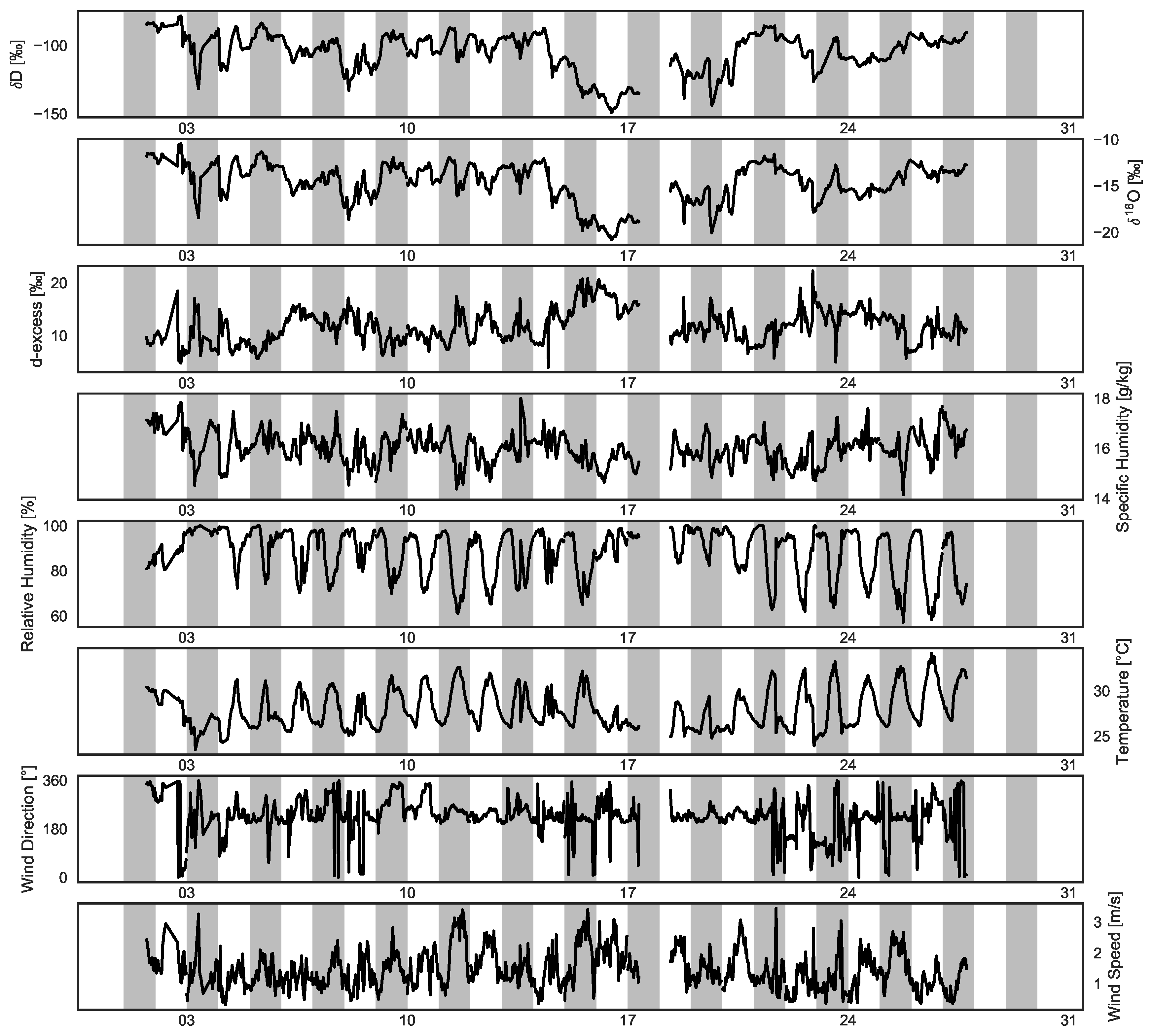
Figure 2 shows the measurements collected by the water vapor isotopic analyzer and at the nearby weather station during the observation period. All data are shown at 30-min intervals from 17:30 LST 1 July 2017 through 18:00 LST 27 July 2017. Summary statistics of these core variables ($\delta \mathrm{D}$, ${\delta }^{18}\mathrm{O}$, d-excess, surface air temperature, specific humidity, relative humidity, and wind speed) are listed in

Table 1. Water vapor isotopic composition and atmospheric conditions observed at Gaoqiao Mangrove Reserve during July 2017.

	Whole Period		During Rainfall
	Mean	Standard Deviation	Mean	Standard Deviation
$\delta \mathrm{D}$ (%)	−105.27	14.22	−150.66	19.61
$\delta {}^{18}\mathrm{O}$ (%)	−14.62	2.08	−21.19	2.64
d-excess (%)	11.73	3.06	18.84	3.38
T (${}^{\circ }$C)	27.99	2.14	27.05	2.03
q (g/kg)	16.01	0.62	15.65	0.46
RH (%)	87.86	10.53	90.78	9.30
WS (m/s)	1.45	0.61	1.93	0.47

. Data within three standard deviations of the mean (approximately 99.7% of the data) are selected for further analysis. Near-surface winds at the site typically range southwesterly to southeasterly (∼80% of measurements at 10-min sampling resolution), with speeds only rarely exceeding 4 m s${}^{-1}$. The prevailing winds are therefore directed across the forest toward the measurement site (Figure 1), indicating that our measurements can well represent the isotopic content of water vapor in the atmospheric surface layer above the mangrove forest.

Among the variables included in Figure 2 and Table 1, only surface air temperature, relative humidity, and wind speed had clear diurnal cycles during the observational period. The mean diurnal cycle in surface air temperature consists of an extended minimum of ∼26–27${}^{\circ }$C during the early morning hours, followed by a sharp rise between 8:00 and noon local time. Surface air temperature peaked at ∼31${}^{\circ }$C at 15:00 before beginning its gradual relaxation back to the nighttime minimum. The mean diurnal cycle in relative humidity is qualitatively opposite to that in temperature, with a maximum of more than 95% in the morning around 7:00 and a minimum of less than 75% in the afternoon around 15:00. The mean diurnal cycle in wind speed consists of a step change from ∼1.0 m s${}^{-1}$ during the early morning hours to ∼1.8 m s${}^{-1}$ between 10:00 and 20:00. The morning increase in wind speed, which occurs between 8:00 and 10:00, is more abrupt than the evening decline, which occurs between 20:00 and midnight.

No significant diurnal cycle was observed in the isotopic composition of water vapor, although the ${\delta }^{18}$O, $\delta$D, and d-excess ratios are all slightly larger between 10:00 and 15:00, broadly consistent with the diurnal peak in the ratio of transpiration to evapotranspiration within the Zhangjiang Mangrove Reserve (Liang et al., submitted manuscript). Both ${\delta }^{18}$O and $\delta$D are significantly correlated with temperature ($r=0.55$) and anti-correlated with relative humidity ($r=-0.51$). However, despite a weak qualitative consistency in the diurnal cycle, these statistical relationships between isotopic ratios and meteorological data emerge almost entirely from day-to-day co-variability (Figure 2).

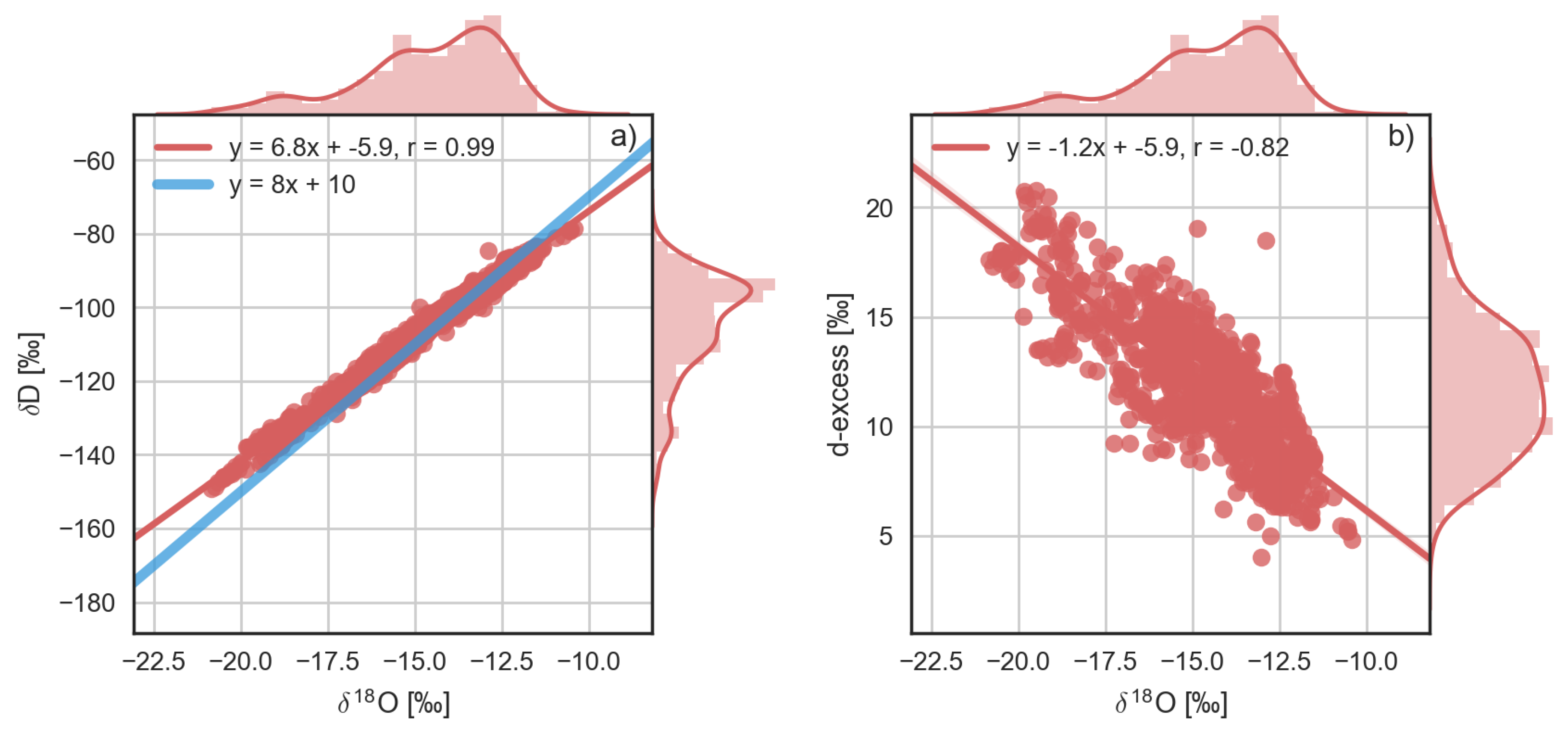
Figure 3 summarizes variations in the isotopic composition of water vapor during the study period. The linear relationship between ${\delta }^{18}\mathrm{O}$ and $\delta \mathrm{D}$ is well-known, with vapor measurements often also following the global meteoric water line (GMWL; $\delta \mathrm{D}=8\times {\delta }^{18}\mathrm{O}+10\%$) first identified in measurements of isotopic ratios in precipitation [3]. Our measurements of isotopes in water vapor (Figure 3a) trace a local atmospheric water line with a slightly shallower slope (6.8) and a smaller intercept ($-5.9$%) relative to the GMWL. Potential contributors to these differences include wind speeds during evaporation from the nearby sea surface, isotopic distillation during transport, partial evaporation of raindrops during rainfall, and the ratio of transpiration to evaporation in the local ecosystem, among others [26,27,28,29,30]. Figure 3b further shows that the value of d-excess is inversely related with ${\delta }^{18}$O. Although global model simulations suggest that smaller (more negative) d-excess and larger (more positive) ${\delta }^{18}$O over land areas can often be attributed to a relatively strong influence of transpiration [41], it is unclear whether this expectation holds for mangrove ecosystems. Additional measurements of isotopic ratios in water vapor at the Gaoqiao site indicate that the smallest d-excess values are associated with ambient conditions below the mangrove canopy, with considerably larger values of d-excess observed in direct measurements of transpiration at the leaf interface (J. Liang, unpublished data). Larger (more positive) d-excess and smaller (more negative) ${\delta }^{18}$O could also be associated with evaporation into relatively dry air over nearby ocean sources or Rayleigh-type distillation during large-scale transport [1].

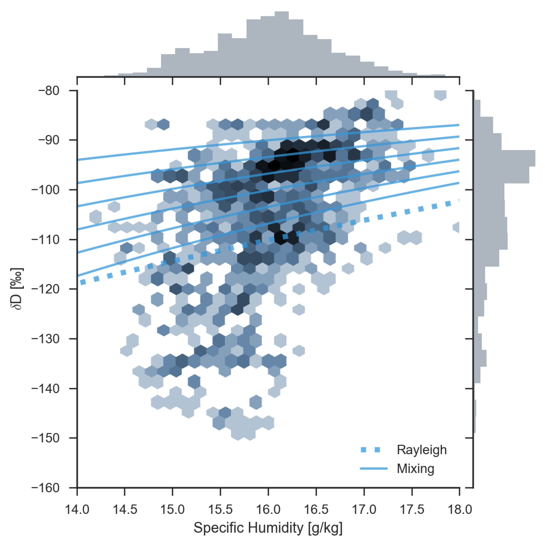
Figure 4 shows the joint distribution of observations of $\delta$D and specific humidity (q) collected at the measurement site. Selected theoretical model results are also shown for context. The bulk of the distribution can be explained by air-mass mixing (Equation (5)) between humid boundary layer air that is relatively enriched in heavy isotopes and drier free tropospheric air that is relatively depleted in heavy isotopes. The definitions of both end members are guided by typical outputs for July from a global model nudged toward reanalysis products [42]. The humid end member is assumed to have 95% relative humidity at 30${}^{\circ }$C and $\delta$D = $-80$%, roughly characteristic of calm conditions over the nearby South China Sea. A range of dry end members are defined with $q=9.3$ g kg${}^{-1}$ and values of $\delta$D that span the range of free tropospheric values simulated by the model near the Gaoqiao site. With this definition of the dry end members and over this range of specific humidities, the Rayleigh distillation curve is nearly parallel to the lower range of the mixing lines. A substantial fraction of the observations are located in the super-Rayleigh portion of the $q-\delta$D phase space [29,31], again suggesting that rain re-evaporation (local or upstream) plays an important role in setting the isotopic composition of surface-layer water vapor at the measurement site.

4. Local Rain–Vapor Exchange

Details of rainfall events during the observation period are listed in

Table 2. Details of rain events during the observation period. Blank cells indicate that the corresponding data were not collected.

Event	Start Time	Stop Time	$\mathit{\delta }\mathbf{D}$ (%)	$\mathit{\delta }{}^{18}\mathbf{O}$ (%)	d-Excess (%)	Rainrate (mm h${}^{-1}$)
1	7/13 13:49	7/13 14:30	−87.17	−14.56	29.31
2	7/14 11:11	7/14 11:41
3	7/14 14:15	7/14 14:28	−76.47	−13.83	34.17	138.9
4	7/15 13:35	7/15 13:45	−86.69	−13.42	20.67
5	7/16 07:00	7/16 07:20
6	7/16 07:45	7/16 08:00
7	7/16 08:18	7/16 10:15	−94.13	−14.98	25.71	6.7
8	7/16 11:03	7/16 11:53	−100.77	−15.35	22.03	8.5
9	7/16 12:19	7/16 12:43
10	7/16 15:57	7/16 16:14				13.8
11	7/16 16:23	7/16 16:32
12	7/16 16:46	7/16 16:53
13	7/16 16:57	7/16 17:30	−85.94	−13.69	23.58	5.6
14	7/16 17:44	7/16 18:00
15	7/16 18:18	7/16 18:33	−82.03	−13.46	25.65	48.4
16	7/16 18:48	7/16 19:25	−78.23	−12.68	23.21	6.2
17	7/17 07:00	7/17 07:30
18	7/17 14:20	7/17 14:32	−53.87	−11.07	34.69	98
19	7/17 14:57	7/17 15:03	−48.74	−9.2	24.86	100
20	7/17 15:14	7/17 15:17
21	7/18 04:00	7/18 07:00	−43.17	−8.9	28.03	14.9
22	7/18 08:26	7/18 10:46	−43.34	−9.44	32.18	3.5
23	7/18 10:59	7/18 11:32
24	7/18 18:30	7/18 22:30	−49.23	−10.1	31.57	32
25	7/19 08:49	7/19 09:52	−58.27	−9.45	17.33	1.0
26	7/19 14:29	7/19 14:57	−71.96	−11.64	21.16	117.4
27	7/19 15:27	7/19 17:50	−96.78	−15.11	24.1	7.1
28	7/21 16:29	7/21 17:20	−33.94	−7.68	27.5
29	7/22 21:30	7/22 22:30	−80.55	−13.47	27.21	38.6
30	7/23 16:41	7/23 17:10	−44.54	−9.77	33.62	64.1
31	7/23 17:58	7/23 18:32	−42.73	−9.84	35.99	84.4
32	7/24 13:19	7/24 13:29	−58.14	−10.52	26.02	20.4
33	7/28 13:25	7/28 13:42	−42.6	−9.12	30.36	47.3

. Conditions were systematically cooler and more humid during rain events, with larger wind speeds and wind directions mainly from the southwest. Most of the rainfall events occurred around middle to late afternoon, between 14:00 and 19:00. These afternoon rain events were frequently accompanied by thunderstorms, consistent with the gradual destabilization of the atmosphere to convection as temperature approaches its mid-afternoon maximum. In addition, many of the rainfall events lasted for less than 30 min. The intermittent nature and short durations of these events suggest that they represent spontaneous local convection that is not well-organized at larger scales.

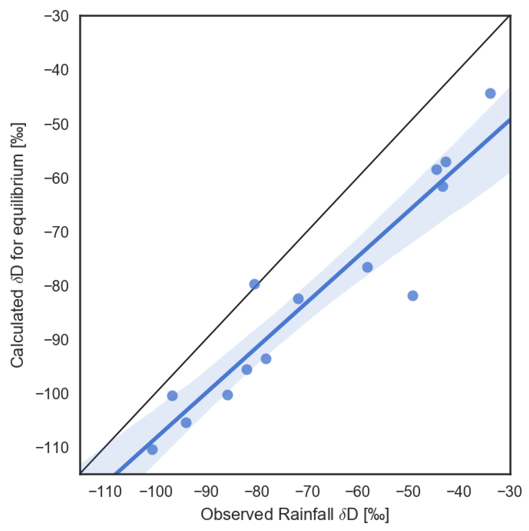
The linear correlation coefficient (r) between ${\delta }^{18}\mathrm{O}$ in rainfall and ${\delta }^{18}\mathrm{O}$ in vapor is 0.80 ($p<0.01$). This large correlation may be due to surface water vapor entering the convective system through updrafts [43], or isotopic equilibration of water vapor with raindrops falling through the boundary layer [44]. Figure 5 shows a comparison between observed values of $\delta \mathrm{D}$ in rainfall and theoretical values based on equilibration with the observed isotopic composition of water vapor at a temperature of 27${}^{\circ }$C (the average temperature associated with rainfall events during the observation period; Table 1). Although the expected and observed values are strongly correlated, the expected values are typically more depleted of heavy isotopes than the observed values. This difference indicates that equilibration between boundary layer vapor and rainfall was incomplete, and further suggests that non-equilibrium isotopic fractionation may have taken place through partial evaporation of the raindrops produced by these storms. This possibility can be further explored by calculating the ratio $R_p/R_v$, which would equal the equilibrium fractionation factor if the measured rainfall and the measured vapor were in isotopic equilibrium. Deviations from the equilibrium fractionation factor, particularly toward larger values, may thus indicate kinetic isotopic exchange associated with rain re-evaporation [8].

The maximum and minimum values of $R_p/R_v$ for HDO during the measured rainfall events are 1.117 and 1.073, with a mean value of $1.092\pm 0.009$. Considering only the influence of temperature on fractionation at thermodynamic equilibrium, the mean measured value of $R_p/R_v$ corresponds to a temperature of approximately 14${}^{\circ }$C. This temperature is much colder than the typical temperature during rainfall events (27${}^{\circ }$C), indicating the influences of other processes besides isotopic equilibration. Such processes include rain re-evaporation or water vapor mixing into the boundary layer from the cloud layer [12,45]. The effective fractionation associated with partial evaporation of raindrops into unsaturated air can be expressed as [46]:

$${\alpha }_{\mathrm{eff}}=\frac{{\alpha }_{\mathrm{eq}}·\mathrm{RH}}{1+(\mathrm{RH}-1)·{\alpha }_{\mathrm{eq}}·{\mathrm{df}}^{0.58}}$$

(11)

where ${\alpha }_{\mathrm{eq}}$ is the equilibrium fractionation factor, RH is the relative humidity, and $\mathrm{df}=1.025$ is the ratio of the molecular diffusivity of ${\mathrm{H}}_2{}^{16}\mathrm{O}$ to that of HD${}^{16}$O [24]. The exponent 0.58 is set to correspond to re-evaporation of rain droplets approximately 1 mm in size [47]. As relative humidity decreases, $R_p/R_v$ increases, reflecting stronger non-equilibrium fractionation. The average measured value of $R_p/R_v$ (1.092) is achieved with a temperature of 27${}^{\circ }$C and a relative humidity of 87%, consistent with average values of temperature (27${}^{\circ }$C) and relative humidity (90%) during the measured rainfall events (Table 1). The maximum value of $R_p/R_v$ (1.117) could result if RH decreased to 72% while maintaining a temperature of 27${}^{\circ }$C, while the minimum value (1.073) suggests equilibration between vapor and rainfall (RH = 100%) at a warmer temperature of 31${}^{\circ }$C. Please note that this framework provides a plausible but not unique interpretation of isotopic disequilibrium between rain and vapor. For example, the base assumption of rain–vapor equilibrium does not hold if the time scale of isotopic equilibration is long relative to the time the raindrop spends transiting the well-mixed layer [44]. In this case, some portion of the disequilibrium would arise from differences between isotopic ratios in surface-layer vapor (as reflected in fully equilibrated rain) and isotopic ratios in the vapor from which the rain formed (as reflected in the isotopic composition of rainfall at cloud base).

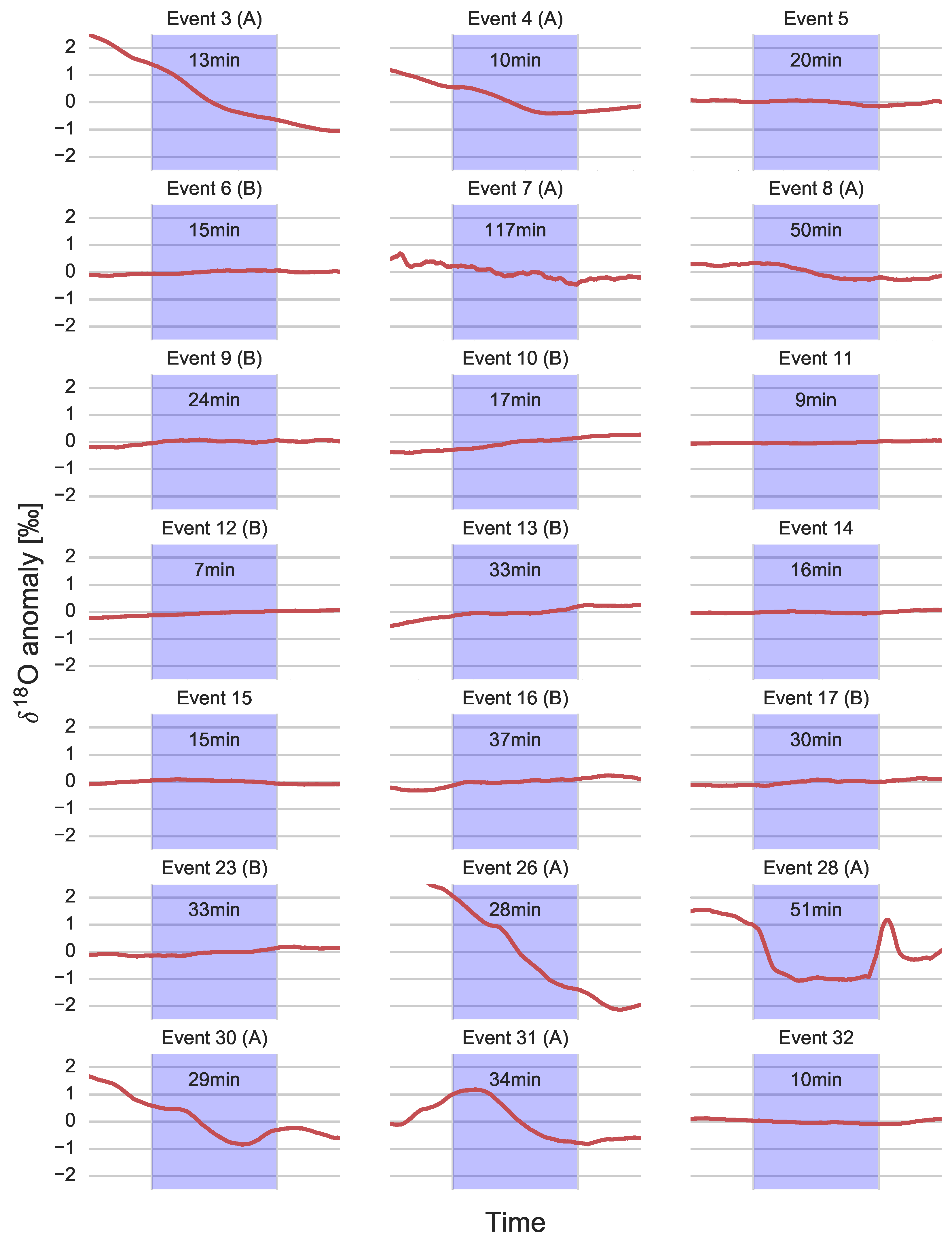
To support a more detailed exploration of the rainfall events, Figure 6 shows changes in ${\delta }^{18}$O during each rainfall event. Please note that water vapor isotopic composition was not successfully measured during all rainfall events, with gaps arising both from the extended power outage mentioned above and scheduled calibration steps for the CRDS instrument. Events with measurement gaps are omitted from Figure 6, leaving 21 rainfall events with full coverage. In addition to measurements collected during rainfall events, data are also plotted for the periods immediately preceding and following each rainfall, with each added segment spanning 50% of the duration of that event. For example, if the duration of a rainfall event is 40 min, data are also shown for 20 min before the start of the event and 20 min after the conclusion of the event, so that the total time shown is twice the duration of the rainfall. The duration of each rainfall event is noted in the corresponding panel of Figure 6. The Picarro CRDS analyzer has a measurement frequency of ∼1 s. To reduce the effects of noise, data collected during each event are processed using a ∼5-min sliding average. We use the ‘boxcar’ window function, meaning that all points within the window are equally weighted. Examining Figure 6 in the context of the information provided in Table 2 shows that this procedure is effective at reducing the ‘noise’ (small-scale fluctuations) in isotopic vapor measurements during individual events.

The evolution of ${\delta }^{18}$O clearly differs among different rainfall events. We begin by naively classifying rainfall events into two main types based on changes in isotopic composition. The first type, which we refer to as class ‘A’, exhibits an evident decrease (of at least 0.5%) in ${\delta }^{18}$O over the duration of the event. Eight rain events are assigned to class A, including event 3, event 4, event 7, event 8, event 26, event 28, event 30, and event 31. The second type contrasts with the first, in that it exhibits at least a slight increase in ${\delta }^{18}\mathrm{O}$ (of at least 0.1%) over the lifetime of the event. This threshold exceeds the uncertainty threshold under the 5-min rolling average, and is chosen to ensure the same number of events in each class. We refer to the second (neutral–increasing ${\delta }^{18}\mathrm{O}$) type as class ‘B’, which also contains eight rain events: event 6, event 9, event 10, event 12, event 13, event 16, event 17, and event 23. The evolutions of ${\delta }^{18}$O during five rainfall events (event 5, event 11, event 14, event 15 and event 32) do not match the criteria for either type A or type B and are omitted from the comparison. Changes in the isotopic composition of water vapor experienced during a rain event typically persist after the end of the event, although the extent of this persistence varies.

Exchange of heavy isotopes between falling raindrops and environmental water vapor may reduce the fractions of heavy isotopes in water vapor and increase the fractions of heavy isotopes in rainfall, particularly when a substantial portion of the raindrops have formed from isotopically depleted vapor at low temperatures in the upper levels of strong convection. Intense downdrafts of dry air with low ratios of heavy isotopes may also act to reduce the content of heavy isotopes in boundary layer water vapor during the passage of strong convective systems [45]. Decreases in ${\delta }^{18}$O associated with type A rainfall events were relatively intense, and were usually accompanied by sharp drops in locally measured values of temperature and specific humidity. These changes likely suggest a strong influence of downdrafts [45], vigorous rain–vapor exchange at relatively low values of RH [46], or an increasing influence of raindrops formed deeper in the atmosphere, where water vapor is more depleted of heavy isotopes [48]. By contrast, type B rainfall events typically showed increases in both vapor ${\delta }^{18}$O and specific humidity over the duration of the rainfall, suggesting limited downdraft activity, weaker kinetic exchange, and/or shallower cloud systems.

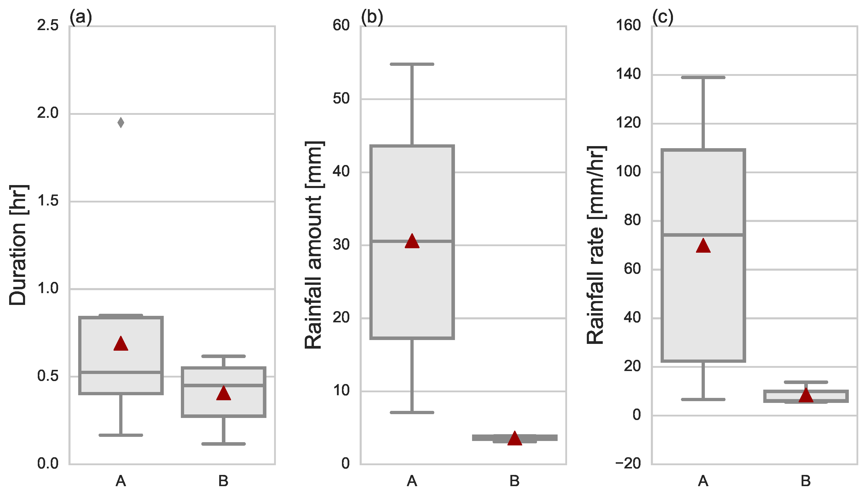
Figure 7 shows distributions of the duration, cumulative rainfall amount, and rainfall rate for type A and type B rainfall events. The average duration of type A events during our observation periods was longer than that of type B events. Differences in cumulative rainfall amount and rainfall rate were more profound, with both quantities almost uniformly larger during type A events than during type B events. Connecting these observations to the more extensive measurements collected by Tremoy et al. [7] in Niamey, Nigeria, we suggest that type A rainfall events correspond to large-scale, organized deep convective systems (their type A). The relatively low rainfall rates and evolution of ${\delta }^{18}$O associated with our type B rainfall events are more consistent with their type C, considered to be primarily isolated convective events of a more local origin.

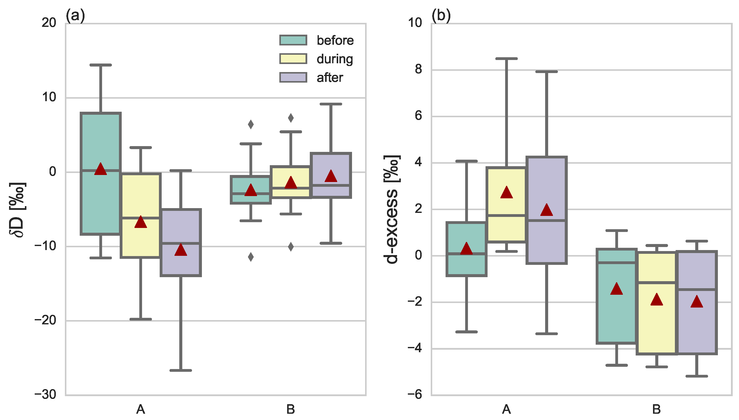
To further test this hypothesis, we calculate changes in $\delta$D and d-excess in boundary layer water vapor before, during, and after the type A and type B rainfall events, respectively, using the same definitions of these periods as in the construction of Figure 6. The results are shown in Figure 8 as anomalies relative to the daily mean for the day when the rainfall event occurred, which reduces spread due to day-to-day variations that may be unrelated to the direct impacts of the rainfall event. As with ${\delta }^{18}$O, type A events were associated with a progressive reduction in $\delta \mathrm{D}$, while type B events were associated with a slight increase in $\delta$D. Type A events also showed an increase in d-excess of approximately 1∼2%, which tended to be most pronounced during the event. Indeed, all but one of the vapor measurements during type A rainfall events had d-excess values greater than the daily mean, an enhancement that often persisted after the rain stopped. By contrast, values of d-excess associated with type B events were typically smaller than the daily average. Despite only a slight change in the mean value of d-excess, the median value dropped by approximately 2∼3% over the course of the type B events. Perturbations in the isotopic composition of boundary layer water vapor during type A rainfall events typically exceeded those during type B events, with opposing behaviors in both first-order effects (i.e., ${\delta }^{18}$O and $\delta$D) and second-order effects (i.e., d-excess). These different behaviors are consistent with the hypothesized differences in convective organization between type A and type B events [7], as well as related differences in raindrop size [44], downdraft intensity [45], and vertical depth of convection [48]. Although this “amount effect” reasoning provides a set of working hypotheses for the differences between type A and type B events, the relative roles of these processes remain unclear, as do the conditions under which the dominant process may vary across rainfall systems or among locations. Longer time series sampling a larger number of rainfall events and additional observational context will be needed to further clarify these effects.

5. Large-Scale Transport

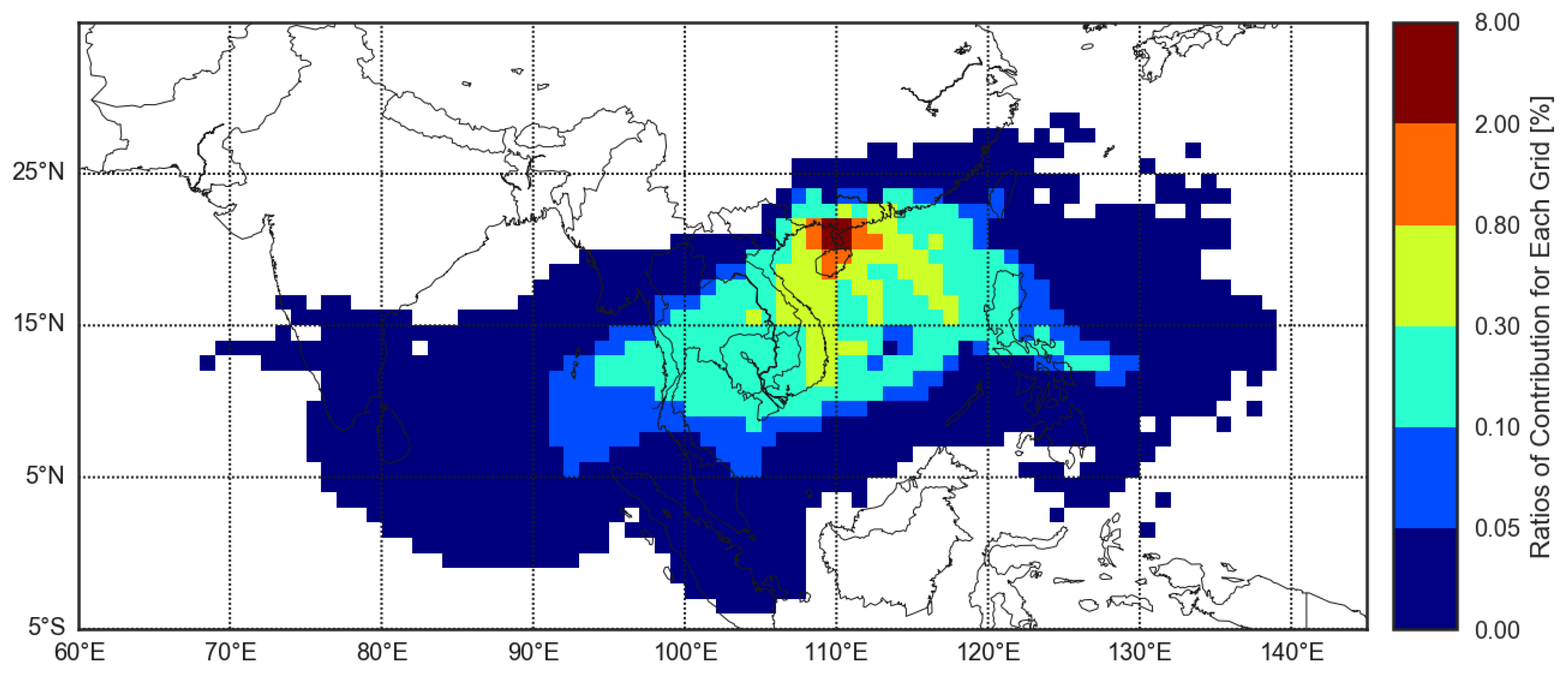
Figure 9 shows the horizontal distribution of the average attributed moisture source locations for surface-layer water vapor during the measurement campaign. The procedure for moisture source attribution is described in Section 2.5. Unshaded areas indicate areas that did not provide any moisture within the trajectory integration timescale. As a general rule, regions located farther from the site contributed smaller amounts of water vapor. Major source regions for surface-layer water vapor at Gaoqiao Mangrove Reserve include the Bay of Bengal, mainland Southeast Asia, the South China Sea, and land areas near the site (including Hainan Island and the Leizhou Peninsula).

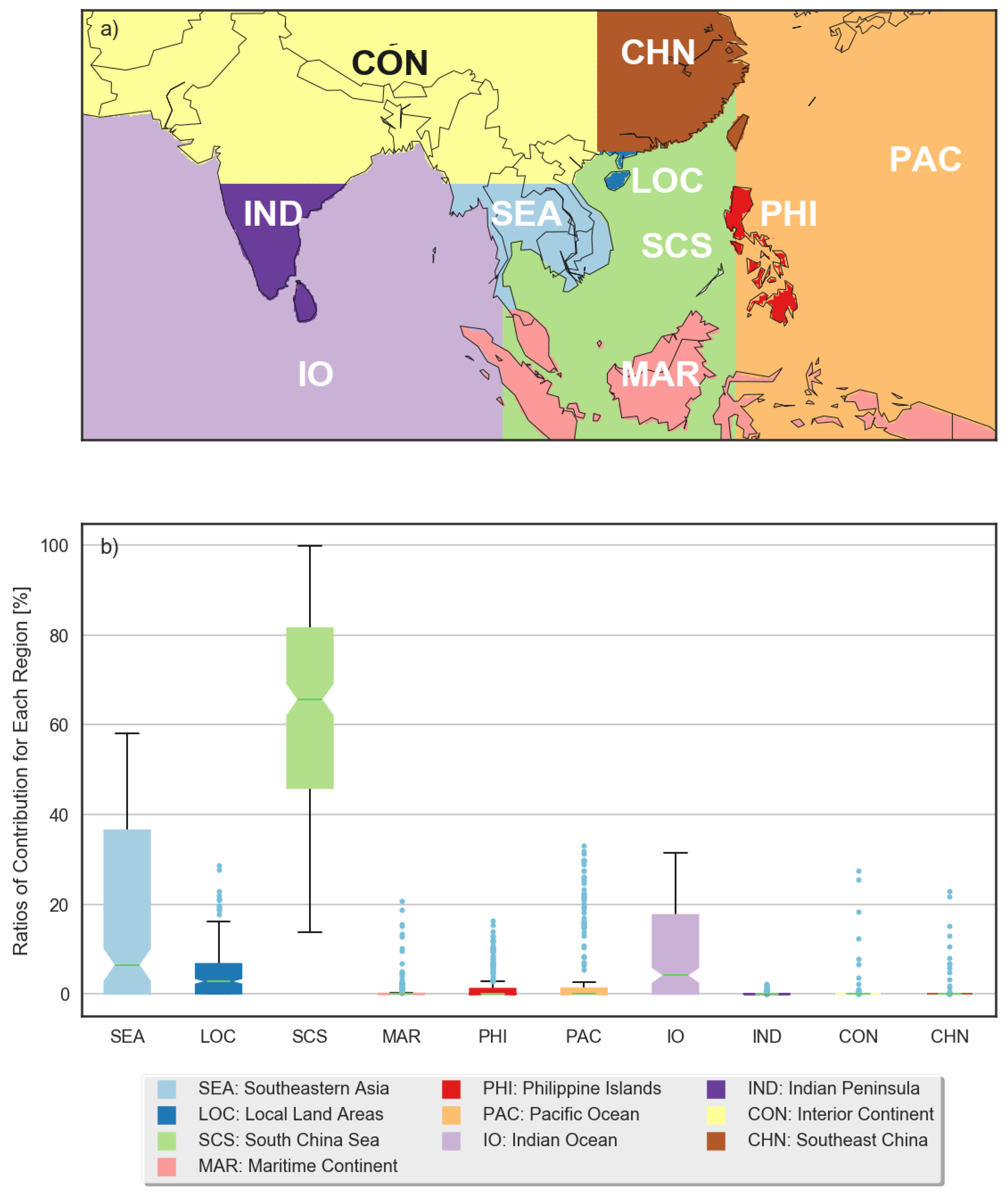
Figure 10a divides the regional domain into ten geographical sub-domains, including mainland Southeast Asia (SEA), the local land areas (LOC), the South China Sea (SCS), the Maritime Continent (MAR), the Philippine Islands (PHI), the Pacific Ocean (PAC), the Indian Ocean (IO), the Indian peninsula (IND), the Asian continental interior (CON), and southeastern China (CHN). The 240 separate source distributions calculated for Gaoqiao every three hours during July are then apportioned among these geographical sub-domains.

Figure 10b shows distributions summarizing the ranges of relative moisture contributions from each region. Here, relative moisture contributions from a specific region are defined as the ratio of the moisture contribution from that region to the total identified moisture source. The SCS, SEA, IO, and LOC domains are the major sources of moisture to the boundary layer above the Gaoqiao mangrove. Land regions contribute approximately 25% of the moisture. Oceanic regions contribute the remaining 75%, highlighting the dominance of oceanic sources. This partitioning between land and ocean sources is in good agreement with the results of van der Ent et al. [49], who estimated that continental recycling contributes about 20–30% of the moisture for precipitation in this region both year-round and in July.

The average contribution from the SCS domain is 63%, owing to its proximity to the Gaoqiao mangrove and the prevalence of southerly-to-southwesterly near-surface winds during the measurement campaign (Figure 2). The mean contribution of the SEA domain is also relatively large at approximately 16%, consistent with the importance of the southwest monsoon circulation in this region. Local land areas contribute approximately 5% of the moisture. This term may be approximately regarded as ‘local moisture recycling’; however, we caution that the small target domain at Gaoqiao (∼10 km$\times$10 km$\times$50 m) and the relatively coarse resolution of the reanalysis products used to drive the trajectory model render this estimate unreliable. The Indian and Pacific Ocean domains respectively accounted for around 9% and 4% of the total moisture contribution on average. Contributions from other land regions (MAR, PHI, IND, CON, and CHN) occasionally exceeded 5∼10%, but were negligible on average (<$2\%$). To summarize, the majority of near-surface water vapor over the Gaoqiao mangrove during July 2017 was supplied by atmospheric transport from the South China Sea, followed by Southeastern Asia, the Indian Ocean, local land areas, and the Pacific Ocean. These five source domains accounted for more than 96% of the attributed moisture source.

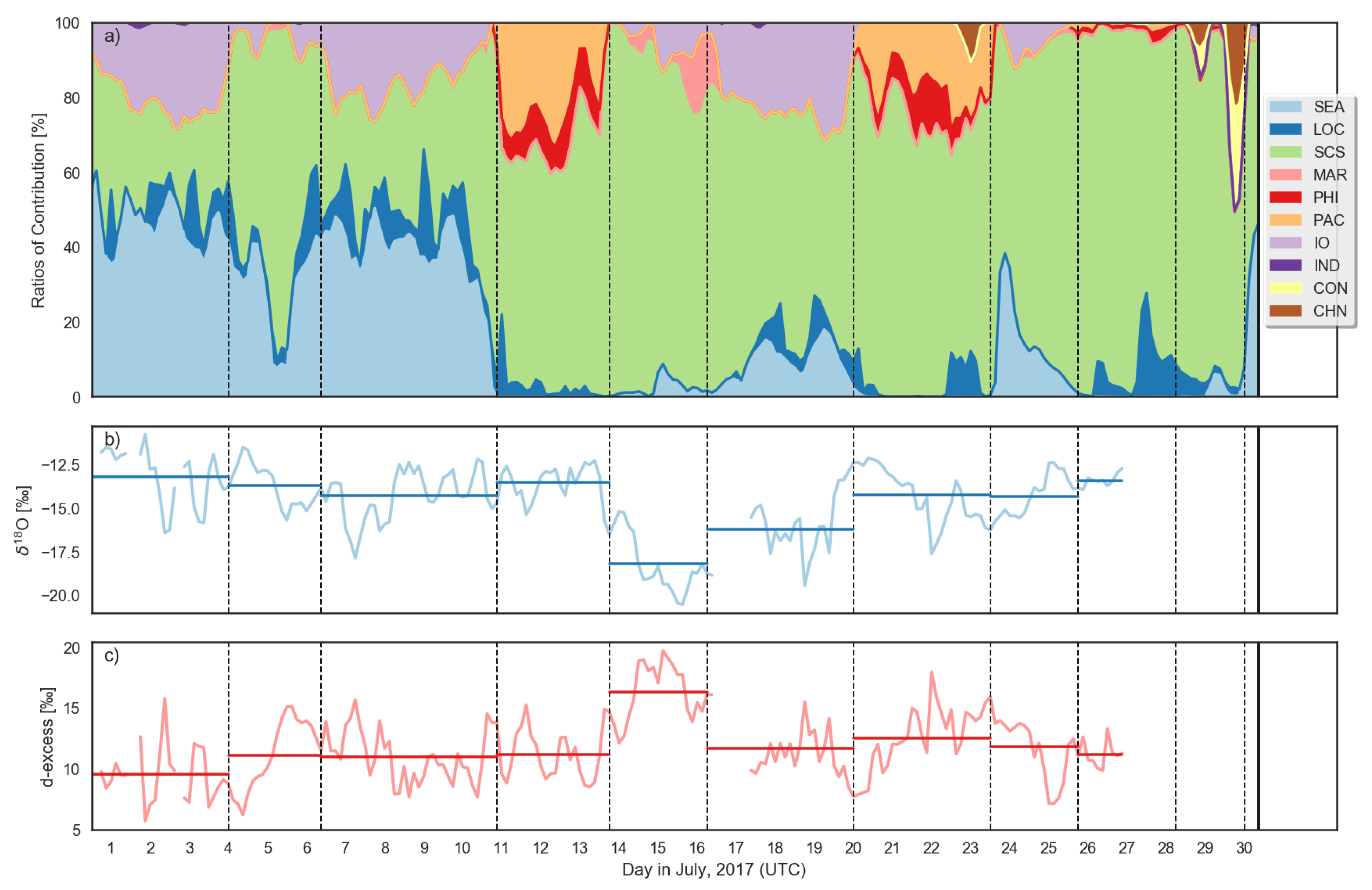
To further study the relationship between atmospheric transport and the isotopic composition of near-surface water vapor, Figure 11 shows the evolution of relative moisture contributions together with time series of observed ${\delta }^{18}$O and d-excess. The relative contributions the different moisture source domains varied substantially during July 2017, generally on time scales of 2 to 5 days. Although contributions from the South China Sea (SCS) were consistently large (from ∼20% to 100%), there was systematic co-variability among several of the other key source regions. For example, when contributions from mainland Southeast Asia (SEA) were large, contributions from the Indian Ocean also tended to be large. By contrast, when contributions from SEA were small, contributions from the Philippine Islands and Pacific Ocean were enhanced. These differences indicate shifts in the dominant direction of the low-level flow, from southwesterly (SEA and IO) to southeasterly (PHI and PAC). A shift in the low-level flow from southwesterly to southeasterly might be expected to correspond to an increase in heavy isotopic ratios due to the potential for enhanced rainout as air traverses the Southeast Asian highlands en route from the Indian Ocean to Gaoqiao (in contrast to flow from the Pacific, which is less likely to experience orographic uplift). Such an increase in ${\delta }^{18}$O was observed around day 20 when the prevailing flow shifted from southwesterly to southeasterly; however, no significant increase was observed around day 11 when the same type of southwesterly-to-southeasterly shift occurred. Additional measurements covering a longer period will be needed to constrain the isotopic signatures of these shifts in the prevailing large-scale circulation patterns.

The extremely large relative moisture contributions (80–100%) from the SCS on days 14–16 were associated with the passage of Tropical Storm Talas to the south of the observation site. The influence of this tropical cyclone manifested as a sharp decrease in ${\delta }^{18}$O and a sharp increase in d-excess in water vapor at the Gaoqiao site, with both quantities reaching their extreme values during the observation period. A series of large precipitation events associated with the outer regions of this typhoon passed over the observation site around this time. These features are discussed in detail in the following section.

6. Tropical Storm Talas

Days 14, 15, and 16 in Figure 11 (UTC) roughly correspond to 15–17 July LST, when Tropical Storm Talas passed over a portion of the South China Sea not far from the Gaoqiao site. Afternoon thunderstorms were common on the days leading up to the passage of the tropical storm, including 13–15 July. By contrast, rainfall on 16 July was intermittent throughout the day. We observed a total of 12 rainfall events and collected six rain samples on this day, associated with a cumulative daily rainfall amount that far exceeded the amounts observed on other dates in July 2017. However, the intensity of the rainfall associated with these six events was not large. The lack of afternoon thunderstorms, otherwise a near-daily occurrence during the campaign, continued through 17 and 18 July. This difference illustrates the extent to which the large-scale circulation pattern associated with the tropical storm perturbed the local meteorological conditions. This type of large-scale influence can perhaps be seen more intuitively in changes of the isotopic content of water vapor. Unfortunately, an extended power outage on the morning of 17 July interrupted the operation of the Picarro CRDS instrument. Owing to the resulting lack of observational data on 17 July, we restrict our analysis to 15–16 July.

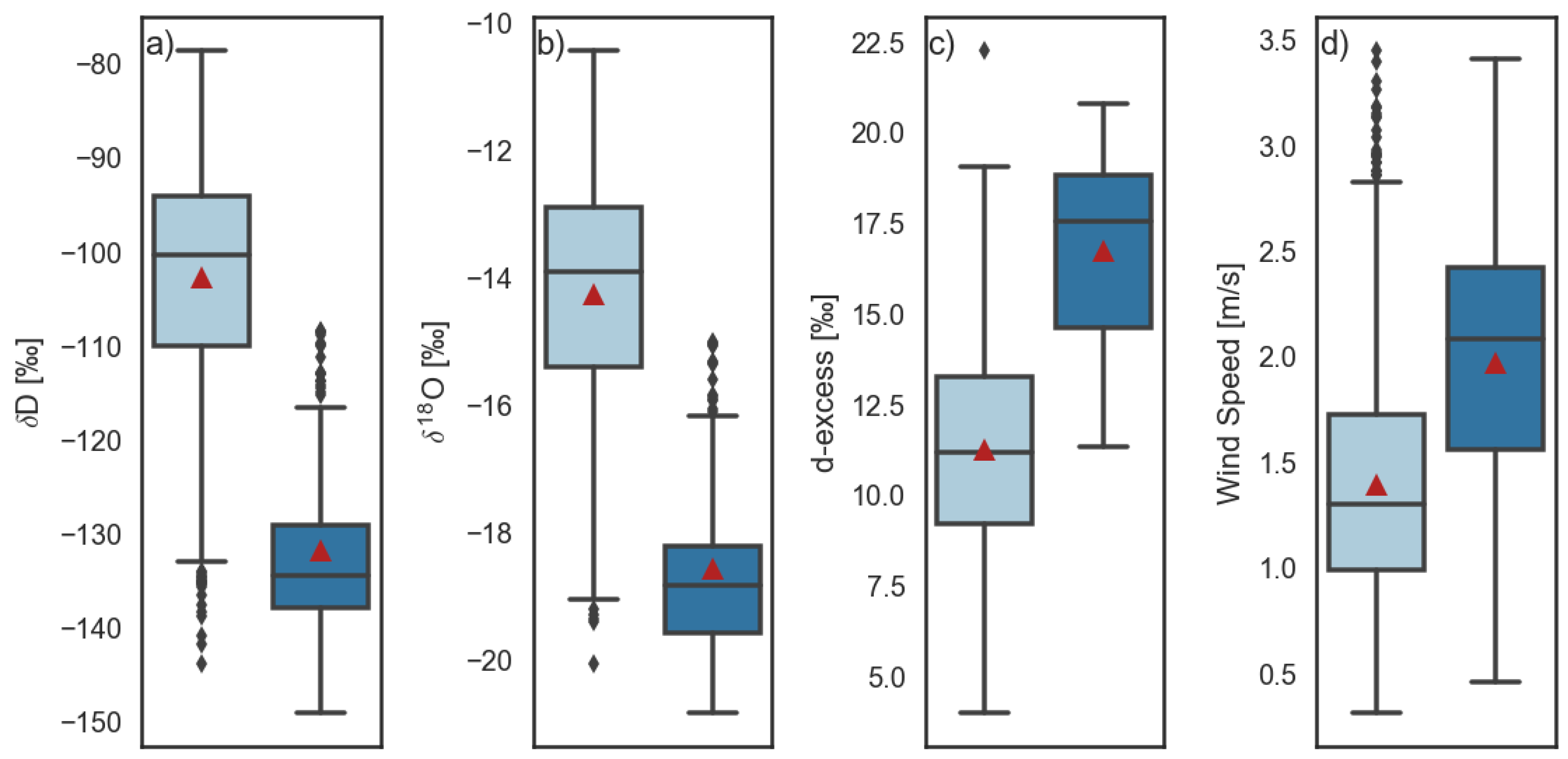
The values of ${\delta }^{18}$O and $\delta$D in water vapor observed on 15 and 16 July were systematically less than those oberved on other dates, while d-excess was systematically larger. Rainwater collected on these dates was likewise depleted of heavy isotopologues relative to almost all other samples we collected. To better illustrate these differences, Figure 12 shows key differences between the data collected on 15–16 July and the data collected on other dates during the campaign. Values of $\delta$D were reduced by 30∼35% on 15 and 16 July. Values of ${\delta }^{18}$O were similarly reduced by 4∼5%, while average values of d-excess were more than 5% higher than on other days. Figure 12d shows that average local wind speeds were also larger on 15–16 July than those observed on other days.

The changes shown in Figure 12 are consistent with an increased influence of kinetic fractionation due to rain–vapor exchange associated with intense deep convection during 15 and 16 July. However, no strong storms occurred directly at the site. Therefore, these effects were likely associated with large-scale transport of water vapor processed by deep convection elsewhere.

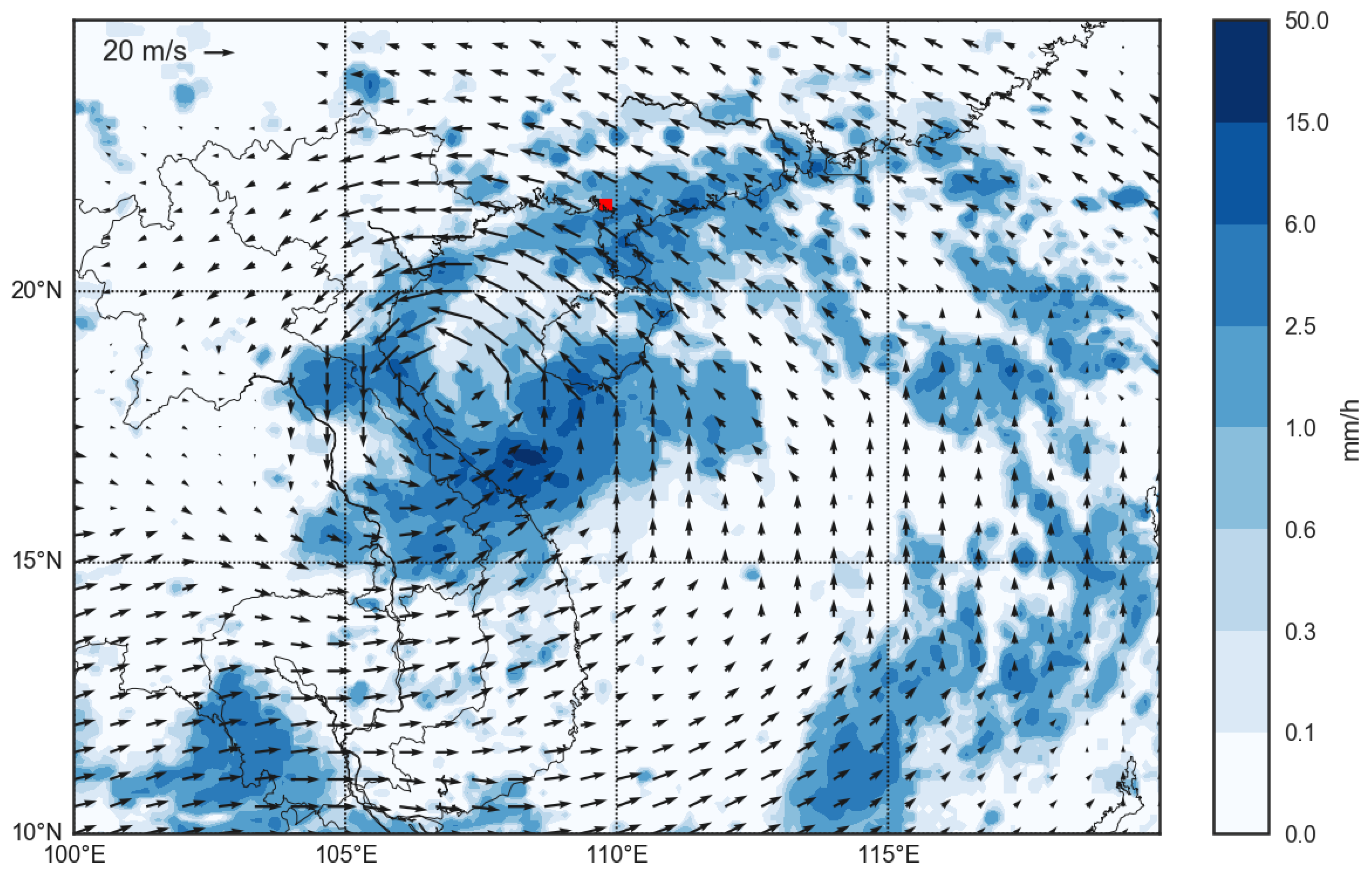
To further examine this possibility, Figure 13 shows the spatial distributions of precipitation and lower tropospheric winds on 16 July. The precipitation data are based on the Global Precipitation Measurement (GPM) Integrated Multi-satellitE Retrievals for GPM (IMERG) satellite-based data product [50]. Data are provided every 30 min on a ${0.1}^{\circ }\times {0.1}^{\circ }$ grid. The lower tropospheric wind field is based on the Modern-Era Retrospective Analysis for Research and Applications, Version 2 (MERRA-2) reanalysis [51,52] on the 850 hPa isobaric surface. These distributions provide a snapshot of Tropical Storm Talas as it propagated along a southeast-to-northwest track between Hainan Island and mainland Southeast Asia. Although the center of this tropical cyclone did not pass directly over the site, a series of rainfall events associated with the outer bands of the storm did extend northward to Gaoqiao and beyond.

The circulation associated with Tropical Storm Talas provided large amounts of moisture to the Gaoqiao site as the storm approached Southeast Asia. Previous studies have shown that heavy isotopic ratios in water vapor and rainfall associated with tropical storms and typhoons gradually decrease from the outer edges of the storm toward the center, with the exception of a pronounced maximum near the center of the storm, under the eyewall [9,53]. The latter is associated with isotopic enrichment caused by the evaporation of sea spray near the radius of maximum winds [9], and did not directly impact our measurements. Nor can we speak directly to the gradient in isotopic ratios along the radial axis of the storm, as our observations only sampled the outer bands along its northeastern edge. However, isotopic ratios in water vapor and rainfall were systematically reduced on 15 and 16 July, when the outer bands of Tropical Storm Talas passed over the site, relative to other times during the observation period. The isotope ratios then increase as the influence of the tropical cyclone wanes, although the timing and rate of this change are obscured by the power outage that occurred on 17 July. The reduced isotopic ratios and enhanced d-excess in the outer bands of large cyclones such as Talas are consistent with extensive isotopic distillation (formation and rainout of large amounts of rainfall) and kinetic isotopic exchange between vapor and rainfall in relatively dry air. The latter implies extensive evaporative moistening of air with low relative humidity in convective downdrafts [45]. Moisture convergence that extends deep into the free atmosphere to levels where $\delta$D and ${\delta }^{18}$O in water vapor are typically smaller may also play a role [48].

7. Summary

We have presented high-resolution measurements of isotopic ratios in surface-layer water vapor collected at the Gaoqiao Mangrove Reserve in southern China over multiple weeks in July 2017. These measurements of the stable isotopic composition of water vapor are supported by observations of isotopic ratios in precipitation, measurements of core meteorological variables collected at a nearby flux tower, and back trajectory analyses.

A high correlation between rainfall and vapor isotopic observation indicates substantial exchange between water vapor and raindrops falling through the boundary layer. Comparison with theoretical estimates based on thermodynamic equilibrium suggest that both equilibrium and kinetic fractionation processes contribute to this exchange. The average observed isotopic ratios are consistent with isotopic exchange occurring at a temperature of 27${}^{\circ }$C and a relative humidity of 87%, assuming that the equilibration time is sufficiently long relative to the time it takes for raindrops to transit the well-mixed surface layer. These estimates are similar to the average values observed during rainfall events (27${}^{\circ }$C and 90%, respectively). The extent of isotopic disequilibrium between rainfall and water vapor varied considerably among the rain events observed during the study period.

Further examination of the observed evolution of isotopic ratios during rainfall events identifies two types of rainfall events that occurred during the observation period. The first type (referred to as type A in the text) represents large-scale organized convective systems, and is associated with decreasing values of ${\delta }^{18}$O and specific humidity and temporary increases in d-excess. The second type (referred to as type B) is more consistent with isolated, local convective events, and is characterized by increasing values of ${\delta }^{18}$O and specific humidity and decreasing values of d-excess. These observations indicate that kinetic fractionation associated with the partial evaporation of liquid droplets in unsaturated air is enhanced in type A events relative to type B events. Plausible explanations for these isotopic differences include stronger and more frequent downdrafts during large-scale (type A) events, a systematically more humid boundary layer during local (type B) events, or some combination thereof.

A moisture source attribution based on back trajectories indicates that approximately 75% of the moisture is contributed by oceanic sources, with the remaining 25% contributed by continental sources. The oceanic sources were dominated by the nearby South China Sea ($\sim 63\%$ of the total moisture source), with secondary contributions from the Indian Ocean ($\sim 9\%$; via Southeast Asia) and Pacific Ocean ($\sim 4\%$; via the Luzon Strait and the Philippines). The primary continental moisture source (and second most influential overall) was mainland Southeast Asia ($\sim 16\%$), with local land areas contributing almost all of the remainder ($\sim 5\%$). Together, these five regions accounted for more than 96% of the attributable moisture source.

On 15–17 July, near the middle of the observation period, Tropical Storm Talas passed through the South China Sea to the south of the Gaoqiao mangrove measurement site. The passage of this storm dramatically reduced the isotopic composition of water vapor over those several days. The isotopic signatures are consistent with extensive isotopic distillation and rain–vapor exchange in the outer rain bands of the tropical cyclone. Back trajectory analysis indicates that the South China Sea was the source of almost all of the moisture at Gaoqiao during this period.

Our observations help to illuminate the role of atmospheric processes in isotopic water cycling above the Gaoqiao mangrove, including rain–vapor exchange and large-scale transport. The isotopic ratios examined in this work are valuable tracers of the exchanges of water among the atmosphere, ocean, vegetation, and soils in coastal regions. However, the short length of the data record limits the generalizability of our results. Further observations covering longer periods, multiple seasons, and a greater range of weather systems are now being collected in an ongoing effort to continue improving our understanding of the water and carbon cycles in this economically and ecologically important coastal ecosystem.

References

1. Galewsky, J.; Steen-Larsen, H.C.; Field, R.D.; Worden, J.; Risi, C.; Schneider, M. Stable isotopes in atmospheric water vapor and applications to the hydrologic cycle. Rev. Geophys. 2016, 54, 809–865. [Google Scholar] [CrossRef] [Green Version]
2. Craig, H. Isotopic variations in meteoric waters. Science 1961, 133, 1702–1703. [Google Scholar] [CrossRef] [PubMed]
3. Dansgaard, W. Stable isotopes in precipitation. Tellus 1964, 16, 436–468. [Google Scholar] [CrossRef]
4. Risi, C.; Bony, S.; Vimeux, F.; Frankenberg, C.; Noone, D.; Worden, J. Understanding the Sahelian water budget through the isotopic composition of water vapor and precipitation. J. Geophys. Res. Atmos. 2010, 115, D24. [Google Scholar] [CrossRef]
5. Noone, D.; Galewsky, J.; Sharp, Z.D.; Worden, J.; Barnes, J.; Baer, D.; Bailey, A.; Brown, D.P.; Christensen, L.; Crosson, E.; et al. Properties of air mass mixing and humidity in the subtropics from measurements of the D/H isotope ratio of water vapor at the Mauna Loa Observatory. J. Geophys. Res. Atmos. 2011, 116, 898–908. [Google Scholar] [CrossRef]
6. Kurita, N.; Fujiyoshi, Y.; Nakayama, T.; Matsumi, Y.; Kitagawa, H. East Asian Monsoon controls on the inter-annual variability in precipitation isotope ratio in Japan. Clim. Past 2015, 11, 339. [Google Scholar] [CrossRef]
7. Tremoy, G.; Vimeux, F.; Soumana, S.; Souley, I.; Risi, C.; Favreau, G.; Oï, M. Clustering mesoscale convective systems with laser-based water vapor δ18O monitoring in Niamey (Niger). J. Geophys. Res. Atmos. 2014, 119, 5079–5103. [Google Scholar] [CrossRef]
8. Conroy, J.L.; Noone, D.; Cobb, K.M.; Moerman, J.W.; Konecky, B.L. Paired stable isotopologues in precipitation and vapor: A case study of the amount effect within western tropical Pacific storms. J. Geophys. Res. Atmos. 2016, 121, 3290–3303. [Google Scholar] [CrossRef]
9. Fudeyasu, H.; Ichiyanagi, K.; Sugimoto, A.; Yoshimura, K.; Ueta, A.; Yamanaka, M.; Ozawa, K. Isotope ratios of precipitation and water vapor observed in Typhoon Shanshan. J. Geophys. Res. Atmos. 2008, 113, D12. [Google Scholar] [CrossRef]
10. Steen-Larsen, H.; Sveinbjörnsdottir, A.; Jonsson, T.; Ritter, F.; Bonne, J.L.; Masson-Delmotte, V.; Sodemann, H.; Blunier, T.; Dahl-Jensen, D.; Vinther, B. Moisture sources and synoptic to seasonal variability of North Atlantic water vapor isotopic composition. J. Geophys. Res. Atmos. 2015, 120, 5757–5774. [Google Scholar] [CrossRef] [Green Version]
11. Li, J.; Tao, T.; Pang, Z.; Tan, M.; Kong, Y.; Duan, W.; Zhang, Y. Identification of different moisture sources through isotopic monitoring during a storm event. J. Hydrometeorol. 2015, 16, 1918–1927. [Google Scholar] [CrossRef]
12. Bonne, J.L.; Masson-Delmotte, V.; Cattani, O.; Delmotte, M.; Risi, C.; Sodemann, H.; Steen-Larsen, H. The isotopic composition of water vapour and precipitation in Ivittuut, southern Greenland. Atmos. Chem. Phys. 2014, 14, 4419–4439. [Google Scholar] [CrossRef]
13. Krklec, K.; Domínguez-Villar, D. Quantification of the impact of moisture source regions on the oxygen isotope composition of precipitation over Eagle Cave, central Spain. Geochim. Cosmochim. Acta 2014, 134, 39–54. [Google Scholar] [CrossRef]
14. Galewsky, J.; Samuels-Crow, K. Water vapor isotopic composition of a stratospheric air intrusion: Measurements from the Chajnantor Plateau, Chile. J. Geophys. Res. Atmos. 2014, 119, 9679–9691. [Google Scholar] [CrossRef] [Green Version]
15. Alongi, D.M. Mangrove forests: Resilience, protection from tsunamis, and responses to global climate change. Estuar. Coast. Shelf Sci. 2008, 76, 1–13. [Google Scholar] [CrossRef]
16. Bouillon, S.; Connolly, R.; Lee, S. Organic matter exchange and cycling in mangrove ecosystems: recent insights from stable isotope studies. J. Sea Res. 2008, 59, 44–58. [Google Scholar] [CrossRef] [Green Version]
17. Cui, X.; Liang, J.; Lu, W.; Chen, H.; Liu, F.; Lin, G.; Xu, F.; Luo, Y.; Lin, G. Stronger ecosystem carbon sequestration potential of mangrove wetlands with respect to terrestrial forests in subtropical China. Agric. For. Meteorol. 2018, 249, 71–80. [Google Scholar] [CrossRef]
18. Valiela, I.; Bowen, J.L.; York, J.K. Mangrove Forests: One of the World’s Threatened Major Tropical Environments: At least 35% of the area of mangrove forests has been lost in the past two decades, losses that exceed those for tropical rain forests and coral reefs, two other well-known threatened environments. Bioscience 2001, 51, 807–815. [Google Scholar]
19. Chen, L.; Wang, W.; Zhang, Y.; Lin, G. Recent progresses in mangrove conservation, restoration and research in China. J. Plant Ecol. 2009, 2, 45–54. [Google Scholar] [CrossRef] [Green Version]
20. Liang, J.; Wright, J.S.; Cui, X.; Sternberg, L.; Gan, W.; Lin, G. Leaf anatomical traits determine the 18O enrichment of leaf water in coastal halophytes. Plant Cell Environ. 2018. [Google Scholar] [CrossRef] [PubMed]
21. Twilley, R.R.; Chen, R. A water budget and hydrology model of a basin mangrove forest in Rookery Bay, Florida. Mar. Freshw. Res. 1998, 49, 309–323. [Google Scholar] [CrossRef]
22. Schaeffer-Novelli, Y.; Cintrón-Molero, G.; Adaime, R.R.; de Camargo, T.M. Variability of mangrove ecosystems along the Brazilian coast. Estuaries 1990, 13, 204–218. [Google Scholar] [CrossRef]
23. Majoube, M. Fractionation in O-18 between ice and water vapor. J. Chim. Phys. Phys.-Chim. Biol. 1971, 68, 625–636. [Google Scholar] [CrossRef]
24. Merlivat, L.; Jouzel, J. Global climatic interpretation of the deuterium-oxygen 18 relationship for precipitation. J. Geophys. Res. Oceans 1979, 84, 5029–5033. [Google Scholar] [CrossRef]
25. Bonne, J.L.; Steen-Larsen, H.C.; Risi, C.; Werner, M.; Sodemann, H.; Lacour, J.L.; Fettweis, X.; Cesana, G.; Delmotte, M.; Cattani, O.; et al. The summer 2012 Greenland heat wave: In situ and remote sensing observations of water vapor isotopic composition during an atmospheric river event. J. Geophys. Res. Atmos. 2015, 120, 2970–2989. [Google Scholar] [CrossRef] [Green Version]
26. Welp, L.R.; Lee, X.; Griffis, T.J.; Wen, X.F.; Xiao, W.; Li, S.; Sun, X.; Hu, Z.; Val Martin, M.; Huang, J. A meta-analysis of water vapor deuterium-excess in the midlatitude atmospheric surface layer. Glob. Biogeochem. Cycles 2012, 26. [Google Scholar] [CrossRef] [Green Version]
27. Simonin, K.A.; Link, P.; Rempe, D.; Miller, S.; Oshun, J.; Bode, C.; Dietrich, W.E.; Fung, I.; Dawson, T.E. Vegetation induced changes in the stable isotope composition of near surface humidity. Ecohydrology 2014, 7, 936–949. [Google Scholar] [CrossRef]
28. Fiorella, R.P.; Bares, R.; Lin, J.C.; Ehleringer, J.R.; Bowen, G.J. Detection and variability of combustion-derived vapor in an urban basin. Atmos. Chem. Phys. 2018, 18, 8529–8547. [Google Scholar] [CrossRef]
29. Fiorella, R.P.; Poulsen, C.J.; Matheny, A.M. Seasonal patterns of water cycling in a deep, continental mountain valley inferred from stable water vapor isotopes. J. Geophys. Res. Atmos. 2018. [Google Scholar] [CrossRef]
30. Benetti, M.; Reverdin, G.; Pierre, C.; Merlivat, L.; Risi, C.; Steen-Larsen, H.C.; Vimeux, F. Deuterium excess in marine water vapor: Dependency on relative humidity and surface wind speed during evaporation. J. Geophys. Res. Atmos. 2014, 119, 584–593. [Google Scholar] [CrossRef] [Green Version]
31. Noone, D. Pairing Measurements of the Water Vapor Isotope Ratio with Humidity to Deduce Atmospheric Moistening and Dehydration in the Tropical Midtroposphere. J. Clim. 2012, 25, 4476–4494. [Google Scholar] [CrossRef]
32. Steen-Larsen, H.C.; Johnsen, S.J.; Masson-Delmotte, V.; Stenni, B.; Risi, C.; Sodemann, H.; Balslev-Clausen, D.; Blunier, T.; Dahl-Jensen, D.; Ellehøj, M.; et al. Continuous monitoring of summer surface water vapor isotopic composition above the Greenland Ice Sheet. Atmos. Chem. Phys. 2013, 13, 4815–4828. [Google Scholar] [CrossRef] [Green Version]
33. Stohl, A.; Forster, C.; Frank, A.; Seibert, P.; Wotawa, G. The Lagrangian particle dispersion model FLEXPART version 6.2. Atmos. Chem. Phys. 2005, 5, 2461–2474. [Google Scholar] [CrossRef]
34. Spichtinger, N.; Wenig, M.; James, P.; Wagner, T.; Platt, U.; Stohl, A. Satellite detection of a continental-scale plume of nitrogen oxides from boreal forest fires. Geophys. Res. Lett. 2001, 28, 4579–4582. [Google Scholar] [CrossRef] [Green Version]
35. Damoah, R.; Spichtinger, N.; Forster, C.; James, P.; Mattis, I.; Wandinger, U.; Beirle, S.; Wagner, T.; Stohl, A. Around the world in 17 days-hemispheric-scale transport of forest fire smoke from Russia in May 2003. Atmos. Chem. Phys. 2004, 4, 1311–1321. [Google Scholar] [CrossRef]
36. Stohl, A.; James, P. A Lagrangian analysis of the atmospheric branch of the global water cycle. Part I: Method description, validation, and demonstration for the August 2002 flooding in central Europe. J. Hydrometeorol. 2004, 5, 656–678. [Google Scholar] [CrossRef]
37. Sodemann, H.; Schwierz, C.; Wernli, H. Interannual variability of Greenland winter precipitation sources: Lagrangian moisture diagnostic and North Atlantic Oscillation influence. J. Geophys. Res. Atmos. 2008, 113. [Google Scholar] [CrossRef] [Green Version]
38. Dee, D.P.; Uppala, S.M.; Simmons, A.J.; Berrisford, P.; Poli, P.; Kobayashi, S.; Andrae, U.; Balmaseda, M.A.; Balsamo, G.; Bauer, P. The ERA-Interim reanalysis: configuration and performance of the data assimilation system. Q. J. R. Meteorol. Soc. 2011, 137, 553–597. [Google Scholar] [CrossRef] [Green Version]
39. Huang, W.; He, X.; Yang, Z.; Qiu, T.; Wright, J.S.; Wang, B.; Lin, D. Moisture sources for wintertime extreme precipitation events over South China during 1979–2013. J. Geophys. Res. Atmos. 2018, 123, 6690–6712. [Google Scholar] [CrossRef]
40. Trenberth, K.E.; Stepaniak, D.P. Covariability of components of poleward atmospheric energy transports on seasonal and interannual timescales. J. Clim. 2003, 16, 3691–3705. [Google Scholar] [CrossRef]
41. Risi, C.; Noone, D.; Frankenberg, C.; Worden, J. Role of continental recycling in intraseasonal variations of continental moisture as deduced from model simulations and water vapor isotopic measurements. Water Resour. Res. 2013, 49, 4136–4156. [Google Scholar] [CrossRef] [Green Version]
42. Yoshimura, K.; Kanamitsu, M.; Noone, D.; Oki, T. Historical isotope simulation using reanalysis atmospheric data. J. Geophys. Res. Atmos. 2008, 113. [Google Scholar] [CrossRef]
43. Kurita, N. Water isotopic variability in response to mesoscale convective system over the tropical ocean. J. Geophys. Res. Atmos. 2013, 118. [Google Scholar] [CrossRef]
44. Lee, J.E.; Fung, I. “Amount effect” of water isotopes and quantitative analysis of post-condensation processes. Hydrol. Proc. 2008, 22, 1–8. [Google Scholar] [CrossRef]
45. Risi, C.; Bony, S.; Vimeux, F. Influence of convective processes on the isotopic composition (δ18O and δD) of precipitation and water vapor in the tropics: 2. Physical interpretation of the amount effect. J. Geophys. Res. Atmos. 2008, 113. [Google Scholar] [CrossRef]
46. Stewart, M.K. Stable isotope fractionation due to evaporation and isotopic exchange of falling waterdrops: Applications to atmospheric processes and evaporation of lakes. J. Geophys. Res. 1975, 80, 1133–1146. [Google Scholar] [CrossRef]
47. Bony, S.; Risi, C.; Vimeux, F. Influence of convective processes on the isotopic composition (δ18O and δD) of precipitation and water vapor in the tropics: 1. Radiative-convective equilibrium and Tropical Ocean–Global Atmosphere–Coupled Ocean-Atmosphere Response Experiment (TOGA-COARE) simulations. J. Geophys. Res. Atmos. 2008, 113. [Google Scholar] [CrossRef]
48. Moore, M.; Kuang, Z.; Blossey, P.N. A moisture budget perspective of the amount effect. Geophys. Res. Lett. 2014, 41, 1329–1335. [Google Scholar] [CrossRef] [Green Version]
49. Van der Ent, R.J.; Savenije, H.H.; Schaefli, B.; Steele-Dunne, S.C. Origin and fate of atmospheric moisture over continents. Water Resour. Res. 2010, 46. [Google Scholar] [CrossRef] [Green Version]
50. Huffman, G.; Bolvin, D.; Braithwaite, D.; Hsu, K.; Joyce, R.; Xie, P. GPM IMERG Final Precipitation L3 Half Hourly 0.1 Degree x 0.1 Degree V05 [Data Set]; NASA’s Precipitation Processing Center, NASA GSFC: Greenbelt, MD, USA, 2017. [CrossRef]
51. Gelaro, R.; McCarty, W.; Suárez, M.J.; Todling, R.; Molod, A.; Takacs, L.; Randles, C.A.; Darmenov, A.; Bosilovich, M.G.; Reichle, R.; et al. The Modern-Era Retrospective Analysis for Research and Applications, Version 2 (MERRA-2). J. Clim. 2017, 30, 5419–5454. [Google Scholar] [CrossRef]
52. Global Modeling and Assimilation Office. MERRA-2 tavg1_2d_slv_Nx: 2d, 1-Hourly, Time-Averaged, Single-Level, Assimilation, Single-Level Diagnostics V5.12.4 [Data Set]; NASA Goddard Earth Sciences Data and Information Services Center (GES DISC): Greenbelt, MD, USA, 2015. [CrossRef]
53. Munksgaard, N.C.; Zwart, C.; Kurita, N.; Bass, A.; Nott, J.; Bird, M.I. Stable isotope anatomy of tropical cyclone Ita, North-Eastern Australia, April 2014. PLoS ONE 2015, 10, e0119728. [Google Scholar] [CrossRef] [PubMed]
Figure 1. Location of the Gaoqiao Mangrove Reserve measurement site and the building where measurements were collected.
Atmosphere 09 00365 g001
Figure 2. Data measured during the July 2017 campaign at Gaoqiao Mangrove Reserve by the Piccaro L2130-i water vapor isotopic analyzer (upper four panels) and by the nearby weather station (lower four panels). Shaded areas mark the transitions between days (midnight to midnight local time). The ∼1-day data gap in the middle was caused by an extended power outage. A wind direction of 0 corresponds to winds from the north.
Atmosphere 09 00365 g002
Figure 3. Distributions of (a) δ D and (b) d-excess against δ 18 O in measurements of near-surface water vapor at Gaoqiao mangrove during July 2017. The red lines indicate linear fits to the measurements based on ordinary least squares. The blue line in panel (a) indicates the canonical global meteoric water line (GMWL).
Atmosphere 09 00365 g003
Figure 4. Distribution of δ D relative to specific humidity (q). Darker hexagons in the central axis indicate greater joint densities. The dotted line traces the Rayleigh distillation curve (Equation (4)) starting from δ D = 80 % and q = 25 g kg 1 . The solid lines indicate mixing lines (Equation (5)) between a ‘moist’ air mass with δ D = 80 % and q = 25 g kg 1 and a ‘dry’ air mass with q = 9.3 g kg 1 and δ D values of (from top to bottom) 110 %, 120 %, 130 %, 140 %, 150 %, and 160 %. Settings for the theoretical models are based on outputs from an isotope-enabled global model [42] for water vapor at different vertical levels near the observation site.
Atmosphere 09 00365 g004
Figure 5. Comparison between theoretical equilibrium rainfall δ D (calculated based on observed vapor δ D and temperature) and observed rainfall δ D.
Atmosphere 09 00365 g005
Figure 6. Isotopic evolution during observed rainfall events. The red curve in each panel shows changes in vapor δ 18 O (ordinate) as a function of time (abscissa). The blue shading indicates the duration of the rainfall event, extended to the left and right to show changes in δ 18 O before and after rainfall, respectively. The range of the abscissa depends on the duration of the event as described in the text and noted on the corresponding panel. The ordinate corresponds to the anomaly in δ 18 O relative to the mean value over the plotted time range. The classification of each event (‘A’, ‘B’ or none as discussed in the text) is shown in the title of the corresponding panel.
Atmosphere 09 00365 g006
Figure 7. Comparison of type A and type B rainfall events with respect to (a) the duration of the event (unit: hr), (b) the cumulative rainfall amount (unit: mm), and (c) the associated rainfall rate (unit: mm hr 1 . The red triangle marks the mean, the center horizontal line marks the median, the upper and lower boundaries of the box contain the interquartile range, and the top and bottom of the vertical line represent the maximum and minimum values, excluding any outliers (grey diamonds).
Atmosphere 09 00365 g007
Figure 8. Anomalies relative to the respective daily mean for (a) δ D and (b) d-excess before (green), during (yellow), and after (purple) observed type A and type B rainfall events.
Atmosphere 09 00365 g008
Figure 9. The average relative contribution to surface-layer water vapor during the study period, projected onto a 1 × 1 grid.
Atmosphere 09 00365 g009
Figure 10. (a) Geographical partitioning of moisture source domains and (b) distributions of relative moisture contributions from each domain.
Atmosphere 09 00365 g010
Figure 11. Time evolution during July 2017 of (a) relative moisture source ratios for each region reconstructed using the FLEXPART model, (b) observed values of δ 18 O in water vapor at the Gaoqiao mangrove observation site, and (c) observed values of d-excess in water vapor at the same site.
Atmosphere 09 00365 g011
Figure 12. Observational data collected on 15 and 16 July (dark blue) relative to data collected on other days in July (light blue) for (a) δ D in water vapor, (b) δ 18 O in water vapor, (c) d-excess in water vapor, and (d) near-surface wind speed. Data were not collected on 17 July because of a power outage.
Atmosphere 09 00365 g012
Figure 13. Spatial distributions of precipitation based on GPM observations and lower tropospheric (850 hPa) horizontal winds based on the MERRA-2 reanalysis on 16 July 2017.
Atmosphere 09 00365 g013