Atmospheric Pollution by PM₁₀ and O₃ in the Guadalajara Metropolitan Area, Mexico

Abstract

To study the air quality in the Guadalajara Metropolitan Area (GMA), concentrations of suspended particles (PM₁₀) and ozone (O₃) reported by eight monitoring stations were analyzed. Also, six commonly found types of synoptic situations (TSS) during 1996–2016 were identified using an atmospheric pattern correlation method on the mean sea level pressure and geopotential heights (850 hPa, 500 hPa, and 200 hPa) of fields given by the North American Regional Reanalysis (NARR) database. Overall, 75% of the period of study was classified as one of the six TSS. Afterward, statistical significance tests (confidence level 95%) were applied to determine whether the TSS affected PM₁₀ and O₃ concentrations locally in the GMA. PM₁₀ maximum hourly concentrations (~76.7 μg/m³) occurred around 8 am local time, while that of ozone (~0.054 ppm) occurred between 1–4 pm local time. Meanwhile, PM₁₀ monthly levels were higher between December and May, and the highest O₃ concentrations occurred between April and June. Average annual levels of PM₁₀ have decreased through the years, while the annual trend of mean O₃ concentrations seemed to respond to the 11-year solar cycle. It was also found that during “convective-allowing situations” (TSS VI) and “thermal low over California” (TSS I), PM₁₀ concentrations remained low in the GMA, and O₃ concentrations rose under the influence of a “low-pressure system over the United States (USA)” (TSS II). Further research is suggested to address the effect of the local circulation in the GMA linked to the TSS on O₃ and PM₁₀ concentrations.

1. Introduction

High concentrations of air pollutants such as ozone (O₃) and suspended particles (PM₁₀) have a negative impact on the environment and human health (e.g., [1,2,3]). Guadalajara is the second most important city in Mexico regarding economic activity, territorial extension, and population density. According to the 2005 emission inventory [4] in the Guadalajara Metropolitan Area (GMA), 3.3 million tons of pollutants were emitted that year, of which 85.298% was carbon monoxide (CO), and 9.343% was volatile organic compounds (VOC). Nitrogen oxides (NO_x) accounted for 3.072% and PM₁₀ accounted for 0.556% of the total. The rest was represented by emissions of sulfur dioxide (SO₂), ammonia (NH₃), and PM_2.5. Furthermore, episodes of poor air quality in the GMA have been reported quite regularly [5,6] over the last years. It is also known that the pollutants that most frequently exceed air quality standards are O₃ and PM₁₀ [7].

The orographic conditions in the GMA actively influence its air quality. This city is located in the Valley of the Río Grande of Santiago watershed, between the Valley of Atemajac and the Tonalá plain; it is surrounded by natural barriers that limit the free flow of wind currents, and consequently, the dispersion of pollutants [8]. The mean elevation is 1566 m above mean sea level (AMSL). The GMA’s climate corresponds to a temperate, subtropical region that rains during the summer and is mostly dry during winter. The annual mean temperature is 19.3 °C with the lowest temperatures in January and the highest in May. The mean wind velocity is moderate in this region and mostly zonal; its mean direction varies from the east (E) in the rainy season to the west (W) during the dry season [8].

The air quality in the GMA has been poorly studied. However, the concentrations of criteria air pollutants have been measured continuously since 1996 in eight points of the city. To our knowledge, there is no published study that has used this database in its entirety, as all of the available research literature describes at most 11 years of these continuous measurements. One of the first works was carried out by Tereshchenko and Filonov [9], which analyzed the causes of one episode of high O₃ concentrations during October 1996. They found that the reason for such high ozone levels was the strong stability conditions over the GMA. The authors also recommended studying the synoptic patterns that most influenced the GMA in order to forecast episodes of high O₃ concentrations. Furthermore, Ramírez-Sánchez et al. [10] used observation data between 2000–2005 of the criteria pollutants (CO, SO₂, NO₂, PM₁₀, and O₃) to describe their spatio-temporal distribution. Here, only monthly averages were analyzed for the study period. One conclusion of this study is that no annual trend of PM₁₀ concentrations was observed during those years. Moreover, Benítez-García et al. [6] determined the behavior (hourly, seasonal, and annual) of these pollutants for the extended period 2000–2011. One of their findings was a definite tendency to increase annual O₃ mean concentrations. By a linear regression analysis between O₃ maximum levels and temperature, the authors suggested that another factor (besides temperature) should be relevant for such a trend. Finally, Kanda et al. [5] studied the formation of O₃ using the model WRF-CMAQ (Weather Research and Forecasting—Community Multiscale Air Quality), and found that in the GMA, the O₃ formation regimen is between VOC-sensitive and NO_x-sensitive regimes.

Air pollution emissions in industrial and urban areas, which are linked to weather conditions, can affect regional or even global scales (e.g., [11,12]). Meteorological conditions play an essential role in the formation, transformation, diffusion, transport, and removal of atmospheric pollutants [13,14,15]. Also, these conditions are determined by the synoptic scale and local factors. Due to this close relationship, many environmental studies [14,16,17] were conducted with the focus on how air quality behaves depending on the present type of synoptic situation (TSS). Currently, the most exhaustive classification of TSS for Mexico is that of Mosiño’s subjective weather types back in 1958 [18]. However, it is not possible to use this classification in the present work, since it requires an update, and also because its subjective character hinders its application for long periods of time (i.e., 21 years), as it is for the present study.

Therefore, the goal of this work is to analyze GMA air pollution and its link to regional weather conditions from 1996 to 2016 focusing on O₃ and PM₁₀ pollutants. This study is based on the hypothesis that the different TSS influence the average concentrations of O₃ and PM₁₀ in the GMA. Here, an updated classification of the different, and most common, types of synoptic situations (TSS) is performed. The strengths of the present investigation are that O₃ and PM₁₀ concentrations in the GMA are related to the most common TSS that affect this region, and that the air quality of the GMA is analyzed with a comprehensive, and updated dataset of these pollutants. Besides, the results that will be presented here constitute a useful tool for air quality forecasting in the GMA. To the best of our knowledge, this study is the first of its kind for this area.

After presenting the data and methodology used in this article in Section 2, Section 3.1 shows a temporal and spatial analysis of the PM₁₀ contaminant. Hourly, weekly, daily, monthly, and yearly mean concentration values are analyzed. In Section 3.2, a similar study is shown, but for the O₃ pollutant. Section 3.3 focuses on the classification of the TSS and the behavior of the PM₁₀ and O₃ concentrations for every one of them. Finally, the main conclusions are presented in Section 4.

2. Data and Methodology

In the present section, the area of study and the observation data used in this research are described. The classification method used to determine the most common types of synoptic situations is also explained. Furthermore, the analysis methods for O₃ and PM₁₀ pollutants are presented here.

2.1. Area of Study

The GMA is located in the State of Jalisco, Mexico, exactly in the Valley of the Río Grande de Santiago watershed, between the Valley of Atemajac and the Tonalá plain. Its mean altitude is around 1500 m AMSL, but it is surrounded by higher elevations. Also, the GMA is composed of five municipalities and is the second most populated city in Mexico, with 4.5 million inhabitants [19]. In addition, the GMA possesses a large vehicle fleet (mobile sources) that is responsible for 80% of the NO_x and 70% of the VOC emissions, while fixed point and area sources are responsible for 80% of the PM₁₀ emissions. Figure 1 shows the area of study.

Moreover, Figure 2a shows the average annual cycle of precipitation and temperature, and Figure 2b shows the diurnal cycle of temperature and mean wind speed for the GMA between 1996 and 2016. Figure 2c,d show the wind roses for the rainy and dry periods, respectively. The data from which Figure 2 was obtained was provided by the monitoring stations of the Jalisco Atmospheric Monitoring System (SIMAJ) and the Computerized Climate system (CLICOM by Spanish acronym). The details related to the data will be described in the following section. As it can be seen from Figure 2a, the rainy season starts in May and lasts until October, with a midsummer drought in August [20]. The maximum average daily precipitation occurs within June and July, with values higher than 9 mm/day. During the dry period, the average daily rainfall is less than 1 mm/day. Meanwhile, the maximum mean annual temperature is reached toward the end of the dry period (24.7 °C), and its minimum is in January (17.5 °C). The daily values in Figure 2b have a high correspondence with the height of the Sun in the sky. The minimum (~15 °C) is reached at the beginning of the solar day (6–7 am local time), while its maximum value (~27 °C) is attained in the afternoon (4–5 pm local time) when the Sun has already reached its zenith. Concerning the diurnal cycle of the wind speed, Figure 2b also shows a high correlation with temperature during the day. Prevailing wind directions vary from component E (with a frequency larger than 40% of cases) in the rainy season to component W (present over 45% of all cases) during the dry season; see Figure 2c,d This information agrees well with that provided by Davydova-Belitskaya et al. [8].

2.2. Observation Data

Eight monitoring stations from the SIMAJ are located in the study area that ensured the continuous monitoring of O₃ and PM₁₀ during the 1996–2016 period: Atemajac (Ate), Oblatos (Obl), Loma Dorada (Dor), Tlaquepaque (Tla), Miravalle (Mir), Las Aguilas (Agu), Vallarta (Val), and Centro (Cen); see Figure 1b. All of the air pollutants and meteorological data (temperature, wind speed, and wind direction) were gathered from these automatic stations. The O₃, PM₁₀, and meteorological data that was used in this study can be accessed at the web page [21] with one hour of temporal resolution. All of the information regarding these automatic stations was obtained from the Ministry of Environment and Territorial Development of Jalisco (SEMADET) through its web page [22]. In all of these stations, the ozone measurements were carried out by automatic analyzers (Ecotech, EC9810, Knoxfield, Australia) that use non-dispersive ultraviolet (UV) absorption technology (detection limit < 0.05 ppb), while the PM₁₀ data was acquired with Beta Continuous Particulate Monitors (Thermo Scientific, 5014i, Waltham, MA, USA) that use beta attenuation technology (detection limit < 1 μg/m³). With these sensors, the pollutant concentrations are reported hourly by averaging all of the measurements that were recorded in the time interval from 0 to 59 min within one hour, provided that at least 75% of the concentrations were recorded in that hour.

Table A1. Some additional details about the monitoring stations.

Station	Station Classification	Main Sources Near the Station	Surroundings Description
Atemajac (Ate)	Urban	Area sources	Residential and commercial area
Oblatos (Obl)	Urban	Area sources	Residential and commercial area
Loma Dorada (Dor)	Urban	Biogenic sources	Densely populated zone, few green areas
Tlaquepaque (Tla)	Urban	Area sources	Residential and commercial area with small pottery workshops
Miravalle (Mir)	Urban	Point sources	Industrial and residential area, no green areas
Las Aguilas (Agu)	Urban	Area sources	Residential area
Vallarta (Val)	Urban	Area sources	Residential zone with wooded areas
Centro (Cen)	Urban	Area sources	Commercial area with houses

shows some of the characteristics of the monitoring stations, of which seven are close to heavily trafficked roads. SIMAJ is ruled by the NOM-156-SEMARNAT-2012 norm, in which calibration, maintenance, and quality assurance/quality control procedures are established.

However, some additional quality controls were performed to identify missing, erroneous, and changes in the units of measurement of the data. Also, daily precipitation values have been obtained from CLICOM of the National Meteorological Service (NMS) available at this web page [23]. At the time of writing, the precipitation data available here corresponded to the period 1996–2014.

Furthermore, North American Regional Reanalysis (NARR) Data from the National Centers for Environmental Prediction (NCEP) have been obtained from this web page [24] to perform the classification of the TSS. These data cover all of North America (Canada, United States of America, and Mexico) with a spatial resolution of 32 km and a temporal resolution of 3 h. For the classification of the TSS, only a time resolution of 12 h (00 and 12 UTC) was used. NARR data was obtained and analyzed for the area shown in Figure 1a.

2.3. Methods

Since the amount of data from the eight monitoring stations is extensive, it was decided to analyze only the averages in the GMA. Thus, hourly, daily, weekly, monthly, and yearly mean values have been obtained by averaging the data from the eight monitoring stations. However, the spatial analysis has been performed using the data of each station, separately. All of the averages were calculated when there were at least 75% of the records necessary to determine each mean value independently of the temporal resolution, in agreement with Mexican standards. Missing data and outliers were excluded from all of the analyses. Reference concentration values from the NOM-020-SSA1-2014 and NOM-025-SSA1-2014 Mexican norms, and the World Health Organization (WHO) recommended limits (

Table A2. Air quality standards in Mexico and the World Health Organization (WHO) recommendations.

Pollutant	Sampling Time	Mexican Norm	WHO Recommendation
PM10 (μg/m3)	24 h	75.0	50.0
	1 year	40.0	20.0
O3 (ppm)	1 h	0.095	-
	8 h	0.070	0.050

) have been used to establish the air quality criteria. The 8-h moving averages of the O₃ concentrations were calculated following the recommendations of the NOM-020-SSA1-2014 norm.

The classification method used to identify the most common TSS in Mexico was the atmospheric pattern correlation method of Lund [25]. The variables used for the application of this semi-objective technique were the mean sea level pressure (pmsl) and the geopotential height at 850 hPa, 500 hPa, and 250 hPa. All of the 12-hourly maps from the NARR database were compared using linear correlation; every correlation coefficient obtained defined the similarity between the patterns. In this work, a correlation coefficient of 0.6 was used as criteria for grouping similar patterns. This correlation value is somewhat arbitrary but several experiments were performed with higher coefficients and the number of groups (or TSS) identified was too large. All of the maps that met the condition established by the correlation coefficient were grouped into a category. The categories with the higher number of members, after a long iterative process, were defined as key patterns, which were represented by the mean of their members. Once the main groups were obtained, a reclassification process was carried out in which each map in one group was compared with each of the key patterns. This procedure increased the similarities within each group and the differences between groups. In the end, a large number of maps were not related to any of the main selected groups, as they were representative of different transitional circulation patterns.

Furthermore, a one-way analysis of variance [26] of the averaged concentrations of O₃ and PM₁₀ associated with the TSS on the GMA was performed. Since there are several steps in the calculation of the variances between and within groups, it is common practice [27] to represent the entire group of results in a table known as the analysis of variance table (ANOVA;

Table 1. Analysis of Variance (ANOVA).

Source of Variation	Sums of Squares 1,2,3	Degrees of Freedom 4,5	Mean Square 6,7	F Ratio 8
Between groups	$S{C}_E={\displaystyle \sum }_{i=1}^k{n}_i{\left(\overline{y_i}-\overline{y}\right)}^2$	$k-1$	$S_E=\frac{S{C}_E}{k-1}$	$F_0=\frac{S_E}{S_D}$
Within groups	$S{C}_D={\displaystyle \sum }_{i=1}^k{\displaystyle \sum }_{j=1}^{n_j}{n}_i{\left(y_{ij}-\overline{y_i}\right)}^2$	$n-k$	$S_D=\frac{S{C}_D}{n-k}$
Total	$S{C}_{TOTAL}=S{C}_E+S{C}_D$	$n-1$

¹SC_E is the squared sum between groups, where $\overline{y}$ are mean values of O₃ and PM₁₀ for the whole study period (1996–2016); $\overline{y_i}$ is the corresponding mean for each type of synoptic situation (TSS). ² SC_D is the squared sum within groups; y_ij are the jth observations of the ith group. ³ SC_TOTAL is the total squared sum. ⁴ k is the number of groups (identified as TSS). ⁵ n is the number of observations of each pollutant. ⁶ S_E is the variance estimate between groups. ⁷ S_D is the variance estimate within groups. ⁸ F₀ is the test statistic.

). The comparison between the F ratio (Table 1) and an F critical value, as obtained from the Fisher probability density distribution with k − 1 degrees of freedom and n − k observations [28], would indicate whether at least one of the TSS has a statistically significant influence on the concentration of the pollutant in question. Afterward, a post-hoc analysis was realized using Tukey’s multiple comparisons method [29] to determine significant differences between O₃ and PM₁₀ mean pairs representing each TSS.

3. Results and Discussion

This section presents a temporal and spatial analysis for the pollutants of interest in this study (i.e., PM₁₀ and O₃). Also, the classification of the TSS, and their possible relation with PM₁₀ and O₃ concentrations in the GMA, are presented as well.

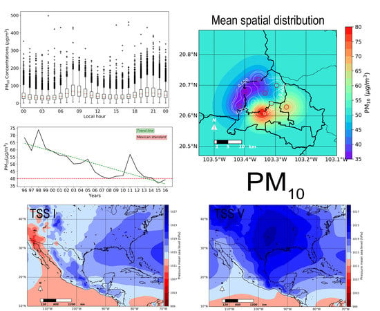
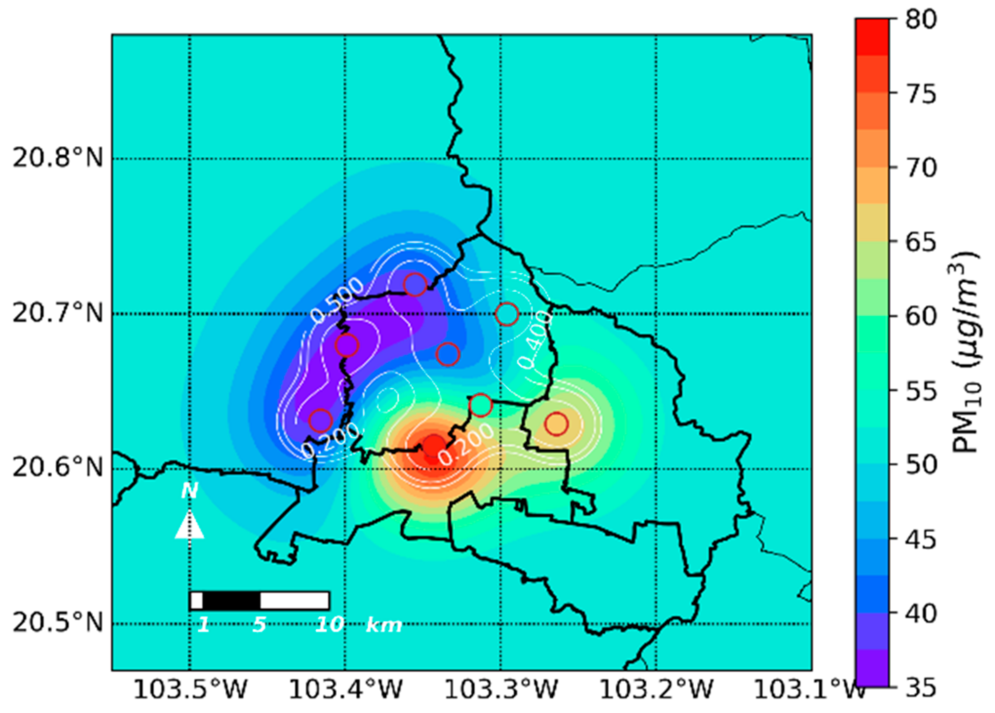
3.1. Temporal and Spatial Analysis of PM₁₀

Figure 3 shows the hourly (a), weekly (b), and daily (c) mean concentrations of PM₁₀ (in μg/m³) from the eight measurement stations for the study period. Figure 3a shows a bimodal feature of the PM₁₀ hourly mean concentrations. They oscillate around 50 μg/m³ with a minimum mean concentration of 32.89 μg/m³ at 4 am (local time). The first maximum of 76.61 μg/m³ is found at 8 am in the morning, while a secondary maximum is reported at 8 pm in the late afternoon. These peak hour schedules coincide with the hours of highest vehicular traffic when the PM₁₀ emissions rise. Also, the extreme values, shown with the plus sign in the figure, are found to reach up to 400 μg/m³.

From Figure 3b, it can be seen that PM₁₀ mean concentrations remain relatively high during weekdays and decrease on weekends as a consequence of the decay of the traffic and industrial activity at the end of the week [30]. The average daily concentrations of PM₁₀ in Figure 3c range around 50.13 μg/m³ with a standard deviation of 21.76 μg/m³ and extreme values as high as 173.79 μg/m³ and as low as 7.31 μg/m³. Such high variance makes that the Mexican standard and the amount recommended by the WHO for daily concentrations of PM₁₀ are frequently exceeded. One can also notice that these concentrations are related to the seasonal pattern, reaching the highest values in the dryer wintertime.

Furthermore, the monthly concentrations of PM₁₀ in Figure 4a begin to rise in October, reaching its maximum value in December and maintaining high amounts until May. This behavior is directly related to the rainy season in the GMA. From May to October, precipitations are more common; therefore, PM₁₀ concentrations remain low. During the period from November to April, PM₁₀ concentrations rise in correspondence with the time of low rainfall (see Figure 2a). A slight increase of these values in August can also be noted, which is related to the midsummer drought.

On the other hand, the annual average of PM₁₀ concentrations exceeds the Mexican annual standard from 1996 to 2014, as seen in Figure 4b. It is worth noting that the annual trend points to the decrease of the annual mean concentrations of PM₁₀, which could be related to the modernization of the vehicle fleet. Furthermore, a series of regulations on the quality of petroleum products have been implemented (NOM-016-CRE-2016 is the most recent one), as well as immediate contingency plans and mandatory vehicle verification programs [31]. Also note that Figure 4b shows a definite trend of decrease in the PM₁₀ concentrations, contrary to what Sánchez et al. [10] found for the period 2000–2005.

One of the most interesting features that Figure 4b shows is the peak of PM₁₀ concentrations reached during 2011. This peak was also observed for O₃ levels (see Section 3.2). This increase, of both pollutant concentrations, is related to a severe drought that affected the region from Nebraska in the United States (USA) to Central Mexico that year [32].

Figure A1 shows PM₁₀ and O₃ monthly concentrations anomalies; it also indicates monthly precipitation anomalies for 2011. Very high negative precipitation anomalies during the rainy season, especially, during June, August, and September can be observed in Figure A1. Consequently, PM₁₀ concentrations rose well above mean values during the following, more dry months (September–December). It is worth mentioning that these dryer-than-usual months typically increase forest fires in the region, which are a significant source of PM₁₀ during the dry season. It should also be worth mentioning that an extensive wooded area called Bosque de la Primavera is located on the immediate west of the GMA. The response for O₃ concentrations to precipitation is rather direct. The lesser the rainfall during the rainy season, the higher the O₃ levels during those months. In other words, as radiation is already favorable for ozone formation in the summertime (rainy season), the absence of precipitation during these same months increase the probability of finding O₃ concentrations higher than usual. During March, which is presented in Figure 2a as a month that is even dryer than February in the GMA, positive anomalies of PM₁₀ and O₃ were also found, which could be related (especially for PM₁₀) with February having registered a negative precipitation anomaly. However, note that positive anomalies of ozone concentrations were found for all of the months of that year.

Finally, Figure 5 shows the spatial behavior of the mean PM₁₀ concentrations in the GMA; the image was created using the objective mapping interpolation method with decorrelation scales, so the mean values on the measurement stations (red circles) are conserved. The errors associated with the interpolation method are shown in white solid lines. Here, it can be seen that the largest concentrations are located southeast of the city, which is where most of the point-emitting sources can be found [4]. Also, this part of the metropolis is less urbanized and keeps many unpaved roads. In contrast, the north and northwest regions report lower mean values of PM₁₀. This result agrees well with Ramírez-Sánchez et al. [10] in their analysis of pollutants in the GMA between 2000 and 2005.

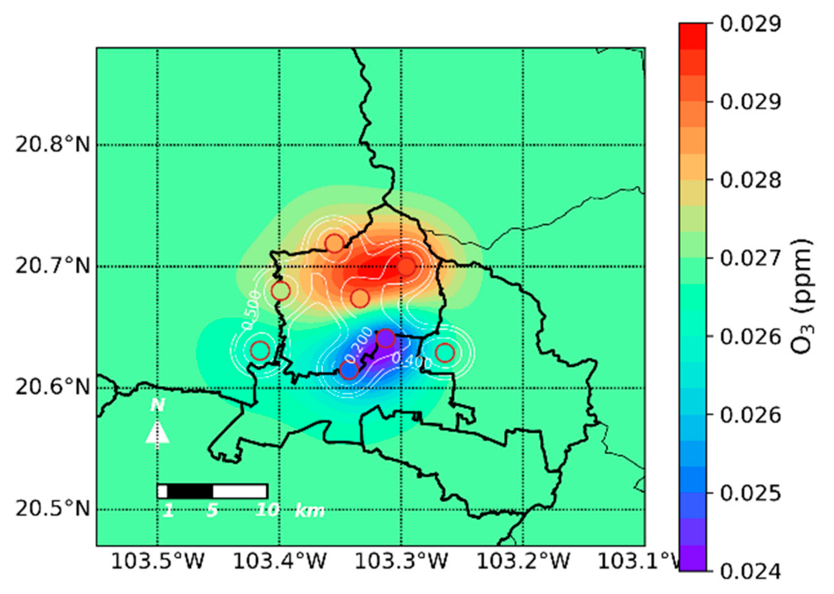
3.2. Temporal and Spatial Analysis of O₃

The average hourly concentrations of O₃ are shown in Figure 6a. They fluctuate around 0.026 ppm, while the maximum point values can exceed 0.175 ppm. It can be noted that higher mean O₃ values occur during the hours of higher solar radiation (1 pm to 4 pm), which coincide with the higher temperature intervals in Figure 2b. Also, the local minimum reached between 7–8 am is linked to the depletion of O₃ during the previous nighttime hours when the absence of the photochemical production of ozone and its destruction on solid surfaces prevail [6]. Although mean values remained slightly above 0.05 ppm between 1–4 pm, the maximum permissible of hourly concentrations of O₃, as established by the Mexican norm, were frequently exceeded.

Eight-hour mean ozone concentrations are calculated for each hour by averaging the observed O₃ level of the hour, and the values of the previous seven hours. Subsequently, the maximum concentration of all of these averages is determined for each year, and so it is reported as the eight-hour moving average of O₃ concentrations; see Figure 6c. In the 21-year period studied here, this variable appears to always exceed the established Mexican norm, excelling the year 1996 with the highest value. In this year, several particular episodes of very high concentrations of O₃ were reported [9].

Figure 6b presents the day-of-week average ozone and nitrogen dioxide concentrations in the GMA for the period of study. It might appear that the O₃ levels behave somewhat odd, since the bar chart shows two local maxima: a maximum during the weekdays and, let’s say, an unexpected peak during the weekend. The average concentrations of O₃ are above 0.0265 ppm during the weekdays and increase on the weekends, reaching their maximum mean value of the week (~0.0270 ppm) on Sundays. However, this behavior is known as the weekend effect [5,33,34,35]. This effect is produced because the formation of ozone is a highly non-linear process with the rates of production depending on the concentrations of its precursors (NO_x and VOC). Therefore, the weekend effect is often attributed to a reduction of 20% to 30% of the industrial activity and the flow of vehicles during the weekends, as compared with the weekdays, when the phenomenon is limited by VOC [36]. It can also be noted in Figure 6b that the NO₂ concentrations decrease drastically toward Sunday, which lets one believe that the excess of NO₂ on weekdays is keeping the ozone formation low. During the weekends, the NO_x concentration falls as the O₃ concentration rises. This result can be explained by the titration reaction (1). Kanda et al. [5] further explain this topic.

NO + O₃ → NO₂ + O₂

(1)

The monthly mean levels of O₃ from 1996 to 2016 in the GMA are presented in Figure 7a. Here, the ozone concentrations begin to rise in January, reaching their maximum in May; then, they decrease gradually back to January levels. The maximum monthly mean value corresponds to the maximum monthly mean temperature, and to the start of the rainy season; see Figure 2a. After this maximum, the levels decrease because of two main factors: the decrease in temperature that can be translated into a reduction of the solar radiation received due to cloudiness, and an increase in precipitation that cleans the atmosphere.

On the other hand, the annual trend of the mean concentrations of O₃ in the GMA for the period of study can be divided (as shown in Figure 7b) into three time intervals. The first time lapse was from 1996–1999, in which ozone levels decreased from 0.03908 ppm to 0.02234 ppm. Next, from 1999 to 2011, concentrations increased gradually, reaching a mean value of 0.03493 ppm in 2011. Benítez-García et al. [6] noted this same trend to increase the ozone levels and suggested that some other factor, besides temperature, should be causing this long-term behavior. The last period (2012–2016) shows a rapid reduction of ozone levels toward the year 2014 with a minimum value of 0.02038 ppm relative to the whole dataset. Of particular interest are the two maximum peaks in the time series (1996–1997 and 2010–2011). Not much has been said in the currently available literature regarding this feature of the yearly mean ozone concentrations in the GMA. Interannual comparisons of monthly mean ozone levels showed no informative differences between years with extreme values. This comparison is not shown here, because their behaviors are similar to those presented in Figure 7a. The only noticeable difference between them is that for the years when the maximum is reached, mean O₃ concentrations remain relatively higher during the whole year. Also, no evident relations were found with temperature anomalies nor with the frequency (in cases per year) of a particular TSS; see Section 3.3 for identified TSS. However, we did note an inversely proportional relation between the years of maximum mean ozone concentrations and the number of sunspots (see Figure A2). Indeed, its relation with the total column ozone has been previously documented [37,38,39]. Although most of the ozone is found in the stratosphere, stratospheric air intrusions caused by tropopause folding constitute a considerable source of tropospheric ozone [40,41]. In addition, a series of studies have been devoted to analyzing the signal of the 11-year sunspot cycle in the troposphere [42,43,44]. On the other hand, Chandra et al. [45] found that in the tropics, the changes in the tropospheric ozone are out of phase with the stratospheric ozone changes on a time scale of a solar cycle. Therefore, further analysis of the implications of the 11-year sunspot cycle on the lower-troposphere ozone levels is recommended in the area of study.

Similar to the spatial analysis performed for PM₁₀ mean concentrations, Figure 8 shows the spatial distribution of mean ozone levels over the GMA. It is observed that the higher values are produced in the north and center of the GMA, in agreement with the most-emitting areas of nitrogen monoxide and VOC [5].

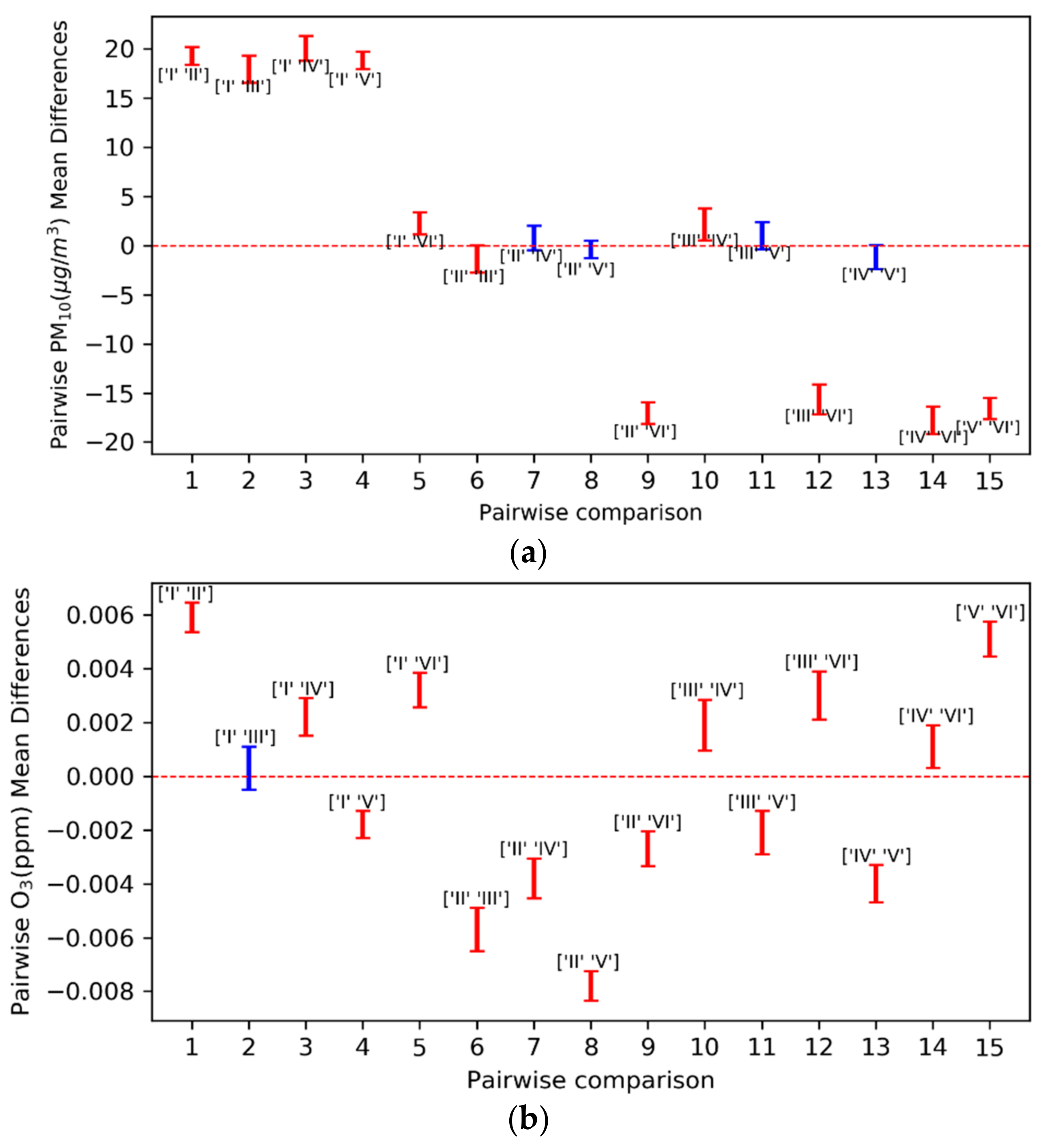
3.3. TSS Classification

Following the procedure explained in Section 2.3, and using a correlation coefficient of 0.6, over 100 groups (108) with different synoptic patterns were determined. Subsequently, the average sea level pressure maps of each of them were visually analyzed and reduced to expert judgment to only six groups; that is, six TSS. This reduction was possible because when examined individually, many of them referred to the same category. They were automatically classified as different, merely because the centers of action were displaced. The identified TSS in this study show a high level of agreement with the Isobaric Surface Configuration Types of Mosiño [18].

Table 2. Percentage of the six TSS from 1996 to 2016. USA: United States.

TSS	%
I   Thermal low over California *	23.85
II  Low pressure system over USA *	22.25
III Low pressure system over northeastern Mexico *	6.22
IV Extended trough on the east of the Sierra Madre Oriental *	8.55
V  High migratory pressures *	26.52
VI Convective-allowing situations *	11.61
Classified percentage **	79.15

* Relative to classified database, ** Relative to all dataset.

specifies the frequency of each identified TSS for the period 1996–2016.

Furthermore, Figure 9 shows the mean fields of sea level pressure for the six TSS identified in this research. TSS I (Figure 9a) consists of an area of low pressure over Baja California that is related to the heating of the Gulf of California and the dorsal of the Azores-Bermuda anticyclone extending over Central Mexico. The TSS II is a low-pressure system centered on the United States of America (USA). In this TSS, it may appear as a center of high pressure located in the eastern United States; see Figure 9b. With this pressure field, relatively high pressures can be found over central Mexico. TSS III in Figure 9c consists of an area of low pressure over northeastern Mexico. This type is recognized when the low center is close to the Gulf of Mexico or already on it, and it may be considered as a particular case of TSS II. The TSS IV stands for those configurations of the baric field that occurs when a trough extends over the east of the Sierra Madre Oriental to south of the Gulf of Mexico; see Figure 9d. This synoptic situation differs from TSS II regarding the intensity and extension of the trough. TSS V in Figure 9e shows the influence of high migratory pressures on the entire Mexican Republic. The center of the high-pressure system may be located in the central part of the USA, on the western Atlantic Ocean, or over the Gulf of Mexico. Lastly, the TSS VI is related to a weak subtropical anticyclonic influence, or to the existence of weak troughs or low-pressure systems over Mexico that favor convection, which is typical of the rainy season (Figure 9f).

Table 3. Means and standard deviations of O₃ and PM₁₀ hourly concentrations for each TSS.

TSS	PM10 (μg/m3)		O3 (ppm)
	Mean	Standard Deviation	Mean	Standard Deviation
TSS I	38.95	26.83	0.0252	0.0185
TSS II	58.44	35.69	0.0319	0.0247
TSS III	58.28	33.89	0.0289	0.0234
TSS IV	58.02	36.23	0.0246	0.0225
TSS V	58.72	36.13	0.0235	0.0208
TSS VI	42.94	28.70	0.0299	0.0216

shows the means and standard deviations of hourly concentrations of PM₁₀ and O₃ relative to each TSS. To determine whether there are differences between these averages, an ANOVA (one-way) analysis was performed. The ANOVA test has two critical assumptions that must be satisfied for the associated p-value to be valid: the observations within each group (TSS) must be normally distributed, and their standard deviations should be comparable (homoscedastic assumption). In this case, both conditions are satisfied. Also, one may say a priori that, for the PM₁₀ in TSS I and TSS VI, their means and standard deviations are already different from the rest of the TSS.

The statistical null hypothesis to test significant differences is that the averages of the hourly PM₁₀/O₃ concentrations are the same for the different TSS; the alternative hypothesis is that they are not all the same. If the p-value is less than or equal to the chosen significance level (0.05), the null hypothesis is rejected, and it is concluded that not all of the population means are equal. In both cases (i.e., PM₁₀ and O₃), their means were significantly heterogeneous: (one-way ANOVA, F_{5, 77511} = 1288.3, p < 0.001) for PM₁₀ concentrations and (one-way ANOVA, F_{5, 58314} = 420.4, p < 0.001) for O₃ levels. In both cases, F_{k−1, n−k} is the F-value of the test for k−1 and n−k degrees of freedom at 95% significance level, while p stands for the associated p-value from the F-distribution; see Table 1. Therefore, the null hypothesis is rejected, knowing that at least one pair of means has statistically significant differences.

The ANOVA analysis of the hourly concentrations of PM₁₀/O₃ was performed after subtracting its corresponding hourly means. Also, this analysis used observations that are valid from Monday to Thursday in the case of PM₁₀, and from Tuesday to Thursday for O₃ levels, in order to eliminate hourly and daily trends related to the anthropogenic activity. This way, only the local effects of the associated TSS on PM₁₀ and O₃ concentrations are considered. See Figure 3b and Figure 6b.

Afterward, Tukey’s test of multiple comparisons was applied to determine which pairs of PM₁₀ and ozone mean concentrations were statistically different. In this sense, Figure 10a,b show the results of the post-hoc analysis for PM₁₀ and O₃, respectively. These figures present the confidence intervals in error bars for all of the compared pairs of mean concentrations relative to each TSS. Whenever the error bars do not cross the y = 0 (discontinuous red) line, averages are said to be statistically different (red error bars). Otherwise, we cannot reject the null hypothesis that there are no differences (blue error bars) between each pair of elements.

For the PM₁₀ concentrations, Figure 10a shows (as expected) that TSS I and TSS VI are different from the rest. Among TSS II, III, IV, and V, there are no significant differences. Also, note that although TSS I and TSS VI are different from each other, they tend to be more similar, since its confidence interval is closest to y = 0. A visual comparison between Figure 9a,f could also support this finding, since their baric fields are alike. It can be seen in Table 3 that PM₁₀ averages for TSS I and TSS VI are the lowest of all six situations. This issue is easily explained: in both TSS, convergence will prevail in the GMA, which will favor the dispersion of the pollutants and also will increase the likelihood of precipitation on the region. It is evident that these two factors contribute to the cleaning of the atmosphere.

The spatial distributions of mean hourly concentrations of PM₁₀ in the GMA are shown in Figure 11a,b for TSS V and TSS I, respectively. In the GMA, the highest levels of PM₁₀ are found in TSS V (Figure 11a). During this TSS, thermal inversions are likely, which can occur on 78% of all days during the dry season [10]. During TSS I, the lowest levels of PM₁₀ are reported in the GMA, as shown in Figure 11b. Its spatial distribution, as in the case of TSS V, seems to be responding to the location of the main emitting sources of PM₁₀.

In the case of O₃ concentrations, in Figure 10b, all of the pairs of TSS results were statistically different except for the comparison between TSS I and TSS III. From Table 3, it can be seen that the ozone levels for TSS II, III, and VI are higher than those reported for TSS I, IV, and V. This result is somewhat surprising. One would expect low O₃ levels for TSS VI, because dispersion is more common during this TSS. Similarly, TSS V reported low ozone concentrations, even though it has been linked with thermal inversions. However, Comrie and Yarnal [46] found that ozone concentrations are sensitive to seasonality. Therefore, different behaviors in the O₃ levels for one TSS can be observed depending on whether it is the rainy or the dry season. Following this reasoning,

Table A3. Average hourly concentrations of O₃ (in ppm) for each TSS in the GMA for the rainy and dry seasons from 1996 to 2016.

TSS	Rainy Season	Dry Season
TSS I	0.0254	0.0244
TSS II	0.0386	0.0284
TSS III	0.0373	0.0280
TSS IV	0.0304	0.0226
TSS V	0.0273	0.0229
TSS VI	0.0295	0.0311

shows the hourly mean concentrations of ozone in the GMA for both seasons (dry and wet) within each TSS. It can be noted that TSS VI and TSS IV change their behavior with the season. While TSS VI presents higher values during the dry season, TSS IV shows higher concentrations in the dry season. However, TSS V reports low concentrations of O₃ in both periods. We did not relate these low values with an erroneous classification of the synoptic pattern, since this unusual behavior was only reported for ozone concentrations, and not for PM₁₀. Maximum values and the interannual variability of the O₃ means were analyzed (not shown here) to try to explain this unexpected feature. Those results did not allow us to justify the unexpected ozone concentrations during non-dispersive atmospheric conditions. These issues require further analysis; hence, it is recommended, as future work, to characterize the local circulations in the GMA for different TSS during the dry and wet seasons.

Furthermore, the spatial distribution of mean hourly concentrations of O₃ in the GMA are shown in Figure 11c,d for TSS II and TSS I, respectively. According to Figure 11c, during TSS II O₃, concentrations remain high all over the city with maximum values toward the north. This synoptic situation imposes weak horizontal pressure gradients with a clear sky and low wind speeds over the GMA. Tereshchenko and Filonov [9] studied some poor air quality episodes of high ozone levels in Guadalajara and linked them to a very similar TSS. In contrast, Figure 11d shows that the mean O₃ concentrations remain low in the city during TSS I.

4. Conclusions

To study the atmospheric pollution in the Guadalajara Metropolitan Area (GMA), the hourly concentrations of PM₁₀ and O₃ reported by eight monitoring stations located in the area were analyzed. Also, the six commonly found types of synoptic situations (TSS) during 1996–2016 were identified, and it was determined, statistically, which of them affect PM₁₀ and O₃ concentrations locally in the GMA.

Using hourly reported PM₁₀ and O₃ concentrations over the GMA, an exhaustive temporal and spatial characterization of these pollutants was introduced in the present research. At the time of writing, this characterization is the most updated and extensive one concerning the time range of the dataset analyzed for the GMA.

The temporal analysis of the PM₁₀ concentrations showed that their hourly levels in the GMA present two peaks. The first peak (82.68 μg/m³) was around 8 am local time, and a secondary one (74.54 μg/m³) was found close to 8 pm local time; both coincided with the busiest traffic schedules in the city. It was also found that the Mexican daily norm of 75.00 μg/m³ is frequently exceeded in the area of study, even reaching maximum daily values as high as 173.79 μg/m³. Additionally, weekly average concentrations of PM₁₀ were found to be higher during weekdays than on weekends due to traffic intensity.

Furthermore, the annual cycle of monthly concentrations of PM₁₀ is modulated by the behavior of precipitation in the area. The monthly average levels start rising in October, reaching their peak in December and maintaining high values until May, when the rainy season begins. Moreover, the interannual analysis of the PM₁₀ concentrations depicts a general trend of decrease in the annual mean levels of this pollutant for the period of study (1996–2016). On the other hand, the spatial distribution of the average concentrations in the GMA results in higher levels of PM₁₀ toward the south of Guadalajara (where more PM₁₀ emission sources are located), and lower concentrations northern of the city. This spatial pattern is because PM₁₀ particles are relatively large, so they tend to remain close to the emission sources. Due to their weight, they deposit before the wind can transport them.

The hourly concentrations of O₃ in the GMA reach their maximum (0.054 ppm) between 1–4 pm local time, in correspondence with the hours of maximum solar radiation. The Mexican norm for hourly ozone levels (0.095 ppm) is exceeded quite frequently, mainly in the mentioned time range. Regarding the eight hourly moving averages of O₃, the Mexican norm of 0.07 ppm is surpassed in all of the years. Additionally, the weekly analysis reported the presence of the weekend effect in the GMA. The latter means that the average concentrations of O₃ increase during the weekend, reaching its weekly maximum on Sundays (~0.0270 ppm). The comparison of the weekly values of O₃ and NO₂ indicates that the decrease in NO_x during the weekend keeps the formation of O₃ high.

Similar to what happens with PM₁₀, the monthly behavior of O₃ concentrations is modulated by the annual cycle of temperature and precipitation in the area of study. The levels begin to increase in January, reaching the maximum in May, from which they start to descend again to reach minimum values in December. The annual trend of O₃ shows a complex behavior. Therefore, it was divided into three main trend periods: (1996–1999), (2000–2011), and (2012–2016), which correspond, respectively, with a decrease, an increase, and a decrease again of the annual mean concentrations of O₃ in the GMA. There seems to be an inversely proportional relationship between the year-to-year ozone cycle and the solar cycle of sunspots. Further analysis of the implications of the 11-year sunspot cycle on the lower-troposphere ozone levels in the area of study is recommended. From the spatial analysis, it was noted that the highest concentrations of O₃ are reported north of the city.

The six TSS identified from the NARR data using the Lund technique were: TSS I “Thermal low over California”, TSS II “Low-pressure system over USA”, TSS III “Low-pressure system over northeastern Mexico”, TSS IV “Extended trough on the east of the Sierra Madre Oriental”, TSS V “High migratory pressures” and TSS VI “Convective-allowing situations”. This procedure allowed classifying 77.15% of the study period, with 20.85% remaining unclassified or within “Other situations”. It would be helpful to apply another TSS classification method in later works, such as orthogonal empirical functions (EOFs), to try reducing the percentage of days that were not classified in this research. Among all six of the TSS identified here, TSS V “High migratory pressures” was the most frequent, representing 26.52% of all classified cases.

The use of the ANOVA (one-way) technique allowed establishing that there are significant differences between the average concentrations of PM₁₀ and O₃ when grouped according to the TSS identified in this work. After doing the post-hoc analysis and making multiple comparisons between all of the possible pairs of means, it was determined that the PM₁₀ mean concentrations were different when comparing TSS VI and TSS I with the rest of the synoptic situations. Therefore, it can be said that during TSS VI and TSS I, PM₁₀ concentrations remained low on the GMA. Also, the PM₁₀ concentrations during TSS II, III, IV, and V were higher than those during TSS I and VI. Moreover, average concentrations of O₃ were higher under the influence of TSS II than with the rest of the TSS. The ozone levels observed during TSS IV and TSS V were lower than those measured under TSS II, III, and VI.

Ozone and PM₁₀ pollutants respond differently to the same types of synoptic situations. As a particulate matter, PM₁₀ is more dependent on wind, precipitation, and stability. Meanwhile, ozone (secondary pollutant) is more complicated and more affected by radiation. However, in both cases, their concentrations will depend on the local distribution of these meteorological variables.

All in all, it was found that the prevailing TSS locally influences the concentrations of PM₁₀ and O₃ in the GMA. Similarly, this methodology could be implemented in other places of interest to find statistically significant relationships between atmospheric pollutants levels and synoptic patterns. To complement what is analyzed in this paper, it is also recommended as future work to perform numerical simulations with the WRF/Chem model in order to study the local circulations imposed by each of the types of synoptic situations identified here, and their seasonal variability, in detail.

References

1. Penner, J.P.; Andreae, M.; Annegarn, H.; Barrie, L.; Feichter, J.; Hegg, D.; Achuthan, J.; Leaitch, R.; Murphy, D.; Nganga, J.; et al. Aerosols, their direct and indirect effects, in: Climate Change 2001: The Scientific Basis. In Contribution of Working Group I to the Third Assessment Report of the Intergovernmental Panel on Climate Change; Houghton, J.T., Ding, Y., Griggs, D.J., Noguer, M., Van der Linden, P.J., Dai, X., Maskell, K., Johnson, C.A., Eds.; Cambridge University Press: Cambridge, UK, 2001; pp. 289–348. [Google Scholar]
2. Pope, C.A., III; Dockery, D.W. Health effects of fine particulate air pollution: Lines that connect. J. Air Waste Manag. 2006, 56, 709–742. [Google Scholar] [CrossRef]
3. Zhang, J.; Mauzerall, D.L.; Zhu, T.; Liang, S.; Ezzati, M.; Remais, J.V. Environmental health in China: Progress towards clean air and safe water. Lancet 2010, 375, 1110–1119. [Google Scholar] [CrossRef]
4. PROAIRE (2011). Programa Para Mejorar la Calidad del Aire Jalisco 2011–2020. Inventario de Emisiones. Available online: http://www.semades.jalisco (accessed on 22 April 2018).
5. Kanda, I.; Basaldud, R.; Magaña, M.; Retama, A.; Kubo, R.; Wakamatsu, S. Comparison of ozone production regimes between two Mexican cities: Guadalajara and Mexico City. Atmosphere 2016, 7, 91. [Google Scholar] [CrossRef]
6. Benítez-García, S.E.; Kanda, I.; Wakamatsu, S.; Okazaki, Y.; Kawano, M. Analysis of criteria air pollutant trends in three Mexican metropolitan areas. Atmosphere 2014, 5, 806–829. [Google Scholar] [CrossRef]
7. Figueroa, A.; Davydova-Belitskaya, V.; Chávez, G.G.; Gallardo, T.P.; Orozco-Medina, M.G. PM10 y O3 como factores de riesgo de mortalidad por enfermedades cardiovasculares y neumonía en la Zona Metropolitana de Guadalajara, Jalisco, México. Ingeniería 2016, 20, 14–23. [Google Scholar]
8. Belitskaya, V.D.; Skiba, Y.N.; Martínez, A.; Bulgakov, S.N. Modelación matemática de los niveles de contaminación en la ciudad de Guadalajara, Jalisco, México. Parte II. Modelo numérico de transporte de contaminantes y su adjunto. Rev. Int. Contam. Ambient. 2001, 17, 97–107. [Google Scholar]
9. Tereshchenko, I.E.; Filonov, A.E. Acerca de las causas de las elevadas concentraciones de ozono en la atmósfera de la Zona Metropolitana de Guadalajara, en octubre de 1996. GEOS 1997, 17, 54–59. [Google Scholar]
10. Sánchez, H.U.R.; García, M.D.A.; Bejaran, R.; Guadalupe, M.E.G.; Vázquez, A.W.; Toledano, A.C.P.; de la Torre Villasenor, O. The spatial–temporal distribution of the atmospheric polluting agents during the period 2000–2005 in the Urban Area of Guadalajara, Jalisco, Mexico. J. Hazard. Mater. 2009, 165, 1128–1141. [Google Scholar] [CrossRef] [PubMed]
11. Stohl, A.; Hittenberger, M.; Wotawa, G. Validation of the Lagrangian particle dispersion model FLEXPART against large-scale tracer experiment data. Atmos. Environ. 1998, 32, 4245–4264. [Google Scholar] [CrossRef]
12. Varotsos, C.; Efstathiou, M.; Tzanis, C.; Deligiorgi, D. On the limits of the air pollution predictability: The case of the surface ozone at Athens, Greece. Environ. Sci. Pollut. Res. 2012, 19, 295–300. [Google Scholar] [CrossRef] [PubMed]
13. Bei, N.; Li, G.; Zavala, M.; Barrera, H.; Torres, R.; Grutter, M.; Gutiérrez, W.; García, M.; Ruiz-Suarez, L.G.; Ortinez, A.; et al. Meteorological overview and plume transport patterns during CalMex 2010. Atmos. Environ. 2013, 70, 477–489. [Google Scholar] [CrossRef]
14. Bei, N.; Li, G.; Huang, R.J.; Cao, J.; Meng, N.; Feng, T.; Molina, L.T. Typical synoptic situations and their impacts on the wintertime air pollution in the Guanzhong basin, China. Atmos. Chem. Phys. 2016, 16, 7373–7387. [Google Scholar] [CrossRef] [Green Version]
15. De Foy, B.; Varela, J.R.; Molina, L.T.; Molina, M.J. Rapid ventilation of the Mexico City basin and regional fate of the urban plume. Atmos. Chem. Phys. 2006, 6, 2321–2335. [Google Scholar] [CrossRef] [Green Version]
16. Notario, A.; Adame, J.A.; Bravo, I.; Cuevas, C.A.; Aranda, A.; Díaz-de-Mera, Y.; Rodríguez, A. Air pollution in the plateau of the Iberian Peninsula. Atmos. Res. 2014, 145, 92–104. [Google Scholar] [CrossRef] [Green Version]
17. Grundstrom, M.; Tang, L.; Hallquist, M.; Nguyen, H.; Chen, D.; Pleijel, H. Influence of atmospheric circulation patterns on urban air quality during the winter. Atmos. Pollut. Res. 2015, 6, 278–285. [Google Scholar] [CrossRef] [Green Version]
18. Mosiño, A.P. Una clasificación de las configuraciones del flujo aéreo en la República Mexicana. Rev. Ing. Hidraul. 1958, 12, 29–54. [Google Scholar]
19. INEGI (2011). Censo de Población Y Vivienda 2010. Tabulados del Cuestionario Básico. México. Available online: http://www3.inegi.org.mx/sistemas/TabuladosBasicos/Default.aspx?c=27302 (accessed on 25 April 2018).
20. Magaña, V.; Amador, J.A.; Medina, S. The midsummer drought over Mexico and Central America. J. Clim. 1999, 12, 1577–1588. [Google Scholar] [CrossRef]
21. Secretaría de Medio Ambiente y Desarrollo Territorial. Calidad del Aire AMG. Available online: http://siga.jalisco.gob.mx/aire2017/Descargas (accessed on 5 March 2018).
22. Secretaría de Medio Ambiente y Desarrollo Territorial. Sistema de Monitoreo Atmosférico de Jalisco. Available online: https://semadet.jalisco.gob.mx (accessed on 5 March 2018).
23. CLICOM. Available online: http://clicom-mex.cicese.mx (accessed on 21 November 2017).
24. CISL RDA: NCEP North American Regional Reanalysis (NARR). Available online: http://rda.ucar.edu/datasets/ds608.0/ (accessed on 25 May 2017).
25. Lund, I.A. Map-pattern classification by statistical methods. J. Appl. Meteorol. 1963, 2, 56–65. [Google Scholar] [CrossRef]
26. McDonald, J.H. Handbook of Biological Statistics; Sparky House Publishing: Baltimore, MD, USA, 2009; Volume 2, pp. 173–181. [Google Scholar]
27. Pandey, B.; Agrawal, M.; Singh, S. Assessment of air pollution around coal mining area: Emphasizing on spatial distributions, seasonal variations and heavy metals, using cluster and principal component analysis. Atmos. Pollut. Res. 2014, 5, 79–86. [Google Scholar] [CrossRef]
28. Fisher, R.A. Statistical Methods and Scientific Inference; Oliver & Boyd: Edinburgh, Scotland, UK, 1956. [Google Scholar]
29. Tukey, J.W. The philosophy of multiple comparisons. Stat. Sci. 1991, 6, 100–116. [Google Scholar] [CrossRef]
30. Stephens, S.; Madronich, S.; Wu, F.; Olson, J.B.; Ramos, R.; Retama, A.; Munoz, R. Weekly patterns of México City’s surface concentrations of CO, NOx, PM 10 and O3 during 1986–2007. Atmos. Chem. Phys. 2008, 8, 5313–5325. [Google Scholar] [CrossRef]
31. Gobierno del Estado de Jalisco. Reglamento de la Ley Estatal del Equilibrio Ecológico y la Protección al Ambiente en Materia de Prevención y Control de Emisiones por Fuentes Móviles; Gobierno del Estado de Jalisco: Guadalajara, Jalisco, México, 2012. [Google Scholar]
32. Nielsen-Gammon, J.W. The 2011 Texas drought. Texas Water J. 2012, 3, 59–95. [Google Scholar]
33. Elkus, B.; Wilson, K.R. Photochemical air pollution: Weekend-weekday differences. Atmos. Environ. 1977, 11, 509–515. [Google Scholar] [CrossRef]
34. Debaje, S.B.; Kakade, A.D. Weekend ozone effect over rural and urban site in India. Aerosol Air Qual. Res. 2006, 6, 322–333. [Google Scholar] [CrossRef]
35. Heuss, J.M.; Kahlbaum, D.F.; Wolff, G.T. Weekday/weekend ozone differences: What can we learn from them? Air Waste Manag. Assoc. 2003, 53, 772–788. [Google Scholar] [CrossRef]
36. Borrell P (2013). The Weekend Effect. Available online: http://www.rsc.org/chemistryworld/Issues/2003/May/weekend.asp (accessed on 5 October 2017).
37. Willett, H.C. The relationship of total atmospheric ozone to the sunspot cycle. J. Geophys. Res. 1962, 67, 661–670. [Google Scholar] [CrossRef] [Green Version]
38. Angell, J.K. On the relation between atmospheric ozone and sunspot number. J. Clim. 1989, 2, 1404–1416. [Google Scholar] [CrossRef]
39. Rafiq, L.; Tajbar, S.; Manzoor, S. Long term temporal trends and spatial distribution of total ozone over Pakistan. EJRS 2017, 20, 295–301. [Google Scholar] [CrossRef]
40. World Meteorological Organization (WMO). WMO Global Ozone Research and Monitoring Project; WMO: Geneva, Switzerland, 1985. [Google Scholar]
41. World Meteorological Organization (WMO). Scientific Assessment of Ozone Depletion: 1998 (Executive Summary); WMO: Geneva, Switzerland, 1999. [Google Scholar]
42. Coughlin, K.; Tung, K.K. Eleven-year solar cycle signal throughout the lower atmosphere. J. Geophys. Res. Atmos. 2004, 109. [Google Scholar] [CrossRef] [Green Version]
43. Labitzke, K.; Van Loon, H. Associations between the 11-year solar cycle, the QBO and the atmosphere. Part I: The troposphere and stratosphere in the northern hemisphere in winter. J. Atmos. Sol. Terr. Phys. 1988, 50, 197–206. [Google Scholar] [CrossRef]
44. Labitzke, K.; Van Loon, H. The signal of the 11-year sunspot cycle in the upper troposphere-lower stratosphere. Space Sci. Rev. 1997, 80, 393–410. [Google Scholar] [CrossRef]
45. Chandra, S.; Ziemke, J.R.; Stewart, R.W. An 11-year solar cycle in tropospheric ozone from TOMS measurements. Geophys. Res. Lett. 1999, 26, 185–188. [Google Scholar] [CrossRef] [Green Version]
46. Comrie, A.C.; Yarnal, B. Relationships between synoptic-scale atmospheric circulation and ozone concentrations in metropolitan Pittsburgh, Pennsylvania. Atmos. Environ. Part B Urban 1992, 26, 301–312. [Google Scholar] [CrossRef]
Figure 1. Area of study. (a) Region where the types of synoptic situations (TSS) were analyzed. (b) A zoom of the Guadalajara Metropolitan Area (GMA) is enclosed in (a) with a red square. The red circles filled in black show the location of the measurement stations.
Atmosphere 09 00243 g001
Figure 2. Mean meteorological variables in the GMA for the period 1996–2016. (a) Average annual cycle of precipitation and temperature. (b) Diurnal cycle of temperature and mean wind speed. Wind direction frequency for the rainy (c) and the dry seasons (d).
Atmosphere 09 00243 g002
Figure 3. Hourly box-plot (a), weekly bar chart (b), and daily time series (c) of mean concentrations of PM10 (in μg/m3) using the data reported by the eight measurement stations from 1996 to 2016 in the GMA. In (a), the bottom and top of boxes represent the 25th and 75th percentiles, respectively, the ends of whiskers represent the sample minimum and maximum, while the horizontal red line near the middle of boxes is the 50th percentile. Plus-sign marks represent extreme values.
Atmosphere 09 00243 g003
Figure 4. Monthly bar chart (a) and yearly (b) average concentrations of PM10 (in μg/m3) using the data reported by the eight measurement stations from 1996 to 2016 in the GMA. Discontinuous green line depicts the general trend, and the red line highlights the Mexican norm.
Atmosphere 09 00243 g004
Figure 5. Spatial behavior of the mean PM10 (in μg/m3) concentrations in the GMA using the objective mapping interpolation method. The white lines represent the interpolation errors.
Atmosphere 09 00243 g005
Figure 6. Hourly box-plot (a), weekly bar chart (b), and (c) annual maxima of the eight-hour moving average of O3 levels (in ppm) from 1996 to 2016 in the GMA. Blue bars in (b) represent mean concentrations of NO2 (in ppm). Discontinuous red and blue lines highlight the Mexican norm and the World Health Organization (WHO) recommendation, respectively. In (a), the bottom and top of the boxes represent the 25th and 75th percentiles, respectively, the ends of whiskers represent the sample minimum and maximum, while the horizontal red line near the middle of boxes is the 50th percentile. Plus-sign marks represent extreme values.
Atmosphere 09 00243 g006
Figure 7. Monthly bar chart (a) and yearly (b) average concentrations of O3 (in ppm) using the data reported by the eight measurement stations from 1996 to 2016 in the GMA. The discontinuous green lines depicts the time interval trends.
Atmosphere 09 00243 g007
Figure 8. Spatial behavior of the mean O3 (in ppm) concentrations in the GMA using the objective mapping interpolation method. The white lines represent the interpolation errors.
Atmosphere 09 00243 g008
Figure 9. Mean sea level pressure fields (in hPa) for the six TSS identified in this research: (a) TSS I, (b) TSS II, (c) TSS III, (d) TSS IV, (e) TSS V, and (f) TSS VI.
Atmosphere 09 00243 g009
Figure 10. Multiple comparisons of all concentration pairs for (a) PM10 (in μg/m3) and (b) O3 (in ppm) relative to each TSS. The red error bars stand for statistically different averages, and the blue ones represent the opposite.
Atmosphere 09 00243 g010
Figure 11. Spatial distribution of the mean PM10 (in μg/m3) concentrations for (a) TSS V and (b) TSS I; and spatial behavior of the mean O3 (in ppm) concentrations for (c) TSS II and (d) TSS I in the GMA. The white lines represent the interpolation errors.
Atmosphere 09 00243 g011