Avoiding Extremes: Benefits of Staying below +1.5 °C Compared to +2.0 °C and +3.0 °C Global Warming

Abstract

The need to restrict global mean temperature to avoid irreversible climate change is supported by scientific evidence. The need became political practice at the Conference of the Parties in 2015, where the participants decided to limit global warming to not more than +2.0 °C compared to pre-industrial times and to rather aim for a limit of +1.5 °C global warming. Nevertheless, a clear picture of what European climate would look like under +1.5 °C, +2.0 °C and +3.0 °C global warming level (GWL) is still missing. In this study, we will fill this gap by assessing selected climate indices related to temperature and precipitation extremes, based on state of the art regional climate information for Europe taken from the European branch of the World Climate Research Program Coordinated Regional Downscaling Experiment (EURO-CORDEX) ensemble. To assess the impact of these indices under climate change, we investigate the spatial extent of the area of the climate change signal in relation to the affected population. This allows us to demonstrate which climate extremes could be avoided when global warming is kept well below +2.0 °C or even +1.5 °C compared to higher GWLs. The European north–south gradient of tropical nights and hot days is projected to be intensified with an increasing global warming level. For precipitation-related indices, an overall increase in precipitation extremes is simulated, especially under +3.0 °C GWL, for mid- and northern Europe, whereas an increase in dry days is projected for many regions in southern Europe. The benefit of staying below +1.5 °C GWL compared to +2.0 °C GWL is the avoidance of an additional increase in tropical nights and hot days parallel to an increase in dry days in parts of southern Europe as well as an increase in heavy precipitation in parts of Scandinavia. Compared to +3.0 °C GWL, the benefit of staying at +1.5 °C GWL is to avoid a substantial increase (i.e., an increase of more than five dry days and ten tropical nights) in dry days and tropical nights in southern European regions, while, in several European regions and especially in northern Europe, a substantial increase (i.e., more than two heavy precipitation days) in heavy precipitation days could be avoided. This study shows that a statistically significant change in the investigated climate indices can be avoided under +1.5 °C GWL compared to the investigated higher GWLs +2.0 °C and +3.0 °C for the majority of the population in almost all regions. Future studies will investigate compound events where the severity of single extreme events is intensified.

1. Introduction

The Conference of the Parties of the United Nations Framework Convention on Climate Change (UNFCCC) in December 2015 surprised many people by pledging not just to keep mean global warming “well below 2 degrees Celsius,” but also to pursue efforts to limit warming to +1.5 °C global warming above pre-industrial levels. This raised important questions for researchers: what is the difference between +2.0 °C and +1.5 °C mean global warming? To which climate change and related extremes do we have to adapt under +2.0 °C and +1.5 °C global warming? How many people will be exposed to extreme climate change if we do not keep to the +1.5 °C global warming threshold? This difference is important for decisions on whether to increase the ambition of climate change mitigation efforts to stabilize temperatures at +1.5 °C rather than +2.0 °C above pre-industrial levels [1].

There is still no clear picture of what a +1.5 °C or +2.0 °C world or above might look like and which population will be affected most by climate changes under the different thresholds. A number of studies have begun to assess climate change at +2.0 °C mean global warming in Europe (e.g., [2]) and beyond (e.g., [3]). However, the distinction between the increments of global mean temperature increase between +1.5 °C up to +3.0 °C or above) has received limited scientific attention, especially in terms of regional and local impacts [4].

Different methods have been proposed to assess the impacts of the specific warming levels [4]. Studies using increments of global mean temperature increase vary in their choice of baseline [5]. Most of the studies assessing climate change impacts in Europe focus at fixed time periods, for example, mid- or end century [6,7]. However, to set targets for climate change mitigation at levels of global mean temperature change relative to pre-industrial levels is a more appealing and intuitive way to analyze the regional impacts of a global warming. General circulation models (GCMs) project different global mean temperatures at a fixed time period due to their different climate sensitivities. The approach used in this study avoids the uncertainty of different climate sensitivities by looking at fixed GWLs. At a fixed GWL, the uncertainty due to the different climate sensitivities of the GCMs does not just disappear but lies in the differences of the time periods in which the fixed GWL is reached. However, this uncertainty in time periods of GWLs is of minor importance in this study, as it focuses only on climatic conditions under different GWLs, which depend to a lesser extent on when exactly a certain GWL is reached. An additional reason to use this approach is that assessments of climate change impacts at GWLs are frequently requested by stakeholders and decision makers.

To support decision-making, we investigate here the changes of indices related to climate extremes at the levels of +1.5 °C, +2.0 °C and +3.0 °C global warming in comparison to pre-industrial levels. To assess the strength of the impact of these changes, we investigate the spatial extent of the area of significant climate change signals as well as the population affected by these changes. This allows us to demonstrate which climate extremes could be avoided when keeping the global warming well below +2.0 °C or even +1.5 °C.

A key issue in setting policy targets is that it encourages ambitious decision makers to meet the targets. In addition, comparing targets in global warming temperatures clearly point out the different consequences for the regional climate and a specific sector. A way to examine the benefits for each sector when keeping global warming below a specific target is to analyse climate extreme indices. Such climate extreme indices can be used to describe the state and the changes in the climate system. Climate extreme indices are derived from daily temperature and precipitation as defined, e.g., by the Expert Team on Climate Change Detection and Indices (ETCCDI, [8]).

For strategic approaches to mitigation and adaptation, characterizing and quantifying uncertainty in climate change projections is of fundamental importance. Uncertainties due to natural variability and the emissions sensitivity of climate models can be accounted for by using a combination of climate model simulations [9]. Here, the study is based on an ensemble of high-resolution regional climate simulations at 0.11° × 0.11° (about 12.5 km × 12.5 km) gridbox size provided by the EURO-CORDEX (coordinated downscaling experiment—European domain, [7]) community. The robustness of the results is assessed by statistical testing.

This study contributes to identifying which regions in Europe may be exposed to the strongest impacts of climate change under consideration of the affected population depending on the ambition of climate change mitigation efforts to stabilize global mean temperatures at certain degrees Celsius above pre-industrial levels. The study supports decision-making towards ambitious climate change mitigation efforts to stabilize temperatures at +1.5 °C mean global warming by pointing out what climate extremes could be avoided in which regions. This is done by a quantitative comparison of expected changes in key climate indices related to temperature and precipitation extremes and the affected population in different regions in Europe under three warming levels: +1.5 °C, +2.0 °C and +3.0 °C.

2. Data and Methods

Selected regions represent a profile of Europe’s climate, ranging from the Iberian Peninsula to France and Mid-Europe and to Scandinavia. In order to investigate possible changes in extremes in Europe, climate indices based on temperature and precipitation are analysed over representative PRUDENCE regions [10]. For this study, out of a larger group of indices, we selected five temperature and precipitation related climate indices showing statistically significant changes (refer to the paragraph “Statistical test”) under climate change conditions over larger inhabited land areas of Europe, which we identified in a preparatory work. Our selection was guided by the aim to cover temperature extremes during day and night-time as well as drought conditions and heavy precipitation. The indices used in this study are listed in

Table 1. Table of indices and their definition according to or adapted from the Expert Team on Climate Change Detection and Indices (ETCCDI) [11,12].

Description	Abbreviation	Definition	Unit	Reference
Hot days	Hot days	Number of days with a maximum temperature Tmax > 30 °C	days/year	Adapted from ETCCDI
Tropical nights	Tnights	Number of nights with minimum temperature Tmin > 20 °C	days/year	ETCCDI
Number of dry days	Rlt1mm	Number of days with precipitation pr < 1 mm	days/year	Adapted from ETCCDI
Number of heavy precipitation days	R10mm	Number of days with precipitation pr > 10 mm	days/year	ETCCDI
99th percentile of precipitation	R99p	99th percentile of wet days per year (days with precipitation r ≥ 1 mm)	mm/day	ETCCDI

. Most of the indices could be taken directly from ETCCDI indices [11,12] which are designed for global assessments. Instead of the ETCCDI index summer days (SU), defined as the number of days with a maximum temperature above 25 °C, we are using hot days, which are more appropriate for assessing extremes in Europe (definition see Table 1). In addition, instead of the ETCCDI index wet days (R1mm), we use the number of dry days (Rlt1mm) using the same threshold, as the number of dry days are more relevant for adaptation in Europe (definition see Table 1).

2.1. Climate Data

Climate information is based on regional climate model (RCM) simulation data of the EURO-CORDEX ensemble at 0.11° × 0.11° (about 12.5 km × 12.5 km) gridbox size [7], which has been proven to simulate the European climate in various studies (e.g., [13,14]). In this study, a subset of the EURO-CORDEX ensemble (see

Table 2. Regional climate model (RCM)-general circulation model (GCM) combinations (16 in total) of the simulations used in this study, and the 30-year period centers under which the GCM shows a global warming level (GWL) of +1.5 °C, +2.0 °C and +3.0 °C. RCP: representative concentration pathway.

GCM, RCP, Realization	RCMs	+1.5 °C Period	+2.0 °C Period	+3.0 °C Period
CNRM-CM5, RCP8.5, r1i1p1	CCLM, RCA4	2015–2044	2030–2059	2053–2082
EC-EARTH, RCP8.5, r12i1p1	CCLM, RACMO, RCA4	2012–2041	2027–2056	2052–2081
IPSL-CM5A, RCP8.5, r1i1p1	WRF, RCA4	2008–2037	2021–2050	2040–2069
HadGEM2, RCP4.5, r1i1p1	CCLM, RACMO, RCA4	2007–2036	2023–2052	2055–2084
HadGEM2, RCP8.5, r1i1p1	CCLM, RACMO, RCA4	2006–2035	2016–2045	2037–2066
MPI-ESM, RCP8.5, r1i1p1	CCLM, REMO2009, RCA4	2014–2043	2030–2059	2053–2082

) is used, considering only those GCM-RCM combinations, for which climate information for global warming levels of +1.5 °C, +2.0 °C and +3.0 °C are available. This assures comparability between the results under different global warming levels, but excludes, e.g., all simulations driven by the representative concentration pathway (RCP) 2.6 [15] scenario as they do not reach +3.0 °C global warming.

2.2. Global Climate Change Signal Selection Method

This study focuses on climate change information under the different global warming levels (GWL) +1.5 °C, +2.0 °C and +3.0 °C with respect to pre-industrial (1881–1910) climate conditions. While there are various approaches to identify regional climate signals associated with global temperature limits [4], we have chosen the time sampling approach following the impact2c project (www.impact2c.eu): In the first step, and for each of the GCMs, the 30-year periods are identified in which the GWLs are reached for the first time in their mean value over this period. In the second step, the downscaled regional climate information is taken from the 30-year periods of the driving GCMs and the respective GWLs [2]. Following the approach of [2], the global warming between the pre-industrial reference period (1881–1910) and the present-day reference period (1971–2000) is calculated based on observations as +0.46 °C. The future 30-year periods for the remaining global warming for each of the GWLs (e.g., +1.54 °C for +2 °C GWL) are calculated based on climate conditions projected by the individual GCMs. The GCMs used in this study are HadGEM2 [16], EC-EARTH [17], CNRM-CM5 [18], IPSL-CM5A [19], MPI-ESM [20,21,22]. The RCMs used in this study are evaluated and referenced in [13].

A list of RCM-GCM combinations together with the future 30-year periods of the GWLs +1.5 °C, +2.0 °C and +3.0 °C can be found in Table 2.

By applying the method of using a fixed GWL, the spread of GCM climate change signals is reduced compared to a reference time period with a fixed time period in the future. Nevertheless, by fixing the GWL in the GCM, the paths of how to reach them, including the speed in which the climate change occurs, differs for each GCM-RCP combination because of different climate sensitivities in the GCMs. The time that is left until a distinct GWL is reached is essential for the adaptation of natural and human systems, though it is not part of this study. In addition, a higher RCP can lead to a faster transient global warming during the identified GWL period. This has to be kept in mind when interpreting the results of this study.

2.3. Regional Climate Change Signals at Different GWLs

The climate change signals and their significance information are calculated based on the EURO-CORDEX ensemble data for each GWL. While the GWLs are calculated based on the pre-industrial reference period 1881–1910, RCM simulations only start after 1950. Therefore, the climate change signals of the RCM simulations can only be computed with respect to the present-day reference period 1971–2000. The period from pre-industrial times to the present-day reference period already includes a global climate change signal of +0.46 °C (see, e.g., [2]). This means that climate change signals of the RCM simulations under +2.0 °C GWL correspond to a response to +1.54 °C global warming. This has to be kept in mind when interpreting the results.

2.4. Population Data

In order to investigate the potential impact of climate change on humans under different GWLs, we use fixed population density data projected to the year 2015 [23]. It is remapped to the EURO-CORDEX model domain and used to calculate the absolute number of inhabitants per gridbox. This information is further used to investigate the potentially affected population by significant climate change under the different GWLs.

2.5. Statistical Test

The two-sided Mann–Whitney-U test [24] is applied for each gridbox and each simulation. The reference period is compared to the future climate period for each of the three GWLs and is counted as significant on a 90% confidence level. If more than 66% of the simulations show a significant climate change signal, the climate change signal of the ensemble is defined as significant. The choice of the confidence level and the threshold for the simulations showing a significant climate change signal is guided by [25]. In this study, we chose a slightly higher confidence of level of 90% than the 85% used in [25].

2.6. Calculated Values for the PRUDENCE Regions

First, the climate change signal and its significance are calculated for each climate index. Second, spatial mean values are calculated for those areas in each PRUDENCE region in which the climate index reveals a significant climate change signal. As an indication for the spread of the climate change signal, the area mean is calculated for the minimum, median and maximum of the ensemble.

In addition, the climate change signal is combined with the population density data set. For each PRUDENCE region and climate index, the significant areas of climate change are overlaid with the population density per grid box. By doing so, the fraction of affected population can be determined. Population living in densely populated areas (more than 1000 inhabitants per km²) might be affected more severely, and this is listed separately. Finally, the fraction of the affected land-surface area per PRUDENCE region gives an indication of the importance of the change of each climate index. Absolute values of population, population living in densely populated areas and the total land surface area of the PRUDENCE regions are listed in

Table 3. Absolute values of population, population living in densely populated areas (areas with more than 1000 inhabitants per km²) and the total land surface are shown as used within this study. Population data is take from [23].

PRUDENCE Region	Population (Million Inhabitants)	Population in Densely Populated Areas (Million Inhabitants)	Total Land-Surface Area (in 1000 km2)
British Isles	68.8	53.0	380.6
Iberian Peninsula	66.8	30.9	679.1
France	40.3	17.1	364.1
Mid-Europe	143.2	61.5	629.2
Scandinavia	36.0	9.7	1488.4
Alps	50.4	17.5	318.9
Mediterranean	83.8	28.4	696.6
Eastern Europe	116.0	36.7	1215.3

as a reference.

3. Results

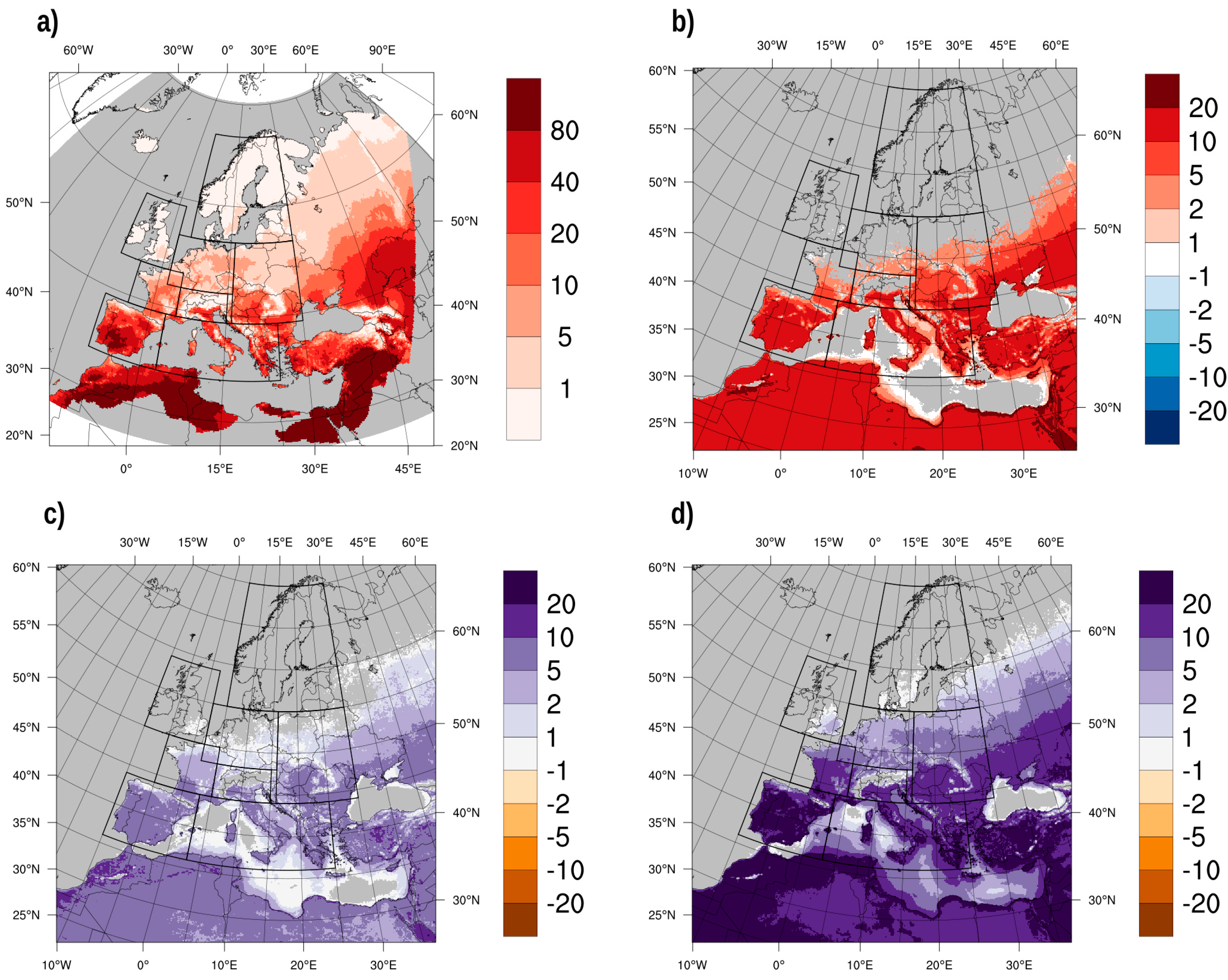
The results of this study are presented in two ways. The spatial extent of each climate index (see Table 1) is shown in Figure 1, Figure 2, Figure 3, Figure 4 and Figure 5, presented by the present-day climate conditions using the European observation E-OBS gridded dataset [26] and by its climate change signal at +1.5 °C GWL. This is accompanied by the difference between the climate change signals for a +2.0 °C GWL and a +3.0 °C GWL in comparison to the climate change signal under +1.5 °C GWL, respectively. The latter can be interpreted as the avoided change of the respective climate index if the GWL does not exceed +1.5 °C. Climate change signals are shown for areas where a significant climate change signal is present. Differences of climate change signals are shown for areas in which the climate index is significant in the ensemble at the higher GWL.

The spatial mean of the change of the five climate indices (see Table 1) at +1.5 °C, +2.0 °C and +3.0 °C GWL can be found in

Table 4. Indices (refer to Table 1) and their parameters are shown for PRUDENCE regions (refer to Table 3) and GWLs +1.5 °C, +2.0 °C and 3.0 °C. The parameter E-OBS indicates the reference value as represented by the E-OBS European observation data for each climate index under the present-day climate, averaged over the area in which significant climate change is projected under the respective GWL for the respective index. The parameter CCS (ens min/max) indicates the mean climate change signal and the ensemble minimum and maximum, averaged over the area in which significant climate change is projected under the respective GWL for the respective index. The parameters pop/pop densly indicate the percentage of the population and of the population living in densely populated areas, respectively, which is affected by a significant change in the respective climate index. Similarly, the parameter area indicates the percentage of the area that is affected by a significant change in the respective climate index. For more details refer to the text.

Index	Parameter	British Isles			Iberian Peninsula			France
		+1.5 °C	+2.0 °C	+3.0 °C	+1.5 °C	+2.0 °C	+3.0 °C	+1.5 °C	+2.0 °C	+3.0 °C
Hot days	E-OBS in CCS area	0.4	1.0	0.7	41.5	40.5	40.2	10.1	8.3	8.2
	CCS (ens min/max)	0.5 (−0.3/3.8)	0.8 (−0.1/6.9)	1.7 (0.2/10.1)	11.2 (4.7/18.1)	15.8 (7.0/26.1)	25.8 (12.5/39.8)	4.1 (0.5/14.7)	6.3 (1.7/22.3)	13.4 (3.6/31.3)
	pop/pop densly in %	6.5/7.8	32.0/35.2	78.1/82.0	91.4/88.7	99.1/100.0	99.9/100.0	33.8/17.2	97.7/100.0	99.7/100.0
	area in %	0.7	10.7	32.0	93.5	96.9	98.8	47.9	94.5	98.0
Tnights	E-OBS in CCS area	0.0	0.0	0.0	6.9	6.3	5.9	0.4	0.4	0.3
	CCS (ens min/max)	0.7 (0.0/12.4)	1.1 (−0.1/15.6)	2.5 (0.0/19.2)	10.9 (4.9/22.3)	16.3 (6.9/31.9)	29.6 (14.2/48.7)	3.3 (0.3/18.4)	5.8 (0.8/25.0)	14.2 (3.4/40.3)
	pop/pop densly in %	0.3/0.0	9.9/10.4	71.5/75.5	96.1/98.5	98.8/100.0	99.7/100.0	92.0/100.0	97.7/100.0	99.9/100.0
	area in %	0.9	4.6	32.7	84.1	92.0	97.3	81.5	93.0	99.1
Rlt1mm	E-OBS in CCS area			173.5	315.9	294.3	280.1			230.4
	CCS (ens min/max)			9.9 (−5.0/19.6)	6.8 (2.3/12.7)	8.3 (3.1/19.0)	13.1 (4.4/22.6)			9.4 (−7.3/18.3)
	pop/pop densly in %			2.1/0.5	1.2/0.0	42.6/37.3	88.0/82.4			14.9/9.3
	area in %			14.0	3.3	51.5	97.1			24.2
R10mm	E-OBS in CCS area	17.8	23.6	17.8		16.2	20.7	16.5		15.6
	CCS (ens min/max)	2.7 (−0.5/5.4)	3.0 (0.6/6.1)	3.6 (1.2/7.5)		−3.1 (−7.8/−0.2)	−4.4 (−9.3/−0.6)	2.7 (−2.6/6.2)		3.4 (1.0/8.2)
	pop/pop densly in %	0.7/0.6	3.3/3.4	61.7/62.9		0.8/0.0	21.6/18.2	3.3/4.8		34.6/59.0
	area in %	1.0	3.3	40.1		0.9	23.2	2.4		15.6
R99p	E-OBS in CCS area		30.9	23.7			19.7		22.0	19.5
	CCS (ens min/max)		2.6 (−0.6/5.5)	3.3 (0.5/6.6)			7.8 (0.9/17.8)		3.1 (−1.5/7.7)	4.0 (0.1/10.2)
	pop/pop densly in %		0.3/0.0	22.8/20.7			0.2/0.0		0.6/0.0	25.4/10.4
	area in %		2.5	42.1			1.5		0.9	33.4
Index	Parameter	Mid-Europe			Scandinavia			Alps
		+1.5 °C	+2.0 °C	+3.0 °C	+1.5 °C	+2.0 °C	+3.0 °C	+1.5 °C	+2.0 °C	+3.0 °C
Hot days	E-OBS in CCS area	4.6	5.2	4.6		1.1	0.9	12.2	10.2	8.8
	CCS (ens min/max)	2.6 (0.3/7.1)	3.4 (1.1/13.7)	6.6 (2.6/19.3)		1.0 (−0.1/6.5)	1.7 (0.1/8.1)	6.1 (1.1/13.7)	7.8 (1.8/23.0)	13.5 (4.6/31.2)
	pop/pop densly in %	19.1/13.3	63.7/63.6	99.7/99.7		0.5/0.0	42.6/54.2	81.7/90.7	91.3/97.6	95.6/98.6
	area in %	23.7	63.8	97.5		0.6	21.9	52.6	66.8	77.3
Tnights	E-OBS in CCS area	0.1	0.1	0.1		0.0	0.0	5.9	4.7	3.6
	CCS (ens min/max)	1.2 (0.0/8.5)	1.4 (0.1/10.6)	3.8 (0.4/17.0)		1.4 (0.0/11.0)	2.0 (0.1/16.3)	10.3 (2.6/19.5)	13.0 (3.5/28.2)	19.3 (6.9/37.5)
	pop/pop densly in %	34.7/44.3	78.9/87.4	99.9/100.0		6.1/13.0	32.1/51.3	69.1/80.1	80.4/90.9	91.5/96.3
	area in %	27.3	66.7	99.5		2.8	17.6	43.7	53.2	67.4
Rlt1mm	E-OBS in CCS area					251.3	246.8			257.5
	CCS (ens min/max)					−8.4 (−15.6/4.7)	−10.0 (−18.6/5.1)			10.1 (−1.1/19.5)
	pop/pop densly in %					0.2/0.0	2.4/0.0			2.0/0.9
	area in %					2.5	9.2			7.0
R10mm	E-OBS in CCS area	13.6	12.6	15.4	10.9	12.4	14.1			31.0
	CCS (ens min/max)	3.1 (0.1/6.3)	2.9 (0.3/7.0)	3.8 (1.1/8.5)	2.6 (0.3/5.1)	3.3 (0.8/6.2)	4.8 (1.6/8.8)		3.5 (−1.1/8.7)	4.0 (−0.7/10.6)
	pop/pop densly in %	3.2/3.7	17.6/19.9	88.0/90.7	26.4/33.0	65.3/64.9	93.8/100.0		0.9/0.0	6.1/2.4
	area in %	5.1	22.5	84.8	27.8	74.1	93.5		1.4	6.8
R99p	E-OBS in CCS area			18.4	15.7	15.7	17.3		39.4	33.7
	CCS (ens min/max)			3.7 (0.0/8.4)	2.9 (−0.7/5.7)	3.0 (−0.0/6.0)	3.7 (0.6/7.4)		5.9 (−0.9/13.4)	7.5 (0.9/17.9)
	pop/pop densly in %			37.7/38.3	0.5/0.0	9.3/7.8	61.2/55.3		0.1/0.0	24.6/25.7
	area in %			34.1	0.9	14.3	69.9		0.7	20.5
Index	Parameter	Mediterranean			Eastern Europe
		+1.5 °C	+2.0 °C	+3.0 °C	+1.5 °C		+2.0 °C		+3.0 °C
Hot days	E-OBS in CCS area	27.3	27.0	26.8	11.1		9.5		8.4
	CCS (ens min/max)	7.5 (1.9/18.2)	9.6 (2.7/25.4)	17.6 (5.2/37.2)	7.0 (2.6/14.5)		9.4 (3.4/16.8)		14.1 (7.4/24.9)
	pop/pop densly in %	99.3/100.0	99.7/100.0	99.9/100.0	68.1/60.1		85.9/79.7		99.9/100.0
	area in %	97.5	99.1	99.7	64.6		82.9		99.6
Tnights	E-OBS in CCS area	11.8	11.2	10.6	1.1		0.8		0.7
	CCS (ens min/max)	17.4 (11.2/25.8)	24.3 (15.8/37.3)	38.1 (26.6/54.4)	4.9 (0.9/15.3)		6.1 (1.1/18.5)		11.1 (3.1/29.5)
	pop/pop densly in %	95.5/98.4	97.7/99.5	99.2/100.0	71.8/70.5		94.5/98.2		99.2/100.0
	area in %	87.6	92.4	96.9	64.9		89.7		97.7
Rlt1mm	E-OBS in CCS area		287.1	281.0					242.5
	CCS (ens min/max)		7.4 (1.2/18.4)	9.7 (−1.1/19.5)					8.4 (−1.1/18.4)
	pop/pop densly in %		9.3/16.1	61.5/62.1					0.2/0.0
	area in %		5.5	65.2					0.7
R10mm	E-OBS in CCS area			20.8	11.8		11.7		12.5
	CCS (ens min/max)			−4.2 (−10.0/4.3)	2.6 (0.4/5.5)		2.6 (0.6/5.9)		3.4 (1.3/8.1)
	pop/pop densly in %			12.3/11.7	2.9/4.9		32.9/40.5		73.7/79.0
	area in %			10.0	3.0		29.0		68.3
R99p	E-OBS in CCS area		43.1	23.7			18.6		18.0
	CCS (ens min/max)		8.1 (−0.0/22.0)	8.6 (0.8/21.6)			3.9 (−0.5/8.3)		4.9 (0.3/9.8)
	pop/pop densly in %		1.4/3.1	13.9/16.1			1.5/1.6		33.8/32.5
	area in %		0.6	12.4			1.4		34.0

. The incremental climate changes are listed for each PRUDENCE region. The ensemble mean of each climate change signal is accompanied by its ensemble minimum and maximum. In addition, for each climate index, the reference value derived from the E-OBS observation data in the period from 1971–2000 is given. To assess the strength of the impact of the changes, the spatial extent of the climate change signal per region is presented. The share of affected population for each climate index is given for the entire population and for the population living in densely populated areas.

The analysis is guided by investigating the changes along a transect over the European continent stretching from the Iberian peninsula through France and Mid-Europe to Scandinavia.

3.1. Hot Days

Present day conditions represented by E-OBS show a north–south gradient for hot days with values of more than 80 days/year over parts of the central Iberian Peninsula and between 20 and 40 days/year in many parts of the Mediterranean region to zero days in most parts of Scandinavia (refer to Figure 1a).

Under the +1.5 °C GWL, a substantial increase in the number of hot days is projected for southern and south-west Europe as well as for parts in central and eastern Europe (refer to Figure 1b). Those regions with increasing number of hot days extend northwards under +2.0 °C GWL and even further under +3.0 °C GWL as shown by the increase in hot days in areas where no hot days are projected to increase under +1.5 °C GWL (see Figure 1c,d for +2.0 °C GWL and +3.0 °C GWL, respectively).

The strongest changes are simulated over the Iberian Peninsula, with 11.2 (ensemble spread: 4.7 to 18.1) more hot days per year under +1.5 °C global warming for almost the whole area and 91% of the total population—89% of the population living in densely populated areas—affected by significant increases in the number of hot days. Under +2.0 °C and +3.0 °C global warming, the whole population is affected by an increase in hot days of 15.8 (7.0 to 26.1) and 25.8 (12.5 to 39.8), respectively.

In Mid-Europe, under a +1.5 °C GWL, 19% of the population are affected by an increase of 2.6 hot days (0.3 to 7.1). Under the +2.0 °C global warming scenario, 64% of the total population are affected by 3.4 (1.1 to 13.7) more hot days per year; under +3.0 °C GWL, 99.7% of the population of Mid-Europe is exposed to an increase in the number of hot days, with 6.6 more days per year with an ensemble spread between 2.6 to 19.3.

In Scandinavia, in contrast, no region and no population is affected by an increase in the number of hot days under +1.5 °C GWL—and also under +2.0 °C GWL. Only under the +3.0 °C GWL would more than 40% of the population be exposed to an increase in the number of hot days of 1.7 days per year with an ensemble spread of 0.1 to 8.1.

Over the Iberian Peninsula and the Mediterranean, almost the whole population would be exposed to an increase in hot days, but under the +3.0 °C GWL, the increase is more than double as in the case of the +1.5 °C GWL. In most of the other regions, far fewer people would be exposed to more hot days, especially under +1.5 °C and +2.0 °C GWL. For all values, a large ensemble spread compared to the mean results can be observed.

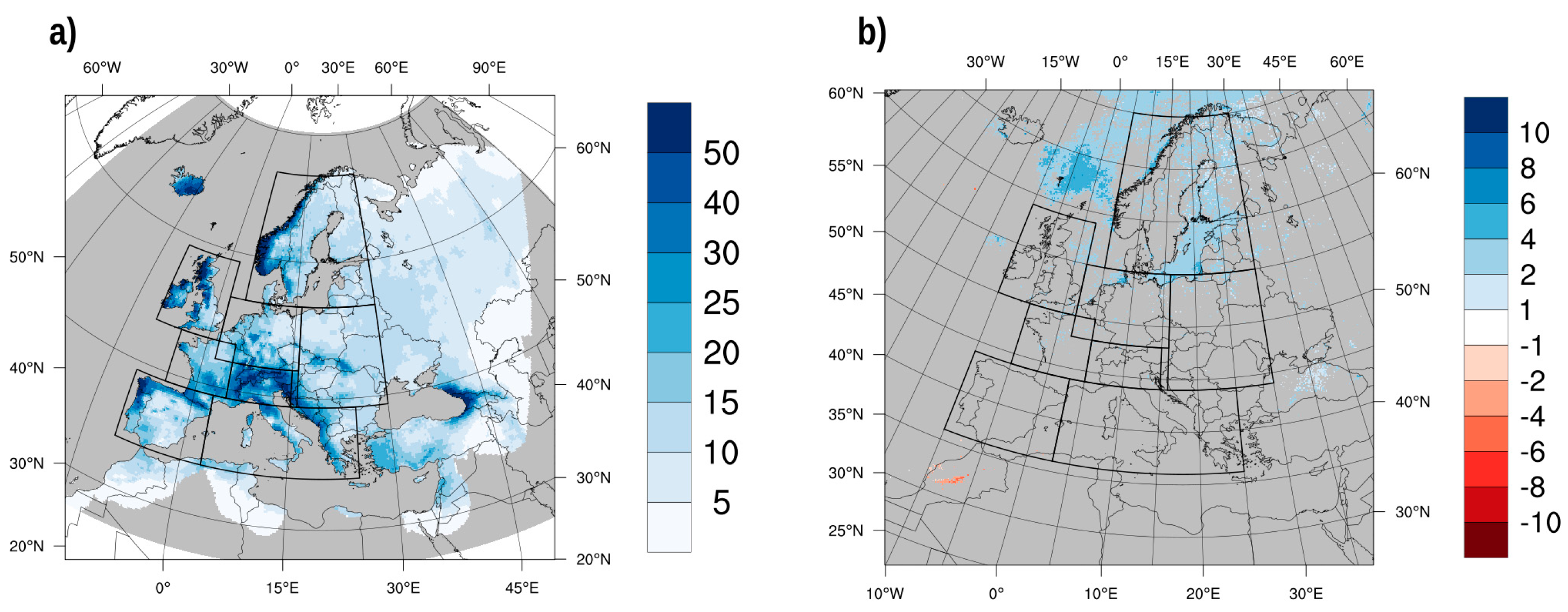
3.2. Tropical Nights

Under present day climate conditions, tropical nights are observed mainly in southern and south-eastern European regions (see Figure 2a). Unlike for hot days, where the affected area covers most of the land parts in the Mediterranean region, tropical nights occur in specific geographical regions, e.g, the southern part of the Iberian Peninsula, parts of Catalonia, coastal regions in southern France, the Po-valley, Southern Italy and coastal areas in Greece and Turkey. The number of tropical nights is mostly about five tropical nights per year but can reach up to 20–40 tropical nights in smaller areas, e.g., in southern Spain.

Even under the +1.5 °C GWL, a substantial increase in the number of tropical nights is projected for southern and eastern Europe (refer to Figure 2b). Those regions with increasing numbers of tropical nights extend slightly northwards under +2.0 °C GWL and even further under the +3.0 °C GWL (see Figure 2c,d for +2.0 °C GWL and +3.0 °C GWL, respectively).

The strongest changes are simulated over the Mediterranean area, with 17.4 (ensemble spread: 11.2 to 25.8) more tropical nights per year under +1.5 °C GWL and with almost the whole population exposed to an increased number of tropical nights, and with 88% of the whole region affected by significant changes. Under +2.0 °C and +3.0 °C GWL, the whole population is exposed to an increase in tropical nights of 24.3 (15.8 to 37.3) and 38.1 (26.6 to 54.4); the area affected by significant changes extends to 93% and 97% of the total area, respectively.

Similarly, over the Iberian Peninsula, almost the whole population is exposed to a large increase in the number of tropical nights in all three GWLs, but with an increase under +3.0 °C GWL, which is with 29.6 tropical nights per year: about three times larger than under +1.5 °C GWL.

In Mid-Europe, the population exposed to an increased number of tropical nights strongly extends from 35% of the total population under the +1.5 °C GWL to 79% under the +2.0 °C GWL and 100% under the +3.0 °C GWL. The increase is 1.2 (0 to 8.5) days per year under +1.5 °C GWL, 1.4 (0.1 to 10.6) under +2.0 °C and 3.8 (0.4 to 17.0) under +3.0 °C GWL. Also, the area affected by those changes increases substantially from 27% of the total area under +1.5 °C GWL to 67% under +2.0 °C GWL and almost 100% under +3.0 °C GWL.

The part of the area of the British Isles which is affected by significant changes in tropical nights is comparatively small, with 1% under +1.5 °C GWL, 5% under +2.0 °C GWL and 33% under +3.0 °C GWL. However, the population that is exposed to those changes increases substantially from almost 0% to 76% under +3.0 °C GWL, as the affected regions in the south are largely populated areas including, among others, the city of London.

In Scandinavia, under +1.5 °C GWL, none of the area and population is exposed to changes in tropical nights, but under +3.0 °C GWL, in 18% of the area in this region, a slight increase of 2 (0.1 to 16.3) tropical nights per year occurs under +3.0 °C GWL, to which 32% of the total population and 51% of the population in urban areas are exposed.

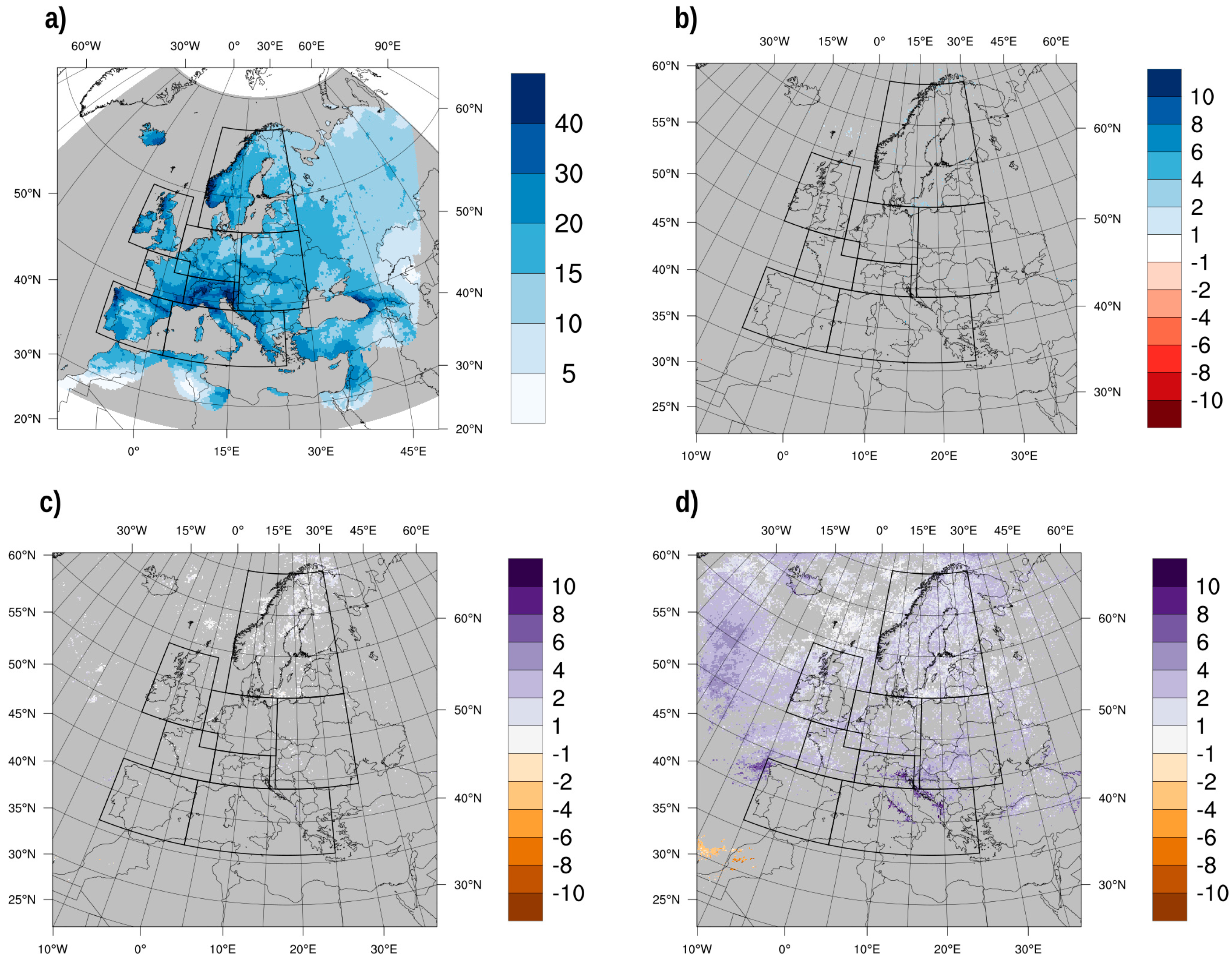
3.3. Dry Days

Under present day conditions as represented in E-OBS, large parts of central and northern Europe experience between 200 and 250 dry days per year (see Figure 3a). Coastal areas in Norway as well as Scotland and Ireland experience less than 200 dry days per year, while in southern European regions, between 250–300 dry days can be observed. Southern Spain exhibits the highest number of dry days with in part more than 300 dry days/year.

Except for Scandinavia, the number of dry days increases in areas where a significant change in dry days is simulated. Over the Iberian Peninsula, even at +1.5 °C GWL a mean increase of 6.8 (2.3 to 12.7) dry days can be observed compared to the reference period. The number of dry days further increases with the GWL to 13.1 (4.4 to 22.6) under +3.0 °C GWL. In parallel, the fraction of the population and area affected by a significant increase raises with each step in GWL: while only 1.2% of the population is affected by an increase in dry days under +1.5 °C GWL, almost 90% of the population are affected under +3.0 °C GWL.

In other regions, a significant change in dry days is simulated only for +2.0 °C and +3.0 °C GWL. The British Isles and France show an increase for +3.0 °C GWL of 9.9 (−5.0 to 19.6) and 9.4 (−7.3 to 18.3) dry days per year, respectively, with a relatively low fraction of the population affected by these changes. No significant changes are simulated for Mid-Europe.

In Scandinavia, a decrease in dry days of −8.4 (−15.6 to 4.7) and −10.0 (−18.6 to 5.1) is simulated for +2.0 °C and +3.0 °C, respectively, with less than 10% of the surface and less than 2.5% of the population affected by those changes as they occur in sparsely inhabited areas.

Figure 3c shows that, under +2.0 °C GWL, additional significant changes in dry days compared to +1.5 °C GWL are present in southern Spain and south-western Turkey. Under +3.0 °C GWL (see Figure 3d), a large part of Spain and the entire Mediterranean area would experience additional increase in dry days. Those regions are experiencing a high level of dry days already today (see Figure 3a). A significant decrease in dry days is only projected for the northern part of Scandinavia, which only appears under +3.0 °C GWL. This decrease is partly present in spring, autumn and winter and can therefore not be related to a specific season (not shown).

3.4. Heavy Precipitation Days

Heavy precipitation days show elevated values in many coastal and mountainous regions in Europe (see Figure 4a). The western coasts of Portugal, Spain, Ireland, Great Britain and Norway especially experience more than 50 heavy precipitation days per year according to E-OBS data. In addition, over the Pyrenees, the Alps, the Apennines in Italy and the western part of the Balkans, elevated values of more than 30 heavy precipitation days can be observed at present.

While for most of Europe a significant change in heavy precipitation days is not visible under +1.5 °C GWL, an increase for parts of Scandinavia becomes apparent (see Figure 4b). The increase in Scandinavia is persistent for all three global warming scenarios, reaching from 2.6 to 4.8 days/year (ensemble spread: 0.3 to 5.1 and 1.6 to 8.8 for +2.0 °C and +3.0 °C GWL, respectively). Also, the affected population and area increases with GWL from about one fourth to nearly the entire population and area, which is affected by a significant change in heavy precipitation days under +3.0 °C GWL.

Interestingly, with increasing GWL the effect of the increasing number of precipitation days spreads from northern to Mid-Europe and eastern Europe. For the +3.0 °C GWL, this effect intensifies: in Mid-Europe, an increase in heavy precipitation days of 3.8 days/year are projected with 88.0% of the population affected. Under +1.5 °C and +2.0 °C GWL, only 3.2% and 17.6% of the population were affected, respectively, with slightly higher values for population living in densely populated areas.

For France, a significant increase in heavy precipitation days/year is simulated for +3.0 °C GWL, where 34.6% of the entire population and 59% of the population in densely populated areas is affected. The reason for the relatively high latter value is that the northern part of France, including Paris is affected. While a small area shows significant changes under +1.5 °C, no significant changes are simulated under 2.0 GWL.

A decrease of heavy precipitation days can be observed over the Iberian Peninsula, where about 21.6% of the population are affected by a mean change of −4.4 (−0.6 to −9.3) heavy precipitation days. Areas affected here are mainly the southern part of Spain and Portugal, the northern coast and the Pyrenees. Also, in small areas of southern Italy and Greece, a decrease in heavy precipitation days is simulated under +3.0 °C GWL.

3.5. 99th Percentile of Precipitation

The 99th percentile of precipitation for wet days gives information about the magnitude of extreme precipitation events per year.

In the present-day climate as represented by E-OBS data, the 99th percentile of precipitation ranges between 5–10 mm/day in central Spain, eastern Germany and large parts of Poland as well as north-eastern Europe to more than 40 mm/day in coastal areas of Norway, western Scotland and south-western Ireland, the west coast of the Iberian peninsula, the Pyrenees and the Alps as well as parts of the northern Balkans (see Figure 5a).

Under +1.5 °C GWL, there are no significant changes in Europe over larger areas simulated (see Figure 5b).

Under +2.0 °C GWL, a larger area is affected by significant changes of the 99th percentile of precipitation only in Scandinavia (see Figure 5c). This is projected to increase by 3.0 (0.0 to 6.0) mm/day, while about 9.3% of the population and 14.3% of the surface are affected. Other European regions are not affected, or only at isolated places.

A major increase in the 99th percentile of precipitation is simulated in various regions affecting a larger part of the population under +3.0 °C GWL (see Figure 5d and Table 4). This is especially the case for Scandinavia, where an increase of 3.7 (0.6 to 7.4) mm/day is simulated, while 61.2% of the population and 69.9% of the surface are experiencing a significant change.

In other regions, e.g., Mid-Europe, 37.7% of the population and 34.1% of the area are affected by a significant change in the 99th percentile of precipitation with a mean change in the area of 3.7 (0.0 to 8.4) mm/day under +3.0 °C GWL. A similar order of magnitude of change in the 99th percentile of precipitation is simulated in France with 4.0 (0.1 to 10.2) mm/day and a population fraction of 25.4% affected by significant changes in the 99th percentile of precipitation. In the Iberian Peninsula region, no larger areas are affected.

From Figure 3d, one can see that additional changes in the 99th percentile of precipitation are scattered over the central and northern part of the continent, with increased values mainly over the Atlantic ocean but also at coastal areas of the west coast of Italy and the west coast of the Balkans, where the maximum changes in the 99th percentile of precipitation is simulated along the Julian and Dinaric Alps.

4. Discussion

As shown in the previous section, temperature and precipitation-related indices simulated by the ensemble used in this study show important differences under the GWLs +1.5 °C, +2.0 °C and +3.0 °C for specific regions.

Concerning temperature-related climate indices, this study shows that the largest absolute increase is simulated for regions that are even today experiencing a large number of hot days and tropical nights. It is present under +1.5 °C GWL and increases even further under +2.0 °C and +3.0 °C GWL. Affected regions are mainly located in southern Europe, i.e., the Iberian Peninsula and the Mediterranean, where the increase is stronger than further north, e.g., France or Mid-Europe. In Scandinavia and the British Isles, only under +3.0 °C GWL are significant changes in hot days and tropical nights simulated, but mainly in their southern areas. Therefore, the north–south gradient which already exists today would intensify with increasing GWL. Many regions are affected equally by an increase of hot days and tropical nights, which might intensify critical climate conditions.

Regions in southern Europe would avoid the largest absolute increase in tropical nights and hot days under +1.5 °C GWL compared to +2.0 °C and +3.0 °C GWL. Other regions such as mid- and northern Europe could avoid the appearance of tropical nights and hot days almost completely under +1.5 °C GWL. Especially in Mid-Europe under +3.0 °C GWL, tropical nights and hot days are simulated to appear regularly. According to this study, most parts of Scandinavia would be the only regions that is not affected by an increase in the two temperature related climate indices investigated in this study.

In many regions, a relatively large fraction of the population is affected by a significant increase in hot days and tropical nights. In some regions in which only a small fraction of the area is affected, such as the British Isles and Scandinavia, an important fraction of the population might experience an increase in temperature-related indices, however. This is due to the higher population density in the southern parts of those regions.

Concerning precipitation-related indices, no clear north–south gradient can be observed under present-day conditions and for projected changes. Overall, for mid- and northern Europe, an increase in precipitation extremes is simulated especially under +3.0 °C GWL, while for southern Europe, an increase in dry days is projected for many regions. This is in agreement with the change characteristic in mean precipitation, which [2] found at +2.0 °C GWL.

Under +1.5 °C GWL, a significant increase of the 99th percentile of precipitation and the heavy precipitation days can be avoided with respect to the reference period 1971–2000. Even under +2.0 °C GWL, the increase in the 99th percentile of precipitation affects less than 15% of the area and less than 10% of the population in each region, while a moderate increase in heavy precipitation days is projected for northern Europe compared to the +1.5 °C GWL.

Considerable differences in changes of precipitation-related indices are projected for +3.0 °C GWL compared to the +1.5 °C GWL. In northern Europe, the 99th percentile increases, while at the same time, more heavy precipitation events are simulated. With nearly no changes in dry days, this indicates a broadening of the tail of the precipitation distribution leading to a larger number and to more intense precipitation events at the expense of regular precipitation events in northern Europe. For some areas in the Mediterranean region, e.g., the western coast of Italy, an increase in the 99th percentile of precipitation is simulated, while the number of days with heavy precipitation shows no changes. This indicates a flattening of the tail of the distribution of precipitation leading not to more but to more intense precipitation events which can be avoided under +1.5 °C and +2.0 °C GWL.

Significant substantial increases in dry days, which are simulated mainly in Southern Europe, can be avoided under +1.5 °C GWL compared to +3.0 °C GWL and partly already under +2.0 °C GWL.

In summary, especially in southern European regions, severe increases in temperature extremes in combination with an increase in dry days can be avoided under +1.5 °C GWL compared to higher GWLs, while northern Europe avoids an increase in heavy precipitation.

Despite the rather comprehensive approach to assess the avoided extremes under +1.5 °C GWL compared to +2.0 °C and +3.0 °C GWL used in this study, we had to make a few choices which lead to some limitations.

First of all, the ensemble spread as represented by the ensemble minimum and maximum of the mean quantities in each region is relatively large compared to the climate change signal. Given the relatively small size of the ensemble, we chose to take the minimum and maximum to show the entire width of the ensemble. With more ensemble members being available in the future, the climate change signal might become more apparent and the ensemble spread can be better represented by the 90th and 10th percentile avoiding outliers that dominate the results. Other experiment setups aim at a better signal to noise ratio by focusing on a large ensemble for shorter time-slices (e.g., the half-a-degree additional warming, prognosis and projected impacts (HAPPI)-project [27]). In this project, 10-year time-slices are calculated for different GWL for 50–100 ensemble members, allowing for a more robust statistical assessment [27]. It would be beneficial to compare the results of the different approaches in the future.

A larger ensemble will also lead to more robust information about the significance of climate change signals for the different indices. The choice of the significance test, on the other hand, has only a minor influence on the area of significant climate change signals for the indices in our setup. In addition to the two-sided Mann–Whitney-U test presented in this study, we examined the choice of a one-sided Mann–Whitney-U test, which lead to slightly larger areas detected as significant, while, when using the two-sided Kolmogorov–Smirnov test [28,29], the area detected as significant is slightly smaller (not shown).

The selection of indices was guided by the idea of presenting the most relevant ones which are related to temperature and precipitation extremes, while limiting its number to be able to show simulated quantitative changes in the regions. This more subjective choice could be broadened to other relevant indices suitable for application in future studies.

5. Summary and Conclusions

In this study, climate change is investigated over the PRUDENCE regions for the GWLs of +1.5 °C, +2.0 °C and +3.0 °C. The study shows the avoidable change in and the avoidable exposure of population of selected climate indices related to temperature and precipitation extremes when keeping global warming below the limit of +1.5 °C.

A +1.5 °C GWL would only lead to a moderate rise in hot days and almost no significant changes in precipitation. Comparing +1.5 °C GWL to +2.0 °C GWL, a further increase in tropical nights and hot days parallel to an increase of dry days in parts of southern Europe as well as an increase in heavy precipitation in parts of Scandinavia could be avoided. Comparing +1.5 °C GWL to +3.0 °C GWL, the benefit of staying at +1.5 °C GWL is even more important. Here, a substantial increase (i.e., an increase of more than five dry days and ten tropical nights) in dry days and tropical nights would be avoided under +1.5 °C GWL compared to +3.0 °C GWL in southern European regions, while in several European regions and especially in northern Europe a substantial increase in heavy precipitation days (i.e., more than two heavy precipitation days) could be avoided.

While climate indices related to temperature extremes increase gradually with increasing GWL, the major difference in precipitation extremes related indices occurs between +2.0 °C and +3.0 °C. To sum up, severe increases in temperature extremes in combination with an increase in dry days can be avoided under +1.5 °C GWL compared to higher GWLs, especially in southern European regions, while an increase in heavy precipitation can be avoided mainly in northern Europe.

With increasing GWL an increasing fraction of the area and similarly an increasing fraction of the population of the respective PRUDENCE regions are also affected by an increase in extreme climate change conditions. There are cases in which a larger increase in the exposed population than in the affected area is projected. This is, e.g., the case for the increase in tropical nights for the British Isles, where parts of highly-populated southern England are exposed to significant changes in tropical nights. This is especially important when considering the costs for adaptation.

In this study, we restrict ourselves to quantifying important changes of single climate indices in different European regions. A combination of multiple extremes (e.g., hot days in combination with dry days) can in particular reinforce themselves and have detrimental influences on human health and ecosystems. The results of this study can be used to identify hotspot regions in which impact models have to be used to assess impacts of climate change.