Evaluation of Analysis by Cross-Validation, Part II: Diagnostic and Optimization of Analysis Error Covariance


Abstract
1. Introduction
2. Theoretical Framework
2.1. Diagnostic of Analysis Error Covariance in Passive Observation Space
2.2. A Complete Set of Diagnostics of Error Covariances in Passive Observation Space
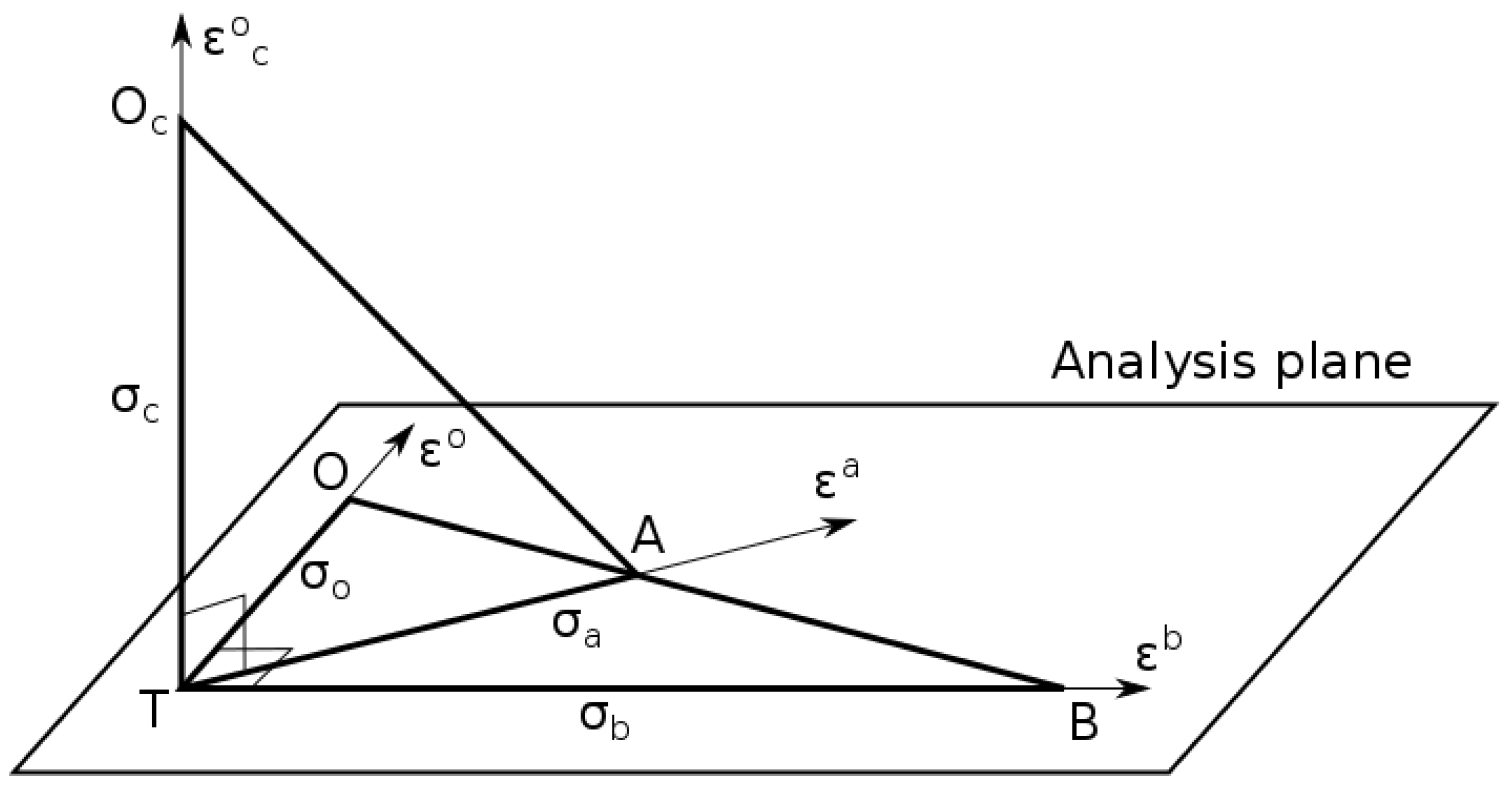
2.3. Geometrical Interpretation
2.4. Error Covariance Diagnostics in Active Observation Space for Optimal Analysis
2.5. Error Covariance Diagnostics in Passive Observation Space for Optimal Analysis
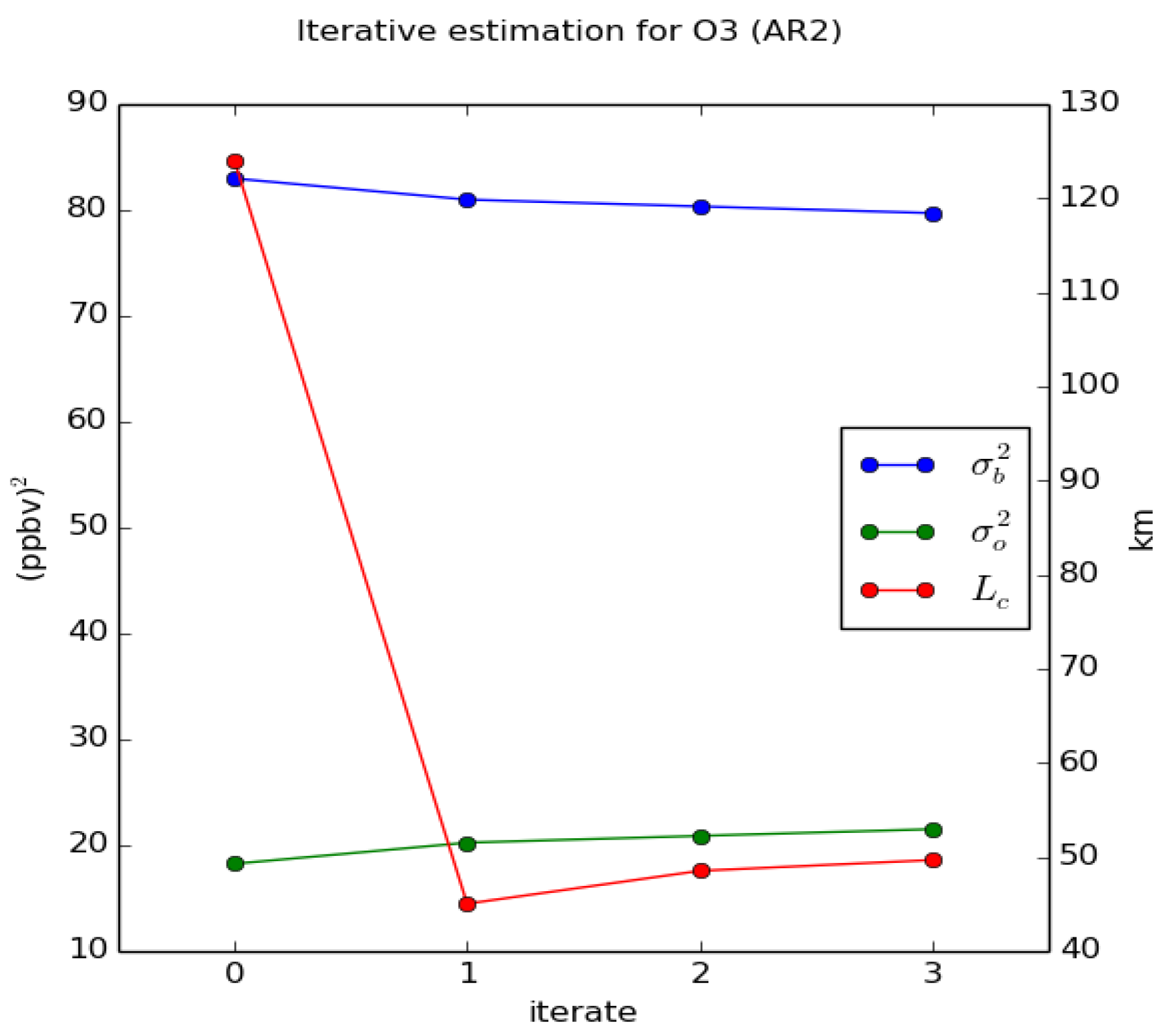
3. Results with Near Optimal Analyses
3.1. Experimental Setup
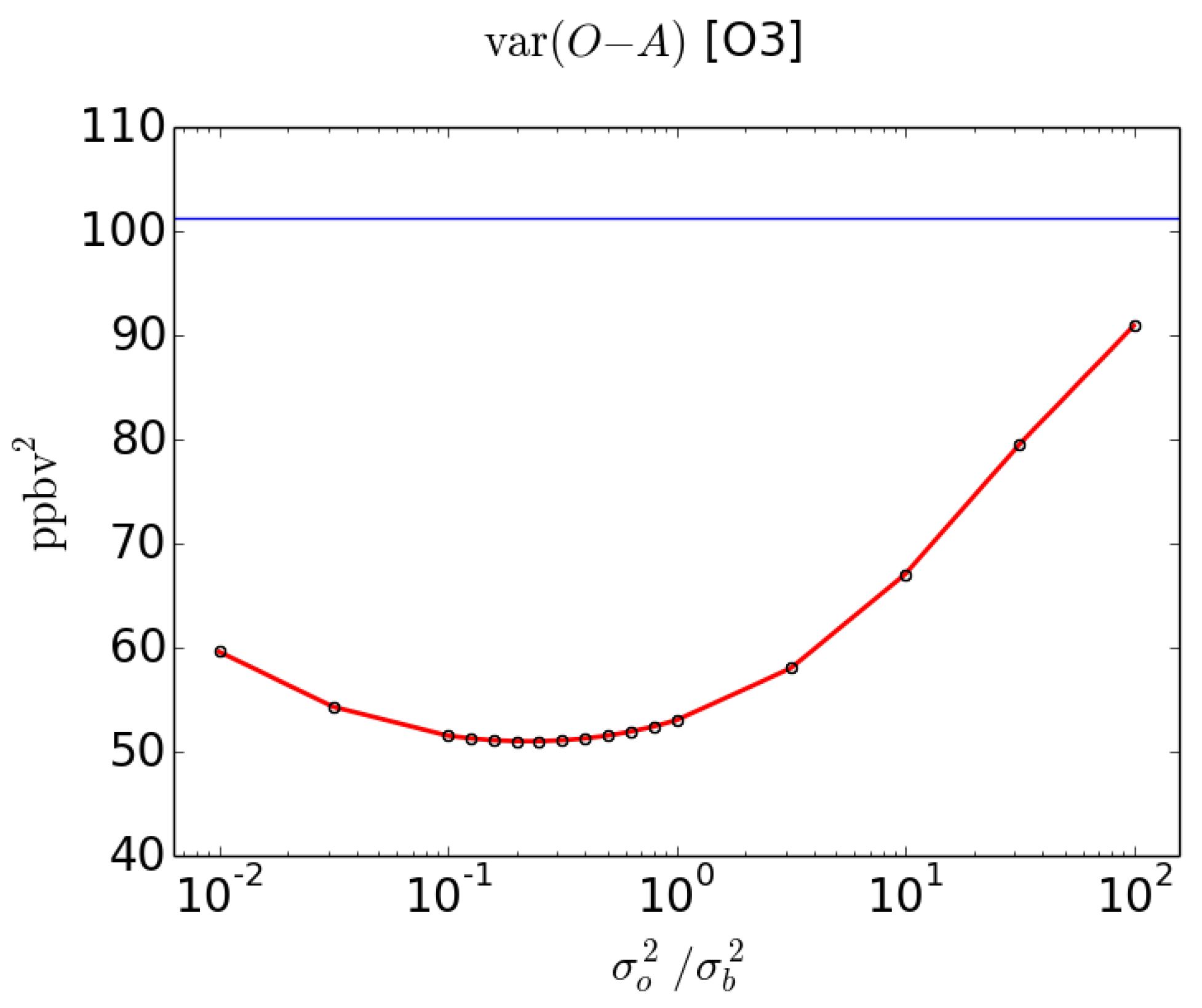
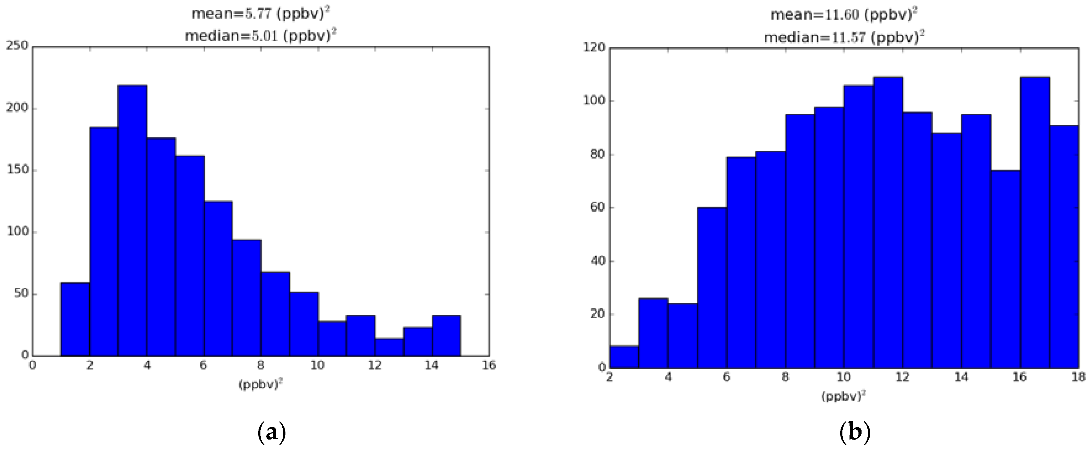
3.2. Statistical Diagnostics of Analysis Error Variance
3.3. Comparison with the Perceived Analysis Error Variance
4. Discussion on the Statistical Assumptions and Practical Applications
4.1. Representativeness Error with In situ Observations
4.2. Correlated Observation-Background Errors
4.3. Estimation of Satellite Observation Errors with In situ Observation Cross-Validation
4.4. Remark on Cross-Validation of Satellite Retrievals
4.5. Lack of Innovation Covariance Consistency and Its Relevance to the Statistical Diagnostics
5. Conclusions
Supplementary Materials
Acknowledgments
Author Contributions
Conflicts of Interest
Appendix A. A Geometrical Derivation of the Desroziers et al. Diagnostic
Appendix B. Diagnostics of Analysis error Covariance and the Innovation Covariance Consistency
References
- Ménard, R.; Robichaud, A. The chemistry-forecast system at the Meteorological Service of Canada. In Proceedings of the ECMWF Seminar Proceedings on Global Earth-System Monitoring, Reading, UK, 5–9 September 2005; pp. 297–308. [Google Scholar]
- Robichaud, A.; Ménard, R. Multi-year objective analysis of warm season ground-level ozone and PM2.5 over North-America using real-time observations and Canadian operational air quality models. Atmos. Chem. Phys. 2014, 14, 1769–1800. [Google Scholar] [CrossRef]
- Robichaud, A.; Ménard, R.; Zaïtseva, Y.; Anselmo, D. Multi-pollutant surface objective analyses and mapping of air quality health index over North America. Air Qual. Atmos. Health 2016, 9, 743–759. [Google Scholar] [CrossRef] [PubMed]
- Moran, M.D.; Ménard, S.; Pavlovic, R.; Anselmo, D.; Antonopoulus, S.; Robichaud, A.; Gravel, S.; Makar, P.A.; Gong, W.; Stroud, C.; et al. Recent advances in Canada’s national operational air quality forecasting system. In Proceedings of the 32nd NATO-SPS ITM, Utrecht, The Netherlands, 7–11 May 2012. [Google Scholar]
- Ménard, R.; Deshaies-Jacques, M. Evaluation of analysis by cross-validation. Part I: Using verification metrics. Atmosphere 2018, in press. [Google Scholar]
- Daley, R. The lagged-innovation covariance: A performance diagnostic for atmospheric data assimilation. Mon. Weather Rev. 1992, 120, 178–196. [Google Scholar] [CrossRef]
- Daley, R. Atmospheric Data Analysis; Cambridge University Press: New York, NY, USA, 1991; p. 457. [Google Scholar]
- Talagrand, O. A posteriori evaluation and verification of analysis and assimilation algorithms. In Proceedings of Workshop on Diagnosis of Data Assimilation Systems, November 1998; European Centre for Medium-Range Weather Forecasts: Reading, UK, 1999; pp. 17–28. [Google Scholar]
- Todling, R. Notes and Correspondence: A complementary note to “A lag-1 smoother approach to system-error estimaton”: The intrinsic limitations of residuals diagnostics. Q. J. R. Meteorol. Soc. 2015, 141, 2917–2922. [Google Scholar] [CrossRef]
- Hollingsworth, A.; Lönnberg, P. The statistical structure of short-range forecast errors as determined from radiosonde data. Part I: The wind field. Tellus 1986, 38A, 111–136. [Google Scholar] [CrossRef]
- Ménard, R.; Deshaies-Jacques, M.; Gasset, N. A comparison of correlation-length estimation methods for the objective analysis of surface pollutants at Environment and Climate Change Canada. J. Air Waste Manag. Assoc. 2016, 66, 874–895. [Google Scholar] [CrossRef] [PubMed]
- Janjic, T.; Bormann, N.; Bocquet, M.; Carton, J.A.; Cohn, S.E.; Dance, S.L.; Losa, S.N.; Nichols, N.K.; Potthast, R.; Waller, J.A.; et al. On the representation error in data assimilation. Q. J. R. Meteorol. Soc. 2017. [Google Scholar] [CrossRef]
- Hollingsworth, A.; Lönnberg, P. The verification of objective analyses: Diagnostics of analysis system performance. Meteorol. Atmos. Phys. 1989, 40, 3–27. [Google Scholar] [CrossRef]
- Desroziers, G.; Berre, L.; Chapnik, B.; Poli, P. Diagnosis of observation-, background-, and analysis-error statistics in observation space. Q. J. R. Meteorol. Soc. 2005, 131, 3385–3396. [Google Scholar] [CrossRef]
- Ménard, R. Error covariance estimation methods based on analysis residuals: Theoretical foundation and convergence properties derived from simplified observation networks. Q. J. R. Meteorol. Soc. 2016, 142, 257–273. [Google Scholar] [CrossRef]
- Kailath, T. An innovation approach to least-squares estimation. Part I: Linear filtering in additive white noise. IEEE Trans. Autom. Control 1968, 13, 646–655. [Google Scholar]
- Marseille, G.-J.; Barkmeijer, J.; de Haan, S.; Verkley, W. Assessment and tuning of data assimilation systems using passive observations. Q. J. R. Meteorol. Soc. 2016, 142, 3001–3014. [Google Scholar] [CrossRef]
- Waller, J.A.; Dance, S.L.; Nichols, N.K. Theoretical insight into diagnosing observation error correlations using observation-minus-background and observation-minus-analysis statistics. Q. J. R. Meteorol. Soc. 2016, 142, 418–431. [Google Scholar] [CrossRef]
- Caines, P.E. Linear Stochastic Systems; John Wiley and Sons: New York, NY, USA, 1988; p. 874. [Google Scholar]
- Cohn, S.E. The principle of energetic consistency in data assimilation. In Data Assimilation; Lahoz, W., Boris, K., Richard, M., Eds.; Springer: Berlin/Heidelberg, Germany, 2010. [Google Scholar]
- Mitchell, H.L.; Daley, R. Discretization error and signal/error correlation in atmospheric data assimilation: (I). All scales resolved. Tellus 1997, 49A, 32–53. [Google Scholar] [CrossRef]
- Mitchell, H.L.; Daley, R. Discretization error and signal/error correlation in atmospheric data assimilation: (II). The effect of unresolved scales. Tellus 1997, 49A, 54–73. [Google Scholar] [CrossRef]
- Joiner, J.; da Silva, A. Efficient methods to assimilate remotely sensed data based on information content. Q. J. R. Meteorol. Soc. 1998, 124, 1669–1694. [Google Scholar] [CrossRef]
- Migliorini, S. On the quivalence between radiance and retrieval assimilation. Mon. Weather Rev. 2012, 140, 258–265. [Google Scholar] [CrossRef]
- Chapnik, B.; Desroziers, G.; Rabier, F.; Talagrand, O. Properties and first application of an error-statistics tunning method in variational assimilation. Q. J. R. Meteorol. Soc. 2005, 130, 2253–2275. [Google Scholar] [CrossRef]
- Ménard, R.; Deshiaes-Jacques, M. Error covariance estimation methods based on analysis residuals and its application to air quality surface observation networks. In Air Pollution and Its Application XXV; Mensink, C., Kallos, G., Eds.; Springer International AG: Cham, Switzerland, 2017. [Google Scholar]
- Skachko, S.; Errera, Q.; Ménard, R.; Christophe, Y.; Chabrillat, S. Comparison of the ensemlbe Kalman filter and 4D-Var assimilation methods using a stratospheric tracer transport model. Geosci. Model Dev. 2014, 7, 1451–1465. [Google Scholar] [CrossRef]
- Efron, B. An Introduction to Boostrap; Chapman & Hall: New York, NY, USA, 1993; p. 436. [Google Scholar]


| Experiment | (km) | |||||
| O3 iter 0 | 124 | 101.25 | 0.22 | 18.3 | 83 | 2.23 |
| O3 iter 1 | 45 | 101.25 | 0.25 | 20.2 | 81 | 1.36 |
| PM2.5 iter 0 | 196 | 93.93 | 0.17 | 13.6 | 80.3 | 2.04 |
| PM2.5 iter 1 | 86 | 93.93 | 0.22 | 16.9 | 77 | 1.25 |
| Experiment | Active | Active | Active | Active | Active |
| O3 iter 0 | 60.29 | 22.69 | 9.61 | 24.33 | −6.03 |
| O3 iter 1 | 67.66 | 13.32 | 13.68 | 11.26 | 8.94 |
| PM2.5 iter 0 | 62.29 | 17.98 | 7.71 | 16.78 | −3.18 |
| PM2.5 iter 1 | 66.3 | 10.68 | 9.51 | 9.57 | 7.33 |
| Experiment | Passive | Passive | Passive | Passive |
| O3 iter 0 | 56.95 | 26.03 | 51.02 | 32.72 |
| O3 iter 1 | 52.04 | 28.95 | 48.95 | 28.75 |
| PM2.5 iter 0 | 62.29 | 22.65 | 38.09 | 24.49 |
| PM2.5 iter 1 | 66.3 | 24.62 | 38.28 | 21.38 |
| Experiment | Perceived |
| O3 iter 0 | 5.77 |
| O3 iter 1 | 11.60 |
| PM2.5 iter 0 | 4.37 |
| PM2.5 iter 1 | 8.21 |
© 2018 by the authors. Licensee MDPI, Basel, Switzerland. This article is an open access article distributed under the terms and conditions of the Creative Commons Attribution (CC BY) license (http://creativecommons.org/licenses/by/4.0/).
Share and Cite
Ménard, R.; Deshaies-Jacques, M. Evaluation of Analysis by Cross-Validation, Part II: Diagnostic and Optimization of Analysis Error Covariance. Atmosphere 2018, 9, 70. https://doi.org/10.3390/atmos9020070
Ménard R, Deshaies-Jacques M. Evaluation of Analysis by Cross-Validation, Part II: Diagnostic and Optimization of Analysis Error Covariance. Atmosphere. 2018; 9(2):70. https://doi.org/10.3390/atmos9020070
Chicago/Turabian StyleMénard, Richard, and Martin Deshaies-Jacques. 2018. "Evaluation of Analysis by Cross-Validation, Part II: Diagnostic and Optimization of Analysis Error Covariance" Atmosphere 9, no. 2: 70. https://doi.org/10.3390/atmos9020070
APA StyleMénard, R., & Deshaies-Jacques, M. (2018). Evaluation of Analysis by Cross-Validation, Part II: Diagnostic and Optimization of Analysis Error Covariance. Atmosphere, 9(2), 70. https://doi.org/10.3390/atmos9020070