Overview of the Model and Observation Evaluation Toolkit (MONET) Version 1.0 for Evaluating Atmospheric Transport Models

Abstract

This paper describes the development and initial applications of the Model and Observation Evaluation Tool (MONET) v1.0. MONET was developed to evaluate the Community Multiscale Air Quality Model (CMAQ) for the NOAA National Air Quality Forecast Capability (NAQFC) modeling system. MONET is designed to be a modularized Python package for (1) pairing model output to observational data in space and time; (2) leveraging the pandas Python package for easy searching and grouping; and (3) analyzing and visualizing data. This process introduces a convenient method for evaluating model output. MONET processes data that is easily searchable and that can be grouped using meta-data found within the observational datasets. Common statistical metrics (e.g., bias, correlation, and skill scores), plotting routines such as scatter plots, timeseries, spatial plots, and more are included in the package. MONET is well modularized and can add further observational datasets and different models.

1. Introduction

Ozone (O₃) and particulate matter smaller than 2.5 μm in diameter (PM_2.5) are among a handful of criteria air pollutants—pollutants the Clean Air Act requires to be monitored and regulated—that are primarily responsible for adverse impacts on human health [1]. Breathing these pollutants is recognized as major causes of acute and chronic respiratory and cardiovascular diseases, and premature mortalities associated with air pollution [2].

In relation to health hazards caused by air pollutants, air quality also has a direct impact on the economy. Trasande et al. [3] found the cost of medical care for preterm births attributable to PM_2.5 exposure to be between $2.43 and $9.66 billion. Ghude et al. [4] demonstrates the economic cost of poor air quality in India to crop yields is estimated to be around $1.26 billion annually. Tong et al. [5] reveals a similar influence to crop yields in the United States (U.S.).

Evaluating model simulations is critical for the development and implementation for forecasting [6]. Evaluation of meteorological and air quality parameters are essential in validating and improving model simulations.

Recently, air quality simulations increased from running for days or weeks to months or years, modeling domains increased resolution, and the use of ensembles greatly increased the amount of model output analyzed. The Community Multiscale Air Quality (CMAQ) modeling simulations, used for air quality and air composition modeling, currently run spanning modeling domains of regional to hemispheric scale and modeling times of days to years resulting in terabytes of model output available for analysis. Conventional methods of data analysis, such as spreadsheets, are not suited for a task this large. There are several model evaluation tools available for evaluating meteorological model simulations but few for evaluating air quality models [7]. Although there are many software packages, such as AMET, or visualization tools, such as Verdi, pycmbs, or Panoply, MONET is built using a single open-source language that retrieves, downloads, and analyses both model and observations on a regional scale. MONET is available on all major computing platforms, i.e., Mac, Linux, and PC, and provides the power of a dedicated programming language such as IDL, MATLAB, or ferret if needed.

The National Oceanic and Atmospheric Administration (NOAA) Air Resources Laboratory (ARL) developed the Model and Observation Evaluation Tool (MONET) to aid in the assessment of the National Air Quality Forecasting Capability (NAQFC) [8,9]. MONET reads, interpolates, and organizes model results to observation sites in both space and time resulting in a fast and flexible method to evaluate air quality modeling simulations. Although MONET was originally created to only evaluate CMAQ simulations, it can easily be expanded to include different model outputs (e.g., the Weather Research and Forecasting model, Next Generation Global Prediction System, and Comprehensive Air Quality Model with Extensions), along with adding additional observational sources (e.g., different ground based networks, satellite observations, and other in-situ observations).

This paper describes the structure and functionality of the MONET Python package (version 2.7). A broad description of MONET will be provided, followed by detailed description of how MONET works. Examples of the analysis products available from MONET will be presented and described. Finally, a discussion and future directions of MONET will be provided.

2. Tool Description

MONET pairs observations and gridded model prediction in space and time. This evaluates the model’s performance for a set of predicted or diagnosed fields such as aggregating nitrous oxide (NO) and nitrogen dioxide (NO₂) into nitrogen oxides (NO_x). MONET is built in Python v2.7+ and is intended to follow object oriented concepts. Each model and observation has a specific object intended to be used for its specific cases. Stemming from such object structures, a verification object that inherits observation and model objects can be created allowing for targeted verification between sets of models and observations. MONET runs interactively or with a simple adaptable Python script.

Most of the dependencies can be obtained using commonly available Python packages, such as the Anaconda Python Package or the Enthought Canopy distribution. MONET uses the pandas Python package [10,11] to enable fast and efficient data manipulation using meta-data available in the observational datasets. Pairing of model and observations is done using the pyresample package, (available online: https://pyresample.readthedocs.io/en/latest/), which uses pykdTree to interpolate. Several interpolation methods are available; nearest neighbor, Gaussian, elliptical weighted averaging, or a user defined method, such as inverse distance weighting. Analysis is done using scipy, numpy, and scikit-learn Python functions, while plotting is achieved with Basemap (for spatial plotting), matplotlib, and seaborn [12,13]. 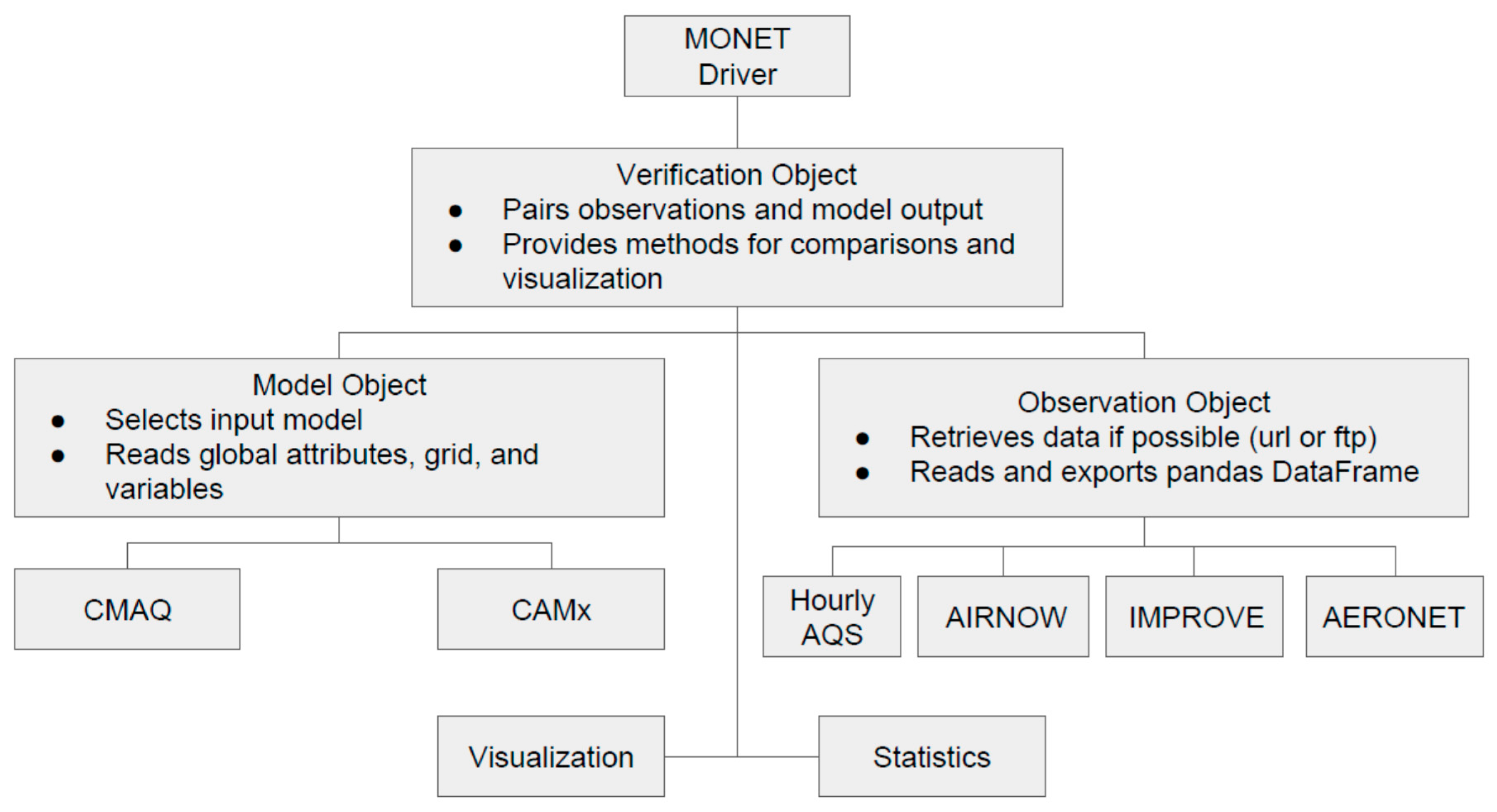Figure 1 presents a flowchart of the MONET software.

MONET runs in four phases; (1) creation of a model object that determines the model grid, variable names, and run duration; (2) creation of an observational object that parses observational data; (3) combines and interpolates model results to observations; and (4) plotting and statistical comparisons.

2.1. Creation of Model and Observation Objects

MONET is designed to be modular in that each observational network or model used has its own set of specialized functions to handle the differences in each dataset. Currently, MONET can handle the hourly Environmental Protection Agency AirData (EPA AQS; available online: https://aqsdr1.epa.gov/aqsweb/aqstmp/airdata/download_files.html#Raw), including the Chemical Speciation Network (CSN) and AirNow (available online: https://www.airnow.gov) datasets, along with the Interagency Monitoring of Protected Visual Environments (IMPROVE; available online: http://vista.cira.colstate.edu/improve) and Aerosol Robotic Network (AERONET; available online: http://aeronet.gsfc.nasa.gov) datasets. Datasets can be readily downloaded through an FTP or http by using an array of datetime objects given to the observation object. Other networks, such as IMPROVE, require that the data be downloaded manually.

Each observation network is designed to monitor specific sets of air quality parameters, from individual pollutants to derived physical parameters (e.g., AOD). MONET makes it easy to compare individual pollutants or to aggregate model results to pair with the monitor dataset. Examples of this are NO_x (NO + NO₂) in AQS or AIRNOW or particle sulfate, an aggregate of the Aitken, accumulation, and coarse mode contribution to the sulfate particle concentration within CMAQ, from AQS and IMPROVE. MONET includes a set of standard aggregations for different pollutants but is versatile enough to allow user defined aggregations.

The observation objects require that a time range is given as an array of datetime objects to the object instance attribute. This is used to tailor data extraction from a pre-downloaded file covering the prescribed time range or otherwise expand the data retrieval. Then, observation objects read the raw datafile and process it into a pandas DataFrame, thus assigning it to an object instance with common columns of observational data (Obs), date (datetime), local date (datetime_local), latitude (Latitude), and longitude (Longitude). Depending on the network, more meta-data may be available, meaning that an observational object in MONET can be used as a standalone method to analyze observational data without the need for pairing. If adding a new network, only the latitude, longitude, observations, and date or timestamp is needed for the interpolation.

For model objects, the only information needed is the output file(s). In the case of overlapping simulations, the model results with the latest creation time stamp will be used. For instance, if two 48 h simulations with 24 h of overlap are given to MONET, then the first 24 h from the first simulation and the 48 h of the second day are used. MONET assigns the model object file to a class instance attribute and creates corresponding helper functions, such as that defining map projections for spatial plotting and retrieving and aggregating data. In the future, the model object will be done with the xarray Python package to keep a consistent view with observations. The xarray package is an N-Dimensional implementation of the pandas library that is highly suitable for scientific data that allows for larger then memory computations and efficient data extraction and resampling.

2.2. Pairing Observations and Model Results

MONET has a built-in driver for each model and observation pair, meaning that the model and observation are separately imported objects. This creates a simple and efficient method for adding new model results—once a model and observational dataset has its own Python object it can easily follow the same pairing algorithms. The driver creates the model object, reads the time range, and creates the model instance. The model time range is then provided to the observational object, where the data is downloaded and processed into a pandas DataFrame or loaded from a preprocessed file.

At this point, each species available in observations and model prediction are paired. MONET has the ability to calculate or aggregate data, such as the calculation of PM_2.5 (particulate matter with diameter less than 2.5 μm) mass concentration, from several modeled chemical species. Herein, a helper function retrieves the data in the model object to derive the needed data array. MONET then interpolates the model results for each timestamp that is available in the observational network to the observational site and merges them into a common pandas DataFrame containing pairings of model results and observations for all specified observation locations.

The Pyresample library (available online: https://pyresample.readthedocs.io/en/latest/) interpolates the model to observations. Pyresample uses (k-dimensional) KDTrees to transform data defined in one geometrical grid to another. Resampling uses the nearest neighbor, Gaussian, or a customized method, such as inverse distance weighting. MONET allows the user to define the radius of influence and number of neighbors to be used for data re-gridding.

After re-gridding, depending on the dataset, MONET resamples in time and then assigns these processed data to a separate pandas DataFrame for deriving certain species, such as the 8 h max ozone or the daily PM_2.5 concentration. Timing for opening model results, processing of observation data, and pairing takes less than 3 min with AIRNOW for a 48 h simulation. At this point, MONET proceeds to analyze the dataset with the observation and model result pairs.

3. Example of Tool Applications

MONET is a new software package developed for verifying the NAQFC and more generally the CMAQ model. It has been newly developed as described above and is available on GitHub. Detailed examples and installation instructions are available at https://github.com/noaa-oar-arl/MONET. Once MONET makes the verification object, all of the non-spatial plots, such as timeseries, scatter plots, and histograms, are executed through as a single line-command with flags specifying the user’s selection of geographical extent and variables to be plotted. For instance, a user can specify that the geographical extent of their plot be within the U.S. EPA defined Conterminous United States (CONUS) region. MONET performs verification within the entire domain, a region, a state, a county, a metropolitan area, or a specific site. MONET also compares multiple simulations on a single figure simply by creating two verification objects and passing the figure handle. Figure 2, Figure 3, Figure 4, Figure 5 and Figure 6 showcases some of the plotting routines found within MONET.

As an example of how easily MONET does a quick pairing and analysis, the following example shows how to use MONET to pair AirNow data and a CMAQ simulation. Begin by entering an interactive python session.

ipython –pylab

(1)

Import the MONET object. This is the python object interface to the model and observation objects.

import monet

(2)

Set the concentration file or files, in this case concfiles, and the gridcro2d file, gridcro.

concfiles = ‘/path/to/concentration/files/ *.ncf’

(3)

gridcro = ‘/path/to/gridcro2dfile.ncf’

(4)

Use the MONET object to pair the AirNow data and CMAQ simulation by creating an instance of the verified airnow object, which imports both the CMAQ and AIRNOW objects.

m = monet.vairnow (concobj = concfiles, gridobj = gridcro)

(5)

MONET retrieves the observations if not in the current directory and the model is interpolated in space to the observational data points. The paired data can be accessed through the pandas DataFrame contained within the monet object, m.

m.df.head()

(6)

Then simple commands can be used to create different plots. For example, MONET creates a timeseries plot averaged over all of the observations found within the modeling domain with a simple one line execution as follows:

m.compare_param (param = ‘OZONE’, timeseries = True)

(7)

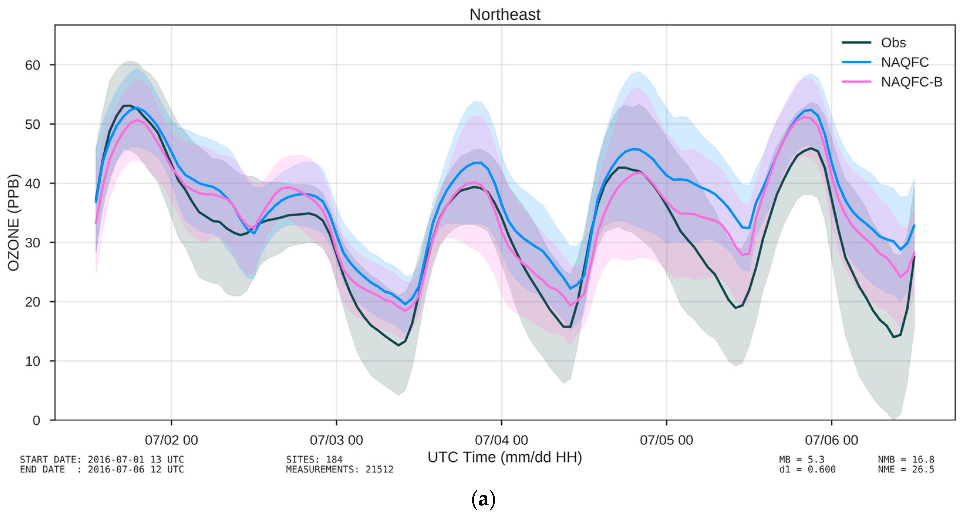
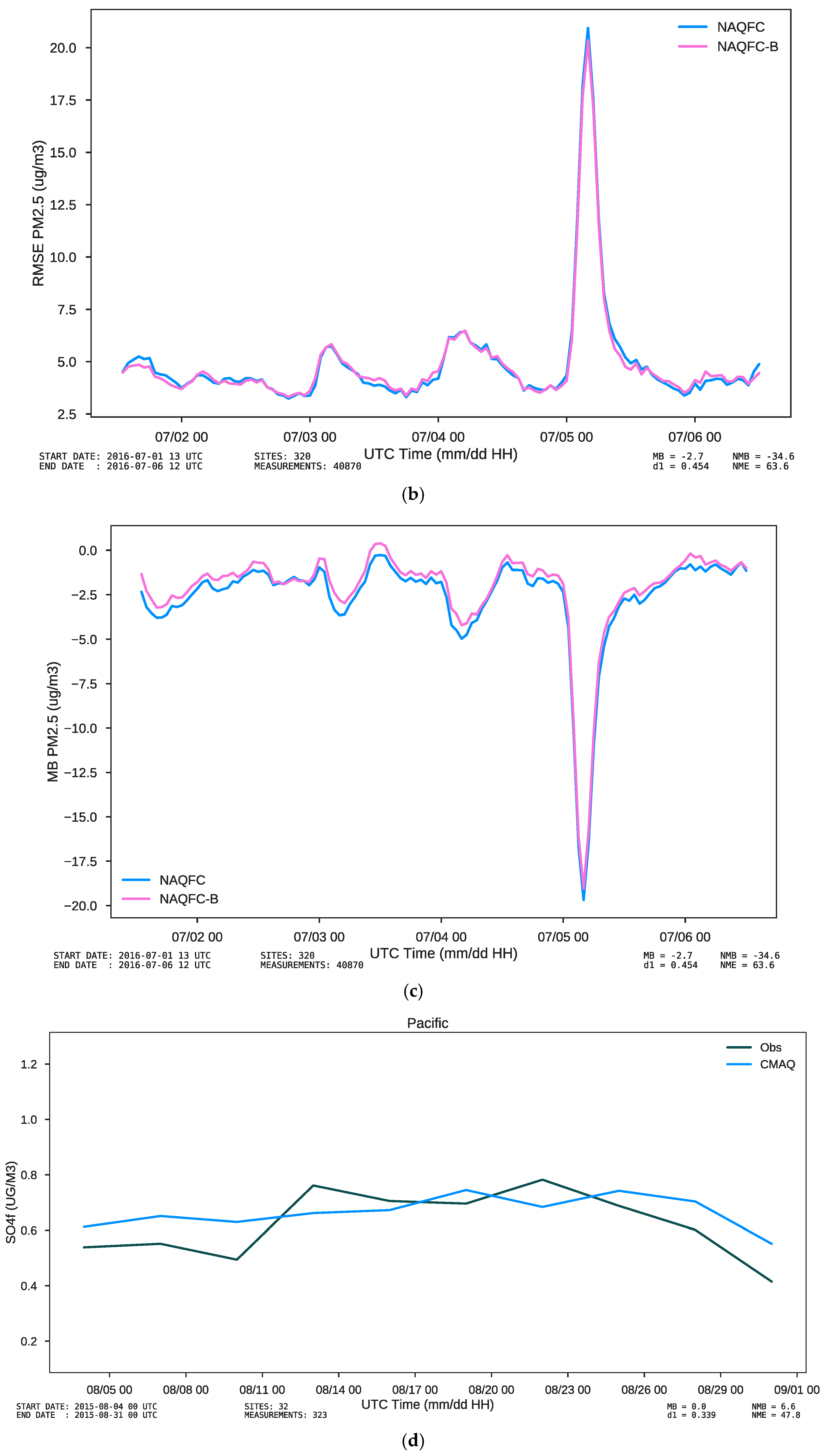
Figure 2a–d shows a time series of the average concentration over the northeastern United States during the summer of 2016. The average value is shown in solid lines, observations in black, and model results in blue and purple. Shaded areas display one standard deviation from the mean. The footer illustates forecasting performance statistical measures specified by the user. The footer also shows the start date, end date, number of sites, and the number of measurements. Figure 2b presents an example of time series root mean square error plot comparing how two simulations performed for the EPA AQS sites in the U.S. EPA CONUS domain. Likewise, Figure 2c displays a mean bias time series of the two simulations. Figure 2d provides an example of speciated PM_2.5 sulfate using the IMPROVE network over the Pacific region. With the IMPROVE network daily average measurement every three days, MONET interpolates the hourly CMAQ results to each individual site and then averaged to create a daily concentration as if were an IMPROVE measurement. Then, MONET merges the daily averaged CMAQ results into the IMPROVE DataFrame using a mysql like merge found within Pandas.

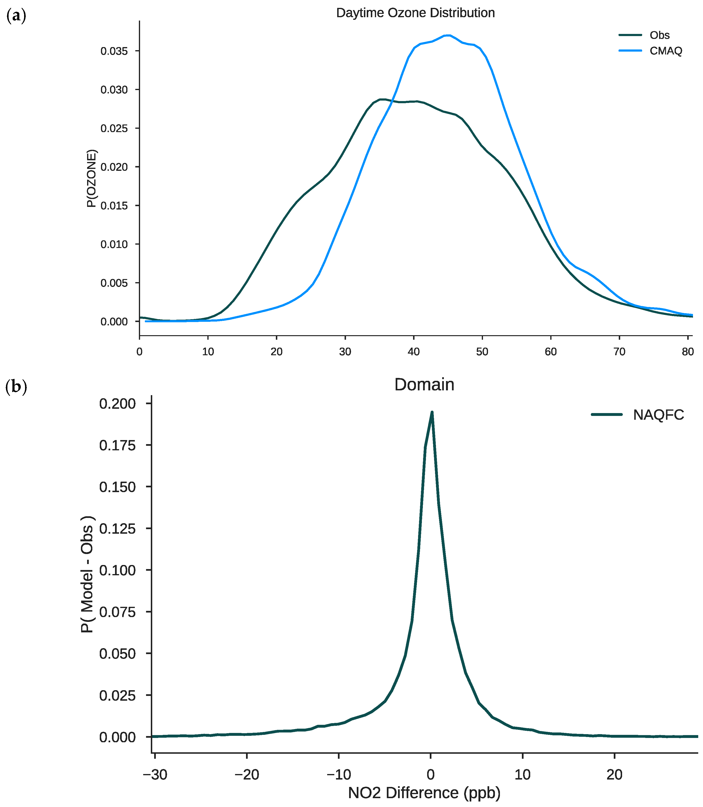
Figure 3a presents an example of a kernel density estimation (KDE) comparison. The black line shows an observational KDE and the blue represents the CMAQ model results. This type of plot (Figure 3a) is useful for inspection for distributional discrepancy between the model and observations. Using conditional distributions, such as conditioning on time of day or other meteorological factors like boundary layer height or wind speed, one can provide a more in depth analysis using MONET. Figure 3b displays the difference in the KDE between model and observation results. Difference KDE are important to show model biases in the most probable value.

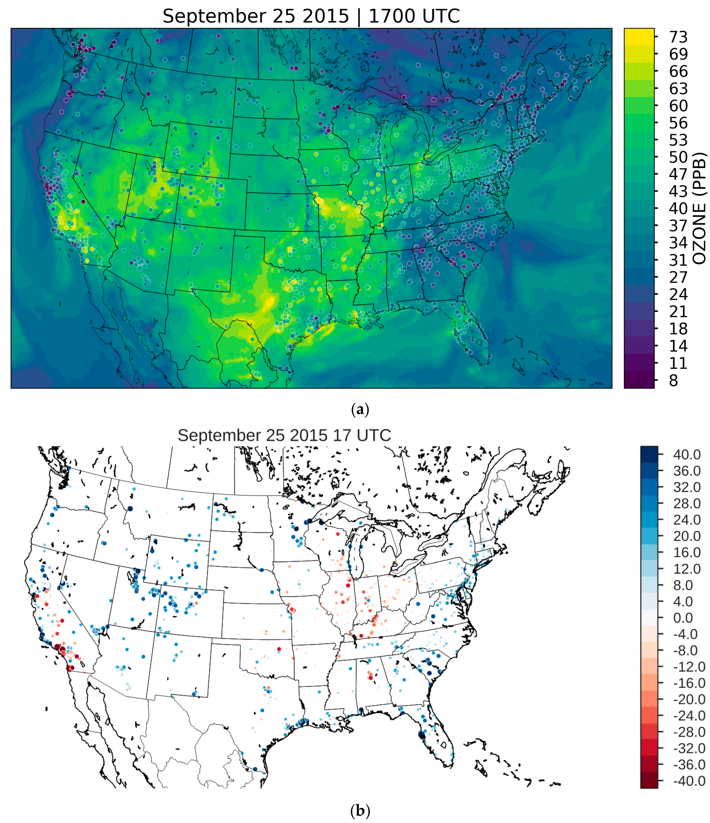
Figure 4a shows an example of a spatial plot of model results against overlaid observations. The colorbar is customizable by passing colormaps that can be user defined or predefined in matplotlib. The colorbar levels can be tailored individually to any single observation. By default, the colorbar is scaled automatically based on the model data and a discrete colorbar with 15 value bins using the ‘viridis’ colormap. The ‘viridis’ colormap is perceptually uniform and sensitive for colorblind individuals. Keyword arguments for the matplotlib.pyplots.imshow can be passed to the MONET function to give additional control over the spatial plot. Spatial plots are useful to give quick glimpses of spatial patterns found within the model. Figure 4b shows an example of a spatial difference plot which is useful for providing spatial assessments for absolute discrepancy. The same type of plot can be created for different metrics such as for RMSE or correlation. In this particular example, it is easy to pertain that over large cities such as Los Angeles or Las Vegas there is a significant under prediction of ozone.

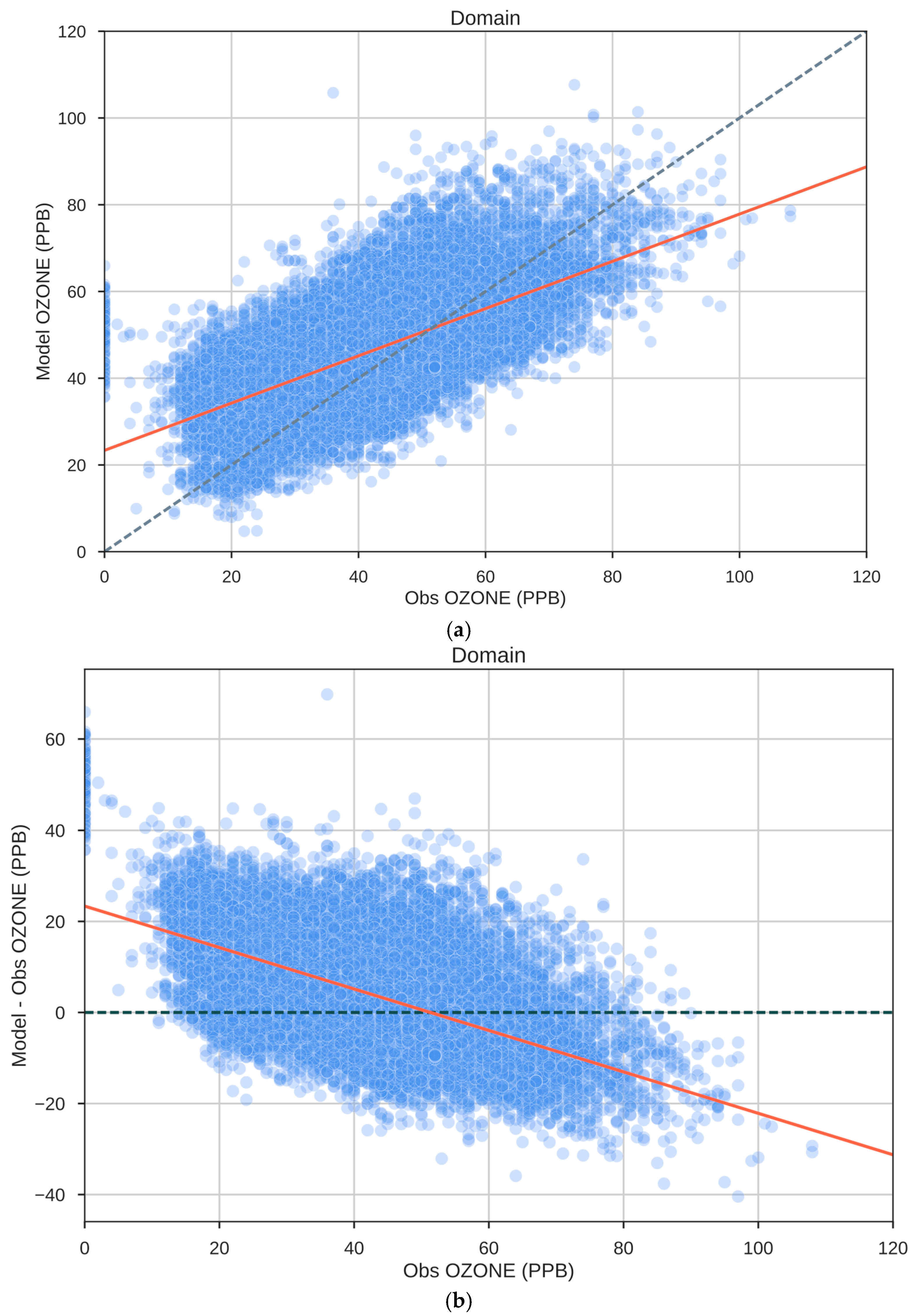
Figure 5a presents a scatter plot, while Figure 5b shows a difference scatter plot. Observations are displayed on the x-axis and model results on the y-axis. A one to one line is automatically created along with a line of best fit. The scipy linregress function creates the line of best fit. Currently, there is not a more complicated fitting algorithm available in MONET. The full power of scipy and scikit-learn is available however if a more in-depth analysis is needed and hopefully will be included in a future version of MONET. This type of plot is useful for determining the correlation of simulation to observational results.

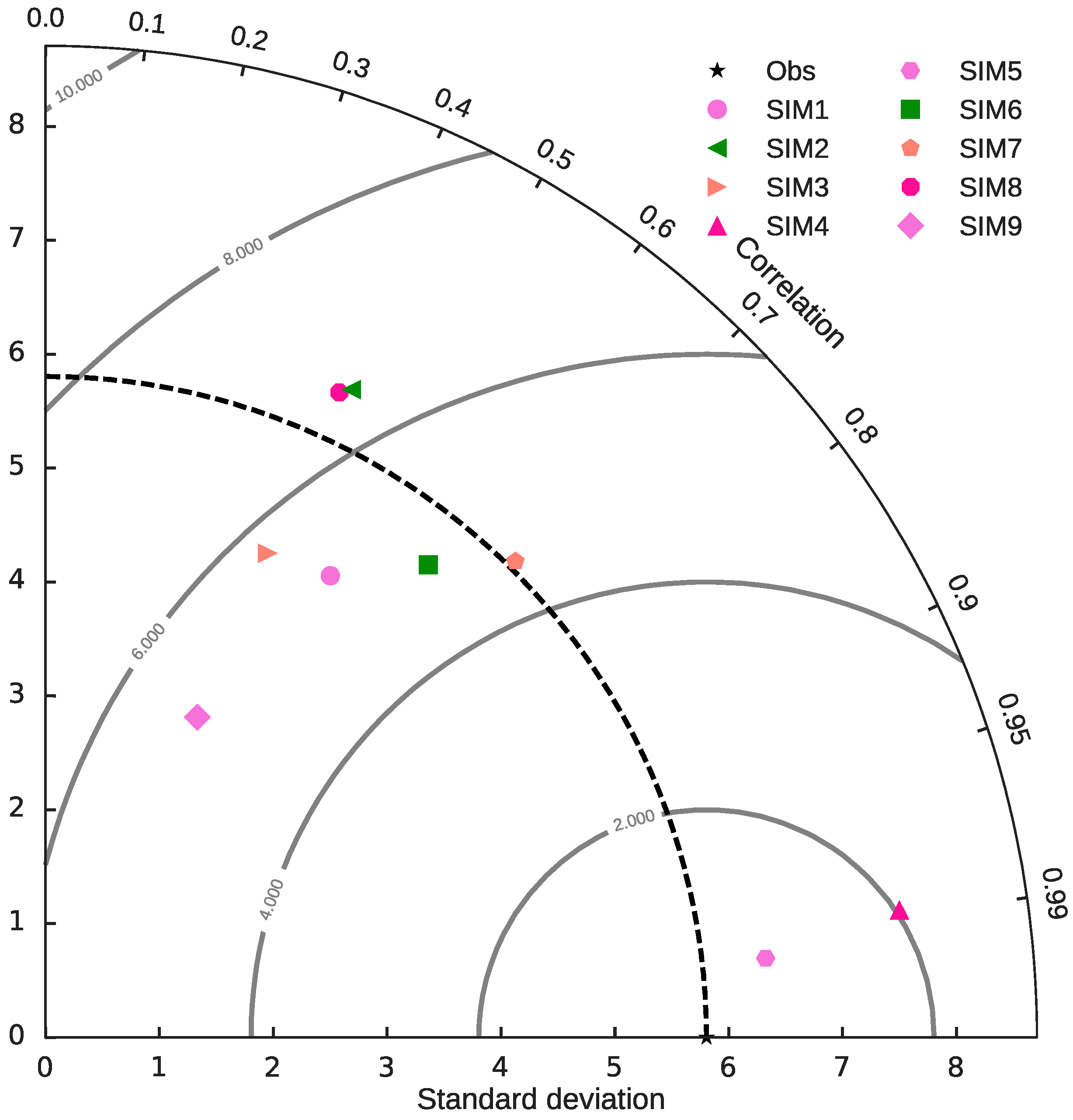
MONET uses the correlation, centered root mean square error, and the standard deviation measures to graphically display on its Taylor diagrams [14]. Taylor diagrams are an efficient way to graphically summarize model performance with observations. Currently, it is up to the user to ensure that data is close to a Gaussian distribution.

The relative merits of various model simulations can be inferred from Figure 6. Simulations that best compare to observations lie closest to the x-axis and have a low RMSE, while simulations that lie above the x-axis have a greater RMSE and lower correlation. The concentric arcs around the observation point show RMSE (in this graph at approximately 5.9 on the x-axis). Dispersion or variation within the simulations are graphically displayed by the distance from the concentric arcs. Simulations closest to the dotted arc have a standard deviation similar to observations.

In this example, SIM5 performed the best as it has the highest RMSE, correlation, and a respectable standard deviation as compared to observations. SIM9 has the lowest standard deviation and SIM2 and SIM8 have the lowest RMSE.

Different visualizations are being developed for future use. Specifically, cumulative distributions, spectral density analysis, and principle component analysis will be added. The addition of different observational data is also a high priority for use with MONET, including data from radiosondes, aircraft, ceilometers, and satellite data. MONET is a simple, easy to use object oriented approach for analyzing model results initially from NAQFC and more generally the CMAQ model.

4. Software and Data Availability

MONET is available on GitHub (https://github.com/noaa-oar-arl/MONET) as a free download. The verification package is written in Python v2.7+. The authors recommend the Anaconda Python package, available for free at https://www.continuum.io/downloads, to install supporting packages described in the readme file included at GitHub. As mentioned previously, MONET uses the Pandas python package to manipulate and store intermediate files. For one day of paired data, the file size is approximately 100 mb for all of the variables and meta-variables in AirNow within the NAQFC domain. MONET uses freely available observational data from the U.S. EPA, U.S. NOAA, U.S. NASA, and U.S. NPS.

5. Conclusions

MONET is a comprehensive software package used to analyze observational data alone or pair observations with gridded model data for chemical transport models. Currently, the observational datasets included are focused within North America, except for AERONET, which is global. MONET performs statistical calculations and creates visualizations to enable researchers to evaluate and improve the scientific understanding of model outputs and observational data. MONET is built entirely on open-source software and while the only model available for use is CMAQ used in the NAQFC, the software is easily able to include different models. To include a new model into MONET, a new object needs to be written that can: (1) read the output and (2) map of the output variables to observation variables needed to pair data; (3) provide an output latitude and longitude for interpolation. Work is ongoing to add the Comprehensive Air Quality Model with Extensions (CAMx) [15] model output to the MONET software package through the use of PseudoNetCDF (https://github.com/barronh/pseudonetcdf).

The MONET software package will continue to grow and improve through internal development at NOAA ARL, and external development through collaborating partners and contributions made through the community. The authors encourage collaborations with intergovernmental agencies, private industry, and academia to improve and further develop MONET. Major software developments are planned for the next release of MONET. One improvement is the inclusion of different models, such as the Weather Research and Forecasting (WRF), CAMx, and the Next Generation Global Prediction System (NGGPS). The next major development planned for MONET is to add different observational sources such as radiosonde, profiler, and radar observations from the Meteorological Assimilation Data Ingest System (MADIS; available online: http://madis.noaa.gov) and AWIPS II (available online: http://www.unidata.ucar.edu/software/awips2/). Another improvement planned is the use of pyresample to re-grid satellite swath data to model grids, as well as calculate comparable variables (e.g., column aggregated aerosol optical depth values from model output).

Analysis enhancements to the MONET software will include implementing non-parametric analysis techniques, such as cumulative distribution frequency plots, and Q-Q plots; adding temporal decomposition capabilities such as Kolmogorov-Zurbenko filtering (Rao and Zurbenko [16]; Wise and Comrie [17]) and spectral density plots; improving the overall speed through the use of parallel processing in pyresample for spatial re-gridding, xarray for temporal averaging, and dask for larger than memory computations. Many improvements to the MONET software are in progress and will be included in the next release.