Abstract
Buildings and vegetation alter the wind and pollutant transport in urban environments. This comparative study investigates the role of orientation and shape of perimeter blocks on the dispersion and ventilation of traffic-related air pollutants, and the street-level concentrations along a planned city boulevard. A large-eddy simulation (LES) model PALM is employed over a highly detailed representation of the urban domain including street trees and forested areas. Air pollutants are represented by massless and passive particles (non-reactive gases), which are released with traffic-related emission rates. High-resolution simulations for four different city-block-structures are conducted over a 8.2 km domain under two contrasting inflow conditions with neutral and stable atmospheric stratification corresponding the general and wintry meteorological conditions. Variation in building height together with multiple cross streets along the boulevard improves ventilation, resulting in 7–9% lower mean concentrations at pedestrian level. The impact of smaller scale variability in building shape was negligible. Street trees further complicate the flow and dispersion. Notwithstanding the surface roughness, atmospheric stability controls the concentration levels with higher values under stably stratified inflow. Little traffic emissions are transported to courtyards. The results provide urban planners direct information to reduce air pollution by proper structural layout of perimeter blocks.
1. Introduction
Decreased air quality is one of the major environmental challenges urban areas are facing today. An increasing number of people are exposed to high air pollution levels due to the ongoing intense urbanisation [1]. Exposure to air pollution has several acute and chronic health effects including respiratory and cardiovascular diseases that further increase mortality (e.g., [2,3]). To illustrate, in 2016 around 4.1 million premature deaths worldwide [4], of which almost 10% in Europe [5], were linked to exposure to elevated concentrations of ambient air pollution.
In urban areas, road traffic accounts for a significant share of the local air pollutant emissions (e.g., [6]). If the prevailing wind conditions within the street canyons lead to inefficient transport and mixing of air, the traffic emissions can accumulate and have longer residence times near the ground level. Consequently, the highest pollution levels within the street canyons are commonly observed at pedestrian level [7]. In order to reduce human exposure to air pollutants within urban areas, the mechanisms affecting the dispersion conditions at street level must be understood and thereby examined in greater detail. To this end, the study of ventilation becomes of critical importance as it addresses the capacity with which a densely built urban structure is capable of replacing the contaminated air with ambient fresh air. Here, ventilation is recognised as a transport process that improves local air quality and closely relates to the term breathability [8,9]. The efficiency at which street canyon ventilation occurs depends on the complex interaction between the atmospheric boundary layer (ABL) flow and the local urban structures. Recognising that the structural layout of urban landscape plays a critical role in determining the local urban air quality, opens up the possibility for the urban planners to incorporate air quality considerations into structural urban design. However, this necessitates sufficiently detailed modelling solutions to address the problem of street canyon ventilation at the scale of individual structures, such as perimeter blocks which are ubiquitous in European cities.
The current capacity to examine street canyon ventilation relies mainly upon parametric models, wind tunnel simulations and field measurements [7]. Parametric models are computationally inexpensive but have decreased accuracy and their applicability is limited to very simplified model set-ups. Reduced-scale wind tunnel simulations, in turn, can suffer from similarity constraints, and field measurements from uncontrollable and unrepeatable boundary conditions and inability to account for spatial variability [10]. Recently, along with rapidly advancing computer power, the application of computational fluid dynamics (CFD) using either models based on the Reynolds-averaged Navier-Stokes equations (RANS) with parametrised turbulence or the large-eddy simulation (LES) method has increased. CFD models provide complete and full-scale three-dimensional flow and concentration fields, which is a major advantage in real and complex urban areas. Majority of the previous urban CFD studies have employed the RANS method, owing to its lower computational costs. Nonetheless, LES outperforms above a complex urban surface due to its ability to resolve instantaneous turbulence structures (e.g., [11,12,13]) also when taking street trees into account [14].
Most of the urban LES studies have considered an idealistic two-dimensional street canyon or a simplified urban topography without including the aerodynamic impact of street trees (e.g., [15,16,17]). This simplification can be dangerous as porous trees decelerate the flow and generate turbulence (e.g., [18]) as well as influence the canyon vortex [19] that is commonly observed in idealised street canyons [20]. Thereby, trees can modify the vertical transport of air pollutants within street canyons [21,22,23,24]. Thanks to the availability of detailed urban topography and land use datasets [25,26], the application of LES to real urban environments (e.g., [27,28,29,30,31]) and also to directly support urban planning [32] has become possible over the last decade. In these cases the computational domain has several requirements to meet. Firstly, the computational domain has to be large enough to capture all relevant turbulence scales (e.g., [33]) and to minimize uncertainties related to the domain boundary conditions [11]. Furthermore, it is assumed that the whole ABL should be included vertically. Secondly, the grid spacing has to be small enough to explicitly resolve the turbulence scales containing most of the energy [31], which requires large computational resources.
The few ventilation studies conducted over a real urban surface [30,32,34] have applied a simple, indirect ventilation indicator, velocity ratio , i.e., the ratio between the wind velocities at pedestrian level (height z = 2 m above ground level (a.g.l.)) and at the top of the model domain , where the flow is no longer influenced by the urban surface, rather than having examined the pollutant concentration, and processes of ventilation and dispersion together in more detail. This study employs an LES model, coupled with a Lagrangian stochastic particle model, to perform high-resolution urban flow simulations in order to answer: How does the structural layout of densely arranged building blocks along a city boulevard influence the ventilation of the local traffic emissions? The accumulation and ventilation of traffic-related air pollutants are investigated in four virtual city-block-design alternatives that are immersed within a real complex urban environment. The question is approached by quantifying and comparing the ventilation efficiency within perimeter blocks using three different measures of air pollutant ventilation and dispersion that are more sophisticated than : concentration, vertical turbulent transport and dilution rate of Lagrangian particles that represent non-reactive gaseous air pollutants. The ventilation measures are further examined in parallel. Simulations are conducted applying two contrasting meteorological conditions for the inflow.
2. Methods
2.1. Model Description
The LES model employed is the Parallelized Large-Eddy Simulation Model (PALM) version 4.0 (revision 1904) for atmospheric and oceanic flows [35,36], which solves the three-dimensional fields of wind and scalar variables (e.g., potential temperature and scalar concentrations). PALM has been applied to various types of ABL studies, for example to study cloudy boundary layers (e.g., [37]), the aerodynamic impact of a plant canopy (e.g., [38]) and stable boundary layer [39]. The performance of PALM over an urban-like surface has been validated against wind tunnel simulations, previous LES studies and field measurements [28,29,30,40]. The aerodynamic impact of vegetation is taken into account in PALM by means of an embedded canopy model. Vegetation decelerates the flow due to the form and viscous drag forces, and the decelerating force depends on the wind velocity and plant area density (, m m). Despite the model has previously been developed for continuous vegetation, it has also been used for individual trees (e.g., [19,41]). For this study, the canopy model was revised to allow a heterogeneous distribution of tree canopy.
Technical specifications of PALM are represented in Appendix A. As a new feature in PALM, a full three-dimensional two-way self-nesting is utilised for the first time [42]. In the nesting approach, a “child” computational domain with chosen grid spacing and dimensions is defined inside the “parent” computational domain. PALM is run in parallel in both domains with respective computational set-ups (Table 1) and the domains communicate with each other. Nesting enables to have both a large computational domain and high enough resolution in the main area of interest without making the simulation computationally too expensive.

Table 1.
The boundary conditions of the model runs. Details of the conditions can be found in Maronga et al. [35].
Ventilation of traffic-related air pollutants is studied by applying a Lagrangian stochastic particle model (LPM) [35]. LPM allows studying pollutant accumulation inside urban structures as concentration values can become higher than at the source unlike in the commonly used Eulerian method (e.g., [31]) due to the maximum principle for scalar conservation laws (e.g., [44]). In LPM, Lagrangian particles are released inside assigned source volumes at selected moments in time, after which they are transported inside the computational domain by the flow field solved by PALM. In this study, Lagrangian particles are defined passive and massless, and hence they represent non-reactive gaseous air pollutants. As for reactive gases and aerosol particles, chemical reactions and dynamic processes manipulating the concentrations should be included. Furthermore, deposition of air parcels on surfaces is not considered here. LPM in PALM was revised for this study to allow for the horizontal heterogeneity and relative strengths of air pollutant sources, i.e., streets with traffic. Particles are released at a selected height with a constant release rate Q (s m), whereas the horizontal locations and group numbers i () of different sources are read from an input file. In order to consider the difference in emission strengths, each source group i can be given a weighting factor and the weighted particle concentration is then calculated as
where is the particle concentration inside a grid box. Weighting method is applied in order to utilise the same, sufficiently high, particle release rate throughout the source area. This approach allows LPM to represent a nearly continuous emission source everywhere without the need to utilise an excessive number of particles there where emissions are high.
2.2. Model Construction
2.2.1. Modelling Area
The simulations are conducted in western Helsinki on a city boulevard that is planned to be built in the new City Plan of Helsinki for 2050. The boulevard will be framed by a densely built neighbourhood, and in this study, four different city-block-design versions are being investigated. The design versions V, where type is either par (parallel), per (perpendicular), perHV (perpendicular with height variation) or parJJ (parallel with Jin-Jang shape variation) are visualised in Figure 1 and their specific characteristics are listed in Table 2. In all design versions, the width of the boulevard is 54 m and the total length is around 3.3 km (Figure 2). The average floor area is set to a constant value and the average number of floors is eight. The different city-block-designs are described at the level of detail which does not take into account balconies and bay windows, for example. Furthermore, all planned buildings along the boulevard have flat roofs.
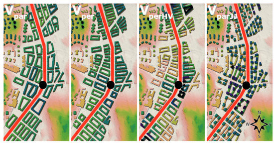
Figure 1.
The city-block-design alternatives. From left to right: V (the longer sides of buildings parallel to the boulevard), V (the longer sides perpendicular to the boulevard), V (similar to V but the building height varies) and V (similar to V but with Jing-Jang building structure variation). The boulevard is marked in red and the major junction with a black dot.

Table 2.
The specific characteristics of different city-block-design alternatives.
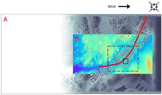
Figure 2.
The computational domain for southwesterly ( = 225) inflow conditions and V where the longer sides of building blocks are parallel to the boulevard. The domain is separated into child (B) and parent (A) domains, where the white colour stands for the topography elevation Z = 0 m. The data output domains are marked with rectangles: the small domain with a solid black and the large domain with a black dashed line. The boulevard is marked in red.
The dimensions of the parent domain are 4096 m × 2048 m × 384 m in the x-, y- and z-directions. Inside, a child domain of 2048 m × 1024 m × 96 m (Figure 2) or 1536 m × 1536 m × 96 m (not shown) for southwesterly or easterly inflow conditions, respectively, is defined. The grid spacing in all directions (x, y, z) is 1.0 m in the child and 2.0 m in the parent domain.
2.2.2. Urban Surface Data
The information on the surface elevation and cover for each x,y-pixel is fed to the model as two-dimensional ASCII-formatted raster files, with separate files for the topography (Figure 2) and tree canopy (Figure 3). The topography data contains topography elevation Z (m) above sea level (a.s.l.) and solid flow obstacles that have a volume of at least one grid box, i.e., buildings but not vehicles. Correspondingly, the tree canopy data contains the tree canopy height a.s.l. No overhanging structures are accepted in the current model version.
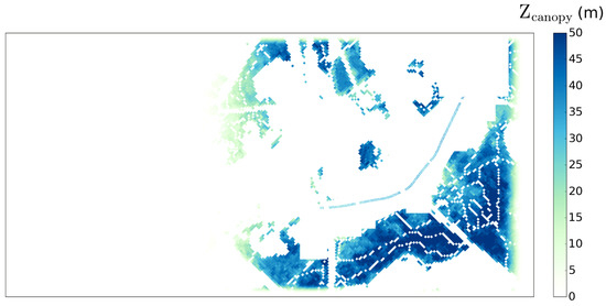
Figure 3.
A map of the tree canopy height (m) for the whole computational domain. Orientation as in Figure 2.
The landform information is obtained from the archive of the National Land Survey of Finland with a grid resolution of 2 m and the mean forest height from the archive of the Natural Resources Institute of Finland with a grid resolution of 20 m. All the rest, including the existing buildings, planned city-blocks and their corresponding street network alternatives, modifications in the landform and height of the street trees to be planted, is provided by the City Planning Department of Helsinki. Topography and building information, and mean forest and street tree heights, are superimposed on a single raster map file, respectively, which is then pivoted according to the prevailing geostrophic wind direction in each simulation. Over the whole computational domain, Z is given in a vertical resolution of 2 m. The non-cyclic inflow condition applied in the simulation (see Table 1) requires a topography-free zone of around 1.4 km in width, starting from the inflow boundary, for turbulence recycling. In addition, buffer regions of 20 m and 80 m in width, where Z is smoothed towards 20 m and 35 m (see boundaries in Figure 2), are added at the outflow and remaining lateral boundaries, respectively. This is done in order to avoid computational instabilities and to satisfy the periodic boundary conditions at the lateral boundaries [45].
2.2.3. Tree Canopy Model
The tree canopy includes two rows of planted street trees in the middle of the boulevard and the surrounding forested areas (Figure 3). At each surface x,y-grid box with vegetation, a vertical profile of the plant area density () is defined (Figure 4). Street trees are modelled as 20-m-tall Tilia × vulgaris trees, for which the vertical profile is constructed based on an experimental 5-year mean summertime value of the leaf area density = 5.3 m m for Tilia × vulgaris trees in Viikki, Helsinki [46]. In addition to leaf area, considers also the trunk and stems. The trees are assumed to have a circular cone shape with the maximum at the height of the lowest branches at 6.5 m and a surface value of 0.3 m m. Furthermore, the winter-time leaf-off period (see Section 2.3) is considered by decreasing by 80% following previous studies (e.g., [47,48]). Here, the main interest is on the impact of the street trees along the boulevard. Thus, the profiles of the trees outside the boulevard are constructed based on their height relative to the street trees. In all simulations, a drag coefficient = 0.2 is assigned following previous LES studies considering ABL flows individual trees (e.g., [41]) and forest canopies (e.g., [38,49]).
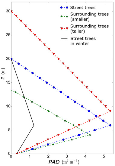
Figure 4.
The vertical profile of (m m) for the street along the boulevard (blue dashed line with dots). Example profiles for smaller and taller trees outside of the boulevard plotted in green (dashed line with stars) and red (dashed line with triangles), respectively. Additionally, the winter time profile for the street trees is given in black (solid line).
2.2.4. Lagrangian Stochastic Particle Model (LPM)
Equal to the surface cover information, the horizontal location and group of particle sources are given to LPM as a x,y-pixel raster file. The planned street network in the vicinity of the boulevard is defined as the particle source area (Figure 5). Hence, only the local traffic emissions are taken into account similar to previous numerical ventilation studies (e.g., [50]). This assumption is adequate enough since ventilation depends on the short-term temporal variation of the concentration of a substance, which is mainly governed by local sources.

Figure 5.
The particle source area (in colours) in the block-design alternatives V and V. Source areas are divided into groups 1, 2 and 3 based on the estimated mean traffic rates in year 2025 (see legends). Street surfaces below trees (white dots) are omitted as source areas. Orientation as in Figure 2.
Particles are released at a constant rate of 0.25 m s within each 1 m × 1 m × 1 m source grid box. No particles are released below the street trees. The street network is divided into three particle groups (i = 1–3) according to the estimated traffic rates in year 2025 provided by the City Planning Department of Helsinki (Figure 5). Group 1 covers minor side streets with less than 3000 vehicles per day, group 2 medium streets with 3000 to 10,000 vehicles per day and group 3 the boulevard itself and a major crossroads with over 10,000 vehicles per day. To take into account the proportional difference of traffic rates, (see Equation (1)) is calculated by defining for each particle group. In order to remove the particles stuck in the computational domain and unnecessarily increasing the computational load, their maximum age is set to 800 s, after which particles disappear from the domain. This is a loosely calculated expected time for a particle to travel across the child domain with a speed of 2 m s.
LPM is applied only inside the child domain (Figure 2). Particles are restrained from entering the parent domain by setting an absorption condition at all boundaries, except at the bottom where particles are reflected. Detailed information about LPM can be found in [51].
2.3. Computational Set-Up
The different boundary conditions used for the parent and child domains are listed in Table 1. The roughness length applied in the wall treatment using MOST is set to 0.05 m at all solid surfaces. A sufficiently developed turbulent inflow, with which the main runs are initialised, is created with a precursor runs. The characteristics of the inflow, including u, and Reynolds stress , are illustrated in Figure 6. The ABL depth is set in the precursor run by imposing a large vertical gradient to the potential temperature , i.e., a strong temperature inversion, from the ABL height up to the total height of the computational domain. This inversion prevents the ABL from increasing with time.
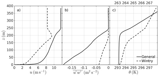
Figure 6.
The vertical profile of (a) streamwise velocity u (m s), (b) Reynolds stress (m s), and (c) potential temperature (K) at the inflow boundary for the general (solid line) and wintry (dashed line) inflow conditions. The top x-axis for is for the wintry conditions.
In order to examine the influence of the meteorological conditions of the inflow on pollutant dispersion and ventilation, two contrasting conditions are employed in the simulations. The first runs are conducted applying “general” meteorological conditions in Helsinki with a neutrally stratified ABL of 200 m in height and a geostrophic wind of m s from the southwest () [52]. The surface heat flux is set to zero to maintain the neutral atmospheric stability. Densely built urban areas tend to be unstably stratified in Helsinki (e.g., [53,54]), and thus applying a neutral stability is a conservative choice as the removal of air pollutants by turbulence is found to improve under unstable conditions [55,56]. The second runs are performed applying “wintry” meteorological conditions with a moderately stable ABL of around 160 m in height and a geostrophic wind of m s from the east (). This simulates conditions that usually lead to worst air quality events in Helsinki in winter if the Siberian high is prevailing. The atmospheric stability and vertical wind profile applied are follow those in Basu and Porté-Agel [57], and they are attained by initializing the precursor run with these profiles and applying a surface heat exchange rate of K m s to maintain the atmospheric stability. Simulating a stably stratified ABL is a challenging task as turbulent eddies are small, and a relatively high grid resolution is needed in order to resolve most of the energy containing turbulence [39]. Furthermore, two supportive simulations were conducted for all design versions: under a neutral stratification but with an easterly wind, and under stable stratification but with a southwesterly wind. Results of the simulations are shown in Appendix B, Appendix D and Appendix E.
2.4. Simulations and Data Output
Complete simulations are done in several parts. First, one precursor run per each inflow condition is carried out over one hour (3600 s) and the final state of the run is applied to initialize the main runs. The main run is carried out in batches of 55 min (batch 1) and 6 min (batch 2). The second batch starts from the final state of the first batch. The release of particles starts after 5 min from the start of batch 1 and is stopped at 56 min, i.e., one minute after the start of batch 2.
Data are output in three sequences over two different domains of 0.5 km and 0.04 km (Figure 2) after the transients formed in the initialisation of the main run have subdued. Data output 1 with a time interval of 5 s is collected over the large data output domain over a time span of 40 min starting at 15 min. The high frequency data output 2 starts after 50 min with an interval equal to the integration time step of the simulation of ca. 0.07 s and 0.15 s under the neutrally and stably stratified inflow, respectively. Due to the high logging frequency, the data output 2 covers only the small data output domain. The data output 3 is collected over the large data output domain at a time interval of 5 s during the last 5 min of the simulation when the release of particles has been stopped. The vertical resolution is 1.0 m for all data output whereas the horizontal resolution is 1.0 m for the data output 2 and 2.0 m for the outputs 1 and 3.
2.5. Ventilation and Dispersion Measures
Ventilation and dispersion of pollutants in street canyons and courtyards is assessed by three different measures: number concentration (m), which from hereafter equals for the sake of simplicity, the vertical turbulent flux density (m s) and dilution rate D (m s) of particles. Various other measures have also been proposed in the literature, for instance the exchange velocity [58], the local purging flow rate and visitation frequency [59], the mean tracer age and age distribution [60], the net escape velocity [61], and the particle exchange rate which assumes horizontal homogeneity of [50]. These measures are however applicable only for simplified urban areas. The velocity ratio [34], on the other hand, does not directly measure pollutant ventilation, and therefore is not used here.
is calculated as the covariance between the vertical wind velocity and the particle number concentration as follows:
where and are the instantaneous fluctuating vertical velocity and particle number concentration at point () at time t, and the overbar denotes the time average over a selected averaging period. Before calculating the covariance, linear de-trending is applied on both time series. Positive indicates upward transport, i.e., ventilation, and negative downward, i.e., re-entrainment of particles from air above. Hence, the higher the higher ventilation. has previously been observed to determine pollutant removal from street canyons in CFD studies over idealized street canyons (e.g., [15,17,62,63,64]) as well as in wind tunnel simulations (e.g., [65]). By contrast, advective flux densities are shown to govern the redistribution of pollutants below the roof level [17]. Therefore, to study pollutant ventilation, only the turbulent transport is examined here. is calculated at z = 20 m, which is the minimum roof height of all city-block-design versions and well above the surface. Furthermore, is calculated both from the high frequency data output 2 () and the low frequency data output 1 (). As regards the low temporal frequency of 0.2 Hz of the data output 1, a proportion of the total may be missed and thus the exact values of should be treated with caution. On the other hand, representativeness of calculated only over the small data output domain is limited. Therefore, is compared to over the same domain in order to show the applicability of in this comparative study.
Particle dilution rate D is calculated after the particle source has been switched of at 56 min in batch 2 as
where is the output time step. The higher D, the higher ventilation. According to the scalar conservation equation (e.g., Equation (5) in [35]), D equals to the sum of the advective and turbulent transport terms if no sources are present. D is calculated from the data output 3 inside an air volume below 20 m a.g.l. First, to minimize the dependence of D on the initial particle concentration, the initial total particle concentration values (t = 0) inside the analysis domain in each block-design version are normalized relative to that of design version V. The analysis of D is based on two measures: volume average over a volume of 0.015 km (around 2.4 million grid cells) and time-column average within each 2 m × 2 m × 20 m vertical column. The dilution of particles is observed to occur very rapidly as the total particle concentrations drop to half within 60–120 s. Hence, only the first 50 s of the data output 3 are selected for the analysis, which is also the averaging period for . Sensitivity of to the averaging period was tested by altering the averaging period by ±20 s (see Appendix F).
3. Results
From hereafter, all heights are given in heights above ground level (a.g.l.) unless otherwise specified. The major junction refers to the junction marked in Figure 1. Along with spatial visualisation, the different measures (, and D) are analysed separately over the boulevard (marked in Figure 1), other street canyons excluding the boulevard, courtyards, and surroundings, which is the surface area classified neither as a street canyon nor a courtyard, covering around 50% of the large data output domain.
3.1. Particle Concentration pc
The 40-min temporal mean and 90th percentile values of are calculated for two layers, z = 3–5 m and z = 9–11 m, in both inflow conditions. The mean values for both heights separated to the areas defined above are shown in Figure 7, and the horizontal distributions at z = 4 m are displayed in Figure 8. The mean distributions at z = 10 m and 90th percentiles at both heights follow closely the mean values at z = 4 m, which is hence considered to represent the horizontal variation of .
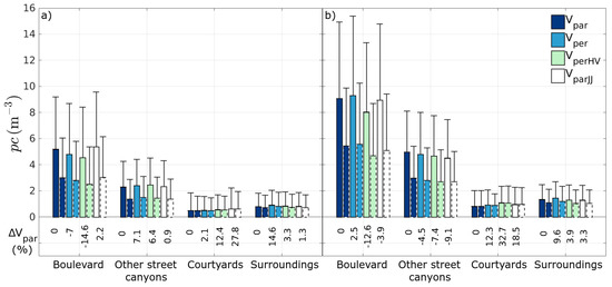
Figure 7.
40-min horizontal mean particle concentrations (m) under the (a) general and (b) wintry inflow conditions separately above the boulevard, other street canyons, courtyards and surroundings at height z = 4 m (bars with solid lines) and z = 10 m (bar with dashed lines) for all runs. 90th percentile values are given with errorbars. The mean difference to the values in V is given in percentages (V).
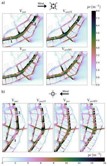
Figure 8.
40-min temporal mean of particle concentration (m) at height z = 4 m under the (a) general and (b) wintry inflow conditions. Notice the orientation of the mean wind and different scales of . Cross sections in Figure 8 are marked with white lines.
In general, the spatial variability of within the study domain is notable with higher values along the boulevard than in other areas. Under the general inflow conditions (Figure 8a), the concentration patterns in the southern and northern parts of the boulevard are distinctly different, as the mean wind direction relative to the boulevard changes from nearly parallel to oblique, respectively. The perpendicular wind component results in accumulation to the upwind side of the boulevard due to particle transport by canyon vortex circulation (e.g., [15]). This accumulation is however weak in V. Even though the largest concentrations are commonly seen at the boulevard, some strong accumulation is formed along the side street west of the major junction. Accumulation here is particularly notable in V with building height decreasing downwind, which is attributable to a typically weaker canyon vortex inside this type of step-down canyons (e.g., [65]). In the northern part, the hotspots of on the leeward side of the boulevard are nearly continuous along the boulevard in V and V, whereas in V and V ventilation from the cross streets breaks the accumulation patterns.
Under the wintry inflow conditions (Figure 8b), the mean wind direction is close to perpendicular to the boulevard, especially north of the major junction. A large forested area lies to the east of the boulevard, and hence its cross streets provide fresh, unpolluted air and decrease the mean concentrations along those streets and the boulevard. This is particularly emphasised in V and V which have more cross streets. In the southern part of the boulevard, the smallest particle accumulation on the leeward side of the boulevard is seen in V. Yet, north of the major junction are not distinctly higher in V than in V despite building height decreasing downwind in V in this wind direction, which is generally expected to weaken the canyon vortex and ventilation (e.g., [65]).
Notwithstanding the lower values of street trees in the simulations under the wintry inflow conditions, at z = 4 m are approximately two-fold compared to the general inflow conditions, which demonstrates how strongly meteorology influences pollutant dispersion. Under both inflow conditions, values are of the same magnitude in V and V. The courtyards are notably clean and remains low throughout all simulations.
The vertical dispersion of and mean flow structure inside the boulevard street canyon for two vertical cross Section 1 and Section 2 marked in Figure 8 are shown in Figure 9a,b under the general, and Figure 9c,d under the wintry inflow conditions. In Figure 9a (cross Section 1), the wind is close to parallel to the canyon, i.e., towards the picture, and due to flow channelling and advective particle transport the concentrations remain low. In Figure 9b (cross Section 2), instead, the mean wind has a strong perpendicular component creating optimal conditions for a canyon vortex. However, the street trees block the flow and break the vortex in two. This explains the more consistent dispersion of inside the canyon and accumulation on both sides of the boulevard. Under the wintry inflow conditions, on the other hand, a uniform canyon vortex is formed, and it is emphasised in V and V with longer street canyons along the boulevard. Yet the exact location varies between the city-block versions. Vertical maxima of under both inflow conditions are seen right below the maximum of the profile at z = 6.5 m.
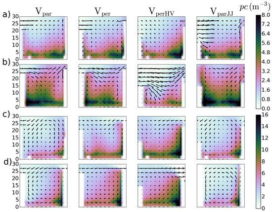
Figure 9.
40-min mean particle concentration (m) across the boulevard. (Cross Section 1 and Section 2, which are marked in Figure 8, are shown in (a,b) under the general inflow conditions, and in (c,d) under the wintry inflow conditions, respectively. Cross sections are viewed from the south. Lengths of the wind arrows are relative to the wind speeds normal to the cross section. Height in m a.g.l. are given in the left. Notice the different scales of .)
In spite of the great spatial variability in between the block-design versions, the concentration characteristics of different block-design versions are similar at both 4 and 10 m levels in almost all cases, as shown in Figure 7. Above the boulevard, both the mean values and 90th percentiles are lowest in V under both general and wintry inflow conditions, whereas the highest values are observed in V and V under the general and wintry inflow conditions, respectively. In other street canyons, no systematic pattern is seen while in the courtyards and surroundings, V has on average the lowest mean concentrations.
3.2. Turbulent Particle Flux
Due to data constrains, was computed only for the small data output domain, which is visualised Appendix C. Furthermore, the lower resolution was also calculated in order to compare the turbulent particle flux with the other metrics used in the study. To estimate possible uncertainties originating from the lower temporal resolution, Table 3 summarizes the mean values of both and in the same small data output domain separately for the boulevard, other street canyons, courtyards and surroundings. Overall, and show rather similar orders of magnitude between the design-versions except above the boulevard under the general inflow conditions and in the surroundings under the wintry inflow conditions. generally overestimates flux density values, apart from above the courtyards and above the other street canyons under the general inflow conditions. However, a Student’s one-sample t-test for the difference of the values of and shows that the difference is insignificant at 95% confidence level (p = 0.069). and values agree better under the wintry than the general inflow conditions, owing most likely to the nearly three times longer time step of the wintry simulations. The difference between and becomes even less significant (p = 0.18), if under the general inflow conditions is calculated using only every other time step of the data output 2 when the data logging frequency is around 7 Hz. As a conclusion, can be applied when comparing ventilation in different city-block-design versions.

Table 3.
Horizontal mean of the high-frequency vertical turbulent particle flux density (m s) separately for the boulevard, other street canyons, courtyards and surroundings at z = 20 m under both general and wintry inflow conditions. Horizontal mean of the low-frequency vertical turbulent particle flux density over the same domain is given in brackets.
The horizontal distribution and mean values of above the separate areas for all block-design versions under both inflow conditions are visualised in Figure 10 and Figure 11. For all model runs, appears to be on average positive indicating upward transport of particles and ventilation. This can be expected since the particle source is constantly maintaining at street level. In general, inside the courtyards is close to zero or even negative, as the only sources are re-entrainment from above or advection from the building openings. is slightly increased when the building height increases and correspondingly decreased when the building height decreases downwind in V. Furthermore, values are smaller under the wintry than the general inflow conditions. Under the general inflow conditions, shows most positive values along the boulevard in V, whereas in the other design versions areas of negative flux density (re-entrainment) also appear. Under the wintry inflow conditions, is most positive in V and V. In V, a vast area of negative flux density is observed south of the major junction. The same is observed in V as well but less pronounced. is decreased on the leeward side of buildings and especially behind the corners of buildings and higher towers in V, which is reflected to particle concentrations.
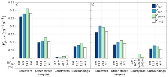
Figure 10.
Horizontal mean of the low-frequency vertical turbulent particle flux density (m s) under the (a) general and (b) wintry inflow conditions separately for the boulevard, other street canyons, courtyards and surroundings at z = 20 m for all runs. The difference to the value in V is given in percentages (V).
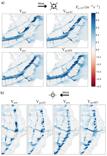
Figure 11.
40-min mean low-frequency vertical turbulent particle flux density (m s) at z = 20 m under the (a) general and (b) wintry inflow conditions. Positive values indicate upward flux.
Horizontal mean values in Figure 10 correspond well to the visual analysis based on Figure 11. As noted, values are higher under the general inflow conditions. is mainly largest in V and smallest in V under both inflow conditions. Both V and V show higher values than V regardless of weather conditions. Furthermore, over the courtyards in V depends strongly on the inflow.
3.3. Particle Dilution Rate D
The time series of under the general (a) and wintry (b) inflow conditions are illustrated in Figure 12. Values are given relative to in V. Overall, shows high variability with time notwithstanding the spatial averaging of D over around 2.4 million grid points. Figure 12a for the general inflow conditions reveals no significant differences between V, V and V whereas they all show mostly smaller values than V. Under the wintry inflow conditions (Figure 12b), in V and particularly in V remain mostly above that in V whereas in V varies between above and below.
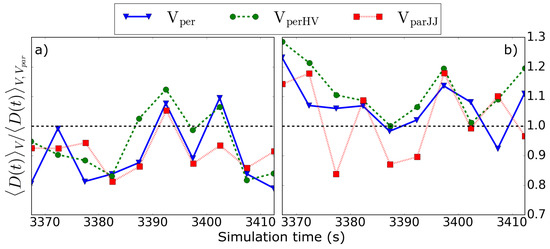
Figure 12.
The volume averaged particle dilution rate (m s) between z = 1–20 m under the (a) general and (b) wintry inflow conditions. Results are represented relative to V ().
The horizontal distribution and mean values of above the boulevard, other street canyons, courtyards and surroundings under both inflow conditions are displayed in Figure 13 and Figure 14. The analysis area is the same as for and . In general, increases downwind under both general and wintry inflow conditions as particles in the upwind columns are transported quickly by the horizontal advection. Furthermore, values are twofold under the wintry compared to the general inflow conditions. This also shown in the supportive simulations in Appendix E. Especially V shows efficient dilution to the surroundings. Sensitivity tests show how the averaging period over which is calculated has minor impact on the results (Appendix F).
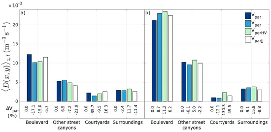
Figure 13.
Mean (×10 m s) under the (a) general and (b) wintry inflow conditions separately for the boulevard, other street canyons, courtyards and surroundings between z = 1–20 m for all runs. D is calculated using data from the first 50 s after the particle source has been switched off. The difference to the value in V is given in percentages (V).
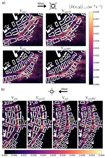
Figure 14.
The temporal mean particle dilution rate (m s) between z = 1–20 m for the first 60 s after the particle has been switched off: (a) general and (b) wintry inflow conditions.
Horizontal mean values in Figure 14 quantify the differences in between the design versions. Along the boulevard, dilution is most efficient in V and V under the general inflow conditions, and in V under the wintry inflow conditions. The efficient dilution to the surroundings in V is seen also in the mean values, especially in the wintry inflow conditions. Moreover, V shows mostly higher values than V. Dilution inside the courtyards is weakest in V.
4. Discussion
Pollutant dispersion is strongly governed by inflow conditions: wind parallel to a street canyon sweeps the particles away due to particle transport by horizontal advection, as also shown by Moon et al. [66], whereas perpendicular or oblique winds result in accumulation to the leeward side. Mean concentrations are two-fold under the wintry compared to the general inflow conditions, which stems from less efficient vertical mixing and pollutant transport in stable ABL (see also Appendix B). On the other hand, Figure 10 and Appendix D show that vertical transport is notably higher under a southwesterly wind despite the atmospheric stability. This is likely due to more efficient mechanical production of turbulence under a southwesterly wind as the inflow travels over a longer stretch of urban area before entering the area of interest, unlikely when the wind is from the east with mostly homogeneous vegetated areas.
Urban morphology is shown to have a significant role in the dispersion of particles, which is illustrated in Figure 7 and Figure 8. Greatest concentrations along the boulevard and weakest vertical transport are observed when the longer sides of building blocks are parallel to the boulevard, which supports previous studies performed over idealised street canyons [63,67,68]. Non-uniform building height in V is shown to decrease accumulation on the leeward side of the boulevard street canyon, especially under a southwesterly wind when the building height mainly increases downwind [65,69,70]. Apart from buildings, street trees can alter the flow field and canyon vortex, and thereby decrease pollutant ventilation. Therefore, a detailed representation of trees in urban flow and air quality simulations is of high importance.
Of all the design options, V with building height variation results on average in the greatest ventilation rates and lowest street level concentrations above the street canyons, with around 7–9% lower concentrations at z = 4 m than the city-block-design alternative with highest concentrations inside street canyons. The result supports previous studies conducted over simplified urban topographies (e.g., [60,65,71,72,73,74]). The building shape variability in V, instead, is mainly shown to increase and improve ventilation in vertical, whereas the mean values of and D display equally efficient or even weaker ventilation than in V. The result indicates that the aerodynamically rougher city-blocks in V do not notably improve the air quality near the pedestrian level. The irregularities in the building shape in V probably destroy the canyon vortex [75], which reduces advective particle transport. Further in–depth studies are needed to explain the last-mentioned result.
Applying a high-resolution LES model over a real urban topography of a vast extent provides a large amount of detailed information about the flow and concentration fields. However, the amount of output data is high and the complexity of the topography further complicates the analysis. The ventilation measures chosen to be applied in this study cover the pollutant dispersion mechanisms broadly and complement each other. Based on the results, the following generalisation can be deduced. The pedestrian level concentrations are lowest when are highest. Furthermore, under both inflow conditions the highest mean values of are observed in the V and lowest in V, suggesting that is strongly determined by the urban morphology. Generally, D is correlated to , and the differences between their horizontal distributions stem from the flow changing the location of particles but not necessarily removing them from the study domain. A comparison of the horizontal patterns of and points out areas where the dilution in vertical is notable and vice versa. On the whole, however, the patterns are unlike, indicating that D measures mainly horizontal advection. This advective nature of D can also be concluded from the higher values when the flow is parallel to the longer sides of buildings as the flow is horizontally less blocked and disturbed by flow structures created by building corners. Last of all, as well as and D are smaller in courtyards and surroundings than inside street canyons indicating little particle transport from the streets. The vertical exchange above courtyards is shown to be low when the angle between the wind and principal courtyard axis is around 90, supporting results by Moonen et al. [76].
Owing to the large extent of the study domain, the analysis was confined to the temporal mean values of the analysis measures. Moreover, the number of different inflow conditions applied was limited to two due to the high computational expenses of the simulations. They were, however, carefully chosen to represent typical and worst-case conditions at the modelling site, but also for the results to apply as guidelines in all urban areas. Last of all, the study focused on the aerodynamic impacts and omitted, for instance, air pollutant chemistry and dynamics and anthropogenic heat sources.
Explicit rules can be difficult to give to optimize of flow and pollutant dispersion over complex urban terrains [71]. To yield detailed information for a specific case, similar studies have to be conducted separately for each urban planning solution. However, the outcome of this study, related firstly to the most efficient dispersion in V with variable building height and short wall facing the main road and secondly to the insignificant improvement of ventilation by building shape variation in V, can be used as a general guideline also for other areas. Such information is vital for urban planners in order to design dense urban areas where the level of pollution exposure is minimized. For decision making, a separate model could be used in which each of the ventilation measures and areas of interest would get a weighting factor. Based on the factors that are considered important, for instance good ventilation inside courtyards, one could define the most suitable city-block-design alternative.
5. Conclusions
This study examines how the structural arrangement and orientation of perimeter blocks affect the ventilation and dispersion of traffic-related emissions within their street canyons under two contrasting meteorological conditions of the inflow. The principal objective of this numerical study is to demonstrate means to generate information that enables future urban planners to improve the pedestrian level air quality within real urban areas. The study is comprised of simulations that feature four different virtual building-block arrangements that are proposed for a real city boulevard site. In addition to buildings, the representation of the urban area is highly realistic including surrounding landform as well as forested areas and street trees. The simulations are conducted using a LES model PALM with an embedded Lagrangian stochastic particle model. The Lagrangian particles representing massless and inert air pollutant tracers are released over streets with a source strength (i.e., weighted particle release rate) that is relative to the local traffic volumes. The study employs a full three-dimensional two-way self-nesting functionality, which is newly implemented to PALM.
The analysis is founded on three different measures: particle concentration , vertical turbulent particle transport and particle dilution rate D. Variation in building height is shown to enhance both and D, and thus decrease accumulation of at pedestrian level. Furthermore, short canyons by the boulevard are shown preferential for . However, building shape variability of smaller scale does not result in improved ventilation. D is governed by horizontal advection and is thus strongly determined by the horizontal wind direction. It is shown how the design version with the shortest wall parallel to the boulevard with variable building height creates on average the most optimal air quality at pedestrian level along the boulevard, but the spatial variability within the street is highly variable depending on the pollutant transport and dispersion. Courtyards remain clean throughout all simulations, implying that in general traffic-related pollutants are not easily transported to there. Despite the high roughness and complexity of the urban surface that leads to efficient mechanical production of turbulent, pollutant concentrations are clearly higher under stably stratified inflow conditions.
This is the first LES study over a vast, urban area applying sophisticated measures to assess pollutant dispersion and ventilation. The numerical methods are novel and highly developed providing realistic estimations for the removal of nonreactive gaseous air pollutants from the pedestrian level. The results of this study provide unique information about the transport of traffic-related pollutants in this specific urban environment and the results can directly be applied by local urban planners, but naturally the findings support urban planning also in other cities.
Supplementary Materials
The modified code parts of PALM revision 1904 used in this study are available online at http://www.mdpi.com/2073-4433/9/2/65/s1.
Acknowledgments
This study was commissioned and funded by the City Planning Department (current Urban Environment Division) of the City of Helsinki. We also acknowledge the Doctoral Programme in Atmospheric Sciences (ATM-DP, University of Helsinki), Helsinki Metropolitan Region Urban Research Program and the Academy of Finland (181255, 277664) for financial support.
Author Contributions
M.K. constructed the model set-up, carried out the simulations, analysed the data and wrote the manuscript; A.H. and M.A. planned the experiments together with M.K., supervised her in performing the simulations and analysing the data, and commented on the manuscript; S.R. and T.V. provided critical feedback on the manuscript and helped shape the research; L.J. supervised the project and took actively part in writing the manuscript.
Conflicts of Interest
The authors declare no conflict of interest. The founding sponsors had no role in the design of the study; in the collection, analyses, or interpretation of data; in the writing of the manuscript, and in the decision to publish the results.
Abbreviations
The following abbreviations are used in this manuscript:
| ABL | Atmospheric boundary layer |
| CFD | Computational fluid dynamics |
| LAD | Leaf area density |
| LES | Large-eddy simulaion |
| LPM | Lagrangian stochastic particle model |
| MOST | Monin-Obukhov similarity theory |
| PAD | Plant area density |
| PALM | Parallelized Large-Eddy Simulation Model |
| par | parallel |
| parJJ | paraller with Jin-Jang shape variation |
| per | perpendicular |
| perHV | perpendicular with height variation |
| RANS | Reynolds-averaged Navier-Stokes equations |
Appendix A. Technical Specifications

Table A1.
Technical specifications for the simulations conducted with the LES model PALM.
Table A1.
Technical specifications for the simulations conducted with the LES model PALM.
| V | Characteristics |
|---|---|
| Programming language | Fortran 95/2003 |
| Discretization | Arakawa staggered C-grid [77,78] |
| Parallelization | Two-dimensional domain decomposition (e.g., [36]). Communication between processors realized using Message Passing Interface (MPI). |
| Sub-grid closure | 1.5-order scheme based on Deardorff [79] |
| Advection scheme | 5th-order advection scheme by Wicker and Skamarock [80] |
| Pressure solver | Iterative multigrid scheme (e.g., [81]) |
| Time step closure | 3rd-order Runge-Kutta approximation [82] |
| Boundary condition between the surface and the first grid level | Monin-Obukhov similarity theory [83] |
Appendix B. Particle Concentration pc for the Supportive Simulations
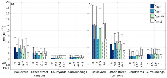
Figure A1.
40-min horizontal mean particle concentrations () for the (a) neutral run with an easterly wind and (b) stable run with a southwesterly wind separately above the boulevard, other street canyons, courtyards and surroundings at height z = 4 m (bars with solid lines) and z = 10 m (bar with dashed lines) for all runs. 90th percentile values are given with errorbars. The mean difference to the values in V is given in percentages (V).
Appendix C. 5-Minute Mean High-Frequency Vertical Turbulent Particle Flux Density Fp,HF

Figure A2.
5-min mean high-frequency vertical turbulent particle flux density (m−2 s−1) at z = 20 m under the (a) general and (b) wintry inflow conditions. The analysis area is marked in Figure 2 with a black solid line.
Appendix D. Low-Frequency Vertical Turbulent Particle Flux Density Fp,HF for the Supportive Simulations

Figure A3.
Horizontal mean of the low-frequency vertical turbulent particle flux density (m−2 s−1) for the (a) neutral and (b) stable runs separately for the boulevard, other street canyons, courtyards and surroundings at z = 20 m for all runs. The difference to the value in V is given in percentages (V).
Appendix E. Column-Averaged Dilution Rate ⟨D(x,y)⟩t,z for the Supportive Simulations

Figure A4.
Mean (×10−3 m−3 s−1) for the (a) neutral run with an easterly wind and (b) stable run with a southwesterly wind separately for the boulevard, other street canyons, courtyards and surroundings between z = 1–20 m for all runs. D is calculated using data from the first 50 s after the particle source has been switched off. The difference to the value in V is given in percentages (V).
Appendix F. Column-Averaged Dilution Rate ⟨D(x,y)⟩t,z with Different Averaging Periods

Figure A5.
Mean (×10−3 m−3 s−1) under the general (left) and wintry (right) inflow conditions separately for the boulevard, other street canyons, courtyards and surroundings between z = 1–20 m for all runs. D is calculated for different averaging periods: (a) 30 s; (b) 40 s; (c) 50 s; (d) 60 s and (e) 70 s. The difference to the value in V is given in percentages (V).
References
- United Nations. World Urbanization Prospects: The 2014 Revision, Highlights; Department of Economic and Social Affairs, Population Division: New York, NY, USA, 2014. [Google Scholar]
- Brunekreef, B.; Holgate, S.T. Air pollution and health. Lancet 2002, 360, 1233–1242. [Google Scholar] [CrossRef]
- Pope, C.A.I.; Dockery, D.W. Health effects of fine particulate air pollution: Lines that connect. J. Air Waste Manag. Assoc. 2006, 56, 709–742. [Google Scholar] [CrossRef] [PubMed]
- Gakibou, E.; Afshin, A.; Abajobir, A.A.; Abate, K.H.; Abbafati, C.; Abbas, K.M.; Abd-Allah, F.; Abdulle, A.M.; Abera, S.F.; Aboyans, V.; et al. Global, regional, and national comparative risk assessment of 84 behavioural, environmental and occupational, and metabolic risks or clusters of risks, 1990–2016: A systematic analysis for the Global Burden of Disease Study 2016. Lancet 2017, 390, 1345–1422. [Google Scholar] [CrossRef]
- European Environmental Agency. Air Quality in Europe—2017 Report; EEA Report No 13/2017; Publications Office of the European Union: Luxembourg, 2017. [Google Scholar]
- Fenger, J. Air pollution in the last 50 years–From local to global. Atmos. Environ. 2009, 43, 13–22. [Google Scholar] [CrossRef]
- Vardoulakis, S.; Fisher, B.E.; Pericleous, K.; Gonzalez-Flesca, N. Modelling air quality in street canyons: A review. Atmos. Environ. 2003, 37, 155–182. [Google Scholar] [CrossRef]
- Britter, R.E.; Hanna, S.R. Flow and dispersion in urban areas. Ann. Rev. Fluid Mech. 2003, 35, 469–496. [Google Scholar] [CrossRef]
- Buccolieri, R.; Sandberg, M.; Sabatino, S.D. City breathability and its link to pollutant concentration distribution within urban-like geometries. Atmos. Environ. 2010, 44, 1894–1903. [Google Scholar] [CrossRef]
- Tominaga, Y.; Stathopoulos, T. Ten questions concerning modeling of near-field pollutant dispersion in the built environment. Build. Environ. 2016, 105, 390–402. [Google Scholar] [CrossRef]
- Giometto, M.G.; Christen, A.; Meneveau, C.; Fang, J.; Krafczyk, M.; Parlange, M.B. Spatial Characteristics of Roughness Sublayer Mean Flow and Turbulence over a Realistic Urban Surface. Bound. Layer Meteorol. 2016, 160, 425–452. [Google Scholar] [CrossRef]
- Gousseau, P.; Blocken, B.; Stathopoulos, T.; van Heijst, G. CFD simulation of near-field pollutant dispersion on a high-resolution grid: A case study by LES and RANS for a building group in downtown Montreal. Atmos. Environ. 2011, 45, 428–438. [Google Scholar] [CrossRef]
- Tominaga, Y.; Stathopoulos, T. CFD modeling of pollution dispersion in a street canyon: Comparison between LES and RANS. J. Wind Eng. Ind. Aerodyn. 2011, 99, 340–348. [Google Scholar] [CrossRef]
- Salim, S.M.; Cheah, S.C.; Chan, A. Numerical simulation of dispersion in urban street canyons with avenue-like tree plantings: Comparison between RANS and LES. Build. Environ. 2011, 46, 1735–1746. [Google Scholar] [CrossRef]
- Baik, J.J.; Kim, J.J. On the escape of pollutants from urban street canyons. Atmos. Environ. 2002, 36, 527–536. [Google Scholar] [CrossRef]
- Cai, X.M.; Barlow, J.; Belcher, S. Dispersion and transfer of passive scalars in and above street canyons—Large-eddy simulations. Atmos. Environ. 2008, 42, 5885–5895. [Google Scholar] [CrossRef]
- Li, X.X.; Liu, C.H.; Leung, D.Y. Numerical investigation of pollutant transport characteristics inside deep urban street canyons. Atmos. Environ. 2009, 43, 2410–2418. [Google Scholar] [CrossRef]
- Raupach, M.R.; Finnigan, J.J.; Brunet, Y. Boundary-Layer Meteorology 25th Anniversary Volume, 1970–1995: Invited Reviews and Selected Contributions to Recognise Ted Munn’s Contribution as Editor over the Past 25 Years; Chapter Coherent Eddies and Turbulence in Vegetation Canopies: The Mixing-Layer Analogy; Springer: Dordrecht, The Netherlands, 1996; pp. 351–382. [Google Scholar]
- Gromke, C.; Blocken, B. Influence of avenue-trees on air quality at the urban neighborhood scale. Part II: Traffic pollutant concentrations at pedestrian level. Environ. Pollut. 2015, 196, 176–184. [Google Scholar] [CrossRef] [PubMed]
- Oke, T.R. Boundary Layer Climates, 2nd ed.; Routledge: London, UK, 1987. [Google Scholar]
- Buccolieri, R.; Gromke, C.; Sabatino, S.D.; Ruck, B. Aerodynamic effects of trees on pollutant concentration in street canyons. Sci. Total Environ. 2009, 407, 5247–5256. [Google Scholar] [CrossRef] [PubMed]
- Gromke, C.; Ruck, B. On the Impact of Trees on Dispersion Processes of Traffic Emissions in Street Canyons. Bound. Layer Meteorol. 2009, 131, 19–34. [Google Scholar] [CrossRef]
- Mochida, A.; Lun, I.Y. Prediction of wind environment and thermal comfort at pedestrian level in urban area. J. Wind Eng. Ind. Aerodyn. 2008, 96, 1498–1527. [Google Scholar] [CrossRef]
- Vos, P.E.; Maiheu, B.; Vankerkom, J.; Janssen, S. Improving local air quality in cities: To tree or not to tree? Environ. Pollut. 2013, 183, 113–122. [Google Scholar] [CrossRef] [PubMed]
- Lindberg, F.; Grimmond, C.S.B. Continuous sky view factor maps from high resolution urban digital elevation models. Clim. Res. 2010, 42, 177–183. [Google Scholar] [CrossRef]
- Nordbo, A.; Karsisto, P.; Matikainen, L.; Wood, C.R.; Järvi, L. Urban surface cover determined with airborne lidar at 2 m resolution—Implications for surface energy balance modelling. Urban Clim. 2015, 13, 52–72. [Google Scholar] [CrossRef]
- Gousseau, P.; Blocken, B.; Stathopoulos, T.; van Heijst, G. Near-field pollutant dispersion in an actual urban area: Analysis of the mass transport mechanism by high-resolution Large Eddy Simulations. Comput. Fluids 2015, 114, 151–162. [Google Scholar] [CrossRef]
- Kanda, M.; Inagaki, A.; Miyamoto, T.; Gryschka, M.; Raasch, S. A New Aerodynamic Parametrization for Real Urban Surfaces. Bound. Layer Meteorol. 2013, 148, 357–377. [Google Scholar] [CrossRef]
- Letzel, M.O.; Krane, M.; Raasch, S. High resolution urban large-eddy simulation studies from street canyon to neighbourhood scale. Atmos. Environ. 2008, 42, 8770–8784. [Google Scholar] [CrossRef]
- Park, S.B.; Baik, J.J.; Lee, S.H. Impacts of Mesoscale Wind on Turbulent Flow and Ventilation in a Densely Built-up Urban Area. J. Appl. Meteorol. Climatol. 2015, 54, 811–824. [Google Scholar] [CrossRef]
- Xie, Z.T.; Castro, I.P. Large-eddy simulation for flow and dispersion in urban streets. Atmos. Environ. 2009, 43, 2174–2185. [Google Scholar] [CrossRef]
- Keck, M.; Raasch, S.; Letzel, M.O.; Ng, E. First Results of High Resoltuion Large-Eddy Simulations of the Atmospheric Boundary Layer. J. Heat Island Inst. Int. 2014, 9, 39–43. [Google Scholar]
- Cui, Z.; Cai, X.; Baker, C.J. Large-eddy simulation of turbulent flow in a street canyon. Q. J. R. Meteorol. Soc. 2004, 130, 1373–1394. [Google Scholar] [CrossRef]
- Letzel, M.O.; Helmke, C.; Ng, E.; An, X.; Lai, A.; Raasch, S. LES case study on pedestrian level ventilation in two neighbourhoods in Hong Kong. Meteorol. Z. 2012, 21, 575–589. [Google Scholar] [CrossRef]
- Maronga, B.; Gryschka, M.; Heinze, R.; Hoffmann, F.; Kanani-Sühring, F.; Keck, M.; Ketelsen, K.; Letzel, M.O.; Sühring, M.; Raasch, S. The Parallelized Large-Eddy Simulation Model (PALM) version 4.0 for atmospheric and oceanic flows: Model formulation, recent developments, and future perspectives. Geosci. Model Dev. 2015, 8, 2515–2551. [Google Scholar] [CrossRef]
- Raasch, S.; Schröter, M. PALM—A large-eddy simulation model performing on massively parallel computers. Meteorol. Z. 2001, 10, 363–372. [Google Scholar] [CrossRef]
- Hoffmann, F.; Raasch, S.; Noh, Y. Entrainment of aerosols and their activation in a shallow cumulus cloud studied with a coupled LCM–LES approach. Atmos. Res. 2015, 156, 43–57. [Google Scholar] [CrossRef]
- Kanani-Sühring, F.; Raasch, S. Spatial Variability of Scalar Concentrations and Fluxes Downstream of a Clearing-to-Forest Transition: A Large-Eddy Simulation Study. Bound. Layer Meteorol. 2015, 155, 1–27. [Google Scholar] [CrossRef]
- Beare, R.J.; Macvean, M.K.; Holtslag, A.A.M.; Cuxart, J.; Esau, I.; Golaz, J.C.; Jimenez, M.A.; Khairoutdinov, M.; Kosovic, B.; Lewellen, D.; et al. An Intercomparison of Large-Eddy Simulations of the Stable Boundary Layer. Bound. Layer Meteorol. 2006, 118, 247–272. [Google Scholar] [CrossRef]
- Razak, A.A.; Hagishima, A.; Ikegaya, N.; Tanimoto, J. Analysis of airflow over building arrays for assessment of urban wind environment. Build. Environ. 2013, 59, 56–65. [Google Scholar] [CrossRef]
- Giometto, M.G.; Christen, A.; Egli, P.E.; Schmid, M.F.; Tooke, R.T.; Coops, N.C.; Parlange, M.B. Effects of trees on mean wind, turbulence and momentum exchange within and above a real urban environment. Adv. Water Resour. 2017, 106, 154–168. [Google Scholar] [CrossRef]
- Hellsten, A.; Ketelsen, K.; Barmpas, F.; Tsegas, G.; Moussiopoulos, N.; Raasch, S. Nested multi-scale system in the PALM large-eddy simulation model. In Proceedings of the 35th International Technical Meeting on Air Pollution Modelling and its Application, Chania, Crete, Greece, 3–7 October 2016; Springer: Cham, Switzerland, 2017; pp. 287–292. [Google Scholar]
- Kataoka, H.; Mizuno, M. Numerical flow computation around aeroelastic 3D square cylinder using inflow turbulence. Wind Struct. 2002, 5, 379–392. [Google Scholar] [CrossRef]
- Zhang, X.; Shu, C.-W. On Maximum-principle-satisfying High Order Schemes for Scalar Conservation Laws. J. Comput. Phys. 2010, 229, 3091–3120. [Google Scholar] [CrossRef]
- Auvinen, M.; Järvi, L.; Hellsten, A.; Rannik, U.; Vesala, T. Numerical framework for the computation of urban flux footprints employing large-eddy simulation and Lagrangian stochastic modeling. Geosci. Model Dev. 2017, 10, 4187–4205. [Google Scholar] [CrossRef]
- Riikonen, A.; Järvi, L.; Nikinmaa, E. Environmental and crown related factors affecting street tree transpiration in Helsinki, Finland. Urban Ecosyst. 2016, 19, 1693–1715. [Google Scholar] [CrossRef]
- Groenendijk, M.; Dolman, A.J.; Ammann, C.; Arneth, A.; Cescatti, A.; Dragoni, D.; Gash, J.H.C.; Gianelle, D.; Gioli, B.; Kiely, G.; et al. Seasonal variation of photosynthetic model parameters and leaf area index from global Fluxnet eddy covariance data. J. Geophys. Res. Biogeosci. 2011, 116, G04027. [Google Scholar] [CrossRef]
- Muraoka, H.; Saigusa, N.; Nasahara, K.N.; Noda, H.; Yoshino, J.; Saitoh, T.M.; Nagai, S.; Murayama, S.; Koizumi, H. Effects of seasonal and interannual variations in leaf photosynthesis and canopy leaf area index on gross primary production of a cool-temperate deciduous broadleaf forest in Takayama, Japan. J. Plant Res. 2010, 123, 563–576. [Google Scholar] [CrossRef] [PubMed]
- Dupont, S.; Brunet, Y. Edge Flow and Canopy Structure: A Large-Eddy Simulation Study. Bound. Layer Meteorol. 2008, 126, 51–71. [Google Scholar] [CrossRef]
- Liu, C.; Leung, D.; Barth, M. On the prediction of air and pollutant exchange rates in street canyons of different aspect ratios using large-eddy simulation. Atmos. Environ. 2005, 39, 1567–1574. [Google Scholar] [CrossRef]
- Hellsten, A.; Luukkonen, S.M.; Steinfeld, G.; Kanani-Suehring, F.; Markkanen, T.; Jarvi, L.; Lento, J.; Vesala, T.; Raasch, S. Footprint Evaluation for Flux and Concentration Measurements for an Urban-Like Canopy with Coupled Lagrangian Stochastic and Large-Eddy Simulation Models. Bound. Layer Meteorol. 2015, 157, 191–217. [Google Scholar] [CrossRef]
- Pirinen, P.; Simola, H.; Allto, J.; Kaukoranta, J.P.; Karlsson, P.; Ruuhela, R. Climatological Statistics of Finland 1981–2010; Finnish Meteorological Institute: Helsinki, Finland, 2012.
- Karsisto, P.; Fortelius, C.; Demuzere, M.; Grimmond, C.S.B.; Oleson, K.W.; Kouznetsov, R.; Masson, V.; Järvi, L. Seasonal surface urban energy balance and wintertime stability simulated using three land-surface models in the high-latitude city Helsinki. Q. J. R. Meteorol. Soc. 2016, 142, 401–417. [Google Scholar] [CrossRef]
- Kurppa, M.; Nordbo, A.; Haapanala, S.; Järvi, L. Effect of seasonal variability and land use on particle number and CO2 exchange in Helsinki, Finland. Urban Clim. 2015, 13, 94–109. [Google Scholar] [CrossRef]
- Cheng, W.; Liu, C.H. Large-eddy simulation of turbulent transports in urban street canyons in different thermal stabilities. J. Wind Eng. Ind. Aerodyn. 2011, 99, 434–442. [Google Scholar] [CrossRef]
- Li, X.X.; Britter, R.; Norford, L.K. Effect of stable stratification on dispersion within urban street canyons: A large-eddy simulation. Atmos. Environ. 2016, 144, 47–59. [Google Scholar] [CrossRef]
- Basu, S.; Porté-Agel, F. Large-Eddy Simulation of Stably Stratified Atmospheric Boundary Layer Turbulence: A Scale-Dependent Dynamic Modeling Approach. J. Atmos. Sci. 2006, 63, 2074–2091. [Google Scholar] [CrossRef]
- Bentham, T.; Britter, R. Spatially averaged flow within obstacle arrays. Atmos. Environ. 2003, 37, 2037–2043. [Google Scholar] [CrossRef]
- Kato, S.; Ito, K.; Murakami, S. Analysis of visitation frequency through particle tracking method based on LES and model experiment. Indoor Air 2003, 13, 182–193. [Google Scholar] [CrossRef] [PubMed]
- Lo, K.; Ngan, K. Characterising the pollutant ventilation characteristics of street canyons using the tracer age and age spectrum. Atmos. Environ. 2015, 122, 611–621. [Google Scholar] [CrossRef]
- Lim, E.; Ito, K.; Sandberg, M. New ventilation index for evaluating imperfect mixing conditions—Analysis of Net Escape Velocity based on RANS approach. Build. Environ. 2013, 61, 45–56. [Google Scholar] [CrossRef]
- Liu, C.H.; Barth, M.C.; Leung, D.Y.C. Large-Eddy Simulation of Flow and Pollutant Transport in Street Canyons of Different Building-Height-to-Street-Width Ratios. J. Appl. Meteorol. 2004, 43, 1410–1424. [Google Scholar] [CrossRef]
- Michioka, T.; Takimoto, H.; Sato, A. Large-Eddy Simulation of Pollutant Removal from a Three-Dimensional Street Canyon. Bound. Layer Meteorol. 2014, 150, 259–275. [Google Scholar] [CrossRef]
- Walton, A.; Cheng, A. Large-eddy simulation of pollution dispersion in an urban street canyon—Part II: Idealised canyon simulation. Atmos. Environ. 2002, 36, 3615–3627. [Google Scholar] [CrossRef]
- Nosek, Š.; Kukačka, L.; Kellnerová, R.; Jurčáková, K.; Jaňour, Z. Ventilation Processes in a Three-Dimensional Street Canyon. Bound. Layer Meteorol. 2016, 159, 259–284. [Google Scholar] [CrossRef]
- Moon, K.; Hwang, J.M.; Kim, B.G.; Lee, C.; Choi, J.I. Large-eddy simulation of turbulent flow and dispersion over a complex urban street canyon. Environ. Fluid Mech. 2014, 14, 1381–1403. [Google Scholar] [CrossRef]
- Dabberdt, W.F.; Hoydysh, W.G. Street canyon dispersion: Sensitivity to block shape and entrainment. Atmos. Environ. Part A Gen. Top. 1991, 25, 1143–1153. [Google Scholar] [CrossRef]
- Ossanlis, I.; Barmpas, P.; Moussiopoulos, N. The Effect of the Street Canyon Length on the Street Scale Flow Field and Air Quality: A Numerical Study. In Air Pollution Modeling and Its Application XVII; Borrego, C., Norman, A.L., Eds.; Springer: Boston, MA, USA, 2007; pp. 632–640. [Google Scholar]
- Hoydysh, W.G.; Dabberdt, W.F. Kinematics and dispersion characteristics of flows in asymmetric street canyons. Atmos. Environ. 1988, 22, 2677–2689. [Google Scholar] [CrossRef]
- Xiaomin, X.; Zhen, H.; Jiasong, W. The impact of urban street layout on local atmospheric environment. Build. Environ. 2006, 41, 1352–1363. [Google Scholar] [CrossRef]
- Chan, A.T.; Au, W.T.; So, E.S. Strategic guidelines for street canyon geometry to achieve sustainable street air quality—Part II: Multiple canopies and canyons. Atmos. Environ. 2003, 37, 2761–2772. [Google Scholar] [CrossRef]
- Gu, Z.L.; Zhang, Y.W.; Cheng, Y.; Lee, S.C. Effect of uneven building layout on air flow and pollutant dispersion in non-uniform street canyons. Build. Environ. 2011, 46, 2657–2665. [Google Scholar] [CrossRef]
- Hang, J.; Wang, Q.; Chen, X.; Sandberg, M.; Zhu, W.; Buccolieri, R.; Sabatino, S.D. City breathability in medium density urban-like geometries evaluated through the pollutant transport rate and the net escape velocity. Build. Environ. 2015, 94 Pt 1, 166–182. [Google Scholar] [CrossRef]
- Hu, T.; Yoshie, R. Indices to evaluate ventilation efficiency in newly-built urban area at pedestrian level. J. Wind Eng. Ind. Aerodyn. 2013, 112, 39–51. [Google Scholar] [CrossRef]
- Yang, F.; Gao, Y.; Zhong, K.; Kang, Y. Impacts of cross-ventilation on the air quality in street canyons with different building arrangements. Build. Environ. 2016, 104, 1–12. [Google Scholar] [CrossRef]
- Moonen, P.; Dorer, V.; Carmeliet, J. Evaluation of the ventilation potential of courtyards and urban street canyons using RANS and LES. J. Wind Eng. Ind. Aerodyn. 2011, 99, 414–423. [Google Scholar] [CrossRef]
- Harlow, F.H.; Welch, J.E. Numerical calculation of Time-Dependent viscous incompressible flow of fluid with free surface. Phys. Fluids 1965, 8, 2182–2189. [Google Scholar] [CrossRef]
- Arakawa, A.; Lamb, V.R. Computational Design of the Basic Dynamical Processes of the UCLA General Circulation Model. In General Circulation Models of the Atmosphere; Methods in Computational Physics: Advances in Research and Applications; Chang, J., Ed.; Elsevier: Amsterdam, The Netherlands, 1977; Volume 17, pp. 173–265. [Google Scholar]
- Deardorff, J.W. Stratocumulus-capped mixed layers derived from a three-dimensional model. Bound. Layer Meteorol. 1980, 18, 495–527. [Google Scholar] [CrossRef]
- Wicker, L.; Skamarock, W. Time-splitting methods for elastic models using forward time schemes. Mon. Weather Rev. 2002, 130, 2088–2097. [Google Scholar] [CrossRef]
- Hackbusch, W. Multi-Grid Methods and Applications, 1st ed.; Springer: Berlin/Heidelberg, Germany, 1985. [Google Scholar]
- Williamson, J.H. Low-storage Runge-Kutta schemes. J. Comput. Phys. 1980, 35, 48–56. [Google Scholar] [CrossRef]
- Monin, A.S.; Obukhov, A. Basic laws of turbulent mixing in the surface layer of the atmosphere (in Russian). Contrib. Geophys. Inst. Acad. Sci. USSR 1954, 24, 163–187. [Google Scholar]
© 2018 by the authors. Licensee MDPI, Basel, Switzerland. This article is an open access article distributed under the terms and conditions of the Creative Commons Attribution (CC BY) license (http://creativecommons.org/licenses/by/4.0/).