A Review of Ice Cloud Optical Property Models for Passive Satellite Remote Sensing

Abstract

The current wealth of spaceborne passive and active measurements from ultraviolet to the infrared wavelengths provides an unprecedented opportunity to construct ice cloud bulk optical property models that lead to consistent ice cloud property retrievals across multiple sensors and platforms. To infer the microphysical and radiative properties of ice clouds from these satellite measurements, the general approach is to assume an ice cloud optical property model that implicitly assumes the habit (shape) and size distributions of the ice particles in these clouds. The assumption is that this ice optical property model will be adequate for global retrievals. In this review paper, we first summarize the key optical properties of individual particles and then the bulk radiative properties of their ensemble, followed by a review of the ice cloud models developed for application to satellite remote sensing. We illustrate that the random orientation condition assumed for ice particles is arguably justified for passive remote sensing applications based on radiometric measurements. The focus of the present discussion is on the ice models used by the Moderate Resolution Imaging Spectroradiometer (MODIS) and the Clouds and Earth’s Radiant Energy System (CERES) science teams. In addition, we briefly review the ice cloud models adopted by the Polarization and Directionality of the Earth’s Reflectance (POLDER) and the Himawari-8 Advanced Himawari Imager (AHI) for ice cloud retrievals. We find that both the MODIS Collection 6 ice model and the CERES two-habit model result in spectrally consistent retrievals.

1. Introduction

Although it has been recognized that ice clouds significantly influence the Earth’s climate system through their regulation of the atmospheric radiative energy budget [1,2,3,4], definitive knowledge and fundamental understanding about the microphysical and optical properties of ice clouds are still limited, particularly from the perspective of climate studies based on modeling and remote sensing capabilities. For example, Zhang et al. [5] showed substantial discrepancies of longwave, shortwave, and net cloud radiative forcings based on climate model runs in comparison with three major satellite products. While the discrepancies are caused in part by unrealistic cloud occurrence frequencies and heights, there are substantial uncertainties related to unrealistic assumptions of cloud microphysical and radiative properties. In cloud classification, numerous types of clouds are defined [6]; however, in the study of the transfer of radiation in a cloudy atmosphere, we usually classify clouds into three major categories in terms of cloud-base height: low clouds with cloud-base heights below 3 km; mid-level clouds with cloud-base heights between 3 and 6 km; and high clouds with cloud-base heights above 6 km. An alternative classification makes use of cloud thermodynamic phase as follows: water clouds, consisting of liquid phase droplets; ice clouds, consisting of exclusively non-spherical ice particles; and mixed-phase clouds that consist of various mixtures of ice and liquid phase particles. The total global cloud coverage lies within 65%–70%, of which the ice cloud fraction is approximately 20%–30% globally, but with higher fractional coverage (30%–40%) in the tropics [7,8,9,10,11].

The current level of understanding of ice cloud optical and microphysical properties is much lower than that of liquid water clouds. For example, Waliser et al. [12] found that there are pronounced discrepancies in the global average of ice water path (IWP) obtained from simulations based on 19 general circulation models (GCMs). The best way to achieve an improved representation of ice cloud optical and microphysical characteristics over the entire globe is to use satellite retrievals of cloud microphysical properties to diagnose model outputs and validate ice cloud schemes [12]. One such parameterization was given by Elsaesser et al. [13]. Furthermore, it should be pointed out that significant improvements have been made to infer IWP by using active remote sensing techniques (e.g., [14,15]).

Satellite measurements are used to infer global cloud microphysical and radiative properties, particularly cloud effective particle size and optical thickness as well as other properties such as cloud top height/pressure/temperature and cloud thermodynamic phase. This review paper focuses on optical thickness and the effective particle size; the product of these two parameters in conjunction with a constant scaling factor provides an estimate of IWP.

As noted above, spaceborne sensors are currently providing both passive and active measurements of global clouds. The passive imager measurements span the ultraviolet (UV) through the infrared (IR). Current polar-orbiting sensors include the Advanced Very High Resolution Radiometer (AVHRR) [16], the Moderate Resolution Imaging Spectroradiometer (MODIS) [17,18], and the Visible Infrared Imaging Radiometer Suite (VIIRS) [19]. Furthermore, microwave imagers provide unprecedented measurements of precipitation (rain and snow); in particular, the Global Precipitation Measurement (GPM) [20] Microwave Imager (GMI) covers a latitudinal measurement area up to 65° based on a specially designed orbit [21]. MODIS provides cloud products on both the NASA Earth Observing System (EOS) Terra and Aqua platforms. AVHRR spectral measurements are more limited than newer imagers, ranging from 0.65 to 12 µm but have been used to infer cloud microphysical and optical properties [16,22,23]. MODIS spectral measurements range from 0.4 to 14.2 µm, and both the Terra and Aqua MODIS sensors are still providing measurements long past their intended lifetime. The current MODIS cloud products were described by Platnick et al. [24]. The VIIRS takes measurements in 22 imaging and radiometric channels ranging from 0.41 to 12.5 µm. Passive microwave measurements are useful to estimate not only liquid hydrometeor properties (e.g., [25]) but also ice counterparts (e.g., [26]). Additionally, the sub-millimeter spectral region is known to be sensitive to IWP and the bulk ice particle size, and Baran et al. [27] described the bulk single-scattering properties for ice clouds at frequencies between 89 and 874 GHz.

The NASA A-Train constellation has provided years of data from a variety of sensors. We also note that the French satellite Polarization and Directionality of the Earth’s Reflectances (POLDER) [28] takes polarimetric measurements that augment the information content provided by other imagers. Additionally, active lidar depolarization measurements of ice clouds from the Cloud-Aerosol Lidar with Orthogonal Polarization (CALIOP) aboard the Cloud-Aerosol Lidar and Infrared Pathfinder Satellite Observations (CALIPSO) [29] platform have proven to be invaluable for comparisons with products from passive sensors (e.g., [30]). CALIOP has been used to infer ice water content [31]. Use of multiple sensors [32,33] combined CloudSat, CALIPSO, and MODIS data to infer ice cloud properties. Further evaluations of different A-Train ice cloud retrievals may be found in the studies of Deng et al. [14] and Matrosov [34].

In addition to these sensors that take narrowband measurements, there are several broadband and hyperspectral IR sensors to note. On the EOS Aqua platform is the Atmospheric Infrared Sensor (AIRS), which takes measurements at 2378 IR channels. AIRS data have been used to infer cloud properties [35]. The Suomi NPP and JPSS platforms have the Cross-track Interferometer Sounder (CrIS) [36]. Historically, the AVHRR and High-resolution Infrared Radiometer Sounder (HIRS) sensors have flown in pairs on NOAA operational polar-orbiting platforms since about 1978. The HIRS measurements continue at the time of this writing, although hyperspectral IR sensors are supplanting these IR measurements. The European Metop A/B satellite platforms include the AVHRR, HIRS, and Infrared Atmospheric Sounding Interferometer (IASI) sensors [37]. The IASI is a hyperspectral sounder that provides a continuous spectrum in the same wavelength range as CrIS and AIRS but without any spectral gaps.

In addition to this variety of sensors on polar-orbiting platforms, the new generation of geostationary satellites is providing spectral data at higher spectral and spatial resolution. We call special attention to cloud retrieval algorithm comparisons (e.g., [38]) involving the Spinning Enhanced Visible and InfraRed Imager (SEVIRI) onboard the Meteosat Second Generation (MSG) platform. In addition to working towards consistency between various polar-orbiting platforms, there is considerable work to be done to improve consistency between polar-orbiting and geostationary satellite products (e.g., [39]). A new generation of advanced geostationary imagers including Himawari-8 Advanced Himawari Imager (AHI) [40] and the GOES-16 Advanced Baseline Imager (ABI) [41] offers unprecedented data. In particular, both Himawari-8 AHI and GOES-16 ABI have 16 channels with resolutions of 0.5–2 km, depending on specific channels.

While several methods have been developed to infer cloud optical thickness and effective particle size, in the following discussion we focus on two approaches. The first approach, referred to as the Nakajima–King algorithm [42], is based on a pair of visible (VIS) and shortwave-infrared (SWIR) channels. The background of inferring cloud properties from spaceborne observations in the solar spectrum can be traced to earlier studies [43,44,45,46]. The second approach is based on the satellite observations made in the 8–12 µm IR window region, known as the split window technique. In the earliest application of thermal IR radiation, Inoue [47] presented the inference of temperature and effective emissivity of semitransparent cirrus clouds using a pair of two IR window channels. The split-window technique has been extended to the retrieval of ice cloud properties, the details of which have been discussed in [48,49,50,51], and references cited therein. For both methods, it is critical to use an appropriate ice cloud bulk optical property model to generate look-up tables (LUTs) for the shortwave channel-based retrievals or in-line radiative transfer simulations for the thermal IR based retrievals.

In this paper, we review the evolution of ice cloud optical property models with a focus on the applications to retrievals conducted by the MODIS [14,15] and the Clouds and Earth’s Radiant Energy System (CERES) [52] science teams. In addition, we also briefly summarize the ice cloud optical property models used for ice cloud property retrievals based on observations by the POLDER [28] and the Japanese geostationary satellite Himawari-8 AHI [53]. The remainder of this paper is organized as follows. In Section 2, we present the theoretical basis pertaining to ice cloud optical property models for satellite remote sensing. In Section 3, we first review the early development of ice cloud optical property models, followed by a discussion of the ice cloud models used by several satellite science teams as well as the assessment of the performance of the aforementioned models. Finally, a summary is given in Section 4.

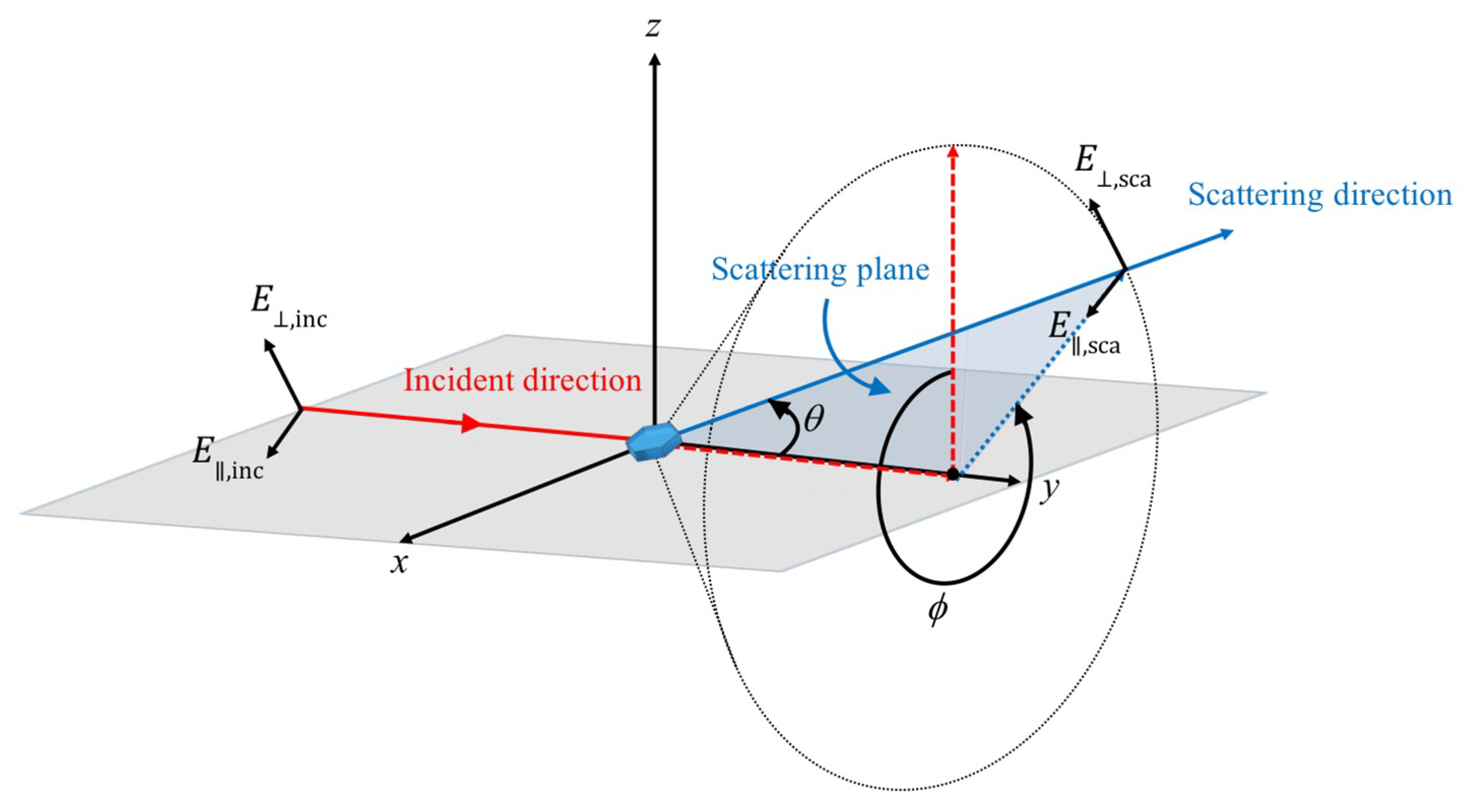
2. Theoretical Basis for the Optical Properties of Ice Clouds

Before we discuss the detailed optical properties of ice clouds, it is necessary to introduce several key optical and radiative properties involved in the transfer of radiation in a cloudy atmosphere. For atmospheric remote sensing applications based on the spectral or narrowband observations between 0.5 and 15 µm, the specification of a radiative quantity is essentially based on optical analysis (i.e., the relevant measurements are made by optical instruments). For this purpose, it is sufficient to use the Stokes vector to fully specify the radiation field, given the fact that two radiation beams with the same Stokes vector cannot be distinguished through optical analysis [54]. To define the Stokes vector, let us consider a plane electromagnetic wave. The electric vector of the wave can be decomposed into perpendicular and parallel components ($E_{//}$ and $E_{\perp }$) with respect to a given reference plane, as illustrated in Figure 1. In conjunction with the decomposition of the electric field vector, the Stokes vector, given by $I={(I,Q,U,V)}^T$ where the superscript T indicates matrix transpose, are defined as follows:

$$I=\frac{c}{8\pi }(E_{//}{E}_{//}^{*}+E_{\perp }{E}_{\perp }^{*}),$$

(1)

$$Q=\frac{c}{8\pi }(E_{//}{E}_{//}^{*}-E_{\perp }{E}_{\perp }^{*}),$$

(2)

$$U=\frac{c}{8\pi }(E_{//}{E}_{\perp }^{*}+E_{//}^{*}{E}_{\perp }),$$

(3)

$$V=i\frac{c}{8\pi }(E_{//}{E}_{\perp }^{*}-E_{//}^{*}{E}_{\perp }),$$

(4)

where the asterisk indicates the complex conjugation and $i=\sqrt{-1}$. The four elements of the Stokes vector are usually referred to as the Stokes parameters that have the dimension of irradiance. Among the Stokes parameters, I indicates the intensity of the radiation, Q and U indicate the state of linear polarization, and V indicates the state of circular polarization. An extensively used quantity is the degree of linear polarization (DLP) defined in the form [55,56]

$$DLP=\frac{\sqrt{Q^2+U^2}}{I}.$$

(5)

In the case of $U=0$, DLP is also defined in the form [57]

$$DLP=-\frac{Q}{I}.$$

(6)

Figure 2 shows the geometric configuration for the scattering of a plane electromagnetic wave propagating along the y-axis by a non-spherical particle. Both the incident and scattered electric vectors can be decomposed into parallel and perpendicular components with respect to the scattering plane, a plane containing the incident and scattering directions. The decomposition is described as follows:

$$\left(\begin{array}{c}{E}_{//}^s\\ E_{\perp }^s\end{array}\right)=\frac{\exp [ik(r-y)]}{-ikr}\left(\begin{array}{cc}{S}_2& S_3\\ S_4& S_1\end{array}\right)\left(\begin{array}{c}{E}_{//}^i\\ E_{\perp }^i\end{array}\right),$$

(7)

where the superscripts s and i indicate scattered and incident waves, respectively. k is referred to as the modified wavenumber, given by $k=2\pi /\lambda$ and $\lambda$ is the wavelength. r is the distance between the scattering particle and the observer in the radiation or far-field zone (r >>$\lambda$). $S_{i,\hspace{0.17em}i=1-4}$ are the elements of the amplitude scattering matrix. In the case of a non-spherical particle, without axial symmetry, the amplitude scattering matrix depends on not only the scattering zenith angle ($\theta$) but also the azimuthal angle ($\varphi$) of the scattering plane illustrated in Figure 2.

In conjunction with the transformation of the incident electric field to the scattered electric field in Equation (7), the corresponding transformation for the Stokes parameters is in the form

$$\left[\begin{array}{c}{I}^s\\ Q^s\\ U^s\\ V^s\end{array}\right]=\frac{F}{k^2{r}^2}\left[\begin{array}{c}{I}^i\\ Q^i\\ U^i\\ V^i\end{array}\right],$$

(8)

where matrix F is often referred to as the scattering Mueller matrix, which is a 4 × 4 matrix with elements that can be derived from the amplitude scattering matrix in Equation (7). For example, $F_{11}$ is given as follows:

$$F_{11}=(S_2\cdot S_2^{*}+S_3\cdot S_3^{*}+S_4\cdot S_4^{*}+S_1\cdot S_1^{*})/2,$$

(9)

The mathematical expressions for the other elements of matrix F are described in van de Hulst [58]. For many applications, e.g., in atmospheric remote sensing implementations and plane-parallel radiative transfer simulations, the scattering medium is assumed to be an ensemble of particles that are randomly oriented with equal numbers of mirror-imaging positions. The complexity greatly increases if the particles are given non-random orientations [59,60]. In this paper, we assume random orientations for the particles with equal numbers of mirror-imaging positions unless specifically defined otherwise. In this case, matrix F can be simplified in the following form [58,59,61]:

$$F=\left[\begin{array}{cccc}{F}_{11}& F_{12}& 0& 0\\ F_{12}& F_{22}& 0& 0\\ 0& 0& F_{33}& -F_{43}\\ 0& 0& F_{43}& F_{43}\end{array}\right].$$

(10)

Furthermore, matrix F in Equation (10) can be expressed in a normalized form as follows:

$$\begin{gathered} F=\left[\begin{array}{cccc}{F}_{11}& F_{12}& 0& 0\\ F_{12}& F_{22}& 0& 0\\ 0& 0& F_{33}& -F_{43}\\ 0& 0& F_{43}& F_{43}\end{array}\right] \\ =\frac{C_{sca}}{4\pi }P \\ =\frac{C_{sca}}{4\pi }\left[\begin{array}{cccc}{P}_{11}& P_{12}& 0& 0\\ P_{12}& P_{22}& 0& 0\\ 0& 0& P_{33}& -P_{43}\\ 0& 0& P_{43}& P_{43}\end{array}\right] \end{gathered}$$

(11)

where matrix P is generally referred to as the normalized scattering phase matrix, and $C_{sca}$ is the scattering cross section given by

$$C_{sca}=={\displaystyle {\int }_0^{2\pi }{\displaystyle {\int }_0^{\pi }{F}_{11}(\theta )\sin \theta d\theta d\phi }}.$$

(12)

In addition to the scattering cross section, one must also know the absorption cross section $C_{abs}$ to quantify the scattering particle’s capability of absorbing the incident radiation. The sum of the absorption and scattering cross sections provides the extinction cross section:

$$C_{ext}=C_{sca}+C_{abs}$$

(13)

For practical light-scattering computation, the extinction cross section is usually computed by using the amplitude scattering elements in the exact forward direction via the optical theorem [58]. The ratio of the scattering cross section to the extinction cross section is referred to as the single-scattering albedo, given by

$$\tilde{\omega }=C_{sca}/C_{ext}$$

(14)

The term $P_{11}(\theta )$ (usually called the phase function) is normalized by:

$$\frac{1}{4\pi }{\displaystyle {\int }_0^{2\pi }{\displaystyle {\int }_0^{\pi }{P}_{11}(\theta )\sin \theta d\theta d\phi }}=1$$

(15)

In many practical applications, we do not consider the detailed angular variation of the phase function. Instead, we introduce a parameter called the asymmetry factor $g$ to quantify the degree of the deviation of the scattered light from the incident direction, which is given by

$$g=<\cos \theta >=\frac{1}{4\pi }{\displaystyle {\int }_0^{2\pi }{\displaystyle {\int }_0^{\pi }{P}_{11}(\theta )\cos \theta \sin \theta d\theta d\phi }}$$

(16)

The above optical properties are referred to as the single-scattering properties for an individual particle. In practice, we need to consider an ensemble of scattering particles, which is referred to as a polydisperse system. The particle size distribution, $n(D)$ where D is the characteristic dimension specifying the size of the corresponding particle, has units of 1/volume/length (e.g., $1/c{m}^3/\mu m$). The physical meaning of the size distribution is that $n(D)dD$ is the number of particles per unit volume with particle characteristic dimensions between $D-dD/2$ and $D+dD/2$. For a given size distribution, the bulk extinction coefficient with units of per length is given by

$${\beta }_{ext}={\displaystyle {\int }_{D_{\min }}^{D_{\max }}{C}_{ext}(D)n(D)dD}.$$

(17)

To describe wavelength-dependent attenuation in a cloud given a dispersion of particles, a useful dimensionless quantity is the optical thickness, defined by

$$\tau ={\displaystyle {\int }_Z^{\infty }{\beta }_{ext}(z\prime )dz\prime }$$

(18)

where $z=\infty$ indicates the top of the atmosphere (TOA).

The above single-scattering properties are fundamental to the equation governing the transfer of radiation in a cloudy atmosphere. For example, in the case of plane-parallel atmosphere, the governing equation for radiance is given by

$$\begin{gathered} \mu \frac{dI(\tau ,\theta ,\phi )}{d\tau }=I(\tau ,\theta ,\phi )-\frac{\varpi }{4\pi }{\displaystyle {\int }_0^{2\pi }{\displaystyle {\int }_0^{\pi }I(\tau ,\theta ,\phi )P(\cos \mathsf{\Theta })\sin \theta d\theta d\phi }} \\ +(1-\varpi )B[T(\tau )] \end{gathered}$$

(19)

where I indicates the total (direct plus diffuse) radiance, B indicates Planck’s function associated with thermal emission, and $\cos \mathsf{\Theta }$ is the cosine of the scattering angle, given by

$$\mathsf{\Theta }={\cos }^{-1}[\sin \theta \sin \theta \prime \cos (\phi -\phi \prime )+\cos \theta \cos \theta \prime ].$$

(20)

Forward radiative transfer simulations based on Equation (19) are essential to the implementation of a remote sensing retrieval algorithm based on either LUTs or an inline radiative transfer solver. As the single-scattering properties are fundamental quantities in the radiative transfer equation, the use of the most representative bulk optical properties of cloud particles is crucial for simulating the radiation field accurately. Note that the choice of a representative bulk optical property model depends on the application. The model chosen for inference of global cloud properties based on a satellite imager may be quite different than the model chosen for a ground-based or aircraft-based sensor, or for a polarimeter where other elements of the phase matrix must be considered.

Early studies (e.g., [62]) assumed ice particles to be spherical, which is no longer a valid assumption given the numerous measurements of actual ice particles (e.g., [63,64,65,66,67]). Over the years, the research community has made significant progress towards solving for the optical properties of non-spherical particles from very small to very large size parameters, and from the UV through the far-infrared spectrum, from either theoretical or practical computational perspectives. Numerous light-scattering computational methods have been developed, including the separation of variables method for spheroids [68], the finite-difference time domain (FDTD) technique [69,70,71], the discrete dipole approximation (DDA) [72,73,74], the T-matrix method [75,76,77], and the geometric optical method and its improved counterparts [78,79,80,81,82,83,84,85]. Because light scattering by a non-spherical particle is a complicated subject, we do not review detailed light-scattering computational methods. An interested reader is referred to Mishchenko et al. [59,86] for non-spherical particles in general and Liou and Yang [4] for ice particles more specifically. In particular, we note that light scattering in the entire size parameter region may be effectively simulated by a synergetic combination of efficient implementations of the invariant imbedding T-matrix method [87] and the physical-optical method [83,84] in conjunction with recent improvements on its computational efficiency [88,89].

3. Ice Cloud Optical Models for Remote Sensing Applications

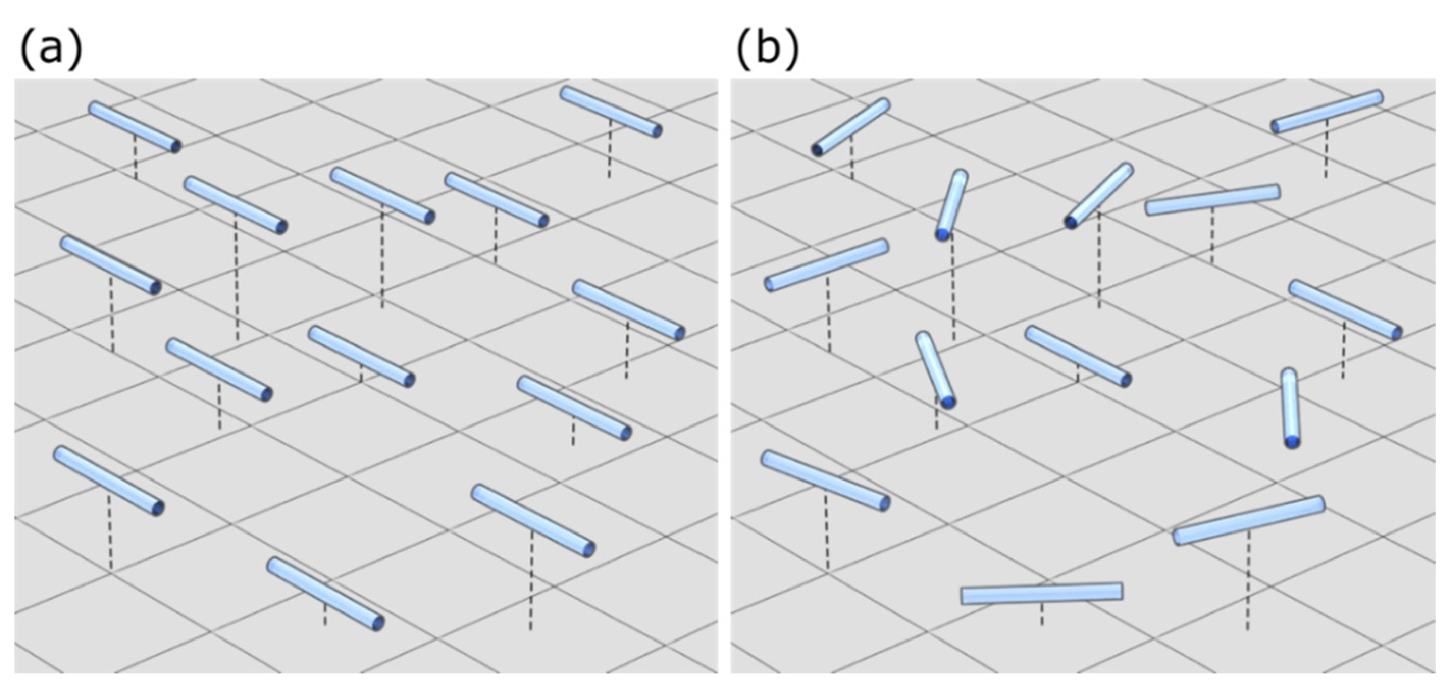
3.1. Ice Particle Shape and Orientation

Ice particles in the atmosphere are exclusively non-spherical particles (e.g., [63,64,90,91]). Beyond the spherical approximation for non-spherical ice particles, one of the earliest non-spherical models considered horizontally oriented cylinders [92], as illustrated in Figure 3. Specifically, ice particles are assumed to be long circular cylinders that are oriented horizontally in relation to their rotational axes. In Figure 3a, the cylinder axes point along the same direction, whereas, in Figure 3b, the cylinders are horizontally oriented in a random manner. While analytical light-scattering analysis for an infinitely long circular cylinder [93,94] is applied to approximate the single-scattering properties of a finite circular cylinder through an appropriate scaling procedure, Liou’s ice cloud models shown in Figure 3 were used by others (e.g., [95,96]) who showed that the significant differences in the single-scattering properties of spheres and cylinders resulted in pronounced difference in radiance simulations.

The scattering of light by oriented particles is quite complicated. As an example, Figure 4 shows the two-dimensional phase functions of an ensemble of hexagonal plates (Figure 4, upper panel) and hexagonal columns (Figure 4, lower panel) assuming a horizontally random orientation condition. The plates are randomly oriented in terms of their rotations around the asymmetry axes that are aligned vertically and columns are horizontally oriented with two parallel faces perpendicular to the vertical direction (known as Parry oriented columns). The physical-geometric optical computational program developed by Sun et al. [89] is used for this simulation.

As shown in Figure 4, the angular distribution of scattered energy associated with oriented ice particles is intriguing. For example, note that in the 2-D contour of the phase function of a horizontally oriented plate, there are two bright spots that correspond to a scattering polar angle of approximately 22°; these are the basic optical mechanism of sundogs shown in Figure 5a [4,97].

The false color image in Figure 5a is produced by combining the radiance simulations at three wavelengths in a false color composite (Red:Green:Blue (RGB) form of Red: $I_{1.064\mu m}\times 3$, Green: $I_{0.532\mu m}\times 0.7$, and Blue: $I_{0.355\mu m}\times 2$). Only 7.9% of plates are assumed to be horizontally oriented, whereas 92.1% of the particles are 3-D randomly oriented. The simulated radiances are mapped to the coordinates of fish-eye camera image. In Figure 5a, note the presence of an optical phenomenon called a sun pillar in addition to the sundogs [98]. The 2-D phase function of the Parry oriented columns shown in Figure 4 has complexities that may be captured with appropriate sensor measurements under single scattering conditions. The false color image in Figure 5b is produced by combining the radiance simulations at three wavelengths (Red: 610 nm, Green: 532 nm, and Blue: 460 nm) by assuming an optically thin ice cloud consisting of 100% Parry ice columns. Multiple scattering effects are excluded in the simulations. Note that rare optical phenomena such as helic, subhelic, and Parry infralateral arcs ([4], and the references cited therein) are reproduced in Figure 5b.

The preceding discussion leads to a question: Is it a valid simplification to assume that ice particles are randomly oriented in the atmosphere for passive remote sensing applications? Fortunately, measurements made by CALIOP aboard CALIPSO provide unprecedented observations to quantify atmospheric ice particle orientations. In particular, Hu et al. [99] showed that the relationship between the layer-averaged attenuated backscatter (γ) and layer-averaged depolarization ratio (δ) from the CALIPSO measurements can be used to effectively discriminate between horizontally oriented and 3-D randomly oriented ice particles. Here, γ and δ are defined as [99]

$$\delta =\frac{{\displaystyle {\int }_{\mathrm{cloud} \mathrm{top}}^{\mathrm{cloud} \mathrm{base}}{\beta }_{b,\perp }(z)dz}}{{\displaystyle {\int }_{\mathrm{cloud} \mathrm{top}}^{\mathrm{cloud} \mathrm{base}}{\beta }_{b,//}(z)dz}},$$

(21)

$$\gamma ={\displaystyle {\int }_{\mathrm{cloud} \mathrm{top}}^{\mathrm{cloud} \mathrm{base}}[{\beta }_{b,//}(z)+{\beta }_{b,\perp }(z)]dz},$$

(22)

where ${\beta }_{b,\perp }$ and ${\beta }_{b,//}$ are the perpendicular and parallel components of the attenuated backscatter observed at CALIOP 0.532-µm channel, respectively. Hu et al. [99] explained that, in the γ-δ relation shown schematically in Figure 6a, the segment corresponding to strong backscatter and low depolarization ratio is associated with horizontally oriented ice particles, whereas the segment corresponding to weak backscatter and large depolarization ratio is associated with 3-D randomly oriented ice particles. In following Hu et al. [99] to investigate the aforementioned theoretical speculation, Figure 6b shows the CALIOP data for the γ-δ relation as observed during April 2007. At that time, the CALIOP lidar was in a nadir-viewing configuration and the specular reflection by horizontally oriented ice particles was so substantial that the lidar pointing configuration was soon adjusted to point away from nadir. Figure 6c is similar to Figure 6b except the data were obtained during April 2009 when CALIOP lidar pointed 3º off the nadir. In the case of Figure 6c, the specular reflection is not observed by the lidar receiver and the segment of large γ and small δ is missing in Figure 6c. The comparison of panels 6b and c of Figure 6 unequivocally confirms the existence of oriented ice particles.

With observations made by CALIOP and the Infrared Imaging Radiometer (IIR), both of which are on the CALIPSO platform, Saito et al. [100] derived the percentage of oriented ice particles. The results are shown in Figure 7. The fraction of oriented ice particles is less than 1% at cloud temperatures warmer than −30 °C but further decreases with temperature. These results are essentially consistent with those by Zhou et al. [101] and Chepfer et al. [102]. Based on the current evidence, it is quite reasonable to assume ice particles to be randomly oriented for passive remote sensing applications that do not involve polarimetric measurements. Note that polarimetric microwave measurements are sensitive to hydrometeor orientations [26], and the assumption may introduce errors in ice cloud retrievals based on the measurements. With the assumption of the random orientation condition for the scattering particles, the single-scattering properties and the equation of radiative transfer are significantly simplified. Specifically, the phase matrix depends only on the scattering polar angle and is independent of the azimuthal angle of the scattering plane. The phase matrix is in a diagonal-block form as in Equation (10) (note: the diagonal-block form implies that the particles have an equal number of mirror-imaging orientations in addition to the random orientation condition). Furthermore, a scalar extinction coefficient can be used instead of the extinction matrix for radiative transfer simulations.

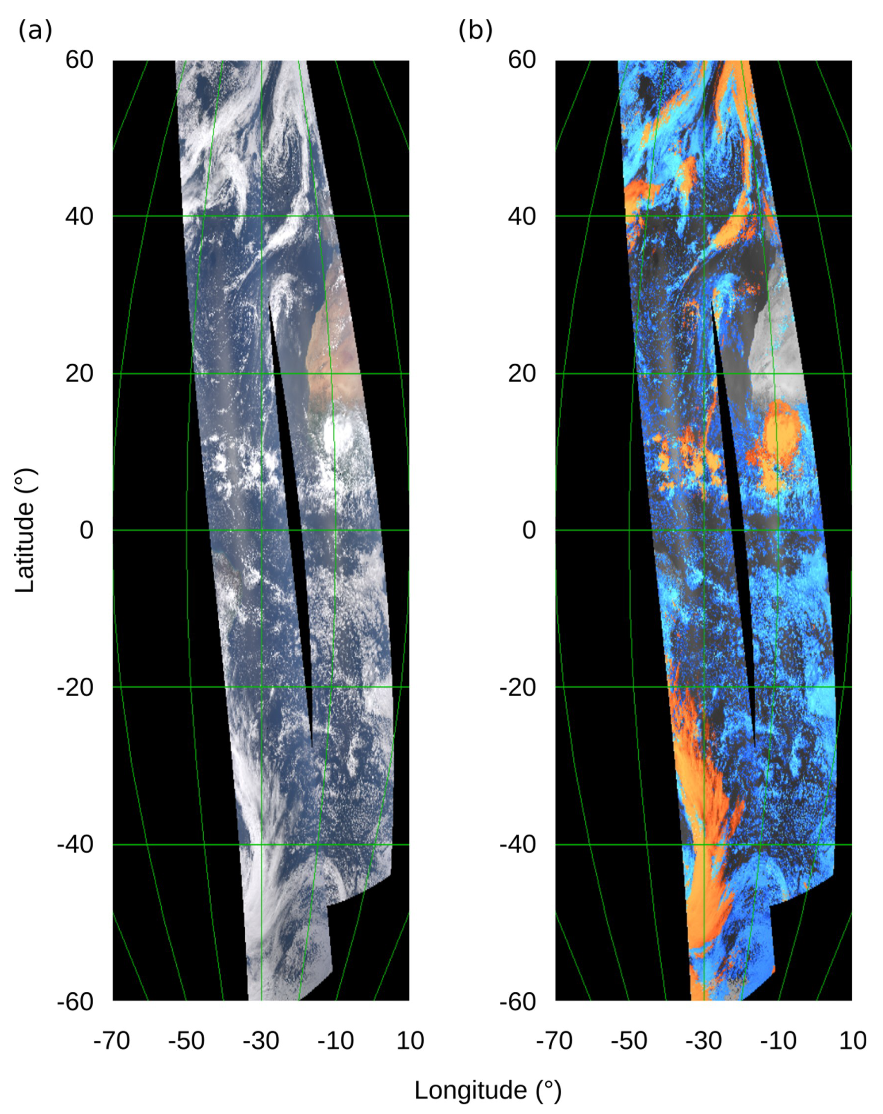
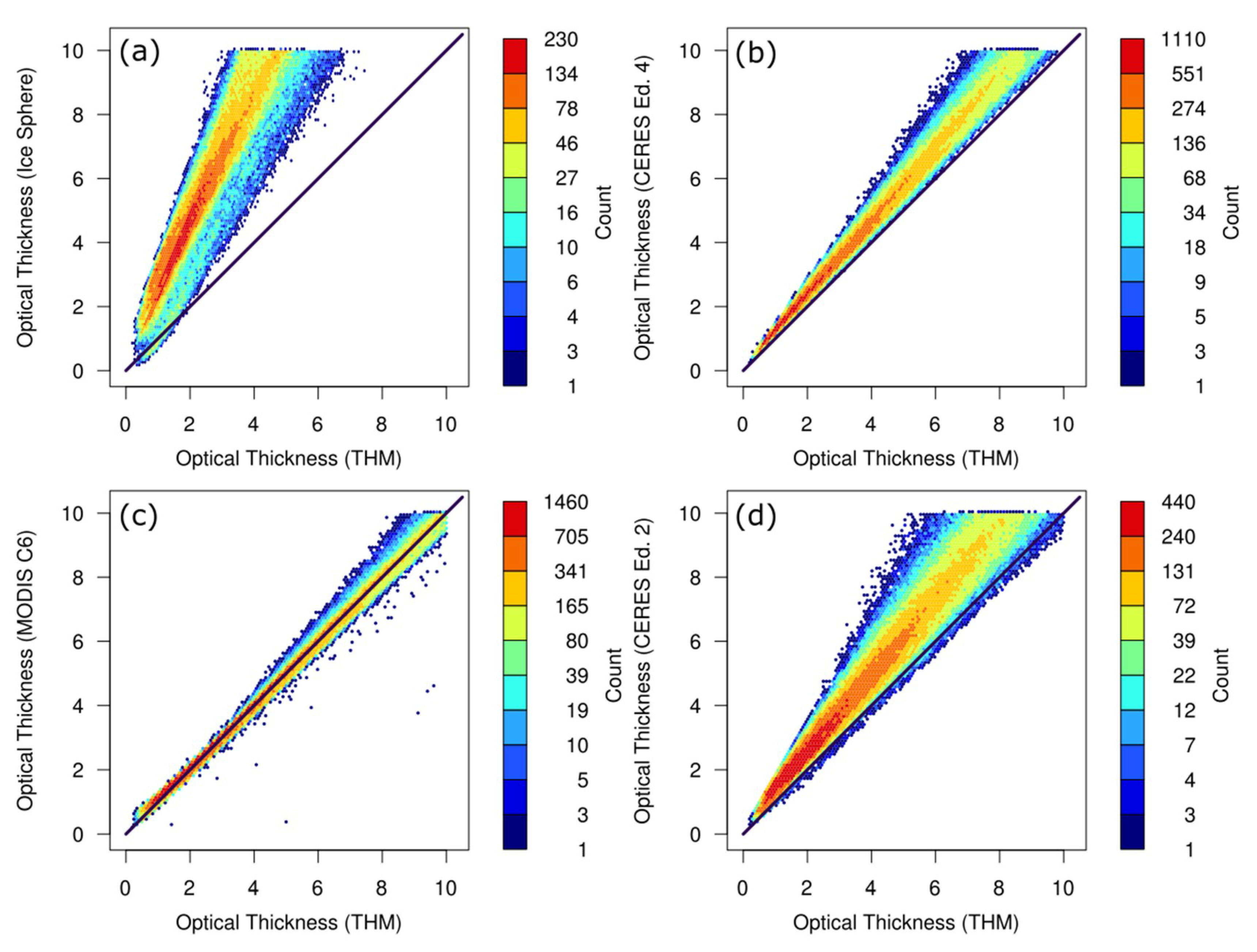
3.2. Bulk Optical Properties for Passive Remote Sensing Applications

For passive remote sensing applications, the first group of ice particle models discussed here includes three models developed by the MODIS science team. The MODIS science team applies the Nakajima–King bi-spectral method [42] to simultaneously retrieve cloud optical thickness and effective particle size. As illustrated in Figure 8, the reflectivity correlation between a pair of MODIS channels contain information about cloud optical thickness and effective particle size. The information content stems from the fact that, in a conservative scattering channel (e.g., a channel centered at 0.85 µm), ice cloud reflectivity is insensitive to the effective particle size while the reflectivity at weakly absorbing shortwave-infrared channel (e.g., a channel centered at 2.13 µm) depends on both optical thickness and effective particle size. In particular, the optical thickness isolines are orthogonal to the effective particle size isolines at large optical thicknesses, allowing straightforward retrievals of the two parameters given a sufficiently high optical thickness. In the literature, there are several forms to define ice cloud effective particle size, but the following definition gives consistent definitions in both the cases of water and ice clouds [103,104]:

$$r_{eff}=\frac{3}{4}\frac{V_{total}}{A_{proj,total}},$$

(23)

where $V_{total}$ and $A_{proj,total}$ are the total volume and projected area, respectively, given by

$$V_{total}={\displaystyle {\int }_{r_{\min }}^{r_{\max }}V(r)n(r)dr},$$

(24)

$$A_{proj,total}={\displaystyle {\int }_{r_{\min }}^{r_{\max }}{A}_{proj}(r)n(r)dr}.$$

(25)

In Equations (24) and (25), r indicates half of the maximum characteristic dimension (i.e., the radius in the case of a sphere) of an individual particle. In the case of a water cloud consisting of spherical droplets, Equation (23) reduces to

$$\begin{gathered} r_{eff}=\frac{3}{4}\frac{{\displaystyle {\int }_{r_{\min }}^{r_{\max }}(4\pi r^3/3)n(r)dr}}{{\displaystyle {\int }_{r_{\min }}^{r_{\max }}(\pi r^2)n(r)dr}}, \\ =\frac{{\displaystyle {\int }_{r_{\min }}^{r_{\max }}{r}^{3}n(r)dr}}{{\displaystyle {\int }_{r_{\min }}^{r_{\max }}{r}^{2}n(r)dr}} \end{gathered}$$

(26)

The definition given in Equation (26) is exactly the same as that in Hansen and Travis [103] for water cloud particles assumed to be spherical. Thus, Equation (23) is a rational extension of the definition introduced by Hansen and Travis to non-spherical ice cloud particles. Another advantage of the definition by Equation (23) is that the ice water path (IWP) can be expressed in the form

$$\begin{gathered} IWP=\frac{4}{3}\frac{{\rho }_{ice}}{<Q_{ext}>}{r}_{eff}\tau , \\ \approx \frac{2}{3}{\rho }_{ice}{r}_{eff}\tau , \end{gathered}$$

(27)

where ${\rho }_{ice}=0.916g/c{m}^3$ is the mass density of bulk ice, and <Q_ext> is the mean extinction efficiency given by

$$<Q_{ext}>=\frac{{\displaystyle {\int }_{r_{\min }}^{r_{\max }}{Q}_{ext}(r)A_{proj}(r)n(r)dr}}{{\displaystyle {\int }_{r_{\min }}^{r_{\max }}{A}_{proj}(r)n(r)dr}}\approx 2.$$

(28)

A complementary approach for inferring the optical properties when the optical thickness is lower than the optimal range for a reflectance-based method in the VIS-SWIR bands is to use split-window measurements in infrared channels at 11 µm and 12 µm (e.g., [105]). These measurements are provided by most weather satellite imagers. Figure 9 shows the look-up table constructed by split-window measurements from MODIS bands 31 and 32 (11 µm and 12 µm, respectively).

To estimate an optimal solution of a state vector (x) in the look-up table generated by the Nakajima–King bi-spectral method or split-window IR measurements, we use a maximum likelihood method [106] by minimizing a cost function (J) given by

$$J={\left[y-F\left(x\right)\right]}^T{S}_y^{-1}\left[y-F\left(x\right)\right],$$

(29)

where y, F(x), and S_y are the measurement vector, the forward model, and the measurement error covariance matrix, respectively. The errors of the retrieved state and measurement vectors are assumed to follow normal distributions. Furthermore, we assume that there is no correlation between measurement errors. The forward model employs the correlated-K method [107] to account for gas absorption and the discrete ordinate radiative transfer (DISORT) model [108] or the adding-doubling method [109,110] for radiance simulations.

The retrieval process is schematically shown in Figure 9. Based on an initial state vector, x = (τ₁, D_e1)^T, we obtain an updated state vector, x = (τ₂, D_e2)^T from a Jacobian matrix in conjunction with the Newton method. Then, we proceed this process iteratively to finally obtain the optimal state vector, x = (τ₃, D_e3)^T, which meets a criterion of the cost function (J ~ m, where m is the number of elements of the measurement vector) [106]. In this study, retrievals of ice clouds are conducted over ocean, and the atmospheric profiles and ocean surface temperature are provided by ECMWF reanalysis data.

In the computation of MODIS particle models (see Figure 10), the definition of maximum dimension ($D_{max}$) depends on particle habits. $D_{max}$ is defined as the particle height for a hexagonal (solid and hollow) column, diameter of basal facets for a hexagonal plate, and the longest distance between two vertices for a column aggregate, bullet rosette, or droxtal. The mixed scattering properties averaged over the particle size distribution are called “bulk” scattering properties. The precise definitions of the bulk properties were summarized by Baum et al. [111]. The other important information necessary for the derivation of the bulk scattering properties is knowledge of the particle size distribution (PSD). Historically, the PSDs have been defined for this effort in two ways for ice cloud remote sensing by passive imagers: using a well-defined gamma distribution or in-situ measurements. The obvious benefit of using a gamma distribution is that one has total control over the size limits and width of the PSD. The use of actual in-situ data is much more involved than the use of analytical PSDs, but the relevant bulk single-scattering models can be assessed for different dynamical regimes (e.g., low updraft velocity such as synoptic cirrus versus tropical anvils formed in a convective dynamical environment). Different approaches may be adopted for active sensors, which can sense much larger particles and infer much higher values of IWP, and millimeter to sub-millimeter measurements [27].

Among the aforementioned three ice particle models employed for the calculation of ice cloud bulk scattering properties, the first model (Figure 10a) was employed in MODIS Collection 4 [112,113]. The particle habit fractions are fixed in either a small or large particle regime as follows: (1) 50% four-element bullet rosettes, 25% hexagonal plates, and 25% hollow columns for $D_{max}<70$ µm; and (2) 30% aggregates, 30% bullet rosettes, 20% hexagonal plates, and 20% hollow columns for $D_{max}>70$ µm. The bulk properties are calculated by integrating the single scattering properties over only twelve PSDs, each of which is discretized in terms of five coarse size bins (10–30, 3–70, 7–170, 170–430, and 430–1070 µm). For the 12 PSDs, the effective particle radii are 6.7, 9.6, 14.5, 19.7, 25.0, 28.0, 32.0, 40.0, 47.4, 48.6, 50.7, and 58.9 µm. The effect of the particle-size bin resolution was studied by Nasiri et al. [114], who basically found that a finer discretization was necessary. Liu et al. [115] found that a high bin resolution in terms of using the kernel technique can uncover more nuanced information of the bulk microphysical and optical properties of ice particles.

Given the coarseness of the MODIS Collection 4 model, effort was made to increase the library of ice particle single scattering properties (e.g., [116,117]). Based on improvements in both the library of single scattering properties and the use of microphysical PSD data archived from various field campaigns, a second model [118,119], illustrated in Figure 10b, was developed for MODIS Collection 5. The model was more complex because single scattering properties were available in 45 size bins, with habit fractions as follows: (1) 100% droxtals for $D_{max}<60$ µm; (2) 50% solid columns, 35% hexagonal plates, and 15% six-element bullet rosettes for $60<D_{max}<1000$ µm; (3) 45% solid columns, 45% hollow columns, and 10% column aggregates for $1000<D_{max}<2000$ µm; and (4) 97% bullet rosettes and 3% column aggregates for $D_{max}>2000$ µm [118]. These particle habit mixtures were determined to best explain 1117 samples of airborne in-situ particle size distributions, ice water contents, median mass diameters, and pictures of ice particles captured during the field campaigns. While bulk single-scattering properties were computed for each of the 1117 particle size distributions, the single-scattering properties used in retrievals were based on an average of 10–20 size distributions distributed around each of 18 target effective diameters [119]. The MODIS Collection 5 ice model was also used for AIRS version 6 retrievals [35].

While the MODIS Collection 5 models were based on a set of 1117 different PSDs, the measurements detailed in [90] greatly increased the number of available PSDs by an order of magnitude, with resulting ice cloud bulk single-scattering models detailed in [120] for visible through far-infrared wavelengths.

The most current model used by the MODIS science team is that for the operational MODIS Collection 6 [18]. As shown in Figure 10c, the MODIS Collection 6 model is rather straightforward in terms of particle habit: it consists solely of aggregates of severely roughened hexagonal column particles, regardless of particle maximum dimension, and gamma particle size distributions are assumed with a fixed effective variance parameter ($v_{eff}=0.1$). The development of the MODIS collection 6 ice cloud model was largely motivated by the consistency between shortwave-based and IR-based retrievals [18,121].

In addition to the MODIS science team, the CERES science team retrieves cloud properties as part of its data reduction effort. Both the MODIS and CERES sensors are on the EOS-Aqua and EOS-Terra platforms. CERES has employed two different ice particle models to date, with a new two-habit model in development. CERES Edition 2 and Edition 3 products used smooth hexagonal column particle models based on eight discrete size bins and ten particle size distributions from measurements by airborne field campaigns [122,123,124,125]. Edition 4 keeps the particle shape and particle size distributions the same, while applying surface roughness to the particle model. The planned Edition 5 may use a two-habit model [126]. Figure 11 schematically depicts the CERES Edition 2 through five particle models. The two-habit model consists of a roughened hexagonal column and the ensemble average of 20 random aggregates of 20 distorted hexagonal columns. The proportion of the single column is defined as follows to satisfy the in-situ airborne measurements:

$$f_{column}=\{\begin{array}{c}1, D_{\max }\le 30 \mu m\hspace{1em}\\ \exp [-0.005(D_{\max }-30), D_{\max }\le 30 \mu m,\end{array}$$

(30)

and the proportion of the aggregate column is obtained by $f_{aggregate}=1-f_{column}$.

In MODIS Collection 4 and 5 models, the ice particles are assumed to have smooth surfaces, with the exception of the aggregate particle that is assumed to be moderately roughened. Because smooth particles dominate in these ice models, the corresponding phase functions have angularly dependent features that are evident in the phase function comparison between MODIS Collections 5 and 6 in Figure 12. The phase function of the MODIS Collection 6 is featureless because particle surface roughness smooths out the scattering peaks and maxima. Additionally, the asymmetry parameter increases with particle size for solar wavelengths in both the Collection 4 and 5 bulk models, while the asymmetry parameter is essentially independent of particle size for the Collection 6 model (Figure 13).

For two clouds with optical properties (specifically, optical thickness and the asymmetry factor) in a non-absorbing band $(\tau ,g)$ and $(\tau \prime ,g\prime )$, a quasi-invariant relation known as the similarity relation [127,128] holds:

$$\tau (1-g)\approx \tau \prime (1-g\prime ).$$

(31)

With the CERES Edition 2 model and the two-habit model as an example for comparison, it is straightforward to speculate that the optical thickness values retrieved with the two-habit model are smaller than their counterparts based on the CERES Edition 2 model. This is because ${\tau }_{THM}\approx {\tau }_{Edition2}(1-g_{Edition2})/(1-g_{THM})$ from Equation (31) and $(1-g_{Edition2})/(1-g_{THM})<1$, as evident in the upper middle panel of Figure 13.

Recent studies based on measurements from sensors in the NASA A-Train [129] indicate that, to obtain ice cloud properties that are more independent of the sensor, it is important to include a mechanism that acts to randomize the scattering within an ice particle, so that the phase function has reduced halo features. This finding has been the result of various sensor comparisons. Comparisons between results using the MODIS ice models and CALIOP measurements have shown that a roughened particle is preferred (e.g., [111,121]). Comparisons between MODIS Collection 5 and POLDER indicate that certain ice habits better match the polarization measurements and also indicate particles should not have smooth facets [120,130,131]. Given the variety and scope of current sensors, our goal is to work towards construction of an ice model that minimizes differences in ice cloud properties based on observations made by various sensors.

3.3. Spectral Consistency of Bulk Ice Particle Models

Polarization measurements by the POLDER sensor illustrate an aspect of the intrinsic consistency of ice cloud models for solar channels. The modified polarized reflectance product (or equivalently, modified polarized normalized reflectance) is not sensitive to cloud optical thickness when clouds are optically thick (τ > 4) but is sensitive to the selection of ice cloud models. In this study, we analyzed the modified polarized reflectance product in comparison with model simulations based on the CERES Edition 2 model and the two-habit model. Here, the modified polarized reflectance product is defined as [132]

$$L_{nmp}\left(\mu ,{\mu }_0,\phi ,{\phi }_0\right)=\eta \frac{\pi \sqrt{Q^2+U^2}}{E_0{\mu }_0}\left({\mu }_0+\mu \right),$$

(32)

where $E_0{\mu }_0$ is the flux density crossing through a horizontal plane, $E_0$ is the beam irradiance, and η is the sign (±1) defined by C.-Labonnote et al. [132].

Figure 14 shows the distribution of cloud pixels of POLDER observations that are used for the following analyses shown in Figure 15. We selected pixels in September 2006 that meet the following criteria: (1) ice phase clouds; (2) MODIS Band 31 (11 µm) brightness temperatures < 233 K; (3) the cloud optical thickness > 4; and (4) POLDER measurements over ocean. We sampled these pixels on a global scale to test the two-habit model because the model is intended to be used globally for retrieval of ice cloud properties. The first two criteria ensure that ice particles are present at cloud top. Optically thin cirrus clouds and ice cloud over land were removed from the analysis to reduce uncertainty associated with surface reflectance. Many cloud pixels are located in the midlatitude storm tracks and in the tropics, especially over Maritime continent and tropical Indian Ocean. Because there is more land cover in the northern hemisphere, the Southern Ocean contributes significantly to the midlatitude data collection. As September is in the tropical cyclone season for the northern hemisphere, the temporal sampling window is primarily responsible for the contrast of the data population in the northern and southern subtropics. In total, 283,594 pixels met our criteria and were used for the analysis.

Figure 15 shows the probability density distribution of the modified polarized reflectance from the POLDER observations and the counterparts from the simulations assuming the two-habit model and the CERES Edition 2 model. Overall, the observed modified polarized reflectance decreases with increasing the scattering angle over a range of 100–170°. The simulations based on the two-habit model closely match with those from the observations except at the scattering angles with 100–120° because of the weak polarized side scattering by the Two-habit model, whereas the simulations based on the CERES Edition 2 substantially deviate from the observations. Therefore, the two-habit model is much more appropriate than the CERES Edition 2 model in terms of the consistency between the model-based modified polarized reflectance and the measured counterparts at the scattering angles within 100–170°.

Furthermore, to demonstrate the dependence of retrieved cloud properties on particle habit, we present results from shortwave (SW) and longwave (LW) retrievals. The data were acquired by Aqua MODIS over the ocean at latitudes between 55°S and 50°N for two orbits on 10 September 2006. The visible composite image and the MODIS cloud phase are presented in Figure 16. The analysis was limited to pixels that are identified as ice by the MODIS Collection 6 cloud flag and with optical thickness less than 4. The results indicate that SW and LW retrievals are consistent with use of the two-habit or MODIS Collection 6 ice particle model.

Figure 17 shows the comparison of the retrieved optical thickness from SW and LW techniques. In the upper left panel of Figure 17, it can be seen that, if ice particles are assumed to be spheres, the optical thicknesses retrieved with the IR split window technique are much smaller than their counterparts based on the solar bands using the Nakajima–King algorithm. Thus, spectral consistency in the retrieval is not achieved for the spherical model. This is also true for the CERES Edition 2 model (upper right panel of Figure 17). However, it can be seen in the two lower panels of Figure 17 that both the MODIS C6 model and THM lead to spectrally consistent retrievals for optical thickness up to 3. For larger optical thicknesses, the IR signals at TOA lose sensitivity to the lower portion of the cloud and thus the IR band retrievals are systematically lower than the solar band counterparts. The solar and IR based methods are complementary in this respect, with the IR-based method having greater sensitivity to lower optical thicknesses than the solar method. Based on the comparisons shown in Figure 17, it can be said that both the MODIS C6 model and THM are optimal from the perspective of spectral consistency in retrieving ice cloud properties.

Figure 18 and Figure 19 show the optical thickness retrieved using different ice particle models by the VIS-SWIR bi-spectral technique. The retrievals were performed from Terra MODIS data acquired over ocean between 55° S and 50° N over a week from 12 to 18 September 2013. Figure 18 indicates that optical thickness values are consistent when retrieved with the MODIS Collection 6 model and two-habit model. The scatter plots for a spherical ice particle model (Figure 18a) and CERES Edition 2 (Figure 18d) have significantly broader distributions than (Figure 18b) CERES Edition 4 and (Figure 18c) MODIS Collection 6 models.

Figure 19 shows the ratios of optical thicknesses between four different ice models and the two-habit model to show consistency/inconsistency between models. In this figure, there are approximately 30,000 data points for every 10° scattering angle bins centered at about 90° to 170°. As indicated in these results, the best consistency is shown between the CERES Edition 4 model to two-habit model in Figure 19b, and between the MODIS Collection 6 model to two-habit model in Figure 19c. The comparisons involving the CERES Edition 2 model and the ice spheres show the least consistency. If the goal is to be able to compare products from different teams, this sort of information is critical for understanding the strengths and weaknesses of the products, and for modelers to make sense of them.

In addition to the ice cloud models discussed above, an inhomogeneous ice particle model (Figure 20a) was developed for ice cloud property retrieval from POLDER observations [132] and an ice cloud model based on the Voronoi shape (Figure 20b) was developed for retrievals from the Himawari-8 AHI observations [133,134]. Moreover, van Diedenhoven et al. [135,136] assumed hexagonal particles with incorporation of surface roughness for retrievals based on airborne scanning polarimetric measurements. A thorough comparison is made between the POLDER and MODIS Collection 5 ice cloud optical property models in [137]. A case study in [137] shows ${\tau }_{POLDER}\approx 0.7{\tau }_{MODIS}$, illustrating the sensitivity of the retrieved ice cloud optical thickness to the forward optical property model used in implementing the retrieval algorithm.

4. Summary

In this review, we survey recent studies related to the construction of ice cloud bulk scattering models and some of the choices that teams made for their derivation. We review the history of the development of ice cloud models, beginning with an early model assuming ice particles to be horizontally oriented circular cylinders, and moving to the models being used in current satellite retrieval products. We discuss whether horizontally-oriented particles exist in ice clouds, and to what degree. This analysis is based on CALIOP data analysis. This is important because ice particle orientation increases the complexity of ice particle single-scattering properties. We illustrate that it is valid to assume that ice particles are randomly oriented in the atmosphere for passive remote sensing purposes without considering particle orientation.

While a team may construct these ice models for a single sensor, there is increasing work being done to enhance the consistency of cloud property retrievals across a variety of spaceborne sensors. That is, there is more work being done to merge data from multiple sensors to improve the ice cloud retrievals, and subsequently to compare the satellite-based ice cloud properties with those from models. One would hope that the ice cloud properties derived from two sensors on the same platform, e.g., VIIRS (an imager) and CrIS (a hyperspectral IR sounder) would result in consistent global products. As noted in this review, there is a tendency for each team to develop their own ice cloud bulk single-scattering model in isolation. For example, there are teams that use a gamma particle size distribution and a single ice habit, and other teams that make more extended use of in-situ microphysical measurements of PSDs and different habits. Since various retrieval teams may develop an ice bulk scattering model that fits their needs, there must be studies that compare the results between sensor teams. Our goal is to reach better consistency in retrievals from imagers, hyperspectral infrared sounders, polarimeters, and active lidar measurements. This will extend in the future to encompass millimeter and sub-millimeter measurements and perhaps polarimetric measurements over a broader spectral range.

As examples shown in this study, comparisons of optical thickness are made between a visible-shortwave infrared technique and an infrared channel technique. We demonstrate that the MODIS Collection 6 model and the CERES two-habit model give spectrally consistent retrievals of ice cloud microphysical and optical properties. Additionally, the same bulk scattering models are used to compare results from a space-based polarimeter (POLDER). These two models incorporate severely roughened particle surfaces that lead to featureless bulk phase functions. At present, the MODIS Collection 6 and the CERES two-habit models are optimal ice particle models for passive remote sensing of global ice clouds. Polarimetric-based observations of ice clouds tend to focus on ice particles near the top of the cloud, while shortwave-infrared channels may penetrate the ice cloud to different depths. Infrared-based ice cloud retrievals have a more limited optical thickness range due to the increased particle absorption. Active sensors provide a wealth of information about the columnar ice cloud optical/radiative and microphysical properties but the measurements are limited by their narrow beams. With the effort to assemble multiple datasets, there is then an opportunity to gain a wider perspective of the range of ice cloud optical/radiative and microphysical properties. The eventual goal is to find a framework for inferring these properties, which leads to more consistent results across the sensors where new measurements can add to the body of knowledge of ice clouds.

References

1. Liou, K.N. Influence of cirrus clouds on weather and climate processes—A global perspective. Mon. Weather Rev. 1986, 114, 1167–1199. [Google Scholar] [CrossRef]
2. Baran, A.J. A review of the light scattering properties of cirrus. J. Quant. Spectrosc. Radiat. Transf. 2009, 110, 1239–1260. [Google Scholar] [CrossRef]
3. Baran, A.J. From the single-scattering properties of ice crystals to climate prediction: A way forward. Atmos. Res. 2012, 112, 45–69. [Google Scholar] [CrossRef]
4. Liou, K.N.; Yang, P. Light Scattering by Ice Crystals: Fundamentals and Applications, 1st ed.; Cambridge University Press: Cambridge, UK, 2017. [Google Scholar]
5. Zhang, M.; Lin, W.Y.; Klein, S.A.; Bacmeister, J.T.; Bony, S.; Cederwall, R.T.; Del Genio, A.D.; Hack, J.J.; Loeb, N.G.; Lohmann, U.; et al. Comparing clouds and their seasonal variations in 10 atmospheric general circulation models with satellite measurements. J. Geophys. Res. 2005, 110, D15S02. [Google Scholar] [CrossRef]
6. Ahrens, C.D.; Henson, R. Meteorology Today: An Introduction to Weather, 12nd ed.; Cengage Learning: Boston, MA, USA, 2018. [Google Scholar]
7. Liou, K.N. Radiation and Cloud Processes in the Atmosphere: Theory, Observation, and Modeling; Description and Reviews; Oxford University Press: New York, NY, USA, 1992; 487p. [Google Scholar]
8. Wylie, D.P.; Menzel, W.P. Eight years of high cloud statistics using HIRS. J. Clim. 1999, 12, 170–184. [Google Scholar] [CrossRef]
9. Rossow, W.B.; Schiffer, R.A. ISCCP cloud data products. Bull. Am. Meteorol. Soc. 1991, 72, 2–20. [Google Scholar] [CrossRef]
10. Stubenrauch, C.J.; Rossow, W.B.; Kinne, S.; Ackerman, S.; Cesana, G.; Chepfer, H.; Di Girolamo, L.; Getzewich, B.; Guignard, A.; Heidinger, A.; et al. Assessment of global cloud datasets from satellites: Project and database initiated by the GEWEX radiation panel. Bull. Am. Meteorol. Soc. 2013, 94, 1031–1049. [Google Scholar] [CrossRef]
11. Massie, S.; Gettleman, A.; Randel, W.; Baumgardner, D. The distribution of tropical cirrus in relation to convection. J. Geophys. Res. 2002, 107. [Google Scholar] [CrossRef]
12. Waliser, D.E.; Li, J.-L.F.; Woods, C.P.; Austin, R.T.; Bacmeister, J.; Chern, J.; Del Genio, A.; Jiang, J.H.; Kuang, Z.; Meng, H.; et al. Cloud ice: A climate model challenge with signs and expectations of progress. J. Geophys. Res. 2009, 114. [Google Scholar] [CrossRef]
13. Elsaesser, G.S.; Del Genio, A.D.; Jiang, J.; van Lier-Walqui, M. An improved convective ice parameterization for the NASA GISS Global Climate Model and impacts on cloud ice simulation. J. Clim. 2016, 30, 317–336. [Google Scholar] [CrossRef]
14. Deng, M.; Mace, G.G.; Wang, Z.; Lawson, R.P. Evaluation of Several A-Train Ice Cloud Retrieval Products with In Situ Measurements Collected during the SPARTICUS Campaign. J. Appl. Meteorol. Climatol. 2013, 52, 1014–1030. [Google Scholar] [CrossRef]
15. Deng, M.; Mace, G.G.; Wang, Z.; Berry, E. CloudSat 2C-IE product update with a new Ze parameterization in lidar-only region. J. Geophys. Res. Atmos. 2015, 120, 12198–12208. [Google Scholar] [CrossRef] [PubMed]
16. Heidinger, A.K.; Foster, M.J.; Walther, A.; Zhao, X. The pathfinder atmospheres-extended AVHRR climate dataset. Bull. Amer. Meteorol. Soc. 2014, 95, 909–922. [Google Scholar] [CrossRef]
17. King, M.D.; Menzel, W.P.; Kaufman, Y.J.; Tanre, D.; Gao, B.C.; Platnick, S.; Ackerman, S.A.; Remer, L.A.; Pincus, R.; Hubanks, P.A. Cloud and aerosol properties, precipitable water, and profiles of temperature and water vapor from MODIS. IEEE Trans. Geosci. Remote Sens. 2003, 41, 442–458. [Google Scholar] [CrossRef] [Green Version]
18. Platnick, S.; King, M.D.; Ackerman, S.A.; Menzel, W.P.; Baum, B.A.; Riedi, J.C.; Frey, R.A. The MODIS cloud products: Algorithms and examples from Terra. IEEE Trans. Geosci. Remote Sens. 2003, 41, 459–473. [Google Scholar] [CrossRef]
19. Lee, T.E.; Miller, S.D.; Turk, F.J.; Schueler, C.; Julian, R.; Deyo, S.; Dills, P.; Wang, S. The NPOESS VIIRS day/night visible sensor. Bull. Am. Meteorol. Soc. 2006, 87, 191–199. [Google Scholar] [CrossRef]
20. Skofronick-Jackson, G.; Petersen, W.A.; Berg, W.; Kidd, C.; Stocker, E.F.; Kirschbaum, D.B.; Kakar, R.; Braun, S.A.; Huffman, G.J.; Iguchi, T.; et al. The Global Precipitation Measurement (GPM) Mission for Science and Society. Bull. Am. Meteorol. Soc. 2017, 98, 1657–1672. [Google Scholar] [CrossRef]
21. Hou, A.Y.; Kakar, R.K.; Neeck, S.; Azarbarzin, A.; Kummerow, C.D.; Kojima, M.; Oki, R.; Nakamura, K.; Iguchi, T. The Global Precipitation Measurement Mission. Bull. Am. Meteorol. Soc. 2014, 95, 701–722. [Google Scholar] [CrossRef] [Green Version]
22. Karlsson, K.-G.; Riihela, A.; Muller, R.; Meirink, J.F.; Sedlar, J.; Stengel, M.; Lockhoff, M.; Trentmann, J.; Kaspar, F.; Hollmann, R.; et al. CLARA-A1: A cloud, albedo, and radiation dataset from 28 yr of global AVHRR data. Atmos. Chem. Phys. 2013, 13, 5351–5367. [Google Scholar] [CrossRef]
23. Walther, A.; Heidinger, A.K. Implementation of the daytime cloud optical and microphysical properties algorithm (DCOMP) in PATMOS-x. J. Appl. Meteorol. Climatol. 2012, 51, 1371–1390. [Google Scholar] [CrossRef]
24. Platnick, S.; Meyer, K.G.; King, M.D.; Wind, G.; Amarasinghe, N.; Marchant, B.; Arnold, G.T.; Zhang, Z.; Hubanks, P.A.; Holz, R.E.; et al. The MODIS cloud optical and microphysical products: Collection 6 updates and examples from Terra and Aqua. IEEE Trans. Geosci. Remote Sens. 2017, 55, 502–525. [Google Scholar] [CrossRef] [PubMed]
25. Greenwald, T.J.; Stephens, G.L.; Vonder Haar, T.H.; Jackson, D.L. A physical retrieval of cloud liquid water over the global oceans using Special Sensor Microwave/Imager (SSM/I) observations. J. Geophys. Res. 1993, 98, 18471–18488. [Google Scholar] [CrossRef]
26. Gong, J.; Wu, D.L. Microphysical properties of frozen particles inferred from Global Precipitation Measurement (GPM) Microwave Imager (GMI) polarimetric measurements. Atmos. Chem. Phys. 2017, 17, 2741–2757. [Google Scholar] [CrossRef] [Green Version]
27. Baran, A.J.; Ishimoto, H.; Sourdeval, O.; Hesse, E.; Harlow, C. The applicability of physical optics in the millimeter and sub-millimetre spectral region. Part II: Application to a three-component model of ice cloud and its evaluation against the bulk single-scattering properties of various other aggregate models. J. Quant. Spectrosc. Radiat. Transf. 2018, 206, 83–100. [Google Scholar] [CrossRef]
28. Deschamps, P.Y.; Breon, F.M.; Leroy, M.; Podaire, A.; Bricaud, A.; Buriez, J.C.; Seze, G. The POLDER mission - Instrument characteristics and scientific objectives. IEEE Trans. Geosci. Remote Sens. 1994, 32, 598–615. [Google Scholar] [CrossRef]
29. Winker, D.M.; Pelon, J.; McCormick, M.P. The CALIPSO mission: Spaceborne lidar for observation of aerosols and clouds. Proc. SPIE 2003, 4893. [Google Scholar] [CrossRef]
30. Heidinger, A.; Pavolonis, M.; Holz, R.; Baum, B.A.; Berthier, S. Using CALIPSO to explore the sensitivity to cirrus height in the infrared observations from NPOESS/VIIRS and GOES-R/ABI. J. Geophys. Res.-Atmos. 2010, 115, D00H20. [Google Scholar] [CrossRef]
31. Avery, M.; Winker, D.; Heymsfield, A.; Vaughan, M.; Young, S.; Hu, Y.; Trepte, C. Cloud ice water content retrieved from the CALIOP space-based lidar. Geophys. Res. Lett. 2012, 39, L05808. [Google Scholar] [CrossRef]
32. Delanoë, J.; Hogan, R.J. A variational scheme for retrieving ice cloud properties from combined radar, lidar, and infrared radiometer. J. Geophys. Res.-Atmos. 2008, 113, D07204. [Google Scholar] [CrossRef]
33. Delanoë, J.; Hogan, R.J. Combined CloudSat-CALIPSO-MODIS retrievals of the properties of ice clouds. J. Geophys. Res.-Atmos. 2010, 115, D00H29. [Google Scholar] [CrossRef]
34. Matrosov, S.Y. The use of CloudSat data to evaluate retrievals of total ice content in precipitating cloud systems from ground-based operational radar measurements. J. Appl. Meteorol. Climatol. 2015, 54, 1663–1674. [Google Scholar] [CrossRef]
35. Kahn, B.H.; Irion, F.W.; Dang, V.T.; Manning, E.M.; Nasiri, S.L.; Naud, C.M.; Blaisdell, J.M.; SWchreier, M.M.; Yue, Q.; Bowman, K.W.; et al. The Atmospheric Infrared Sounder version 6 cloud products. Atmos. Chem. Phys. 2014, 14, 399–426. [Google Scholar] [CrossRef] [Green Version]
36. Han, Y.; Revercomb, H.; Cromp, M.; Gu, D.; Johnson, D.; Mooney, D.; Scott, D.; Strow, L.; Bingham, G.; Borg, L.; et al. Suomi NPP CrIS measurements, sensor data record algorithm, calibration and validation activities, and record data quality. J. Geophys. Res. Atmos. 2013, 118. [Google Scholar] [CrossRef]
37. Klaes, D.; Montagner, F.; Larigauderie, C. Metop-B, the second satellite of the EUMETSAT polar system, in orbit. Proc. SPIE 2013, 8866, 886613. [Google Scholar]
38. Hamann, U.; Walther, A.; Baum, B.A.; Bennartz, R.; Bugliaro, L.; Derrien, M.; Francis, P.N.; Heidinger, A.; Joro, S.; Kniffka, A.; et al. Remote sensing of cloud top pressure/height from SEVIRI: Analysis of ten current retrieval algorithms. Atmos. Meas. Tech. 2014, 7, 2839–2867. [Google Scholar] [CrossRef]
39. Roebeling, R.A.; Feijt, A.J.; Stammes, P. Cloud property retrievals for climate monitoring: Implications of differences between SEVIRI on METEOSAT-8 and AVHRR on NOAA-17. J. Geophys. Res. 2006, 111, D20210. [Google Scholar] [CrossRef]
40. Iwabuchi, H.; Putri, N.S.; Saito, M.; Tokoro, Y.; Sekiguchi, M.; Yang, P.; Baum, B.A. Cloud property retrieval from multiband infrared measurements by Himawari-8. J. Meteorol. Soc. Jpn. 2018, 96B, 27–42. [Google Scholar] [CrossRef]
41. Schmit, T.J.; Griffith, P.; Gunshor, M.M.; Daniels, J.M.; Goodman, S.J.; Lebair, W.J. A closer look at the ABI on the GOES-R series. Bull. Am. Meteorol. Soc. 2017, 98, 681–698. [Google Scholar] [CrossRef]
42. Nakajima, T.; King, M.D. Determination of the optical-thickness and effective particle radius of clouds from reflected solar-radiation measurements. Part I: Theory. J. Atmos. Sci. 1990, 47, 1878–1893. [Google Scholar] [CrossRef]
43. Twomey, S.; Seton, K.J. Inferences of gross microphysical properties of clouds from spectral reflectance measurements. J. Atmos. Sci. 1980, 37, 1065–1069. [Google Scholar] [CrossRef]
44. Twomey, S.; Cocks, T. Spectral reflectance of clouds in the near-infrared: Comparison of measurements and calculations. J. Meteorol. Soc. Jpn. 1982, 60, 583–592. [Google Scholar] [CrossRef]
45. Twomey, S.; Cocks, T. Remote sensing of cloud parameters from spectral reflectance in the near-infrared. Beitr. Phys. Atmos. 1989, 62, 172–179. [Google Scholar]
46. Curran, R.J.; Wu, M.L.C. Skylab near-infrared observations of clouds indicating supercooled liquid water droplets. J. Atmos. Sci. 1982, 39, 635–647. [Google Scholar] [CrossRef]
47. Inoue, T. On the temperature and effective emissivity determination of semi-transparent cirrus clouds by bi-spectral measurements in the 10 μm window region. J. Meteorol. Soc. Jpn. 1985, 63, 88–99. [Google Scholar] [CrossRef]
48. Chiriaco, M.; Chepfer, H.; Noel, V.; Delaval, A.; Haeffelin, M.; Dubuisson, P.; Yang, P. Improving retrievals of cirrus cloud particle size coupling lidar and three-channel radiometric techniques. Mon. Weather. Rev. 2004, 32, 1684–1700. [Google Scholar] [CrossRef]
49. Garnier, A.; Pelon, J.; Dubuisson, P.; Yang, P.; Faivre, M.; Chomette, O.; Pascal, N.; Lucker, P.; Murray, T. Retrieval of cloud properties using CALIPSO imaging infrared radiometer. Part II: Effective diameter and ice water path. J. Appl. Meteorol. Clim. 2013, 52, 2582–2599. [Google Scholar] [CrossRef]
50. Wang, C.; Platnick, S.; Zhang, Z.; Meyer, K.; Yang, P. Retrieval of ice cloud properties using an optimal estimation algorithm and modis infrared observations: 1. Forward model, error analysis, and information content. J. Geophys. Res. Atmos. 2016, 121, 5809–5826. [Google Scholar] [CrossRef] [PubMed]
51. Wang, C.; Platnick, S.; Zhang, Z.; Meyer, K.; Wind, G.; Yang, P. Retrieval of ice cloud properties using an optimal estimation algorithm and MODIS infrared observations: 2. Retrieval evaluation. J. Geophys. Res. Atmos. 2016, 121, 5827–5845. [Google Scholar] [CrossRef] [Green Version]
52. Wielicki, B.A.; Barkstrom, B.R.; Baum, B.A.; Charlock, T.P.; Green, R.N.; Kratz, D.P.; Lee, R.B., III; Minnis, P.; Smith, G.L.; Wong, T.; et al. Clouds and the Earth’s Radiant Energy System (CERES): Algorithm overview. IEEE Trans. Geosci. Remote Sens. 1998, 36, 1127–1141. [Google Scholar] [CrossRef]
53. Bessho, K.; Date, K.; Hayashi, M.; Ikeda, A.; Imai, T.; Inoue, H.; Kumagai, Y.; Miyakawa, T.; Murata, H.; Ohno, T.; et al. An introduction to Himawari-8/9—Japan’s new generation of geostationary meteorology satellites. J. Meteorol. Soc. Jpn. 2016, 94, 151–183. [Google Scholar] [CrossRef]
54. Chandrasekhar, S. Radiative Transfer; Oxford University Press: London, UK, 1960. [Google Scholar]
55. Liou, K.N. An Introduction to Atmospheric Radiation; International Geophysics Series #26; Academic Press: New York, NY, USA, 1980; 392p. [Google Scholar]
56. Liou, K.N. An Introduction to Atmospheric Radiation, 2nd ed.; International Geophysics Series; Academic Press: San Diego, CA, USA, 2002; Volume 84, 583p. [Google Scholar]
57. Hovenier, J.W.; van der Mee, C.; Domke, H. Transfer of Polarized Light in Planetary Atmospheres; Kluwer Academic Publishers: Dordrecht, The Netherlands, 2004; 258p. [Google Scholar]
58. Van de Hulst, H.C. Light Scattering by Small Particles; Wiley: Hoboken, NJ, USA, 1957; 470p. [Google Scholar]
59. Mishchenko, M.I.; Travis, L.D.; Lacis, A.A. Scattering, Absorption and Emission of Light by Small Particles; Cambridge University Press: Cambridge, UK, 2002; 445p. [Google Scholar]
60. Mishchenko, M.I.; Travis, L.D.; Lacis, A.A. Multiple Scattering of Light by Particles: Radiative Transfer and Coherent Backscattering; Cambridge University Press: Cambridge, UK, 2006. [Google Scholar]
61. Mishchenko, M.I.; Yurkin, M.A. On the concept of random orientation in far-field electromagnetic scattering by nonspherical particles. Opt. Lett. 2017, 42, 494–497. [Google Scholar] [CrossRef] [PubMed]
62. Houghton, J.T.; Hunt, G.E. Detection of ice clouds from remote measurements of their emission in far infra-red. Q. J. R. Meteorol. Soc. 1971, 97, 1–17. [Google Scholar] [CrossRef]
63. Bailey, M.; Hallett, J. Nucleation effects on the habit of vapour grown ice crystals from −18 to −42 °C. Q. J. R. Meteorol. Soc. 2002, 128, 1461–1483. [Google Scholar]
64. Bailey, M.; Hallett, J. Growth rates and habits of ice crystals between −20 °C and −70 °C. J. Atmos. Sci. 2004, 61, 514–544. [Google Scholar] [CrossRef]
65. Heymsfield, A.J.; Lewis, S.; Bansemer, A.; Iaquinta, J.; Miloshevich, L.M.; Kajikawa, M.; Twohy, C.; Poellot, M.R. A general approach for deriving the properties of cirrus and stratiform ice cloud particles. J. Atmos. Sci. 2002, 59, 3–29. [Google Scholar] [CrossRef]
66. Korolev, A.; Isaac, G.A.; Hallett, J. Ice particle habits in Arctic clouds. Geophys. Res. Lett. 1999, 26, 1299–1302. [Google Scholar] [CrossRef] [Green Version]
67. Korolev, A.; Isaac, G.A.; Hallett, J. Ice particle habits in stratiform clouds. Q. J. R. Meteorol. Soc. 2000, 126, 2873–2902. [Google Scholar] [CrossRef]
68. Asano, S.; Yamamoto, G. Light-scattering by a spheroidal particle. Appl. Opt. 1975, 14, 29–49. [Google Scholar] [CrossRef]
69. Yee, K.S. Numerical solution of initial boundary value problems involving maxwells equations in isotropic media. IEEE Trans. Antennas Propag. 1966, AP14, 302–307. [Google Scholar]
70. Tafolve, A.; Hagness, S.C. Computational Electromagnetics: The Finite-Difference Time-Domain Method; Artech House, Inc.: Norwood, MA, USA, 2000. [Google Scholar]
71. Yang, P.; Liou, K.N. Finite-difference time domain method for light scattering by small ice crystals in three-dimensional space. J. Opt. Soc. Am. 1996, 13, 2072–2085. [Google Scholar] [CrossRef]
72. Purcell, E.M.; Pennypacker, C.R. Scattering and absorption of light by nonspherical dielectric grains. Astrophys. J. 1973, 186, 705–714. [Google Scholar] [CrossRef]
73. Draine, B.T.; Flatau, P.J. Discrete dipole approximation for scattering calculations. J. Opt. Soc. Am. A 1994, 11, 1491–1499. [Google Scholar] [CrossRef]
74. Yurkin, M.A.; Hoekstra, A.G. The discrete dipole approximation: An overview and recent developments. J. Quant. Spectrosc. Radiat. Transf. 2007, 106, 558–589. [Google Scholar] [CrossRef] [Green Version]
75. Waterman, P.C. Matrix formulation of electromagnetic scattering. Proc. IEEE 1965, 53, 805–812. [Google Scholar] [CrossRef]
76. Waterman, P.C. Matrix methods in potential theory and electromagnetic scattering. J. Appl. Phys. 1979, 50, 4550–4560. [Google Scholar] [CrossRef]
77. Mishchenko, M.I.; Travis, L.D. Light scattering by polydispersions of randomly oriented spheroids with sizes comparable to wavelengths of observation. Appl. Opt. 1994, 33, 7206–7225. [Google Scholar] [CrossRef] [PubMed]
78. Cai, Q.; Liou, K.N. Polarized-light scattering by hexagonal ice crystals—Theory. Appl. Opt. 1982, 21, 3569–3580. [Google Scholar] [CrossRef]
79. Takano, Y.; Liou, K.N. Solar radiative transfer in cirrus clouds. Part I: Single-scattering and optical properties of hexagonal ice crystals. J. Atmos. Sci. 1989, 46, 3–19. [Google Scholar] [CrossRef]
80. Macke, A. Scattering of light by polyhedral ice crystals. Appl. Opt. 1993, 32, 2780–2788. [Google Scholar] [CrossRef]
81. Macke, A.; Mueller, J.; Raschke, E. Single scattering properties of atmospheric ice crystals. J. Atmos. Sci. 1996, 53, 2813–2825. [Google Scholar] [CrossRef]
82. Muinonen, K.; Nousiainen, T.; Fast, P.; Lumme, K.; Peltoniemi, J.I. Light scattering by gaussian random particles: Ray optics approximation. J. Quant. Spectrosc. Radiat. Transf. 1996, 55, 577–601. [Google Scholar] [CrossRef]
83. Yang, P.; Liou, K.N. Geometric-optics-integral-equation method for light scattering by nonspherical ice crystals. Appl. Opt. 1996, 35, 6568–6584. [Google Scholar] [CrossRef] [PubMed]
84. Yang, P.; Liou, K.N. Light scattering by hexagonal ice crystals: Solution by a ray-by-ray integration algorithm. J. Opt. Soc. Am. A Opt. Image Sci. 1997, 14, 2278–2288. [Google Scholar] [CrossRef]
85. Yang, P.; Liou, K.N. Single-scattering properties of complex ice crystals in terrestrial atmosphere. Contrib. Atmos. Phys. 1998, 71, 223–248. [Google Scholar]
86. Mishchenko, M.I.; Hovenier, J.W.; Travis, L.D. Light Scattering by Nonspherical Particles: Theory, Measurements, and Applications; Academic Press: Cambridge, MA, USA, 2000; 690p. [Google Scholar]
87. Bi, L.; Yang, P.; Kattawar, G.W.; Mishchenko, M.I. Efficient implementation of the invariant imbedding T-matrix method and the separation of variables method applied to large nonspherical inhomogenous particles. J. Quant. Spectrosc. Radiat. Transf. 2013, 116, 169–183. [Google Scholar] [CrossRef]
88. Bi, L.; Yang, P.; Kattawar, G.W.; Hu, Y.; Baum, B.A. Scattering and absorption of light by ice particles: Solution by a new physical-geometric optics hybrid method. J. Quant. Spectrosc. Radiat. Transf. 2011, 112, 1492–1508. [Google Scholar] [CrossRef]
89. Sun, B.; Yang, P.; Kattawar, G.W.; Zhang, X. Physical-geometric optics method or large size faceted particles. Opt. Express 2017, 25, 24044–24060. [Google Scholar] [CrossRef]
90. Heymsfield, A.J.; Schmitt, C.G.; Bansemer, A. Ice cloud particle size distributions and pressure-dependent terminal velocities from in situ observations at temperatures from 0 to –86 °C. J. Atmos. Sci. 2013, 70, 4123–4154. [Google Scholar] [CrossRef]
91. Lawson, R.P.; Baker, B.A.; Zmarzly, P.; O’Connor, D.; Mo, Q.; Gayet, J.-F.; Shcherbakov, V. Microphysical and optical properties of ice crystals at South Pole Station. J. Appl. Meteorol. Climatol. 2006, 45, 1505–1524. [Google Scholar] [CrossRef]
92. Liou, K.N. Electromagnetic scattering by arbitrarily oriented ice cylinders. Appl. Opt. 1972, 11, 667–674. [Google Scholar] [CrossRef]
93. Wait, J.R. Scattering of a plane wave from a circular dielectric cylinder at oblique incidence. Can. J. Phys. 1955, 33, 189–195. [Google Scholar] [CrossRef]
94. Liou, K.N. Light-scattering by ice clouds in visible and infrared—Theoretical study. J. Atmos. Sci. 1972, 29, 524–536. [Google Scholar] [CrossRef]
95. Stephens, G.L. Radiative properties of cirrus clouds in the infrared region. J. Atmos. Sci. 1980, 37, 435–446. [Google Scholar] [CrossRef]
96. Stephens, G.L. Radiative-transfer on a linear lattice—Application to anisotropic ice crystal clouds. J. Atmos. Sci. 1980, 37, 2095–2104. [Google Scholar] [CrossRef]
97. Minnaert, M.G.J. Light and Color in the Outdoors, 2nd ed.; Springer: Berlin, Germany, 1993. [Google Scholar]
98. Lynch, D.K.; Livingston, W. Color and Light in Nature; Cambridge University Press: Cambridge, UK, 2001. [Google Scholar]
99. Hu, Y.; Vaughan, M.; Liu, Z.; Lin, B.; Yang, P.; Flittner, D.; Hunt, B.; Kuehn, R.; Huang, J.; Wu, D.; et al. The depolarization—Attenuated backscatter relation: CALIPSO lidar measurements vs. Theory. Opt. Express 2007, 15, 5327–5332. [Google Scholar] [CrossRef] [PubMed]
100. Saito, M.; Iwabuchi, H.; Yang, P.; Tang, G.; King, M.D.; Sekiguchi, M. Ice particle morphology and microphysical properties of cirrus clouds inferred from combined CALIOP-IIR measurements. J. Geophys. Res. Atmos. 2017, 122, 4440–4462. [Google Scholar] [CrossRef]
101. Zhou, C.; Yang, P.; Dessler, A.E.; Hu, Y.; Baum, B.A. Study of horizontally oriented ice crystals with CALIPSO observations and comparison with Monte Carlo radiative transfer simulations. J. Appl. Meteorol. Climatol. 2012, 51, 1426–1439. [Google Scholar] [CrossRef]
102. Chepfer, H.; Brogniez, G.; Goloub, P.; Breon, F.M.; Flamant, P.H. Observations of horizontally oriented ice crystals in cirrus clouds with POLDER-1/ADEOS-1. J. Quant. Spectrosc. Radiat. Transf. 1999, 63, 521–543. [Google Scholar] [CrossRef]
103. Hansen, J.; Travis, L. Light scattering in planetary atmospheres. Space Sci. Rev. 1974, 16, 527–610. [Google Scholar] [CrossRef]
104. Foot, J.S. Some observations of the optical properties of clouds. Part II: Cirrus. Q. J. R. Meteorol. Soc. 1988, 114, 145–164. [Google Scholar] [CrossRef]
105. Heidinger, A.K.; Li, Y.; Baum, B.A.; Holz, R.E.; Yang, P. Retrieval of cirrus cloud optical depth under day and night conditions from MODIS Collection 6 cloud property data. Remote Sens. 2015, 7, 7257–7271. [Google Scholar] [CrossRef]
106. Menke, W. Geophysical Data Analysis: Discrete Inverse Theory; International Geophysics Series; Academic Press: San Diego, CA, USA, 1989; Volume 45. [Google Scholar]
107. Lacis, A.A.; Oinas, V. A description of the correlated k distribution method for modeling nongray gaseous absorption, thermal emission, and multiple scattering in vertically inhomogeneous atmospheres. J. Geophys. Res. 1991, 96, 9027–9063. [Google Scholar] [CrossRef]
108. Stamnes, K.; Tsay, S.-C.; Wiscombe, W.; Jayaweera, K. Numerically stable algorithm for discrete-ordinate-method radiative transfer in multiple scattering and emitting layered media. Appl. Opt. 1988, 27, 2502–2509. [Google Scholar] [CrossRef] [PubMed]
109. De Haan, J.F.; Bosma, P.B.; Hovenier, J.W. The adding method for multiple-scattering calculations of polarized-light. Astron. Astrophys. 1987, 183, 371–391. [Google Scholar]
110. Huang, X.; Yang, P.; Kattawar, G.; Liou, K.-N. Effect of mineral dust aerosol aspect ratio on polarized reflectance. J. Quant. Spectrosc. Radiat. Transf. 2015, 151, 97–109. [Google Scholar] [CrossRef]
111. Baum, B.A.; Yang, P.; Heymsfield, A.J.; Schmitt, C.G.; Xie, Y.; Bansemer, A.; Hu, Y.-X.; Zhang, Z. Improvements in shortwave bulk scattering and absorption models for the remote sensing of ice clouds. J. Appl. Meteorol. Climatol. 2011, 50, 1037–1056. [Google Scholar] [CrossRef]
112. Baum, B.A.; Kratz, D.P.; Yang, P.; Ou, S.C.; Hu, Y.X.; Soulen, P.F.; Tsay, S.C. Remote sensing of cloud properties using MODIS airborne simulator imagery during SUCCESS 1. Data and models. J. Geophys. Res. 2000, 105, 11767–11780. [Google Scholar] [CrossRef]
113. King, M.D.; Platnick, S.; Yang, P.; Arnold, G.T.; Gray, M.A.; Riedi, J.C.; Ackerman, S.A.; Liou, K.N. Remote sensing of liquid water and ice cloud optical thickness and effective radius in the Arctic: Application of airborne multispectral MAS data. J. Atmos. Ocean. Technol. 2004, 21, 857–875. [Google Scholar] [CrossRef]
114. Nasiri, S.L.; Baum, B.A.; Heymsfield, A.J.; Yang, P.; Poellot, M.; Kratz, D.P.; Hu, Y. Development of midlatitude cirrus models for MODIS using FIRE-I, FIRE-II, and ARM in situ data. J. Appl. Meteorol. 2002, 41, 197–217. [Google Scholar] [CrossRef]
115. Liu, X.; Ding, S.; Bi, L.; Yang, P. On the use of scattering kernels to calculate ice cloud bulk optical properties. J. Atmos. Ocean. Technol. 2012, 29, 50–63. [Google Scholar] [CrossRef]
116. Zhang, Z.; Yang, P.; Kattawar, G.W.; Tsay, S.-C.; Baum, B.A.; Hu, Y.-X.; Heymsfield, A.J.; Reichardt, J. Geometric optics solution for the scattering properties of droxtal ice crystals. Appl. Opt. 2004, 43, 2490–2499. [Google Scholar] [CrossRef] [PubMed]
117. Yang, P.; Wei, H.; Huang, H.L.; Baum, B.A.; Hu, Y.-X.; Mishchenko, M.I.; Fu, Q. Scattering and absorption property database of various nonspherical ice particles in the infrared and far-infrared spectral region. Appl. Opt. 2005, 44, 5512–5523. [Google Scholar] [CrossRef] [PubMed]
118. Baum, B.A.; Heymsfield, A.J.; Yang, P.; Bedka, S.T. Bulk scattering properties for the remote sensing of ice clouds. Part I: Microphysical data and models. J. Appl. Meteorol. 2005, 44, 1885–1895. [Google Scholar] [CrossRef]
119. Baum, B.A.; Yang, P.; Heymsfield, A.J.; Platnick, S.; King, M.D.; Hu, Y.X.; Bedka, S.T. Bulk scattering properties for the remote sensing of ice clouds. Part II: Narrowband models. J. Appl. Meteorol. 2005, 44, 1896–1911. [Google Scholar] [CrossRef]
120. Baum, B.A.; Yang, P.; Heymsfield, A.J.; Bansemer, A.; Cole, B.H.; Merrelli, A.; Schmitt, C.; Wang, C. Ice cloud single-scattering property models with the full phase matrix at wavelengths from 0.2 to 100 µm. J. Quant. Spectrosc. Radiat. Transf. 2014, 146, 123–139. [Google Scholar] [CrossRef]
121. Holz, R.E.; Platnick, S.; Meyer, K.; Vaughan, M.; Heidinger, A.; Yang, P.; Wind, G.; Dutcher, S.; Ackerman, S.; Amarasinghe, N.; et al. Resolving ice cloud optical thickness biases between CALIOP and MODIS using infrared retrievals. Atmos. Chem. Phys. 2016, 16, 5075–5090. [Google Scholar] [CrossRef] [Green Version]
122. Minnis, P.; Takano, Y.; Liou, K.-N. Inference of cirrus cloud properties using satellite-observed visible and infrared radiances, Part I: Parameterization of radiance fields. J. Atmos. Sci. 1993, 50, 1279–1304. [Google Scholar] [CrossRef]
123. Minnis, P.; Garber, D.P.; Young, D.F.; Arduini, R.F. Parameterizations of reflectance and effective emittance for satellite remote sensing of cloud properties. J. Atmos. Sci. 1998, 55, 3313–3339. [Google Scholar] [CrossRef]
124. Minnis, P.; Sun-Mack, S.; Trepte, Q.Z.; Chang, F.-L.; Heck, P.W.; Chen, Y.; Yi, Y.; Arduini, R.F.; Ayers, K.; Bedka, K.; et al. CERES Edition 3 cloud retrievals. In Proceedings of the AMS 13th Conference Atmospheric Radiation, Portland, OR, USA, 27 June 27–2 July 2010. 5.4. [Google Scholar]
125. Minnis, P.; Sun-Mack, S.; Young, D.F.; Heck, P.W.; Garber, D.P.; Chen, Y.; Spangenberg, D.A.; Arduini, R.F.; Trepte, Q.Z.; Smith, J.; et al. CERES Edition-2 cloud property retrievals using TRMM VIRS and Terra and Aqua MODIS data-Part I: Algorithms. IEEE Trans. Geosci. Remote Sens. 2011, 49, 4374–4400. [Google Scholar] [CrossRef]
126. Loeb, N.G.; Yang, P.; Rose, F.G.; Hong, G.; Sun-Mack, S.; Minnis, P.; Kato, S.; Ham, S.-H.; Smith, J.; Hioki, S.; et al. Impact of ice cloud microphysics on satellite cloud retrievals and broadband flux radiative transfer model calculations. J. Clim. 2018, 31, 1851–1864. [Google Scholar] [CrossRef]
127. Van de Hulst, H.C. The spherical albedo of a planet covered with a homogeneous cloud layer. Astron. Astrophys. 1974, 35, 209–214. [Google Scholar]
128. Ding, J.; Yang, P.; Kattawar, G.W.; King, M.D.; Platnick, S.; Meyer, K.G. Validation of quasi-invariant ice cloud radiative quantities with MODIS satellite-based cloud property retrievals. J. Quant. Spectrosc. Radiat. Transf. 2017, 194, 47–57. [Google Scholar] [CrossRef] [Green Version]
129. Stephen, G.L.; Vane, D.G.; Boain, R.J.; Mace, G.G.; Sassen, K.; Wang, J.; Illingworth, A.J.; O’connor, E.J.; Rossow, W.B.; Durden, S.L.; et al. The CloudSat mission and the A-Train: A new dimension of space-based observations of clouds and precipitation. Bull. Am. Meteorol. Soc. 2002, 83, 1771–1790. [Google Scholar] [CrossRef]
130. Zhang, Z.; Yang, P.; Kattawar, G.W.; Riedi, J.; Labonnote, C.-L.; Baum, B.A.; Platnick, S.; Huang, H.-L. Influence of ice particle model on retrieving cloud optical thickness from satellite measurements: Model comparison and implication for climate study. Atmos. Chem. Phys. 2009, 9, 7115–7129. [Google Scholar] [CrossRef]
131. Cole, B.; Yang, P.; Baum, B.A.; Riedi, J.; Labonnote, L.; Thieuleux, F.; Platnick, S. Comparison of PARASOL observations with polarized reflectances simulated using different ice habit mixtures. J. Appl. Meteorol. Clim. 2013, 52, 186–196. [Google Scholar] [CrossRef]
132. Labonnote, C.-L.; Brogniez, G.; Buriez, J.C.; Doutriaux-Boucher, M.; Gayet, J.F.; Macke, A. Polarized light scattering by inhomogeneous hexagonal monocrystals: Validation with ADEOS-POLDER measurements. J. Geophys. Res. 2001, 106, 12139–12153. [Google Scholar] [CrossRef] [Green Version]
133. Ishimoto, H.; Masuda, K.; Mano, Y.; Orikasa, N.; Uchiyama, A. Irregularly shaped ice aggregates in optical modeling of convectively generated ice clouds. J. Quant. Spectrosc. Radiat. Transf. 2012, 113, 632–643. [Google Scholar] [CrossRef]
134. Letu, H.; Ishimoto, H.; Riedi, J.; Nakajima, T.Y.; Labonnote, L.C.; Baran, A.J.; Nagao, T.M.; Sekiguchi, M. Investigation of ice particle habits to be used for ice cloud remote sensing for the GCOM-C satellite mission. Atmos. Chem. Phys. 2016, 16, 12287–12303. [Google Scholar] [CrossRef] [Green Version]
135. Van Diedenhoven, B.; Cairns, B.; Geogdzhayev, I.V.; Fridlind, A.M.; Ackerman, A.S.; Yang, P.; Baum, B.A. Remote Sensing of ice crystal asymmetry parameter using multi-directional polarization measurements—Part 1: Methodology and evaluation with simulated measurements. Atmos. Meas. Tech. 2012, 5, 2361–2374. [Google Scholar] [CrossRef]
136. Van Diedenhoven, B.; Cairns, B.; Fridlind, A.M.; Ackerman, A.S.; Garrett, T.J. Remote sensing of ice crystal asymmetry parameter using multi-directional polarization measurements-Part 2: Application to the Research Scanning Polarimeter. Atmos. Chem. Phys. 2013, 13, 3185–3203. [Google Scholar] [CrossRef]
137. Zhang, Z.; Yang, P.; Kattawar, G.W.; Riedi, J.; Labonnote, C.-L.; Baum, B.A.; Platnick, S.; Huang, H.-L. Influence of ice particle model on satellite ice cloud retrieval: Lessons learned from MODIS and POLDER cloud product comparison. Atmos. Chem. Phys. 2009, 9, 7115–7129. [Google Scholar] [CrossRef]
Figure 1. The decomposition of the electric field vector associated with a plane electromagnetic wave into parallel and perpendicular components ( E / / and E ) with respect to a reference plane.
Atmosphere 09 00499 g001
Figure 2. A schematic diagram illustrating the incident and scattering configuration for the scattering of light by a non-spherical particle.
Atmosphere 09 00499 g002
Figure 3. Schematics showing horizontally oriented cylinder models following Liou [92]: (a) uniform orientation in the horizontal plane; and (b) random orientation in the horizontal plane. Note that particles in (b) are rotated about dotted lines from particles in (a).
Atmosphere 09 00499 g003
Figure 4. The two-dimensional phase function (P11) of: (upper panel) horizontally oriented ice plates (i.e., the asymmetry axes of hexagonal plates are aligned vertically, but the particles are oriented in a rotationally random manner); and (lower panel) Parry oriented columns (i.e., the symmetry axes of hexagonal columns are aligned horizontally with two parallel prism side facets perpendicular to the vertical direction). The particle aspect ratio is a/L = 1000 µm/250 µm for a plate and a/L = 250 µm/1000 µm for a column (a and L are the semi-width and thickness, respectively) at wavelength λ = 0.532 µm. The incident configuration is illustrated in the left diagram.
Atmosphere 09 00499 g004
Figure 5. Simulated optical phenomena associated with light scattering by: (a) a mixture of horizontally oriented hexagonal ice plates (7.9%) and randomly oriented counterparts (92.1%;) and (b) the Parry oriented columns. For the simulated sky image, multiple scattering is not included. See also Liou and Yang [4].
Atmosphere 09 00499 g005
Figure 6. (a) Schematic diagram illustrating the relation between the layer-integrated backscatter (γ) and the layer-integrated depolarization (δ) associated with ice clouds; (b) ice cloud γ-δ relation observations made by CALIOP during April 2007 when the CALIOP lidar was in nadir-viewing configuration; and (c) ice cloud γ-δ relation observations made by CALIOP during April 2009 when the CALIOP lidar pointed 3° off nadir.
Atmosphere 09 00499 g006
Figure 7. The fraction of oriented ice particles derived from one month (April 2007) of observations made by CALIPSO CALIOP and IIR based on the method reported by Saito et al. [100].
Atmosphere 09 00499 g007
Figure 8. Schematic diagram illustrating the principle of the Nakajima–King bi-spectral method [42] for simultaneous retrieval of cloud optical thickness and effective radius. The look-up table shown in the diagram is generated with a solar zenith of 60°, a viewing zenith angle of 45°, and a relative azimuthal angle of 105° for a severely roughened ice particle model. Courtesy of Yi Wang (Texas A&M University).
Atmosphere 09 00499 g008
Figure 9. Infrared retrieval lookup table generated by using radiances from MODIS bands 31 and 32 and applying the two-habit ice cloud model (see Figure 11). Black lines indicate different visible optical thickness from 0.01 to 10. Red, blue green, purple, and yellow lines indicate different effective diameter from 6 to 156 μm. Arrowed dashed lines show retrieval iteration processes.
Atmosphere 09 00499 g009
Figure 10. Ice cloud habit models used for: (a) MODIS Collection 4; (b) MODIS Collection 5; and (c) MODIS Collection 6 operational ice cloud property products.
Atmosphere 09 00499 g010
Figure 11. (a) Ice cloud models used for CERES Editions 2–4; and (b) a two-habit model as a candidate ice model for future CERES Edition 5.
Atmosphere 09 00499 g011
Figure 12. Comparison of the phase functions at wavelength 0.86 µm based on: (a) MODIS Collection 4, 5, and 6; (b) CERES Edition 2 and 4, and the two-habit model; and (c) MODIS Collection 6 and the two-habit model. (df) Counterparts of (ac) at wavelength 2.13 µm. Effective radius is fixed at 30 µm.
Atmosphere 09 00499 g012
Figure 13. Comparison of the asymmetry parameter at wavelength 0.86 µm based on: (a) MODIS Collection 4, 5, and 6; (b) CERES Edition 2 and 4, and the two-habit model; and (c) MODIS Collection 6 and the two-habit model. (df) Counterpart of (ac) at wavelength 2.13 µm.
Atmosphere 09 00499 g013
Figure 14. Distribution of cloud pixels used to produce the observation density distribution in Figure 15.
Atmosphere 09 00499 g014
Figure 15. Comparison between observed modified polarized reflectance product values and the simulations based on the two-habit and CERES Edition 2 ice cloud models.
Atmosphere 09 00499 g015
Figure 16. (a) Visible composite image of two orbits used in the SW and LW comparison; and (b) reflectivity image colored by the MODIS cloud phase. The orange color indicates the clouds are identified as ice clouds.
Atmosphere 09 00499 g016
Figure 17. Comparison of retrieved optical thickness values from the shortwave technique (shortwave bi-spectral method) and the longwave technique (split-window method): (a) ice sphere; (b) CERES Edition 4 model; (c) MODIS Collection 6 model; and (d) two-habit model (CERES Edition 5 model).
Atmosphere 09 00499 g017
Figure 18. Comparison of retrieved optical thickness values from the shortwave technique (shortwave bi-spectral method): (a) ice sphere and two-habit model (THM; potential CERES Edition 5 model); (b) CERES Edition 4 model and two-habit model; (c) MODIS Collection 6 model and two-habit model; and (d) CERES Edition 2 model and two-habit model.
Atmosphere 09 00499 g018
Figure 19. Ratio of retrieved optical thickness values to that of the two-habit model with retrieval results from the shortwave bi-spectral method: (a) ice sphere to two-habit model (THM; potential CERES Edition 5 model); (b) CERES Edition 4 model to two-habit model; (c) MODIS Collection 6 model to two-habit model; and (d) CERES Edition 2 model to two-habit model.
Atmosphere 09 00499 g019
Figure 20. (a) Inhomogeneous ice particle containing randomly located air bubbles; and (b) Voronoi particle shape (courtesy of Hiroshi Ishimato).
Atmosphere 09 00499 g020