Abstract
Optically very thin ice clouds from the Cloud-Aerosol Lidar and Infrared Pathfinder Satellite Observations (CALIPSO) and ground-based Raman lidars (RL) at the atmospheric radiation measurement (ARM) sites of the Southern Great Plains (SGP) and Tropical Western Pacific (TWP) are analyzed. The optically very thin ice clouds, with ice cloud column optical depths below 0.01, are about 23% of the transparent ice-cloudy profiles from the RL, compared to 4–7% from CALIPSO. The majority (66–76%) of optically very thin ice clouds from the RLs are found to be adjacent to ice clouds with ice cloud column optical depths greater than 0.01. The temporal structure of RL-observed optically very thin ice clouds indicates a clear sky–cloud continuum. Global cloudiness estimates from CALIPSO observations leveraged with high-sensitivity RL observations suggest that CALIPSO may underestimate the global cloud fraction when considering optically very thin ice clouds.
1. Introduction
Ice clouds are located globally and are recognized to be climatically important [1]. Ice clouds with small optical depths are prevalent spatially and temporally [2,3,4,5,6,7,8]. Optically thin ice clouds are important for accurate cloud net radiative forcing estimation [6,9,10,11,12]. Many recent investigations have expanded the knowledge of the ice cloud radiative forcing for ice clouds [11,13,14,15,16], with an increased emphasis on the importance of ice clouds with small optical depths [11]. In particular, Campbell et al. [14] found the very thinnest ice clouds to impart a net daytime cooling effect. Fu et al. [17] showed that tropical thin cirrus clouds play an important role in modulating the temperature structure in the tropical tropopause layer [18]. Accurate global ice cloud observations in terms of occurrence and optical depth, therefore, prove crucial to understanding the impact of ice clouds on the climate.
Satellite-based measurements provide the opportunity for a globally-comprehensive ice cloud understanding. The launch of the Cloud-Aerosol Lidar with Orthogonal Polarization (CALIOP) on-board the Cloud-Aerosol Lidar and Infrared Pathfinder Satellite Observations (CALIPSO) has offered an unprecedented global representation of ice cloud occurrence and optical depth [19]. Many studies have leveraged CALIPSO’s capability to characterize ice clouds, providing new insights into the global ice cloud observations [5,20,21,22,23,24,25,26,27].
The satellite capabilities afforded by CALIPSO’s lidar include detecting tenuous clouds that present a challenge to radars [28] and passive sensors [29]. CALIPSO observations show optically thin clouds which were previously difficult to detect [13,15,30,31]. At the lower end of optical depths are subvisual ice clouds ( < 0.03) [32], which CALIPSO observations reveal are distributed globally [20,25].
CALIPSO can detect ice clouds with optical depths of 0.01 or less with sufficient averaging [19]. However, optically thin features, including both aerosols and clouds, can still go undetected by CALIPSO [33,34,35]. Thorsen et al. [34] and Thorsen et al. [35] found that CALIPSO was unable to detect all radiatively significant aerosols. Davis et al. [33] found when comparing observations from aircraft lidar measurements off the Pacific Coast of Central America to CALIPSO that the majority of cirrus with optical depths below 0.01 went undetected by CALIPSO.
The atmospheric radiation measurement (ARM) program [36] operates ground-based Raman lidars (RL), which have been shown to perform well for ice cloud detection [8,37,38,39]. In particular, the RL’s high sensitivity is capable of detecting optically thin ice clouds [8]. Here, we assess ice clouds with an optical depth below 0.01, which are detected by the high-sensitivity RL.
In this study, the ground-based ARM RLs are used to investigate optically very thin ice clouds ( < 0.01) at the ARM Southern Great Plains (SGP) and Tropical Western Pacific (TWP) sites. The overall occurrence, nearby atmospheric environment, temporal structure, horizontal extent and vertical occurrence of optically very thin ice clouds are examined for the RL and CALIPSO. In addition, the potential implications for global cloudiness estimates are explored by leveraging the global CALIPSO cloud observations with high-sensitivity RL observations.
The ground-based RL and satellite-based CALIPSO datasets are described in Section 2, including a case of a collocated section between the two instruments [8]. The methodology is presented in Section 3. Optically very thin ice clouds from the RL and CALIPSO are analyzed and compared in Section 4. A discussion of the uncertainties in the optical depths is presented in Section 5. The summary and concluding remarks are given in Section 6.
2. Data
2.1. Raman Lidar
The ARM RL operates at 355 nm and measures the elastic and Raman scattered light of nitrogen and water vapor in addition to two Raman rotational channels [40,41,42]. The retrieval algorithm used to retrieve cloud and aerosol properties from the RLs is feature detection and extinction retrieval (FEX) [38,39]. RL-FEX applies thresholds to multiple quantities to identify features and distinguish those features into clouds and aerosols. The multiple quantities stem from the multiple channels and two fields of view included in the instrument design of the RL, which results in increased information to identify features and determine the extinction. RL-FEX uses the elastic and nitrogen channels of the RL, and the multiple quantities include the scattering ratios derived using the elastic and nitrogen channel signals from both the narrow (0.3 mrad) and wide (2 mrad) fields of view, and the scattering ratio derived using only the elastic channel and the total volume depolarization ratio. Features are classified based on the corresponding thermodynamic state of the atmosphere from radiosonde measurements in addition to their scattering properties (i.e., the lidar ratio, backscatter, and depolarization ratio). RL-FEX uses a best-estimate approach for extinction retrievals to minimize the uncertainty. The primary method utilizes directly-retrieved extinction profiles from the Raman method. Other methods include the transmission method, and the methods relying on inference from nearby directly-retrieved measurements or assuming the lidar ratio based on a climatological value. The best-estimate extinction approach results in the majority of ice cloud particulate extinction to be directly retrieved (i.e., no assumptions are necessary for the lidar ratio) [8,39]. The RLs have been shown to detect high clouds well, which allows for the detection of optically very thin ice clouds [8,37,38,39].
The RLs used in this analysis are located at the Southern Great Plains (SGP) site in Lamont, Oklahoma (36.61° N, 97.49° W) and the Tropical Western Pacific (TWP) site in Darwin, Australia (12.43° S, 130.89° E). We only analyze the ice clouds containing randomly oriented ice particles. The time period extends from 1 August 2008 to 31 August 2016 at the SGP site and 15 December 2010 to 1 January 2015 at the TWP site. While the RL default averaging resolutions are temporally 10 min/vertically 30 m [8], we use 8 min/60 m and 24 min/60 m to match CALIPSO’s resolutions for ice cloud extinction retrievals over SGP and TWP, respectively [8].
2.2. CALIPSO
Launched in April 2006 into the A-Train satellite constellation, the Cloud-Aerosol Lidar and Infrared Pathfinder Satellite Observations (CALIPSO) provides near-global cloud and aerosol observations [19]. The instrument utilized in this study is CALIOP (Cloud-Aerosol Lidar with Orthogonal Polarization), which is a polarization-sensitive lidar operated at 532 and 1064 nm. The CALIPSO Level 2 Version 4 5 km cloud profile product (CPro) is used for ice cloud optical depth and vertical occurrence information. The CALIPSO Level 2 Version 4 5 km merged cloud and aerosol layer product (MLay) is used to include all feature types detected in a case study comparison. The CALIPSO Level 2 Version 4 5 km cloud layer product (CLay) is used to construct global cloud fractions.
Cloud and aerosol detection uses a threshold algorithm detailed in Winker et al. [43], and the corresponding extinction retrieval is described in Young and Vaughan [44] with the latest extinction retrieval updates highlighted in Young et al. [45] CALIPSO cloud products estimate the lidar ratio using either constrained or unconstrained retrievals. Constrained retrievals utilize the transmission method when features are bounded by clear air [6]. The constrained retrievals constrain the feature’s two-way transmittance, which results in a measure of the effective lidar ratio (i.e., the product of the lidar ratio and multiple scattering factor). Unconstrained retrievals are utilized when a constrained retrieval is not possible. Unconstrained retrievals for ice clouds estimate the lidar ratio based on the temperature following the Version 4 temperature-dependent parameterizations of the lidar ratio [45]. In this study, both constrained and unconstrained retrievals are considered.
Ice cloud analysis is limited to randomly oriented ice particles. Optical depth retrievals are limited to those with an extinction quality control flag value of 0, 1 and 2 [45]. The cloud fraction analysis is limited to low, medium, and high-confidence cloud layers (i.e., CAD scores ≥ 20). Data extends from 13 June 2006 to 31 August 2016, which represents the beginning of CALIPSO’s dataset through to the end of the RL’s dataset.
2.3. Transparent and Collocated Profiles
For a comparison between the RL and CALIPSO, the profiles from both measurements are limited to those in which the lidar passes through the atmosphere without fully attenuating, i.e., transparent profiles, unless otherwise stated. For the RLs, transparent profiles are defined as those where the signal-to-noise ratio (SNR) is greater than 1 at 16 and 18 km at SGP and TWP, respectively. For CALIPSO, transparent profiles are defined as those where all single laser shots (1/3 km resolution) detect the ground within the 5 km profile (final data product resolution). Collocated profiles are defined for the RL as ±4 h of a CALIPSO flyover and for CALIPSO as within 5° latitude by 5° longitude box centered over the SGP and TWP sites when the RL is operational.
To force more consistent transparent collocated profiles between the RL and CALIPSO, the percentage of transparent profiles are matched for each collocated flyover section. The percentage of transparent profiles refers to the number of transparent collocated profiles divided by the total number of collocated profiles. The collocated flyover section refers to all RL profiles ±4 h of a CALIPSO flyover and all CALIPSO profiles within a 5° latitude by 5° longitude box centered over the RL for the same flyover time. To match the percentage of transparent profiles, transparent profiles for the platform with a higher percentage are randomly thrown away until the percentage matches the percentage of the other platform for the given collocated flyover section.
Balmes et al. [8] compared the transparent collocated ice cloud column optical depth between the CALIPSO and RL. They found that CALIPSO mean ice cloud column optical depths are larger than the RL with the default resolutions (10 min/30 m) by 92% and 63% at SGP and TWP, respectively. They showed that these ice cloud column optical depth differences can largely be reconciled by using consistent resolution, lidar ratio, and transparent percentage, and accounting for the RL’s higher cloud fraction. The higher cloud fraction from the RLs than CALIPSO highlights the RL’s high sensitivity for detecting optically thin ice clouds. CALIPSO can detect ice clouds with optical depths of 0.01 or less with sufficient averaging [19]. This study will focus on ice clouds with ice cloud column optical depths below 0.01 from both the RL and CALIPSO and compare them.
Case Study
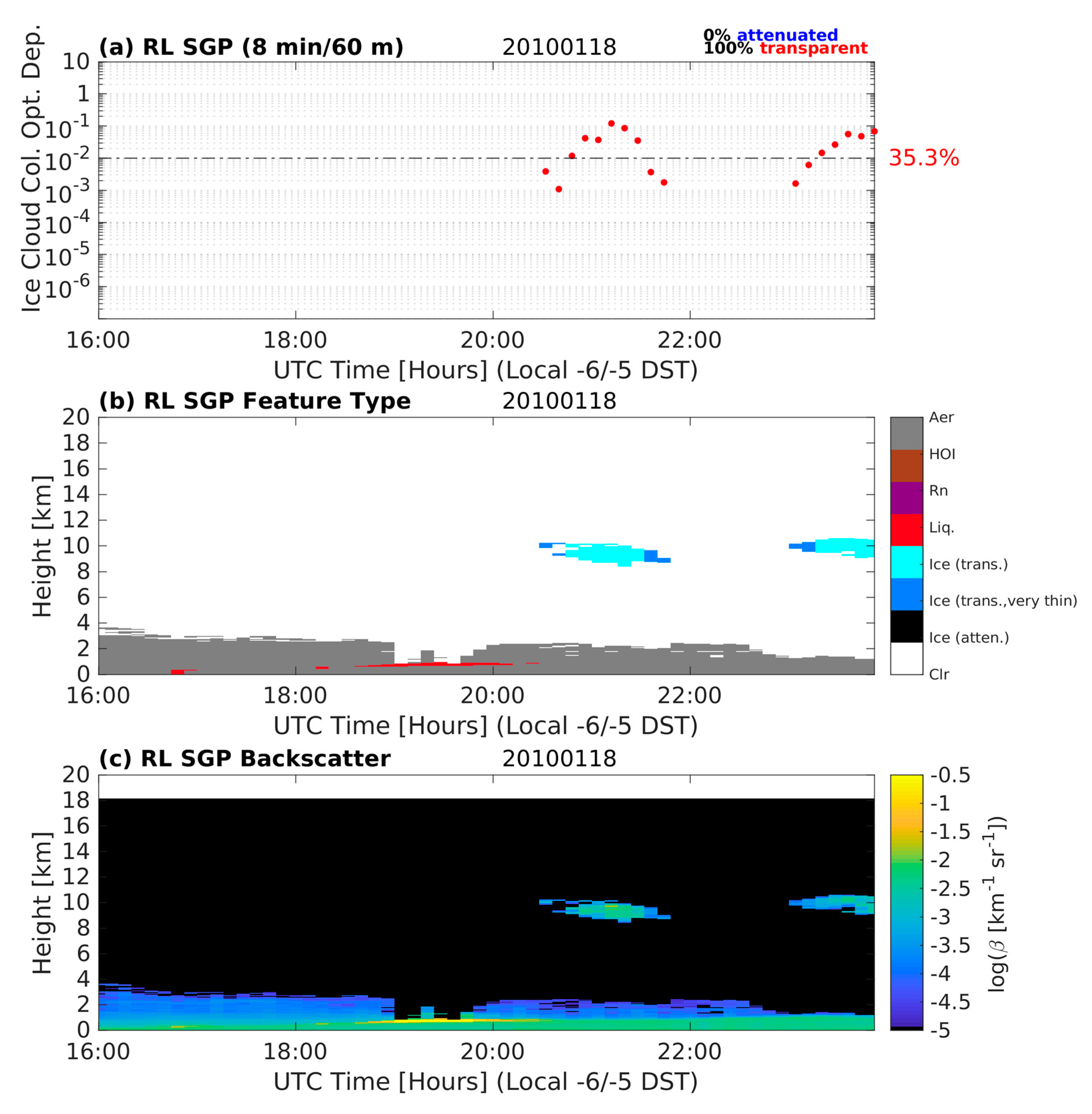
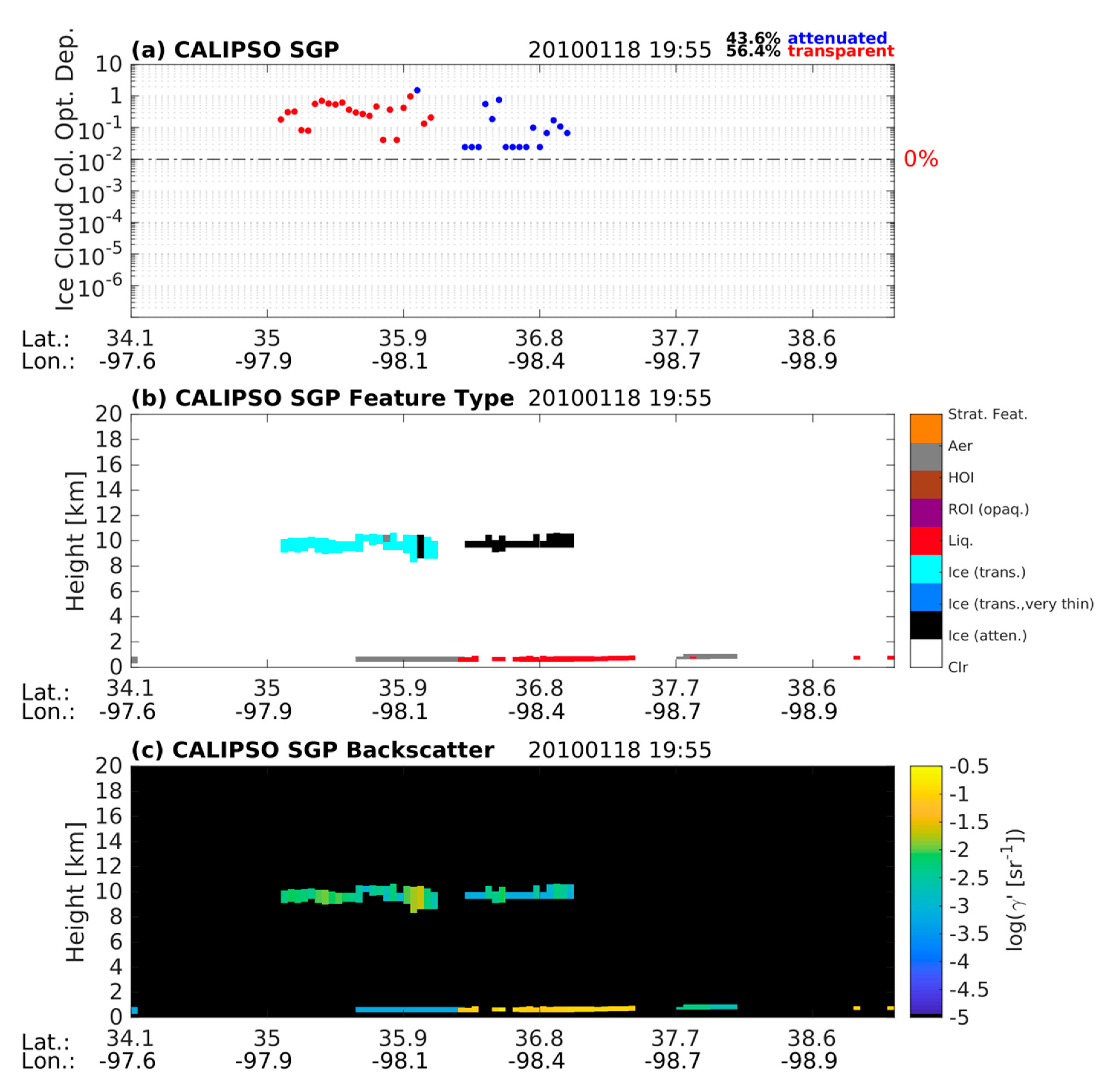
To understand how the optically very thin ice clouds manifest themselves for the RL and CALIPSO observations, we first show a collocated section case, which allows a comparison of the time (and space) evolution of ice cloud column optical depth and vertical profiles of features, including those other than transparent ice clouds. The case is for the collocated section on 18 January 2010 with the RL observations in Figure 1 and CALIPSO observations in Figure 2. CALIPSO passed near the SGP site at around 20:00 UTC. The ice cloud column optical depth for all profiles (including attenuated profiles) are plotted versus time for the RL and versus latitude/longitude for CALIPSO. All feature types detected, including aerosols and liquid clouds, are plotted by time (latitude/longitude) and height for the RL (CALIPSO). The corresponding backscatter is also plotted for all features detected in terms of particulate backscatter for the RL and layer-integrated attenuated backscatter for CALIPSO.
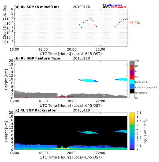
Figure 1.
Raman lidar (RL) retrievals on 18 January 2010 at the Southern Great Plains (SGP) site for collocated profiles with Cloud-Aerosol Lidar and Infrared Pathfinder Satellite Observations (CALIPSO) (±4 h). (a) Ice cloud column optical depths for transparent profiles (red) and attenuated profiles (blue) versus time in UTC. The optically very thin ice cloud threshold ( 0.01) is denoted by the dot-dashed black line. The percentage of transparent ice cloud column optical depths below this threshold compared to all transparent ice cloud column optical depths for this collocated section is labeled to the right of the graph. The percentage of ice cloudy profiles that are transparent and attenuated are given above the graph to the right. (b) Feature classification as either liquid cloud (red), rain (purple), horizontally-oriented ice (HOI; brown), aerosol (gray), transparent ice clouds with 0.01 (light blue), transparent ice clouds with 0.01 (dark blue) or attenuated ice clouds (black). (c) Particulate backscatter (, expressed as the log, units: km−1sr−1) for all features detected.

Figure 2.
CALIPSO retrievals on 18 January 2010 over the SGP site for collocated profiles with RL (within 5° latitude by 5° longitude box centered over SGP). (a) Ice cloud column optical depths for transparent profiles (red) and attenuated profiles (blue) versus latitude/longitude. The optically very thin ice cloud threshold ( 0.01) is denoted by the dot-dashed black line. The percentage of transparent ice cloud column optical depths below this threshold compared to all transparent ice cloud column optical depths for this collocated section is labeled to the right of the graph. The percentage of ice cloudy profiles that are transparent and attenuated are given above the graph to the right. (b) Feature classification as either liquid cloud (red), opaque randomly-oriented ice clouds (purple), horizontally-oriented ice (HOI; brown), aerosol (gray), stratospheric feature (orange), transparent ice clouds with 0.01 (light blue), transparent ice clouds with 0.01 (dark blue) or attenuated ice clouds (black). (c) Layer-integrated attenuated backscatter (, expressed as the log, units: sr−1) for all features detected.
The RL profiles reveal the detection of optically very thin ice clouds. The consecutive profiles of small optical depths are directly adjacent to profiles with ice cloud column optical depths exceeding 0.01 and ice cloud-free profiles; i.e., cloud edges. Around 20:30 UTC, the temporal structure of the optical depths indicates a general increase from around 0.001 to 0.1 and then a decrease back to near 0.001. The same structure is observed at around 23:00 UTC with increasing optical depth from below to above the threshold of 0.01. The temporal evolution provides evidence for the clear sky–cloud continuum [46,47]. The continuum suggests that a transition period exists between clear sky and clouds (aerosols) such that typical binary approaches to clear versus cloudy skies do not adequately capture the atmosphere. The high sensitivity of the RL to detect optically very thin ice clouds provides the capability to observe the clear sky–ice cloud continuum.
The CALIPSO-collocated profiles for this case study do not contain optically very thin ice clouds, although CALIPSO does observe optically very thin ice clouds (Figure 3). Nonetheless, there are ice clouds above lower liquid clouds for attenuated profiles, which may go undetected by a ground-based lidar. This highlights the importance of satellite-based lidars to observe high altitude ice clouds without having to pass through low altitude liquid clouds. Additionally, this highlights the importance of considering transparent profiles when comparing satellite-based and ground-based instruments.
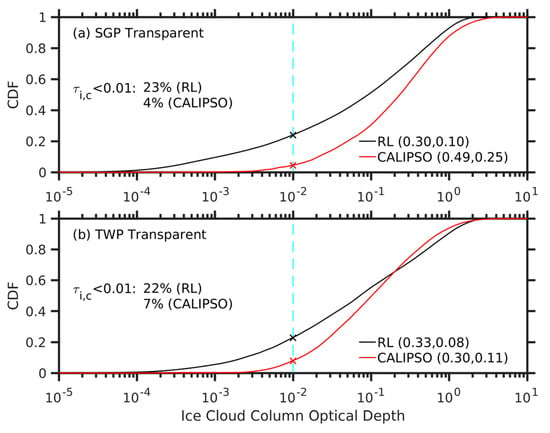
Figure 3.
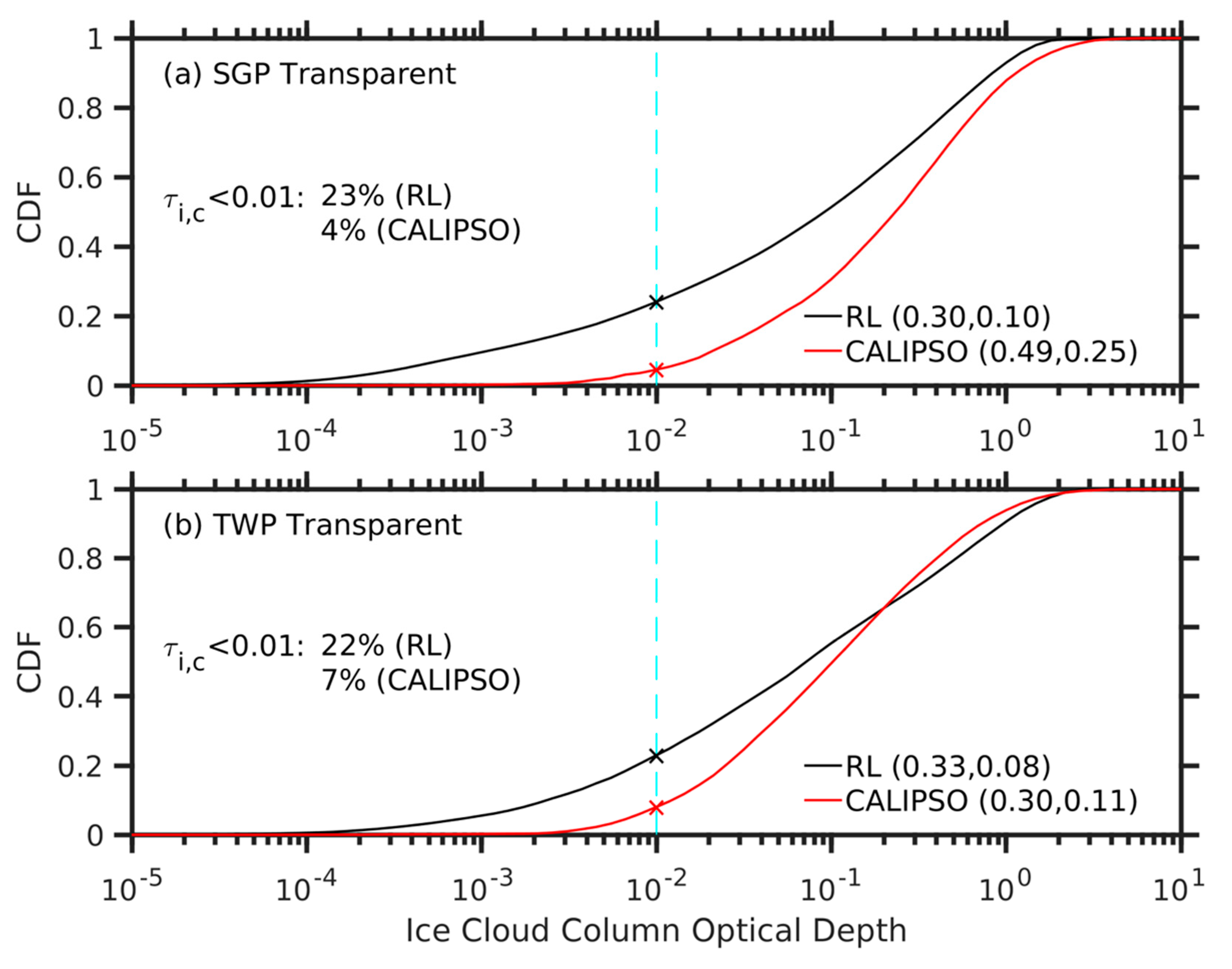
Cumulative distribution functions (CDFs) of ice cloud column optical depths for transparent ice cloud profiles from CALIPSO (red) and RL with CALIPSO-like extinction retrieval resolution (i.e., 8 min/60 m at SGP and 24 min/60 m at the Tropical Western Pacific (TWP) site) (black) for the (a) SGP and the (b) TWP sites. The percentages of the distribution below the ice cloud column optical depth of 0.01 (cyan line) are shown as “x” and the percentage values are given on the left. Mean and median values are given in the parentheses. Data for the RL at the SGP site are from August 2008 to August 2016 and at the TWP site from December 2010 to January 2015. Data for CALIPSO for both the SGP and TWP sites are from June 2006 to August 2016.
3. Methods
To examine the optically very thin ice clouds (τ < 0.01), all transparent profiles from the RLs are considered without discarding profiles when CALIPSO is not passing over. All transparent profiles from the CALIPSO within a 5° latitude by 5° longitude box centered over the SGP and TWP sites are considered without discarding profiles when the RL is not operational. Discarding these profiles produces nearly identical results to those presented here. Overall, the total number of transparent profiles considered are 334,675 for the RL over SGP, 100,640 for CALIPSO over SGP, 25,958 for the RL over TWP and 100,652 for CALIPSO over TWP in this analysis (see Table 1).

Table 1.
Number of total available profiles, transparent profiles, and transparent ice cloud profiles (i.e., transparent profiles where ice clouds are detected) for the RL and CALIPSO at the SGP and TWP sites. For the transparent ice cloud profiles, the number of profiles with ice cloud column optical depths greater than 0 (i.e., all transparent ice cloud profiles), less than 0.01, less than 0.005 and less than 0.001 are given. The numbers in the parentheses are the fraction relative to the number of all transparent ice cloud profiles. Data for the RL at the SGP site are from August 2008 to August 2016 and at the TWP site from December 2010 to January 2015. Data for CALIPSO for both the SGP and TWP sites are from June 2006 to August 2016.
Ice cloud column optical depths are constructed as integrating all ice cloud particulate extinction within a profile, expressed as
where is the ice cloud column optical depth, is ice cloud particulate extinction in km−1, and ztop (zbase) is the highest (lowest) ice cloud top (base) height of the atmospheric profile.
Ice clouds with column optical depths below 0.01 are analyzed to determine the nearby profile conditions. For all transparent ice cloud profiles with ice cloud column optical depths below 0.01, the consecutive profiles are grouped, and the profiles directly preceding and succeeding the group in time/space are checked. If the ice cloud column optical depth is above 0.01 for either the preceding or succeeding profile, but the profile on the other side is clear sky, this group of optically very thin ice cloud profiles are considered as a “cloud edge.” If both the preceding and succeeding profiles have an ice cloud column optical depth above 0.01, the group of optically very thin ice clouds are considered as “in-between clouds.” If both the preceding and succeeding profiles are clear sky, the group of optically very thin ice clouds are considered as “isolated.” The group that does not belong to the above three categories is not considered here, which are related to the preceding/succeeding profiles that have no measurements or are attenuated. They represent only about 10% of the optically very thin ice cloud profiles from both the RL and CALIPSO.
4. Results
4.1. Ice Cloudy Optical Depth Distribution
Figure 3 shows the cumulative distribution functions (CDFs) of ice cloud column optical depths for transparent profiles when ice clouds are detected for the RL and CALIPSO. The dashed cyan line for = 0.01 highlights the focus of this study on the distribution of transparent ice cloud column optical depths below this threshold. It is seen that at both sites, more than 20% of transparent ice cloud profiles from the RLs have < 0.01, but only a few percent of those from CALIPSO have < 0.01. The RL observes more transparent ice cloud column optical depths below 0.01 than CALIPSO at both SGP and TWP, indicating the higher sensitivity of the RL in comparison to CALIPSO. In Figure 3, the percentages of the transparent profiles from the RLs and CALIPSO are not forced to be the same. By using consistent resolutions between the RL and CALIPSO and noting a small effect of the transparent definitions, the differences in the CDFs between the RL and CALIPSO are mainly related to the differences in instrument sensitivity [8]. The different lidar ratios used also play a role in these differences. Considering transparent profiles that are not necessarily temporally collocated might also contribute. Table 1 lists the number of profiles for all time, transparent, ice cloud transparent, and ice cloud transparent with ice cloud column optical depths below 0.01, 0.005, and 0.001 for the RLs and CALIPSO at SGP and TWP. The RL always observes more profiles of optically very thin ice clouds relative to total ice cloud transparent profiles in comparison to CALIPSO.
4.2. Optically Very Thin Ice Clouds Adjacent Profiles
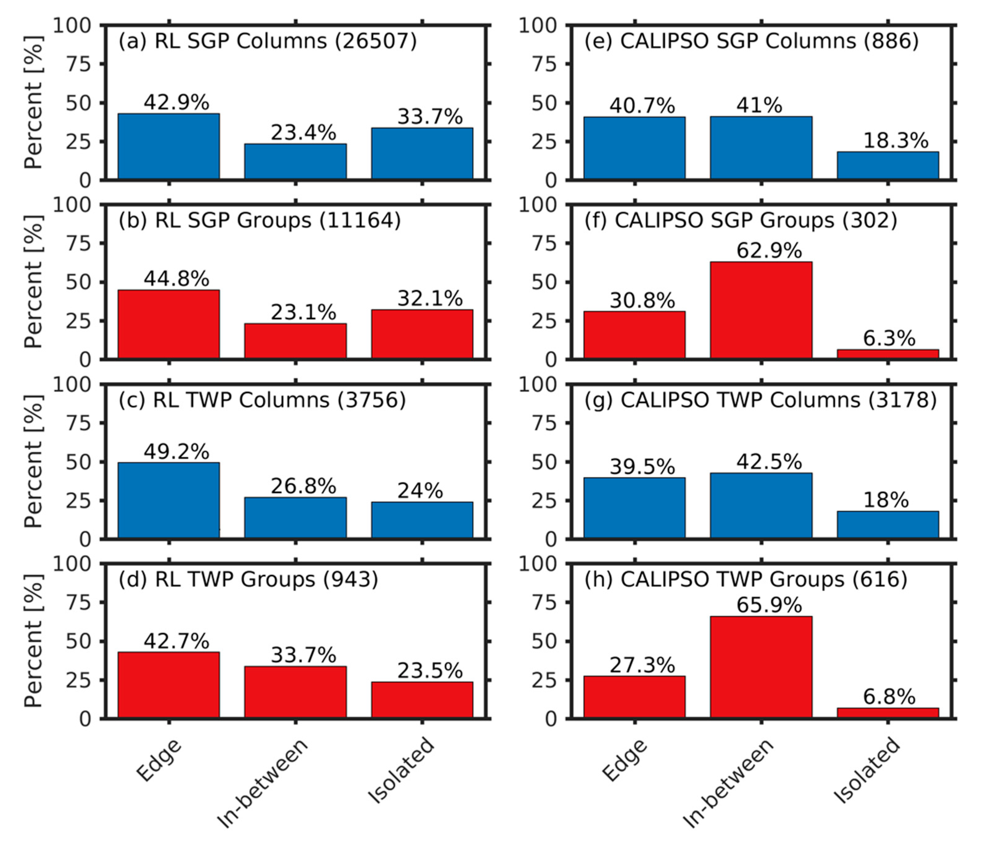
Figure 4 shows the percentage breakdown of transparent ice cloud profiles with ice cloud column optical depths below 0.01 separated into cloud edge, in-between clouds or isolated based on the immediately adjacent profiles for the RL and CALIPSO. The percentage breakdown is constructed for the number of columns in each category counted individually as well as the number of groups of continuous profiles of transparent ice cloud column optical depth below 0.01. For example, if 5 consecutive profiles of ice cloud column optical depths below 0.01 are preceded by a clear-sky profile and succeeded by an ice cloud column optical depth greater than 0.01, the column count for edge would increase by 5 and the group count for edge would increase by 1. The motivation to separate the analysis into columns and groups is for continuous columns to be counted both individually and as a single group because the continuous columns stem from the same time and atmospheric state.
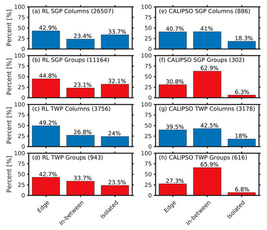
Figure 4.
Percentage breakdown of the transparent ice cloud profiles with ice cloud column optical depths below 0.01 into “edge”, “in-between” and “isolated” for the RL (left) and CALIPSO (right) at the SGP (top two) and TWP (bottom two) sites. “Edge” refers to one of the adjacent profiles with an ice cloud column optical depth above 0.01 and where the other adjacent profile is clear sky. “In-between” refers to both of the adjacent profiles with an ice cloud column optical depth above 0.01. “Isolated” refers to both of the adjacent profiles being clear sky. The percentage breakdown is considered for columns (blue) and groups (red), where columns count all transparent ice cloud profiles with ice cloud column optical depths below 0.01 equally and groups count consecutive transparent ice cloud profiles with ice cloud column optical depths below 0.01 as one group. The total number of samples for each panel is given in the parentheses. Data for the RL at the SGP site are from August 2008 to August 2016 and at the TWP site from December 2010 to January 2015. Data for CALIPSO for both the SGP and TWP site are from June 2006 to August 2016.
For the RL, the cloud edge category has the largest percentage of transparent ice cloud profiles with ice cloud column optical depths below 0.01 over both SGP (~44%) and TWP (~47%) regardless of columns or groups. When combining together the percentages for cloud edge and in-between columns, 66% and 76% of the optically very thin ice clouds are adjacent to optically thicker ice clouds at SGP and TWP, respectively. For the RL, the breakdown percentage is similar in terms of columns and groups. The large percentage of optically very thin ice clouds nearby optically thicker ice clouds provides confidence that the small optical depths are real phenomena and not noise (i.e., false positives). For the isolated category, about 10% more optically very thin ice clouds are observed at SGP than at TWP relative to the total number of optically very thin ice clouds observed. The difference is possibly related to differences between mid-latitude (i.e., SGP) and tropical (i.e., TWP) ice clouds, such as in their formation or horizontal extent (Section 4.3).
For CALIPSO, the cloud edge category is largest for columns but the in-between category is largest for groups for both SGP and TWP. Similar to the RL, combining the cloud edge and in-between percentages together yields 82% over both SGP and TWP, indicating that the vast majority of optically very thin ice clouds are directly next to optically thicker ice clouds. The in-between percentage is larger compared to the RL at the expense of a smaller percentage for the cloud edge.
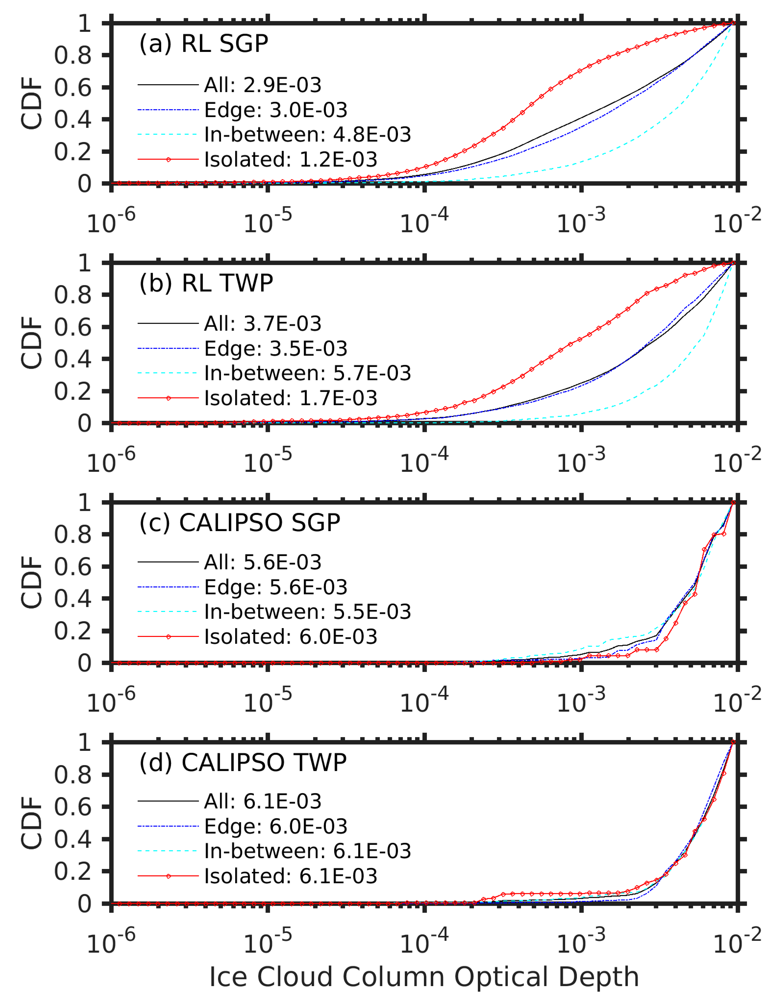
Figure 5 shows the CDFs for transparent ice cloud column optical depths below 0.01 as well as the CDFs for those associated with cloud edge, in between clouds and isolated for the RL and CALIPSO. The RL distributions indicate that isolated optically very thin ice clouds contain the thinnest optical depths, which is also supported by the smallest mean optical depth. In-between clouds have the largest optical depths and highest mean optical depth, unsurprisingly, given the larger optical depths of both the preceding and succeeding profile. The distribution for cloud edges is in the middle in terms of the mean and CDF. The cloud edge’s CDF closely follows the total distribution of transparent ice cloud column optical depths below 0.01. In contrast to the RL, CALIPSO’s distributions and means are nearly identical for cloud edge, in-between clouds and isolated. This suggests that the smaller optical depths only observed by the higher sensitivity RL contribute to the different distributions and means between cloud edge, in-between clouds and isolated clouds.
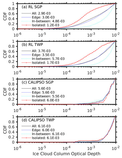
Figure 5.
Cumulative distribution functions (CDFs) of ice cloud column optical depths below 0.01 (solid black) as well as those separated into 3 categories: cloud edges (dot dashed dark blue), in-between (dashed light blue) and isolated (circle red) for (a) RL SGP, (b) RL TWP, (c) CALIPSO SGP and (d) CALIPSO TWP. Mean values are given. Data for the RL at the SGP site are from August 2008 to August 2016 and at the TWP site from December 2010 to January 2015. Data for CALIPSO for both the SGP and TWP site are from June 2006 to August 2016.
4.3. Optically Very Thin Ice Clouds Horizontal Extent
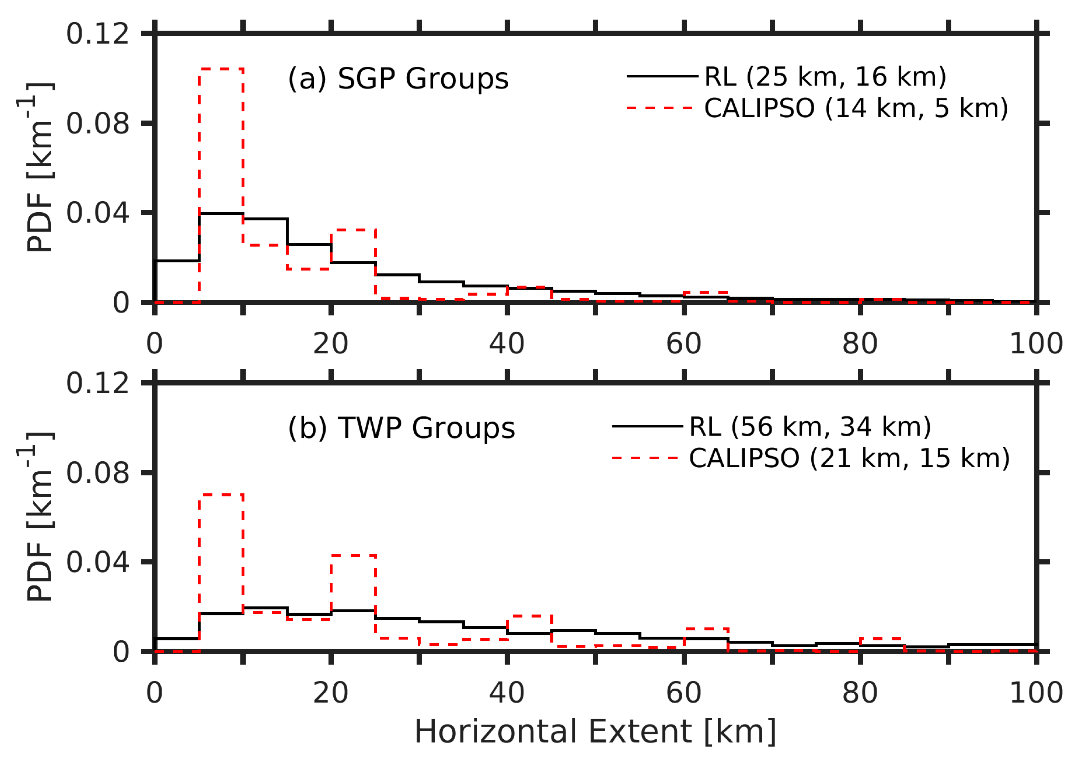
In addition to understanding how the optically very thin ice clouds reveal themselves temporally in the observations (see the Case Study), the horizontal extent of the optically very thin ice clouds is also of interest. The horizontal extent of these clouds and ice clouds more broadly are necessary to improve projections of climatic effects [48]. For the RL, the temporal extent of the optically very thin ice clouds can be translated into the horizontal extent by incorporating the winds from nearby radiosondes. For each transparent profile with an ice cloud column optical depth below 0.01, the closest radiosonde to the profile’s time is found and the wind speed is matched by height for all ice clouds observed in the profile. The wind speed is multiplied by the time step (i.e., 8 min for SGP and 24 min for TWP) to yield a horizontal distance. The column horizontal extent is then determined as the mean horizontal distance of ice clouds observed within the profile. The group horizontal extent is therefore the sum of the column horizontal extent in a group of optically very thin ice clouds (i.e., continuous transparent ice cloud profiles of optically very thin ice clouds, identical to that defined in Figure 4). For CALIPSO, the horizontal extent can be calculated by summing the number of 5 km profiles for each group of optically very thin ice clouds.
Figure 6 shows the probability distribution functions (PDF) of horizontal extent for optically very thin ice cloud groups observed by the RL and CALIPSO. CALIPSO observes a smaller mean and median horizontal extent compared to the RL over both SGP and TWP. This aligns with the observation that the higher sensitivity RL observes more optically very thin ice clouds. Therefore, the RL likely observes more of the tail end of a group of optically very thin ice clouds compared to CALIPSO, which would increase the horizontal extent observed overall and result in a higher mean and median horizontal extent for the RL. The distinct peaks in the CALIPSO PDFs are the result of CALIPSO’s retrieval scheme. CALIPSO retrieves optical depths for clouds detected at horizontal averaging distances of 5 km, 20 km and 80 km [44]. Therefore, the peaks correspond to these horizontal averaging distances and any combination of the horizontal averaging distances.
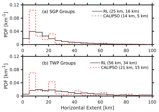
Figure 6.
Probability distribution functions (PDFs) of the horizontal extent for groups of continuous transparent ice cloud profiles of ice cloud column optical depths below 0.01 for the RL (solid black) and CALIPSO (dashed red) over the (a) SGP and (b) TWP sites. Mean and median values are given in the parentheses. Data for the RL at the SGP site are from August 2008 to August 2016 and at the TWP site from December 2010 to January 2015. Data for CALIPSO for both the SGP and TWP site are from June 2006 to August 2016.
4.4. Optically Very Thin Ice Cloud Vertical Occurrence
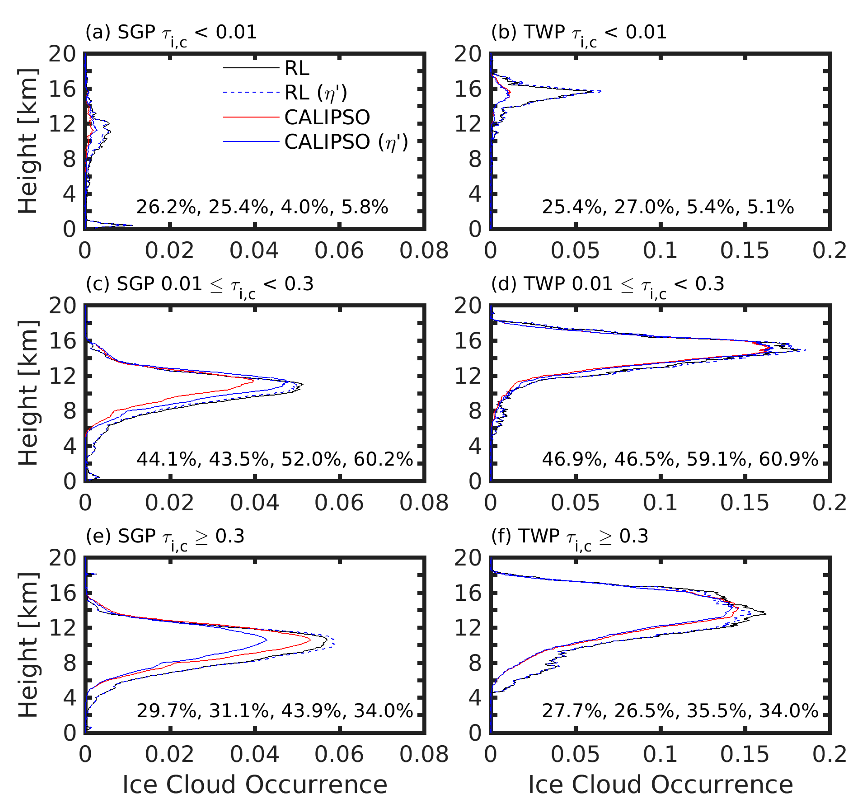
In addition to how often optically very thin ice clouds occur, information on the vertical distribution in the atmosphere is another key component to determine the ice cloud radiative effects [49]. Figure 7 shows the ice cloud occurrence with height for the RL with CALIPSO-like extinction resolution and CALIPSO, separated into optically very thin ( 0.01), thin (0.01 0.3) and relatively thick ( 0.3) ice clouds. Collocated profiles where the transparent percentages are matched between the RL and CALIPSO are used (Section 2.3). The vertical ice cloud occurrence separated into optical depth ranges are also plotted for the RL and CALIPSO using a lidar ratio from the CALIPSO temperature-dependent effective lidar ratio parameterization [45] divided by a constant multiple scattering factor of 0.8 for SGP and 0.7 for TWP. This is the case that leads to a lidar ratio used for both the RL and CALIPSO, which is consistent with the RL’s directly retrieved lidar ratios and CALIPSO’s constrained retrievals of effective lidar ratios [8]. These factors (i.e., matching resolution, lidar ratio, and transparent percentages) are considered to ensure a fair comparison, which are among the factors that were used to reconcile ice cloud column optical depths between the RL and CALIPSO [8]. The only factor that is not considered is the higher sensitivity of the RL (i.e., larger cloud fraction), which is largely isolated in this comparison. The differences caused by the RL’s higher sensitivity are examined by looking at where the optically very thin ice clouds vertically occur by comparing the solid blue and dashed-blue lines in Figure 7.
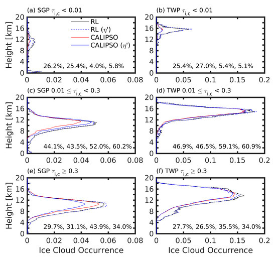
Figure 7.
Ice cloud occurrence profiles from CALIPSO (solid red) and the RL with CALIPSO-like extinction resolution (i.e., 8 min/60 m at SGP and 24 min/60 m at TWP) using the best-estimate lidar ratio (solid black) for < 0.01 (top), 0.01 ≤ < 0.3 (middle), and ≥ 0.3 (bottom) over SGP (left) and TWP (right). Also plotted are ice cloud occurrence profiles with lidar ratios determined by the CALIPSO’s Version 4 temperature-dependent effective lidar ratio parameterization divided by a constant multiple scattering factor of 0.8 for SGP and 0.7 for TWP for CALIPSO (blue) and the RL (dashed blue). Only considered are transparent collocated profiles by matching the percentage of transparent profiles from the RL and CALIPSO. Percentage of the distribution represented in each optical depth range are given for the RL, RL with matching lidar ratio between the RL and CALIPSO, CALIPSO and CALIPSO with matching lidar ratio between the RL and CALIPSO. Data are for times collocated between the RL and CALIPSO at the SGP site from August 2008 to August 2016 and the TWP site from December 2010 to January 2015.
For the thin and relatively thick ice clouds, the RL and CALIPSO largely agree, except over SGP for 0.3. The RL observes slightly more thick ice clouds than CALIPSO. As noted in Figure 3, the RL observes more optically very thin ice clouds at both SGP and TWP. These ice clouds occur at high altitudes, near the height for maximum occurrence of around 10 km and 15 km at SGP and TWP, respectively. Optically very thin ice clouds also occur around 1 km at SGP. Of all optically very thin ice clouds below 2 km at SGP, nearly all (~99.7%) occur between November and March. The wintertime occurrence suggest these optically very thin ice clouds may be precipitating ice such as snow. Overall, the vertical occurrences of optically very thin ice clouds agree with those for tropical (TWP) and mid-latitude (SGP) subvisual ice clouds as presented in Hong and Liu [25].
4.5. Global Cloud Fraction
The RL with higher sensitivity detects more clouds than CALIPSO. However, the RL is confined to a point-location, whereas CALIPSO provides near-global cloud measurements. The strengths for both instruments offer the ability to infer what the global cloud fraction is by estimating what the cloud fraction undetected by CALIPSO is and comparing that to what CALIPSO observes for the cloud fraction globally. The cloud fraction undetected by CALIPSO is estimated by averaging the difference between the RL and CALIPSO cloud fraction at SGP and TWP. CALIPSO’s global cloud fraction is determined by considering all available CALIPSO profiles for the time period considered (2006–2016).
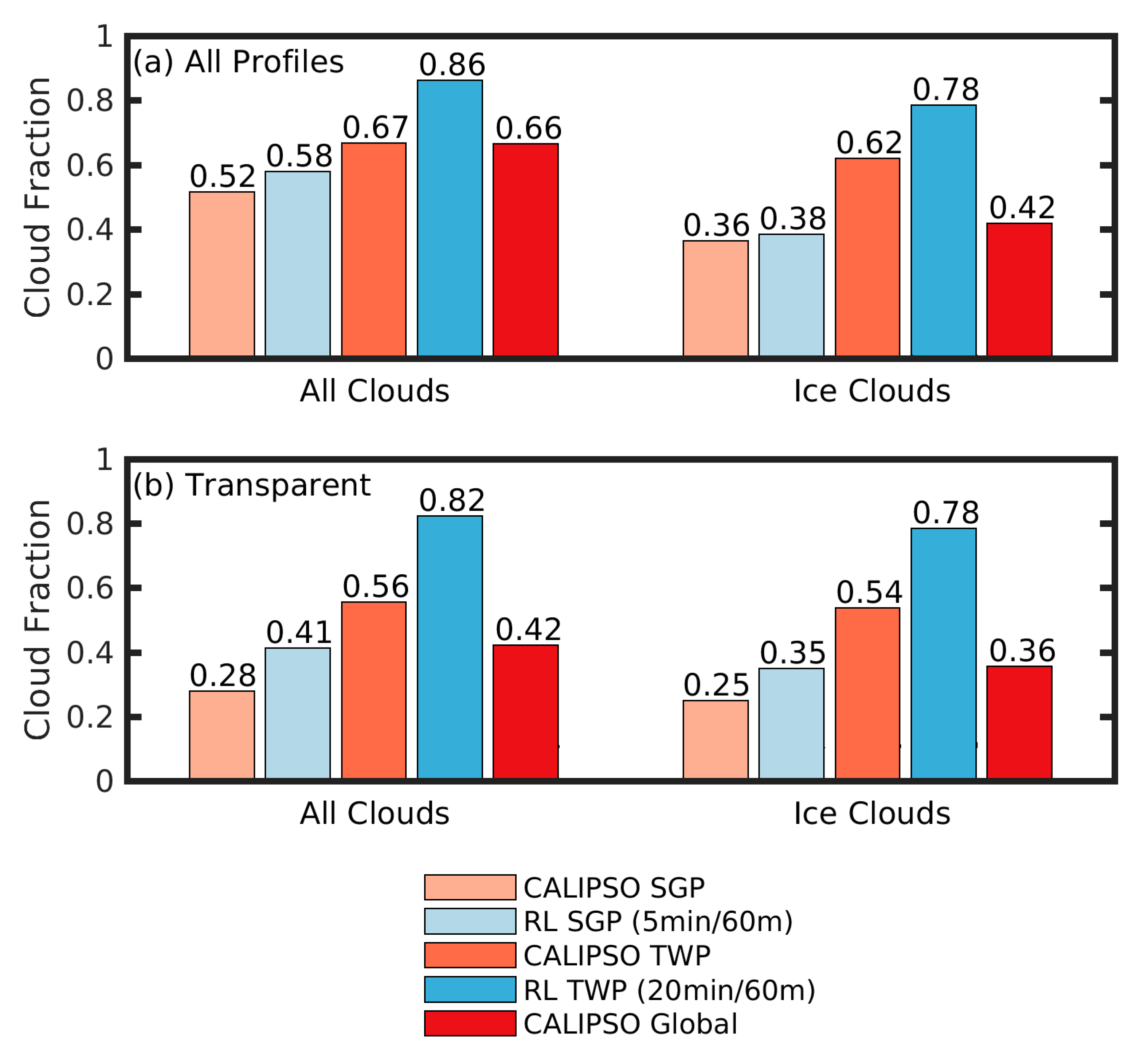
Figure 8 shows the cloud fractions from the RL and CALIPSO over SGP and TWP, and CALIPSO over the globe. Cloud fractions are derived by using all profiles (upper panel) and transparent-only profiles (lower panel) for all clouds (left) and ice clouds (right). Ice clouds are those only containing randomly oriented ice particles. The RL resolution is consistent with CALIPSO’s feature detection (i.e., CALIPSO-like feature detection resolution), which is 5 min/60 m over SGP and 20 min/60 m over TWP [8]. Cloud fractions are constructed by only considering low to high confidence cloud layers. However, the results are nearly identical when including no-confidence cloud layers or when restricting this to medium and high confidence cloud layers, especially for ice clouds.
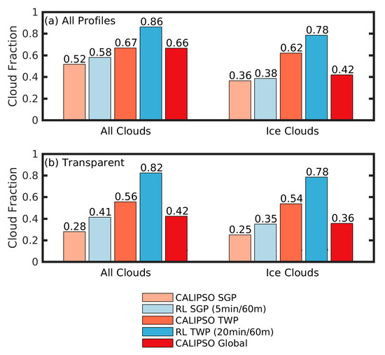
Figure 8.
Cloud fractions of all clouds (left) and ice clouds (right). Cloud fractions are based on (a) all profiles and (b) transparent profiles for CALIPSO (red) and the RL (blue). Cloud fractions are for SGP (light color), TWP (medium color) and CALIPSO global (dark red). The RL resolution is the CALIPSO-like feature detection resolution (i.e., 5 min/60 m at SGP and 20 min/60 m at TWP). Values are also given above the bars. Data for the RL at the SGP site are from August 2008 to August 2016 and at the TWP site from December 2010 to January 2015. Data for CALIPSO are from June 2006 to August 2016.
All clouds from all profiles provide an estimate for the global cloudiness considering all observations. CALIPSO’s global cloud fraction is 0.66 and the average cloud fraction difference between the RL and CALIPSO at SGP and TWP is +0.13. For transparent profiles, the CALIPSO global cloud fraction is 0.42, with the average cloud fraction difference between the RL and CALIPSO at SGP and TWP being +0.20. The difference in the RL and CALIPSO for all cloud fractions are largely caused from the differences in instrument sensitivity: the optically very thin clouds are only detected by the RL.
The results for ice clouds for all profiles (top right in Figure 8) should be interpreted with caution since the CALIPSO, which is in space, samples different ice clouds than the ground-based RL. The case study highlights the differences where CALIPSO observed ice clouds above liquid clouds, which is more challenging to detect by RLs. Ice clouds for transparent profiles afford the ability to estimate what the global cloud fraction might be if CALIPSO detected optically very thin ice clouds which the higher sensitivity RL observes in greater numbers. Globally, CALIPSO observes an ice cloud fraction of 0.36 for transparent profiles, while the average cloud fraction difference between the RL and CALIPSO at SGP and TWP is +0.17.
5. Discussion
The higher sensitivity of the RL allows the opportunity to detect optically very thin ice clouds, which often go undetected by CALIPSO. The optically very thin ice clouds represent a large proportion (22–23%) of ice cloudy profiles. With the focus of this study being on the optically thinnest clouds that can be detected by the instruments, a discussion of the uncertainty in the optical depth retrievals is necessary. The optical depth is derived from the particulate extinction (Equation (1)); therefore, the focus will be on uncertainties in particulate extinction. For both the RL and CALIPSO, uncertainty in particulate extinction arises from uncertainties in the lidar ratio and particulate backscatter, which can be expressed as
where is the uncertainty in the particulate extinction in km−1, is the uncertainty in the lidar ratio in sr, and is the uncertainty in the particulate backscatter in (km sr)−1.
For the RL, the uncertainties for the lidar ratio and particulate backscatter depend on the methods used to determine those quantities. RL lidar ratio and particulate backscatter uncertainties are composed of uncertainties in the signal, overlap function and calibration coefficient. For CALIPSO, the uncertainty for the lidar ratio also depends on the method used to determine the lidar ratio. The lidar ratio uncertainty depends only on the uncertainties in the measured data for constrained retrievals. The lidar ratio uncertainty is assigned a relative uncertainty of 25% for unconstrained retrievals [45]. The uncertainty in particulate backscatter for CALIPSO is composed of the uncertainties in the molecular backscatter, normalization backscatter, molecular transmittance and particulate transmittance [45,50].
To gauge the uncertainties in the ice cloud column optical depth, the absolute uncertainty in particulate extinction is expressed as
where is the absolute uncertainty in the ice cloud column optical depth in km−1, and is the uncertainty in the ice cloud particulate extinction in km−1. This approach of determining the optical depth uncertainty neglects the contribution of the covariance of the lidar ratio and particulate backscatter to the optical depth uncertainty. This contribution, however, is negligible for low optical depths (i.e., the focus of this analysis) with typical SNRs [50]. The median absolute uncertainty for transparent profiles with ice cloud column optical depths below 0.01 is 1.3E−3 km−1 (2.3E−3 km−1) and 5.8E−3 km−1 (4.8E−3 km−1) for the RL and CALIPSO SGP (TWP). The median relative uncertainty (i.e., Equation (3) divided by Equation (1)) for transparent profiles with ice cloud column optical depths below 0.01 is 82.9% (85.2%) and 91.3% (73.1%) for the RL and CALIPSO SGP (TWP), respectively. The relative uncertainty is large, which is the result of summing various factors contributing to ice cloud extinction uncertainties, and is relative to small values by only considering the ice cloud column optical depths below 0.01. For reference, the median absolute uncertainty for all ice cloudy transparent profiles (Figure 3) is 0.029 (0.030) and 0.18 (0.10) for the RL and CALIPSO SGP (TWP), respectively. The median relative uncertainty for all ice cloudy transparent profiles (Figure 3) is 30.3% (33.7%) and 66.8% (72.2%) for the RL and CALIPSO over SGP (TWP), respectively.
Analyzing profiles nearby to the optically very thin ice clouds indicates that optically thicker ice clouds are directly adjacent, categorized as cloud edge or in-between clouds. This provides confidence that the optically very thin ice clouds are real atmospheric phenomena and not artifacts of noise. The optically very thin ice clouds detected by the RL indicate the great value in the RL to observe clouds; in particular, those that prove challenging for remote sensing.
The temporal structure of optically very thin ice clouds observed by the RL reveals a clear sky–cloud continuum that has also been shown for aerosols and low marine clouds [46,47]. The clear sky–cloud continuum drifts away from the binary cloud mask approach as a spectrum exists between clear and cloudy sky.
The optically very thin ice clouds detected by the RL can aid in estimating a global cloud fraction. Leveraging the strengths of the RL and CALIPSO suggests that the cloud fraction could be around 0.13 larger than the CALIPSO global cloud fraction of 0.66 based on the average difference between the RL and CALIPSO at SGP and TWP. This study is also informative of the ice cloud fraction for transparent profiles. For transparent profiles, the ice cloud fraction could be around 0.17 larger than the CALIPSO global ice cloud fraction of 0.36. The possible underestimation is largely related to the optically very thin ice clouds that can go undetected by CALIPSO. Optically thin ice clouds have recently been discovered to be vitally important for understanding ice cloud climatic impacts. Berry and Mace [11] showed that the median ice water path was more important than the mean ice water path (as previously thought) for determining the cloud radiative forcing of ice clouds due to the abundance of optically thin ice clouds which were largely missed by earlier remote sensing efforts. In this study, we have not quantified the possible radiative effects related to the optically very thin ice clouds, although we expect the overall effect to be small. Other recent studies have calculated cloud radiative forcings of ice clouds for varying locations and altitudes [13,14,15,16]. This necessitates comprehensive ice cloud detection and ice cloud optical depth distributions and highlights the importance for understanding optically very thin ice clouds as presented in this study.
6. Summary
Optically very thin ice clouds are analyzed from ground-based Raman lidars (RLs) at the atmospheric radiation measurement (ARM) program Southern Great Plains (SGP) site for 8 years and at the ARM Tropical Western Pacific (TWP) site for 4 years. Also analyzed are optically very thin ice clouds from the space-borne CALIPSO for 10 years at the ARM SGP site, ARM TWP site and globally. The overall occurrence, nearby atmospheric environment, temporal structure, horizontal extent, vertical occurrence and the global cloudiness implications of optically very thin clouds (i.e., ice clouds with ice cloud column optical depth less than 0.01) are investigated.
A case for a collocated section between the RL and CALIPSO was compared for the time (and space) evolution of ice cloud column optical depth and vertical profiles of all features detected. The RL temporal progression of the ice cloud column optical depth revealed a clear sky–cloud continuum that has been previously noted for aerosols and other cloud types [46,47]. The case comparison emphasized the importance of only considering transparent profiles when comparing ground-based and space-based instruments. Additionally, the case study highlighted the importance for space-based lidars to observe ice clouds above liquid clouds as well as the importance of ground-based instruments with higher sensitivity to detect optically very thin ice clouds.
CALIPSO was shown to detect significantly fewer ice clouds than the RL, particularly, optically very thin ice clouds, when considering transparent profiles. Transparent optically very thin ice clouds are separated into 3 categories based on the preceding and succeeding profiles: “cloud edge”, “in-between” and “isolated”. RL and CALIPSO observations both indicate that a majority of optically very thin ice clouds are directly adjacent to optically thicker ice clouds. CDFs of ice cloud optical depth for optically very thin ice clouds showed that the mean and distributions were lowest for “isolated”, highest for “in-between” and closely followed by the total optically very thin ice cloud distribution for “cloud edges” from the RL. CALIPSO indicated little difference between the 3 categories in terms of means and distribution.
The horizontal extent of the optically very thin ice clouds for both the RL and CALIPSO was calculated. The mean horizontal extent for all optically very thin ice cloud groups observed by the RL (CALIPSO) is 25 (14) km and 56 (21) km for SGP and TWP, respectively. The smaller horizontal extent for CALIPSO compared to the RL aligns with the higher sensitivity RL observing smaller optical depths.
The vertical occurrence of optically very thin, thin (0.01 0.3) and relatively thick ( 0.3) ice clouds was compared for collocated profiles where the transparent percentages were matched between the RL and CALIPSO. The optically thin and thick ice clouds reasonably agreed when the resolution and lidar ratio were also consistent. The optically very thin ice clouds disagreed near the height of maximum ice cloud occurrence of 10 km and 15 km for SGP and TWP, respectively. Additionally, disagreement was found around 1 km at SGP.
Global cloudiness was estimated from the RL and CALIPSO observations. All clouds for all profiles considered indicate an average cloud fraction difference between the RL and CALIPSO at SGP and TWP of +0.13 and a CALIPSO global cloud fraction of 0.66. Ice clouds for transparent profiles estimate an average cloud fraction difference of +0.17 between the the RL and CALIPSO at SGP and TWP with a CALIPSO global cloud fraction of 0.36.
This study shows that optically very thin ice clouds are prevalent and may increase the global cloud fraction estimate from those derived from satellite-based instruments. Higher-sensitivity ground-based instruments provide measurements of optically very thin ice clouds undetected by space-based instruments. Space-based instruments provide global spatial coverage unparalleled by ground-based instruments. Leveraging the strengths of ground-based and space-based instruments provides a more comprehensive knowledge of ice cloud distribution spatially and optically, with the ability to better understand ice cloud radiative effects.
Author Contributions
K.A.B and Q.F. conceived and designed the analysis; K.A.B. performed the analysis; K.A.B. and Q.F. analyzed the results and wrote the paper.
Funding
This research was funded by the Office of Science (BER), U.S. Department of Energy under Grant DE-SC0018190, and by NASA Grants 80NSSC18K1031 and NNX16AO95G.
Acknowledgments
The Raman lidar RL-FEX can be download from the ARM data archive (www.arm.gov/data) as an evaluation value-added product (VAP). The CALIPSO data sets were downloaded from the NASA Langley Research Center Atmospheric Science Data Center (www.eosweb.larc.nasa.gov/project/calipso/calipso_table). We thank J.R. Campbell for helpful suggestions and encouragement of this work. We also thank two anonymous reviewers for providing reviews that improved this study.
Conflicts of Interest
The authors declare no conflict of interest.
References
- Liou, K.-N. Influence of Cirrus Clouds on Weather and Climate Processes: A Global Perspective. Mon. Weather Rev. 1986, 114, 1167–1199. [Google Scholar] [CrossRef]
- Sassen, K.; Campbell, J.R. A Midlatitude Cirrus Cloud Climatology from the Facility for Atmospheric Remote Sensing. Part I: Macrophysical and Synoptic Properties. J. Atmos. Sci. 2001, 58, 481–496. [Google Scholar] [CrossRef]
- Fu, Q.; Hu, Y.; Yang, Q. Identifying the top of the tropical tropopause layer from vertical mass flux analysis and CALIPSO lidar cloud observations. Geophys. Res. Lett. 2007, 34, L14813. [Google Scholar] [CrossRef]
- Holz, R.E.; Ackerman, S.A.; Nagle, F.W.; Frey, R.; Dutcher, S.; Kuehn, R.E.; Vaughan, M.A.; Baum, B. Global Moderate Resolution Imaging Spectroradiometer (MODIS) cloud detection and height evaluation using CALIOP. J. Geophys. Res. 2008, 113, D00A19. [Google Scholar] [CrossRef]
- Mace, G.G.; Zhang, Q.; Vaughan, M.; Marchand, R.; Stephens, G.; Trepte, C.; Winker, D. A description of hydrometeor layer occurrence statistics derived from the first year of merged Cloudsat and CALIPSO data. J. Geophys. Res. 2009, 114, D00A26. [Google Scholar] [CrossRef]
- Yang, Q.; Fu, Q.; Hu, Y. Radiative impacts of clouds in the tropical tropopause layer. J. Geophys. Res. 2010, 115, D00H12. [Google Scholar] [CrossRef]
- Thorsen, T.J.; Fu, Q.; Comstock, J. Comparison of the CALIPSO satellite and ground-based observations of cirrus clouds at the ARM TWP sites. J. Geophys. Res. Atmos. 2011, 116. [Google Scholar] [CrossRef]
- Balmes, K.A.; Fu, Q.; Thorsen, T.J. Differences in Ice Cloud Optical Depth from CALIPSO and Ground-Based Raman Lidar at the ARM SGP and TWP Sites. J. Geophys. Res. Atmos. 2018. under review. [Google Scholar]
- Fu, Q.; Baker, M.; Hartmann, D.L. Atmospheric Chemistry and Physics Tropical cirrus and water vapor: An effective Earth infrared iris feedback? Atmos. Chem. Phys. 2002, 2, 31–37. [Google Scholar] [CrossRef]
- Lin, L.; Fu, Q.; Zhang, H.; Su, J.; Yang, Q.; Sun, Z. Upward mass fluxes in tropical upper troposphere and lower stratosphere derived from radiative transfer calculations. J. Quant. Spectrosc. Radiat. Transf. 2013, 117, 114–122. [Google Scholar] [CrossRef]
- Berry, E.; Mace, G.G. Cloud properties and radiative effects of the Asian summer monsoon derived from A-Train data. J. Geophys. Res. Atmos. 2014, 119, 9492–9508. [Google Scholar] [CrossRef]
- Sun, W.; Videen, G.; Kato, S.; Lin, B.; Lukashin, C.; Hu, Y. A study of subvisual clouds and their radiation effect with a synergy of CERES, MODIS, CALIPSO, and AIRS data. J. Geophys. Res. Atmos. 2011, 116. [Google Scholar] [CrossRef]
- Bourgeois, Q.; Ekman, A.M.L.; Igel, M.R.; Krejci, R. Ubiquity and impact of thin mid-level clouds in the tropics. Nat. Commun. 2016, 7, 12432. [Google Scholar] [CrossRef] [PubMed]
- Campbell, J.R.; Lolli, S.; Lewis, J.R.; Gu, Y.; Welton, E.J. Daytime Cirrus Cloud Top-of-the-Atmosphere Radiative Forcing Properties at a Midlatitude Site and Their Global Consequences. J. Appl. Meteorol. Climatol. 2016, 55, 1667–1679. [Google Scholar] [CrossRef]
- Kayetha, V.K.; Collins, R.L. Optically thin midlevel ice clouds derived from Cloud Aerosol Lidar and Infrared Pathfinder Satellite Observations. J. Appl. Remote Sens. 2016, 10, 46007. [Google Scholar] [CrossRef]
- Lolli, S.; Campbell, J.R.; Lewis, J.R.; Gu, Y.; Marquis, J.W.; Chew, B.N.; Liew, S.-C.; Salinas, S.V.; Welton, E.J. Daytime Top-of-the-Atmosphere Cirrus Cloud Radiative Forcing Properties at Singapore. J. Appl. Meteorol. Climatol. 2017, 56, 1249–1257. [Google Scholar] [CrossRef]
- Fu, Q.; Smith, M.; Yang, Q. The Impact of Cloud Radiative Effects on the Tropical Tropopause Layer Temperatures. Atmosphere 2018, 9, 377. [Google Scholar] [CrossRef]
- Fueglistaler, S.; Dessler, A.E.; Dunkerton, T.J.; Folkins, I.; Fu, Q.; Mote, P.W. Tropical tropopause layer. Rev. Geophys. 2009, 47, RG1004. [Google Scholar] [CrossRef]
- Winker, D.M.; Pelon, J.; Coakley, J.A.; Ackerman, S.A.; Charlson, R.J.; Colarco, P.R.; Flamant, P.; Fu, Q.; Hoff, R.M.; Kittaka, C.; et al. The CALIPSO Mission: A Global 3D View of Aerosols and Clouds. Bull. Am. Meteorol. Soc. 2010, 91, 1211–1229. [Google Scholar] [CrossRef]
- Sassen, K.; Wang, Z.; Liu, D. Global distribution of cirrus clouds from CloudSat/Cloud-Aerosol Lidar and Infrared Pathfinder Satellite Observations (CALIPSO) measurements. J. Geophys. Res. 2008, 113, D00A12. [Google Scholar] [CrossRef]
- Nazaryan, H.; McCormick, M.P.; Menzel, W.P. Global characterization of cirrus clouds using CALIPSO data. J. Geophys. Res. 2008, 113, D16211. [Google Scholar] [CrossRef]
- Virts, K.S.; Wallace, J.M.; Fu, Q.; Ackerman, T.P. Tropical Tropopause Transition Layer Cirrus as Represented by CALIPSO Lidar Observations. J. Atmos. Sci. 2010, 67, 3113–3129. [Google Scholar] [CrossRef]
- Yoshida, R.; Okamoto, H.; Hagihara, Y.; Ishimoto, H. Global analysis of cloud phase and ice crystal orientation from Cloud-Aerosol Lidar and Infrared Pathfinder Satellite Observation (CALIPSO) data using attenuated backscattering and depolarization ratio. J. Geophys. Res. 2010, 115, D00H32. [Google Scholar] [CrossRef]
- Fu, Q. Bottom up in the tropics. Nat. Clim. Chang. 2013, 3, 957–958. [Google Scholar] [CrossRef]
- Hong, Y.; Liu, G. The Characteristics of Ice Cloud Properties Derived from CloudSat and CALIPSO Measurements. J. Clim. 2015, 28, 3880–3901. [Google Scholar] [CrossRef]
- Tseng, H.-H.; Fu, Q. Tropical tropopause layer cirrus and its relation to tropopause. J. Quant. Spectrosc. Radiat. Transf. 2017, 188, 118–131. [Google Scholar] [CrossRef]
- Tseng, H.-H.; Fu, Q. Temperature Control of the Variability of Tropical Tropopause Layer Cirrus Clouds. J. Geophys. Res. Atmos. 2017, 122, 11062–11075. [Google Scholar] [CrossRef]
- Comstock, J.M.; Ackerman, T.P.; Mace, G.G. Ground-based lidar and radar remote sensing of tropical cirrus clouds at Nauru Island: Cloud statistics and radiative impacts. J. Geophys. Res. Atmos. 2002, 107, AAC 16-1–AAC 16-14. [Google Scholar] [CrossRef]
- Ackerman, S.A.; Holz, R.E.; Frey, R.; Eloranta, E.W.; Maddux, B.C.; McGill, M. Cloud Detection with MODIS. Part II: Validation. J. Atmos. Ocean. Technol. 2008, 25, 1073–1086. [Google Scholar] [CrossRef]
- Grenier, P.; Blanchet, J.; Muñoz-Alpizar, R. Study of polar thin ice clouds and aerosols seen by CloudSat and CALIPSO during midwinter 2007. J. Geophys. Res. 2009, 114, D09201. [Google Scholar] [CrossRef]
- Devasthale, A.; Tjernström, M.; Karlsson, K.-G.; Thomas, M.A.; Jones, C.; Sedlar, J.; Omar, A.H. The vertical distribution of thin features over the Arctic analysed from CALIPSO observations. Tellus B Chem. Phys. Meteorol. 2011, 63, 77–85. [Google Scholar] [CrossRef]
- Sassen, K.; Cho, B.S. Subvisual-Thin Cirrus Lidar Dataset for Satellite Verification and Climatological Research. J. Appl. Meteorol. 1992, 31, 1275–1285. [Google Scholar] [CrossRef]
- Davis, S.; Hlavka, D.; Jensen, E.; Rosenlof, K.; Yang, Q.; Schmidt, S.; Borrmann, S.; Frey, W.; Lawson, P.; Voemel, H.; et al. In situ and lidar observations of tropopause subvisible cirrus clouds during TC4. J. Geophys. Res. 2010, 115, D00J17. [Google Scholar] [CrossRef]
- Thorsen, T.J.; Fu, Q. CALIPSO-inferred aerosol direct radiative effects: Bias estimates using ground-based Raman lidars. J. Geophys. Res. Atmos. 2015, 120, 12209–12220. [Google Scholar] [CrossRef]
- Thorsen, T.J.; Ferrare, R.A.; Hostetler, C.A.; Vaughan, M.A.; Fu, Q. The impact of lidar detection sensitivity on assessing aerosol direct radiative effects. Geophys. Res. Lett. 2017, 44, 9059–9067. [Google Scholar] [CrossRef]
- Ackerman, T.P.; Stokes, G.M. The Atmospheric Radiation Measurement Program. Phys. Today 2003, 56, 38–44. [Google Scholar] [CrossRef]
- Thorsen, T.J.; Fu, Q.; Comstock, J.M.; Sivaraman, C.; Vaughan, M.A.; Winker, D.M.; Turner, D.D. Macrophysical properties of tropical cirrus clouds from the CALIPSO satellite and from ground-based micropulse and Raman lidars. J. Geophys. Res. Atmos. 2013, 118, 9209–9220. [Google Scholar] [CrossRef]
- Thorsen, T.J.; Fu, Q.; Newsom, R.K.; Turner, D.D.; Comstock, J.M. Automated Retrieval of Cloud and Aerosol Properties from the ARM Raman Lidar. Part I: Feature Detection. J. Atmos. Ocean. Technol. 2015, 32, 1977–1998. [Google Scholar] [CrossRef]
- Thorsen, T.J.; Fu, Q. Automated Retrieval of Cloud and Aerosol Properties from the ARM Raman Lidar. Part II: Extinction. J. Atmos. Ocean. Technol. 2015, 32, 1999–2023. [Google Scholar] [CrossRef]
- Goldsmith, J.E.M.; Blair, F.H.; Bisson, S.E.; Turner, D.D. Turn-key Raman lidar for profiling atmospheric water vapor, clouds, and aerosols. Appl. Opt. 1998, 37, 4979. [Google Scholar] [CrossRef] [PubMed]
- Ferrare, R.; Turner, D.; Clayton, M.; Schmid, B.; Redemann, J.; Covert, D.; Elleman, R.; Ogren, J.; Andrews, E.; Goldsmith, J.E.M.; et al. Evaluation of daytime measurements of aerosols and water vapor made by an operational Raman lidar over the Southern Great Plains. J. Geophys. Res. 2006, 111, D05S08. [Google Scholar] [CrossRef]
- Newsom, R.K. Raman Lidar (RL) Handbook; DOE/SC-ARM/TR-038; Department of Energy: Washington, DC, USA, 2009. [Google Scholar]
- Winker, D.M.; Vaughan, M.A.; Omar, A.; Hu, Y.; Powell, K.A.; Liu, Z.; Hunt, W.H.; Young, S.A. Overview of the CALIPSO Mission and CALIOP Data Processing Algorithms. J. Atmos. Ocean. Technol. 2009, 26, 2310–2323. [Google Scholar] [CrossRef]
- Young, S.A.; Vaughan, M.A. The Retrieval of Profiles of Particulate Extinction from Cloud-Aerosol Lidar Infrared Pathfinder Satellite Observations (CALIPSO) Data: Algorithm Description. J. Atmos. Ocean. Technol. 2009, 26, 1105–1119. [Google Scholar] [CrossRef]
- Young, S.A.; Vaughan, M.A.; Garnier, A.; Tackett, J.L.; Lambeth, J.B.; Powell, K.A. Extinction and Optical Depth Retrievals for CALIPSO’s Version 4 Data Release. Atmos. Meas. Tech. 2018, 11, 5701–5727. [Google Scholar] [CrossRef]
- Charlson, R.J.; Ackerman, A.S.; Bender, F.A.-M.; Anderson, T.L.; Liu, Z. On the climate forcing consequences of the albedo continuum between cloudy and clear air. Tellus B Chem. Phys. Meteorol. 2007, 59, 715–727. [Google Scholar] [CrossRef]
- Leahy, L.V.; Wood, R.; Charlson, R.J.; Hostetler, C.A.; Rogers, R.R.; Vaughan, M.A.; Winker, D.M. On the nature and extent of optically thin marine low clouds. J. Geophys. Res. Atmos. 2012, 117. [Google Scholar] [CrossRef]
- Heymsfield, A.J.; Krämer, M.; Luebke, A.; Brown, P.; Cziczo, D.J.; Franklin, C.; Lawson, P.; Lohmann, U.; McFarquhar, G.; Ulanowski, Z.; et al. Cirrus Clouds. Meteorol. Monogr. 2017, 58, 2.1–2.26. [Google Scholar] [CrossRef]
- Hong, Y.; Liu, G.; Li, J.-L.F. Assessing the Radiative Effects of Global Ice Clouds Based on CloudSat and CALIPSO Measurements. J. Clim. 2016, 29, 7651–7674. [Google Scholar] [CrossRef]
- Young, S.A.; Vaughan, M.A.; Kuehn, R.E.; Winker, D.M. The Retrieval of Profiles of Particulate Extinction from Cloud–Aerosol Lidar and Infrared Pathfinder Satellite Observations (CALIPSO) Data: Uncertainty and Error Sensitivity Analyses. J. Atmos. Ocean. Technol. 2013, 30, 395–428. [Google Scholar] [CrossRef]
© 2018 by the authors. Licensee MDPI, Basel, Switzerland. This article is an open access article distributed under the terms and conditions of the Creative Commons Attribution (CC BY) license (http://creativecommons.org/licenses/by/4.0/).

