Sensitivity of a Mediterranean Tropical-Like Cyclone to Physical Parameterizations

Abstract

The accurate prediction of Mediterranean tropical-like cyclones, or medicanes, is an important challenge for numerical weather prediction models due to their significant adverse impact on the environment, life, and property. The aim of this study is to investigate the sensitivity of an intense medicane, which formed south of Sicily on 7 November 2014, to the microphysical, cumulus, and boundary/surface layer schemes. The non-hydrostatic Weather Research and Forecasting model (version 3.7.1) is employed. A symmetric cyclone with a deep warm core, corresponding to a medicane, develops in all of the experiments, except for the one with the Thompson microphysics. There is a significant sensitivity of different aspects of the simulated medicane to the physical parameterizations. Its intensity is mainly influenced by the boundary/surface layer scheme, while its track is mainly influenced by the representation of cumulus convection, and its duration is mainly influenced by microphysical parameterization. The modification of the drag coefficient and the roughness lengths of heat and moisture seems to improve its intensity, track, and duration. The parameterization of shallow convection, with explicitly resolved deep convection, results in a weaker medicane with a shorter lifetime. An optimum combination of physical parameterizations in order to simulate all of the characteristics of the medicane does not seem to exist.

1. Introduction

Over the last decades, the research community and the operational weather forecasting agencies have shown an increased interest in Mediterranean tropical-like cyclones (TLCs). These are intense sub-synoptic maritime lows with strong winds, an axisymmetric warm-core structure, and tropical cyclone features in the satellite images, such as a cloud-free eye and spiral deep convection [1]. They are frequently referred to as medicanes (MEDIterranean hurriCANES [2]) due to their resemblance to tropical cyclones. Recently, Fita and Flaounas [3] studied the medicane of December 2005 and suggested that TLCs are hybrid systems, which may exhibit features of both tropical and extratropical cyclones, and can be classified as part of the wider category of subtropical cyclones [4].

Miglietta et al. [5], through a combined modeling and satellite analysis, found a total of 14 Mediterranean TLCs from 1999 to 2011 (~1.1 systems per year). Cavicchia et al. [6] performed a dynamical downscaling study for the period 1948–2011, and estimated a frequency of about 1.6 ± 1.3 TLCs per year. A similar annual number of 1.4 ± 1.3 medicanes was also found by Nastos et al. [7] for the period 1969–2014 via synoptic and satellite analysis. Both Cavicchia et al. [6] and Nastos et al. [7] pointed out the existence of significant interannual variability in their number. Despite their low frequency, medicanes constitute a serious threat to life, property, human activities, and the environment. This happens because of the intense winds, heavy precipitation, tornadoes, and lightning activity, especially at the early stages before they exhibit tropical features [5,8], and the high waves that are associated with them [7,8,9,10].

The accurate prediction of the formation, track, and intensity of medicanes is a challenge for the numerical weather prediction (NWP) models and primarily for the operational ones [1]. It has been reported that several sensitivity experiments on the model characteristics are necessary in order to identify an optimal configuration that is able to reproduce the TLCs successfully [8,11]. In general, the performance of the NWP models relies significantly on the physical parameterizations, which have been recognized as a key scientific area for the future improvement of storms’ and tropical cyclones’ numerical forecasts [12]. Previous studies have discussed the crucial role of the latent heating and the sea surface fluxes of heat and moisture, in conjunction with other factors such as the low-level baroclinicity, the orography, jet stream, and an upper tropospheric potential vorticity (PV) anomaly, for the occurrence, intensity, and movement of medicanes [8,11,13,14,15,16,17,18,19,20,21,22,23]. Tous et al. [20] hypothesized that the microphysical, cumulus convection, and boundary layer parameterizations, besides the small size of TLCs, are responsible for the errors in the timing and details of the medicane trajectories. It has been shown that the physical parameterizations affect the evolution of the tropical cyclones [24,25,26,27] and the subtropical cyclones [28] in different ways (regarding intensity or track), depending on the storm. Green and Zhang [29] concluded that the choice of the surface fluxes parameterization affects the intensity of the tropical cyclones, while Kepert [30] showed that the simulated tropical cyclones are sensitive to the boundary layer scheme.

Only a few studies have investigated the sensitivity of the simulated medicanes to the choice of physical parameterizations. Miglietta et al. [31] performed detailed research on the influence of the microphysical, cumulus, boundary layer, and land-surface parameterizations to the simulation of a medicane over southeastern Italy in September 2006. They showed that the simulated TLC was primarily sensitive to the choice of the microphysical parameterization, and secondly to the cumulus scheme. They suggested that there was not an ideal combination of parameterizations in order to properly simulate all of the features of this medicane. The same conclusion has been reached by Pytharoulis et al. [32], who employed only three microphysical schemes in a lower resolution numerical study of a TLC that evolved across southern Italy in November 2014. Finally, Ricchi et al. [33] simulated medicane Rolf (over the western Mediterranean in November 2011), and showed that the use of the Mellor–Yamada–Nakanishi–Niino boundary layer scheme produced a less intense cyclone with a slightly smaller track error than the Mellor–Yamada–Janjic scheme. Hence, the variety of results makes evident the need for more sensitivity studies on the influence of the parameterizations on a larger number of simulated TLCs.

The aim of this article is to investigate the sensitivity of a simulated medicane to the microphysical, cumulus, and boundary/surface layer parameterizations, and if possible, determine the optimal choices. The former two categories of schemes are responsible for the grid-scale microphysical processes and the unresolved effects of convective and/or shallow clouds, respectively, determining the latent heat release. The latter two parameterizations are responsible for the calculation of the surface fluxes of heat and moisture over the sea, where TLCs evolve, and the sub-grid scale vertical turbulent fluxes in the whole atmosphere [34]. This study is based on an intense TLC, which formed south of Sicily on 7 November 2014 (TLC14), and has been given the name “Qendresa”. Its characteristics, the processes that were responsible for its development, and its sensitivity to the sea-surface temperatures (SSTs) have been examined by Pytharoulis [8], Carrio et al. [23], and Dimitriadou [35].

Section 2 provides a brief synoptic overview of TLC14 and describes the numerical model, the data, and the methodology followed in the experiments. The results of the numerical sensitivity experiments and their analyses are included in Section 3. Finally, Section 4 presents a summary and the conclusions.

2. Materials and Methods

2.1. Numerical Model, Data, and Experimental Setup

The sensitivity experiments are performed using the non-hydrostatic Weather Research and Forecasting (WRF) numerical model with the Advanced Research dynamical core (ARW version 3.7.1; [34,36]). The model domain covers most of the Mediterranean Sea and the surrounding countries (Figure 1) with a grid interval of 7.5 km (in both horizontal directions). The same horizontal resolution has also been used successfully in past medicane simulations (e.g., [5,8,20,22,31]). Thirty-nine (39) full sigma levels are used in the vertical direction, up to 25 hPa, with increased resolution in the lowest troposphere (relative to the default vertical discretization of WRF). The model setup is identical to that of the control experiment of Pytharoulis [8], who simulated TLC14 in satisfactory agreement with the actual system, but with some errors in its track, intensity, and the extension of the period with a symmetric deep warm-core structure. The experiments are performed from 12:00 UTC on 6 November 2014, which was approximately one day before the formation of the actual TLC14, until 00:00 UTC on 9 November 2014. The 6-h operational analyses (0.125° × 0.125° latitude–longitude) of the European Centre for Medium Range Weather Forecasts (ECMWF) define the initial and boundary conditions.

The SSTs do not change with the forecast time, and are based on the daily high-resolution global field (1/12° × 1/12° lat.–long.) of the NCEP (National Centers for Environmental Predictions), which refers to the initial day. The SST differences between 6 and 7 November 2014 (7–6 November) ranged from about −0.1 °C to 0.1 °C, along the path of the medicane and its parent low on 7 November. Similarly, the SST differences between 6 and 8 November 2014 (8–6 November) ranged from about −0.2 °C to 0.1 °C, along the path of the medicane and the low that remained after it lost the tropical characteristics from 00:00 UTC to 12:00 UTC on 8 November. Therefore, the SST differences of 6 November from 7 and 8 November 2014, near the parent low and the medicane, are small without an indication of cold-water upwelling. The land surface processes are parameterized through the NOAH (NCEP/Oregon State University/Air Force/Hydrologic Research Lab [37]) unified model in the soil layers of 0–10 cm, 10–40 cm, 40–100 cm, and 100–200 cm. The shortwave and longwave radiation fluxes are represented by the RRTMG (rapid radiative transfer model application for global climate models) parameterization [38], using climatological ozone data from the CAM (Community Atmosphere Model) radiation scheme with latitudinal, vertical, and monthly variation [36], and different types of aerosols [39]. The terrain slope is taken into account in the calculation of the solar radiation at the surface.

The microphysical (mp), cumulus (cu), and boundary (bl)/surface layer parameterizations of the various experiments are presented in

Table 1. The microphysical (mpA), cumulus (cuB), and planetary boundary layer (PBL)/surface layer (blC_D-E) parameterizations of the WRF experiments. The numbers (A–E) stand for the option of the microphysical (mp_physics option of WRF namelist), cumulus (cu_physics), PBL (bl_pbl_physics), surface layer (sf_sfclay_physics) and surface drag/enthalpy (isftcflx) parameterizations in the WRF model, respectively (shcu = shallow cumulus convection only). Following this terminology, the control experiment (ctrl) is equivalent to mp6, cu0, bl1_1-1. An empty cell implies the same choice in this parameterization as in ctrl. Microphysical species: v = water vapor, c = cloud water, r = rain, i = ice, s = snow, t = total condensate, g = graupel, h = hail.

Exp. Name	Microphysics	Microphysical Species	Cumulus	PBL/Surface Layer/Surface Fluxes (isftcflx)
ctrl	WSM6	vcrisg	inactive	YSU/revised MM5/1
mp4	WSM5	vcris
mp5	Eta (Ferrier)	vcrst
mp6h	WSM6	vcrish
mp7	Goddard	vcrisg
mp8	new Thompson	vcrisg
mp11	CAM5.1	vcris
mp14	WDM5	vcris
mp16	WDM6	vcrisg
mp19	NSSL	vcrisgh
shcu			shallow GRIMS
cu1			KF
cu2			BMJ
cu3			GF
cu5			Grell 3D
cu6			Tiedtke
cu14			new SAS
cu16			new Tiedtke
bl1_1-0				YSU/revised MM5/0
bl1_1-2				YSU/revised MM5/2
bl2_2-0				MYJ/Eta/-
bl4_4-0				QNSE/QNSE/-
bl5_1-0				MYNN2.5/revised MM5/0
bl5_1-1				MYNN2.5/revised MM5/1
bl5_1-2				MYNN2.5/revised MM5/2
bl6_5-0				MYNN3/MYNN/-
bl7_1-0				ACM2/revised MM5/0
bl7_1-1				ACM2/revised MM5/1
bl7_1-2				ACM2/revised MM5/2
bl8_1-0				Boulac/revised MM5/0
bl8_1-1				Boulac/revised MM5/1
bl8_1-2				Boulac/revised MM5/2
bl9_1-0				UW/revised MM5/0
bl9_1-1				UW/revised MM5/1
bl9_1-2				UW/revised MM5/2
bl12_1-0				GBM/revised MM5/0
bl12_1-1				GBM/revised MM5/1
bl12_1-2				GBM/revised MM5/2

. The choices of the control experiment (ctrl) are identical to the ones of Pytharoulis [8].

The microphysical schemes, which are implemented here, include the: (a) WRF single-moment five-class/WSM5 (mp4 [40]), (b) Eta–Ferrier (mp5 [41]), (c) WRF single-moment six-class/WSM6 [42] with graupel (mp6 or ctrl) or hail (mp6h), d) Goddard (mp7 [43]), (e) new Thompson (mp8 [44]), (f) CAM5.1 (mp11 [45]), (g) WRF double-moment five-class/WDM5 (mp14 [46]), (h) WRF double-moment six-class/WDM6 (mp16 [46]) and (i) NSSL (National Severe Storms Laboratory) single moment (mp19 [47]). The number after the prefix “mp” (in the name of each experiment) shows the corresponding option of the mp_physics parameter of WRF.

The control experiment does not employ a cumulus scheme, which is in agreement with various modeling works with similar grid spacing (in the “grey” zone of 5 km to 10 km [34]) in the international literature (see Pytharoulis [8]). Miglietta et al. [31] showed that the WRF model with a grid interval of 7.5 km and explicitly resolved convection was able to reproduce the track of a medicane over southern Italy in September 2006 and the effects of convection. A cumulus scheme has been employed in the other experiments in order to assess the model sensitivity to this parameterization, as well as any benefits due to its use. The cumulus schemes of the current article are: (a) the Global/Regional Integrated Model System (GRIMS) shallow convection scheme [48] with no parameterization for deep convection (shcu), (b) Kain–Fritsch/KF with the default triggering of convection (cu1 [49]), (c) Betts–Miller–Janjic/BMJ (cu2 [50,51]), (d) Grell–Freitas/GF (cu3 [52]), (e) Grell 3D (cu5), (f) Tiedtke (cu6 [53]), (g) new Simplified Arakawa–Schubert/SAS (cu14 [54]), and (h) new Tiedtke (cu16). The number after the prefix “cu” (in the experiments’ name) shows the corresponding option of the cu_physics parameter of WRF.

The planetary boundary layer (PBL) schemes that were utilized are: (a) Yonsei University/YSU (bl1 [55]) with topographic correction for surface winds [56], (b) Mellor–Yamada–Janjic/MYJ (bl2 [50]), (c) Quasi-Normal Scale Elimination/QNSE (bl4 [57]), (d) Mellor–Yamada–Nakanishi–Niino level 2.5/MYNN2.5 (bl5 [58]), (e) Mellor–Yamada–Nakanishi–Niino level 3/MYNN3 (bl6 [58]), (f) Asymmetric Convective Model version 2/ACM2 (bl7 [59]), (g) Bougeault–Lacarrère/BouLac (bl8 [60]), (h) Bretherton–Park/UW (bl9 [61]) and (i) Grenier–Bretherton–McCaa/GBM (bl12 [62]). The general full name of these experiments is blC_D-E (Table 1), where C (D) is the number of the PBL (surface layer) parameterization in the namelist parameter bl_pbl_physics (sf_sfclay_physics) of WRF. The PBL schemes are associated with the specific choices of the surface layer. The revised MM5 surface layer scheme (D = 1 [63]) can be used with most of the PBL schemes. Therefore, it is employed in all of the bl experiments, except for bl2, bl4 and bl6, in which the Eta (D = 2), the QNSE (D = 4), and the MYNN (D = 5) surface layer schemes, respectively, are the only options [36]. The number E (in blC_D-E) is equal to 0 when the default version of the surface layer parameterization is chosen.

In the revised MM5 surface layer scheme, two options (in addition to the default one) are available for the calculation of the oceanic surface fluxes (through the WRF namelist parameter isftcflx) in order to incorporate recent advances in tropical cyclone research. In the default version (E = isftcflx = 0), the drag coefficient increases monotonically with wind speed [29]. The exchange coefficients of sensible and latent heat (C_H and C_Q) over the sea have been updated using the formulation of the COARE 3.0 algorithm (Coupled Ocean–Atmosphere Response Experiment [64]). In the second and third option of isftcflx (E = 1 and 2, respectively), the wind-speed dependent drag coefficient is the same and remains constant at hurricane-force wind speeds [29]. This is based on the theoretical and observational studies of Donelan et al. [65] and Powell et al. [66], who showed that the drag coefficient does not increase at boundary layer wind speeds stronger than about 33 m/s, which is probably because of flow separation in the presence of breaking waves. The second option of isftcflx (E = 1) keeps both the roughness lengths of heat and moisture equal to 10⁻⁴ m at all wind speeds, while the wind-speed dependent C_H and C_Q are equal. The third option of isftcflx (E = 2) follows Garratt [67] for the calculation of the roughness lengths of heat and moisture. In this case, C_H and C_Q are functions of the wind speed; under neutral stability, their values are lower than those of the second option (E = 1), and C_Q is slightly larger than C_H at strong winds [29]. The dissipative heating, which is not negligible at hurricane-force near-surface winds, is also considered in the sensible heat flux in options 2 and 3 (E = isftcflx = 1 and 2). In the current paper, it is one of the first times that the influence of these formulations of the surface fluxes is evaluated on a medicane. Rizza et al. [68] have performed the only sensitivity analysis (so far) of a simulated medicane on the definition of the roughness length of momentum, through the isftcflx parameter. They reproduced the medicane of 26 September 2006 over southern Italy using the WRF-Chem model combined with the Coupled Ocean Atmosphere Wave Sediment Transport system. They showed that the modified sea surface flux parameterization, together with the Mellor–Yamada–Nakanishi–Niino (MYNN) 2.5-level boundary layer scheme, improved the track, the maximum wind speed, and the minimum mean sea-level pressure of the simulated medicane.

Only one parameterization (mp, cu, or bl) is modified in each experiment, relative to ctrl, which is in line with the methodology of Miglietta et al. [31]. One may argue that this is an arbitrary choice, considering that the optimum combination of these parameterizations for the simulation of TLC14 may not include the choices of ctrl. However, Pytharoulis [8] showed that ctrl produced a successful simulation of TLC14. Furthermore, the WRF–ARW model includes so many different schemes for each physical parameterization, that a vast number of simulations (thousands for mp, cu, and bl) would be necessary in order to consider all the different combinations.

The deterministic and ensemble numerical weather predictions of ECMWF, initialized at 12:00 UTC 6 November 2014, were also retrieved so as to compare the spread of the tracks and the minimum mean sea-level pressure (mslp) of the numerical experiments of this article with those of an ensemble forecast using a single model. The ensemble (deterministic) predictions were available at a grid spacing of 0.25° × 0.25° (0.125° × 0.125°) latitude–longitude. It is recognized that only some of the general (and not the detailed) features of a medicane can be identified with the resolution of the ensemble forecasts. However, this ensemble product is of great importance, because the forecasters of many Mediterranean countries use it operationally.

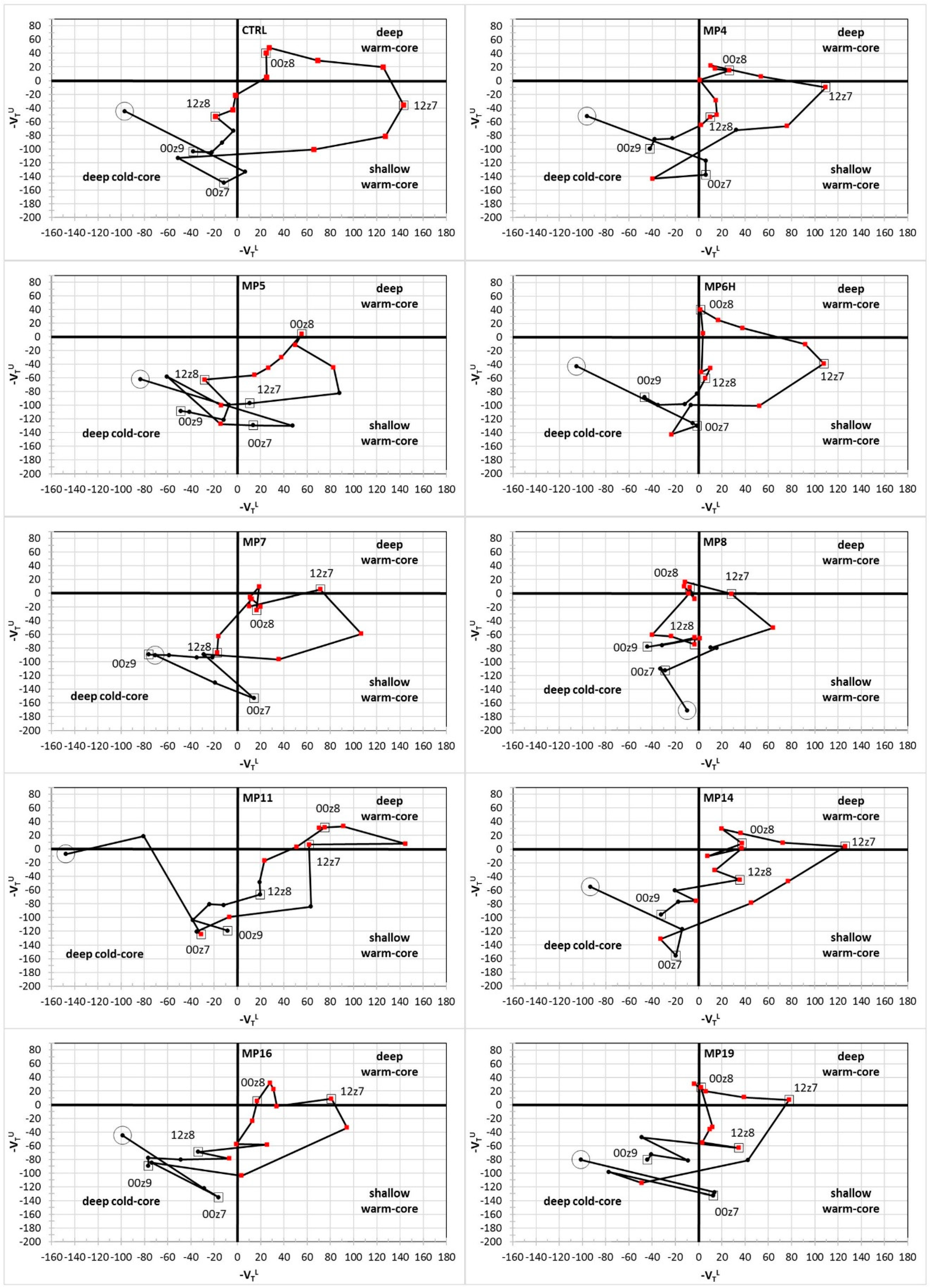
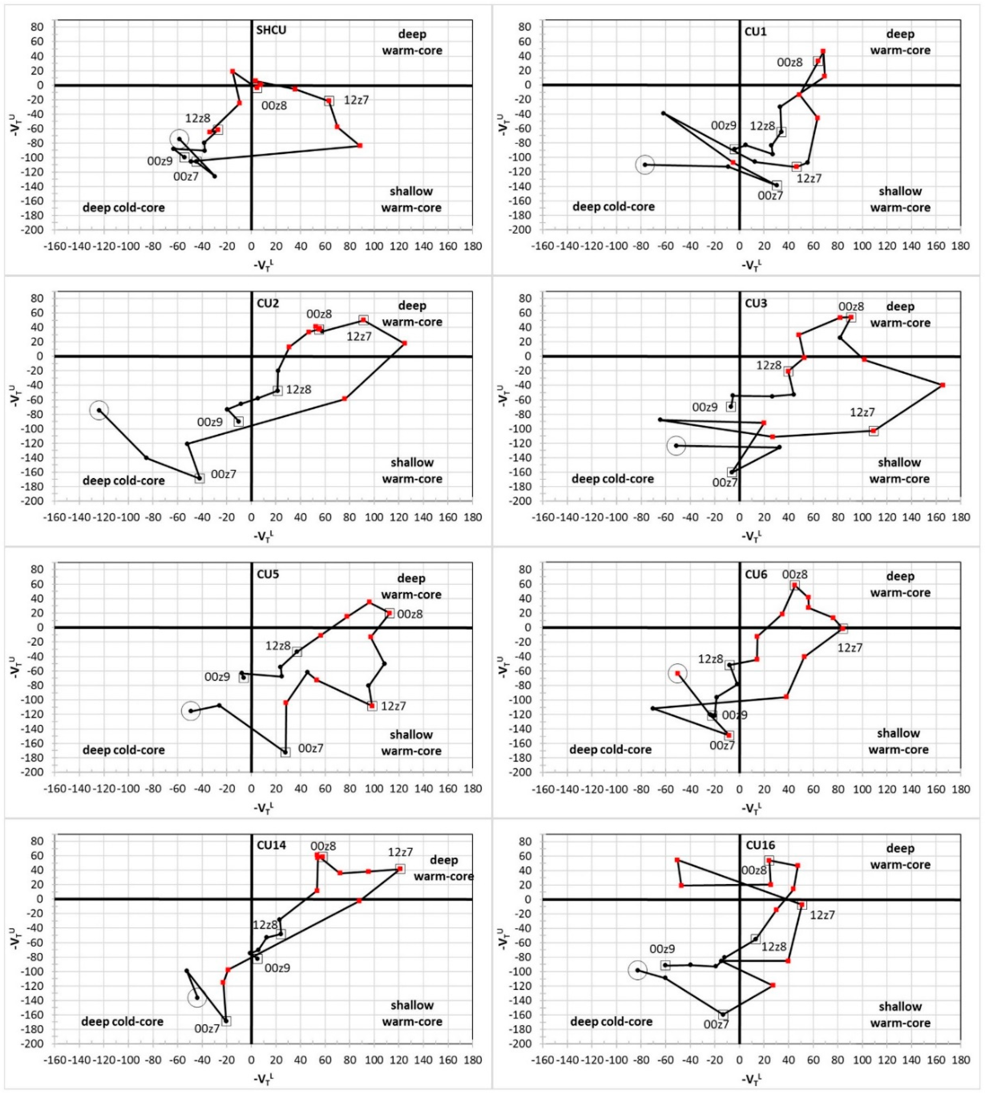
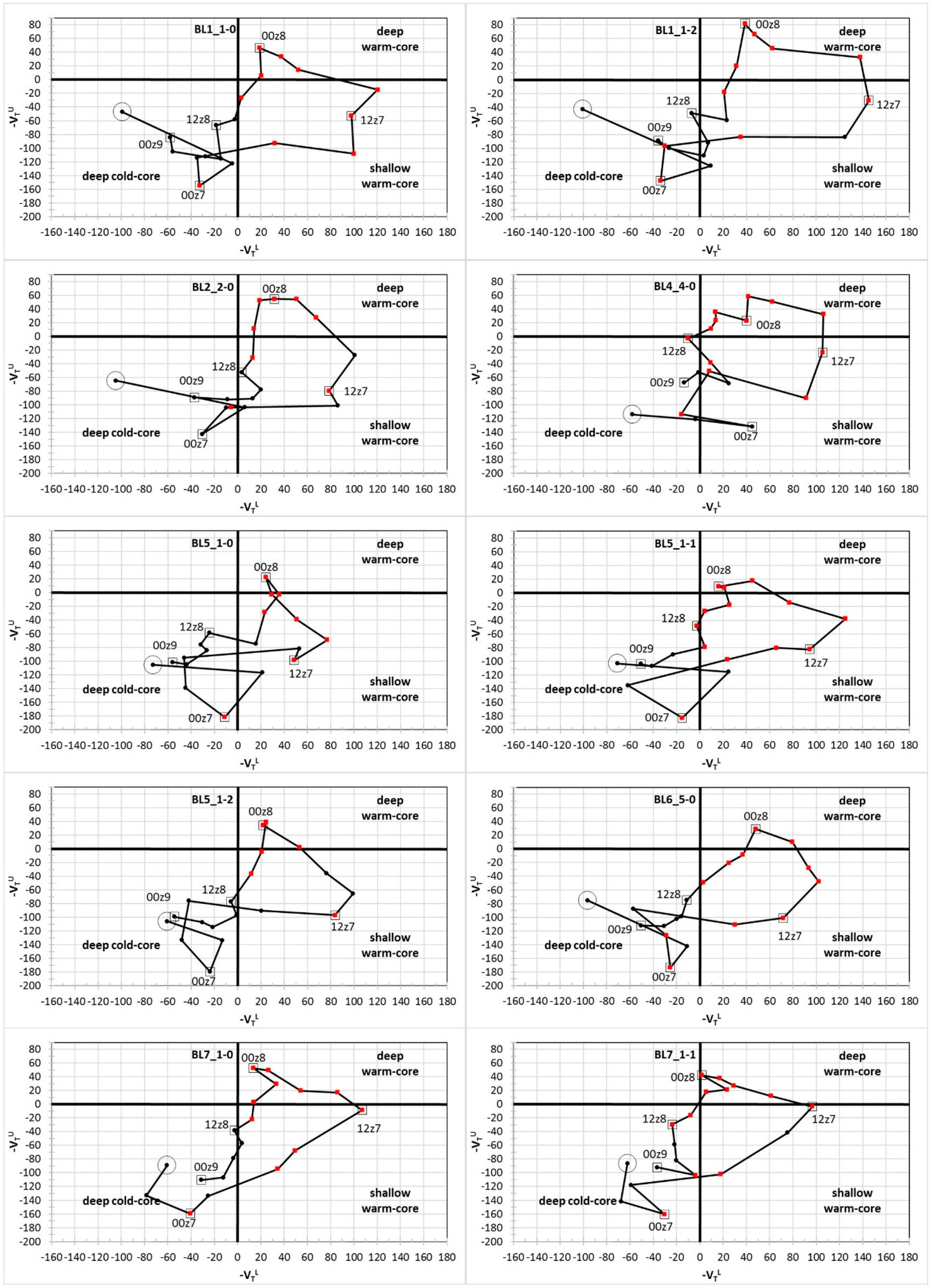
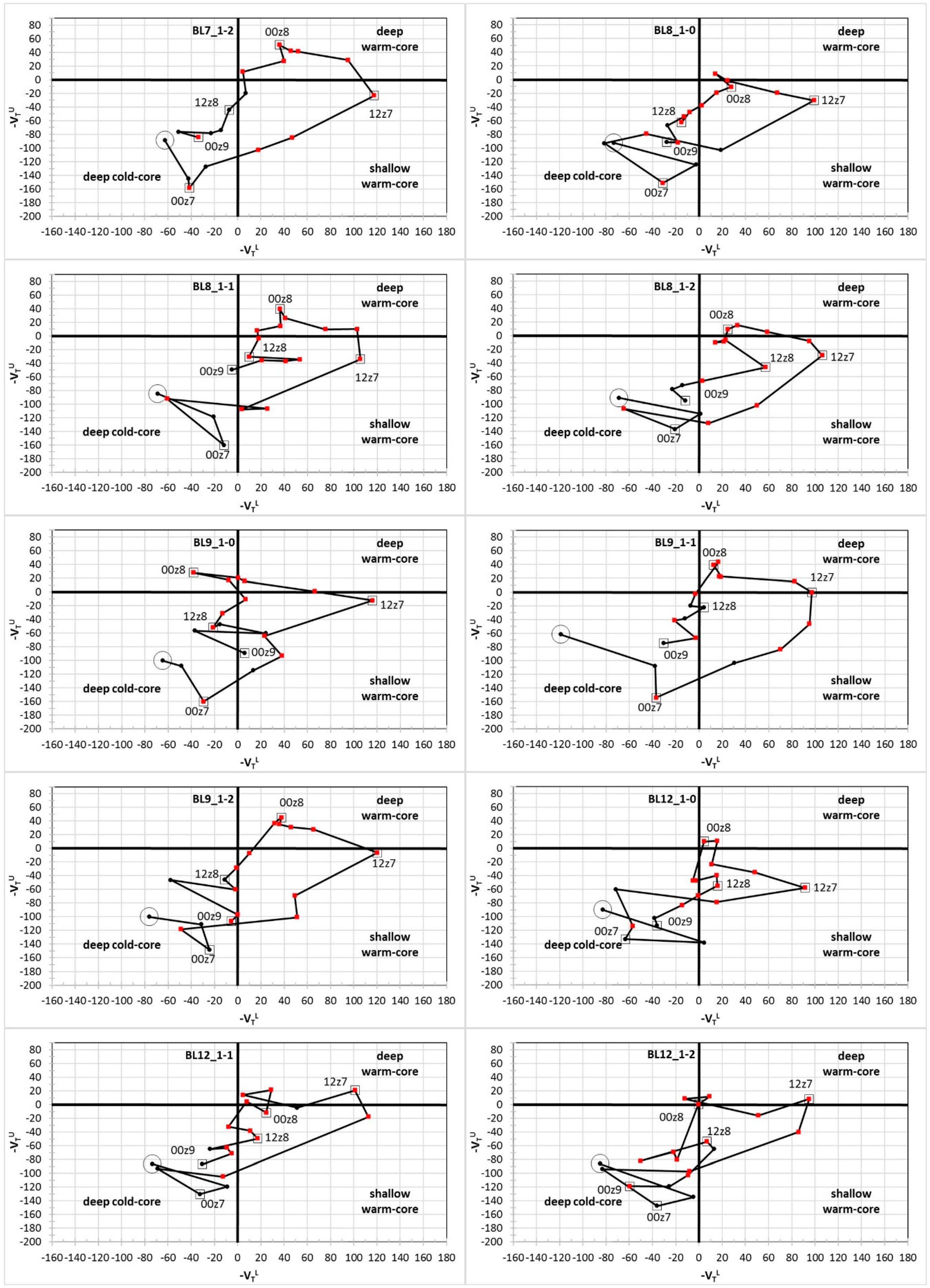
2.2. Phase Space Diagrams

The phase space diagrams are utilized in order to objectively determine the thermal structure of the cyclone and the occurrence of a medicane [69]. The thermal symmetry/asymmetry parameter B is calculated in the layer 900–600 hPa, and it represents the difference of the layer mean thickness of the right side minus that of the left side of the cyclone. The two sides of the system are defined relative to its direction of movement. Values of B smaller than 10 m indicate thermally symmetric systems, similar to the tropical cyclones [69,70]. The warm/cold core vertical structure of the cyclone is determined through the scaled thermal wind magnitude at a lower ($-{\mathrm{V}}_{\mathrm{T}}^{\mathrm{L}}$; 900–600 hPa) and an upper ($-{\mathrm{V}}_{\mathrm{T}}^{\mathrm{U}}$; 600–300 hPa) tropospheric layer, which is in line with Pytharoulis [8], Miglietta et al. [18,31], Chaboureau et al. [19], Hart [69]. A linear regression fit, with a vertical increment of 50 hPa, is used to calculate the two thermal wind parameters. Positive (negative) values of $-{\mathrm{V}}_{\mathrm{T}}^{\mathrm{L}}$ and $-{\mathrm{V}}_{\mathrm{T}}^{\mathrm{U}}$ denote the occurrence of a warm (cold) core at each layer. B, $-{\mathrm{V}}_{\mathrm{T}}^{\mathrm{L}}$, and $-{\mathrm{V}}_{\mathrm{T}}^{\mathrm{U}}$ are calculated within a radius of 200 km around the minimum mslp of the low, following Pytharoulis [8], Chaboureau et al. [19], and Miglietta et al. [31] who have employed this radius successfully in the study of TLC14 and the medicane of September 2006 in southern Italy, respectively (while they had performed sensitivity tests for other radii). Using the above criteria, a medicane, which is a thermally symmetric cyclone with a deep warm core, is considered to occur when simultaneously B < 10 m and $-{\mathrm{V}}_{\mathrm{T}}^{\mathrm{L}}$, $-{\mathrm{V}}_{\mathrm{T}}^{\mathrm{U}}$ are both positive.

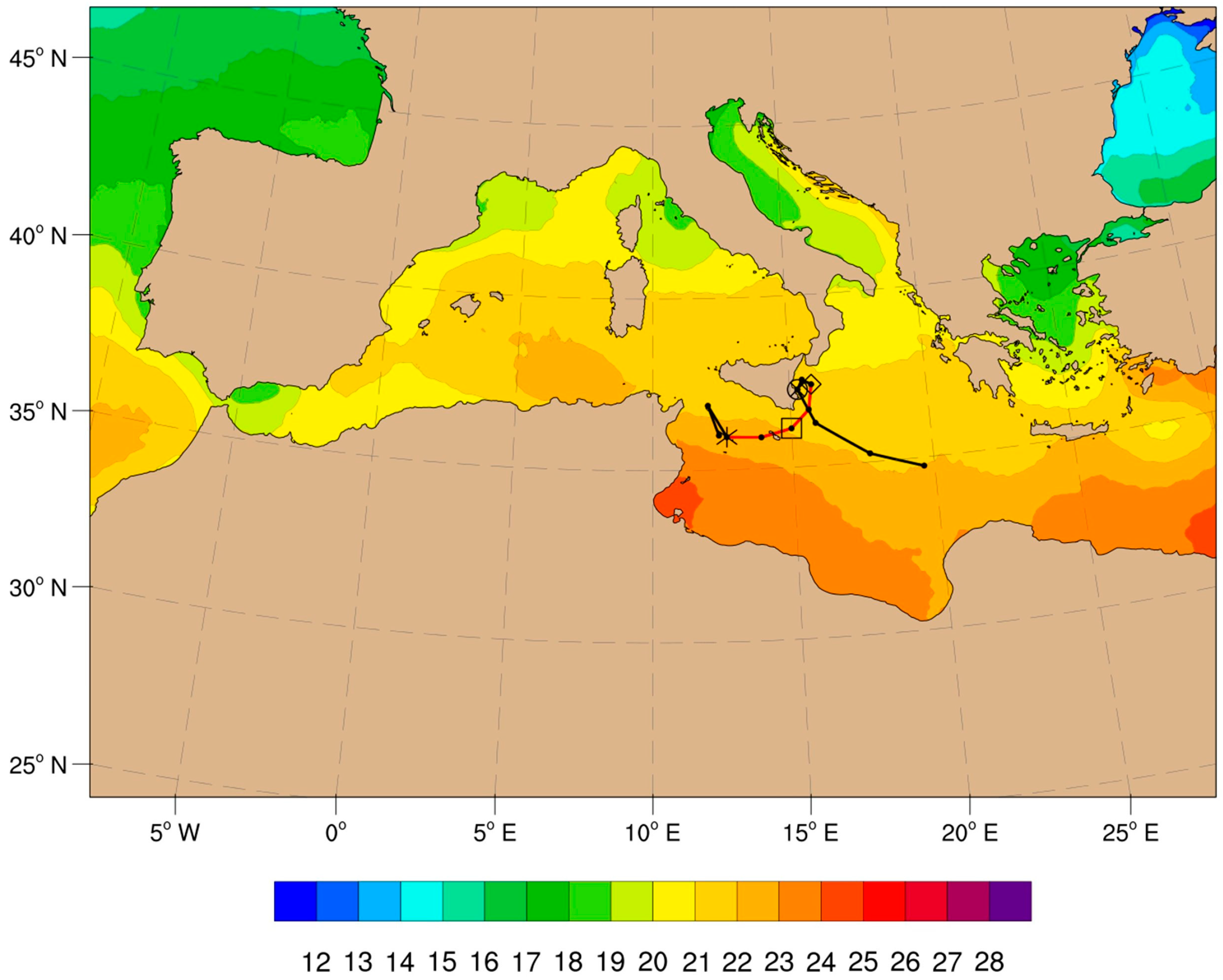
2.3. Synoptic Overview

TLC14 formed south of Sicily on 7 November 2014, because of the interaction of a pre-existing baric low associated with a low-level baroclinic zone with a tropopause anomaly. The depression emerged from Libya at 12:00 UTC on 6 November 2014. Carrio et al. [23] pointed out the role of the upper air PV anomaly for the development of TLC14, via numerical experiments with a modified upper air PV field. Scale contraction and rapid deepening of 8.3 hPa occurred from 00:00 to 06:00 UTC on 7 November 2014. A sub-synoptic scale cyclonic circulation, with a hook at its center [35], appeared in the satellite imagery between Lampedusa and Pantelleria islands at about 08:00–9:00 UTC on 7 November 2014 [8]; in the following few hours (10:00–12:00 UTC) the medicane, with a clear cloud-free ‘eye’ and a spiral bands of clouds, formed. A maximum 10-min sustained wind speed of 23.7 m/s was recorded at Lampedusa at 12:06 UTC, while the gusts reached 37.6 m/s. TLC14 made landfall in Malta, and a record minimum mslp of 984 hPa (SPECI report) was reported by its airport (LMML) at 16:34 UTC on 7 November 2014. Then, the system headed north–northeastward (Figure 1), and its ‘eye’ made landfall in eastern Sicily in the early hours of 8 November (~04:30 UTC), without moving farther over land. Significant damages were caused in the greater area of Catania [8]. The “best” track of Figure 1 has been adopted from Pytharoulis [8]. It was based on the location of the medicane’s ‘eye’ in the three-hour Meteosat satellite images (10.8 μm), from 12:00 UTC 7 November to 06:00 UTC 8 November 2014, when it exhibited tropical features in the satellite imagery. The tracks of the parent low and the cyclone that remained after the medicane lost its tropical characteristics are based on the minimum mslp of the depression in the six-hour ECMWF operational analyses. The phase space diagrams [69] of the six-hour ECMWF analyses (0.125° × 0.125° latitude–longitude), produced for the layers 900–600 hPa and 600–300 hPa within a radius of 200 km around the mslp center of the cyclone, showed that it exhibited a symmetric deep warm-core structure from 12:00 UTC 7 November to 00:00 UTC 8 November (presented in Figure 5 of Pytharoulis [8]). A symmetric shallow warm-core was present at 06:00 UTC 8 November. In the following hours, the cyclone headed southeastward (Figure 1), started to lose its tropical features in the satellite images, decayed, and became an asymmetric deep cold-core cyclone. Further detailed analysis of the observed system has been provided by Pytharoulis [8], Carrio et al. [23], and Dimitriadou [35].

3. Results and Discussion

The results of the numerical experiments, regarding the sensitivity of the simulated TLC14 to the microphysical, cumulus, and boundary layer/surface layer parameterizations, are presented and discussed in this section. The analysis is mainly based on the cyclone’s track, intensity (measured by its minimum mean sea-level pressure), thermal symmetry, and vertical thermal structure.

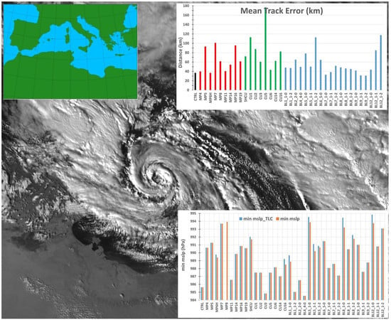
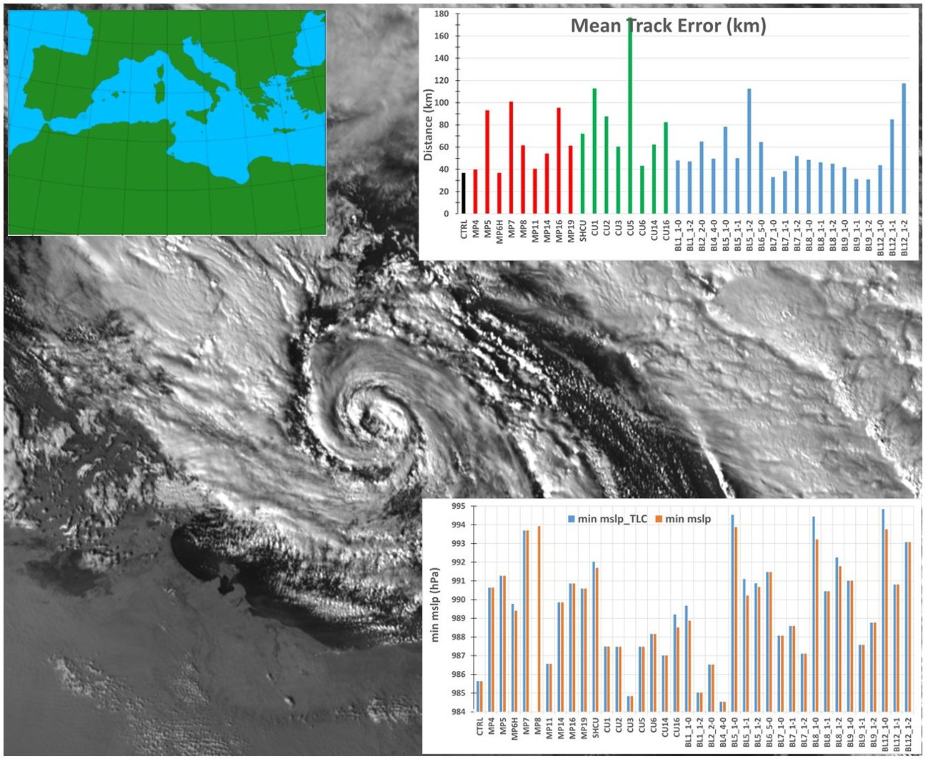
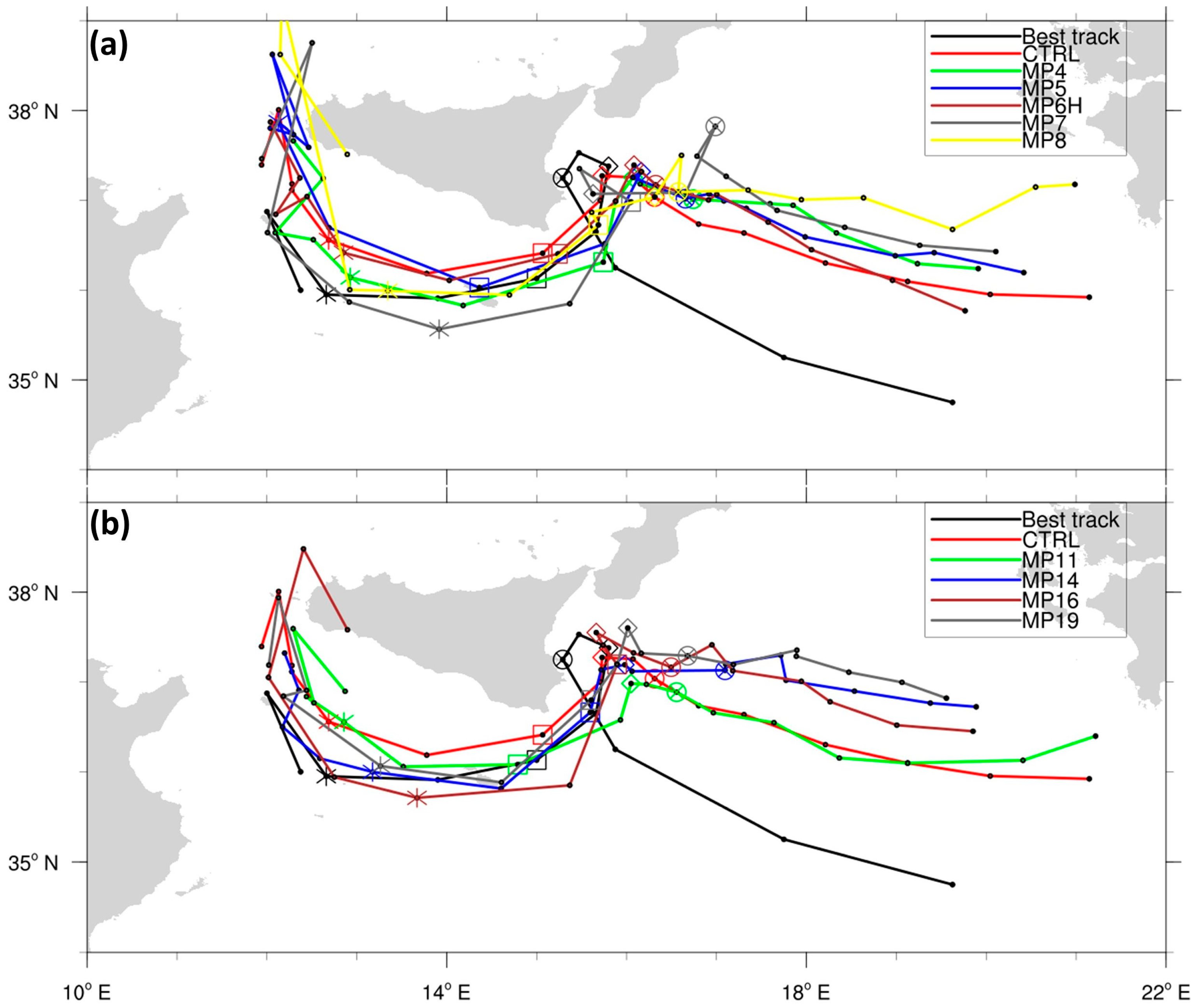
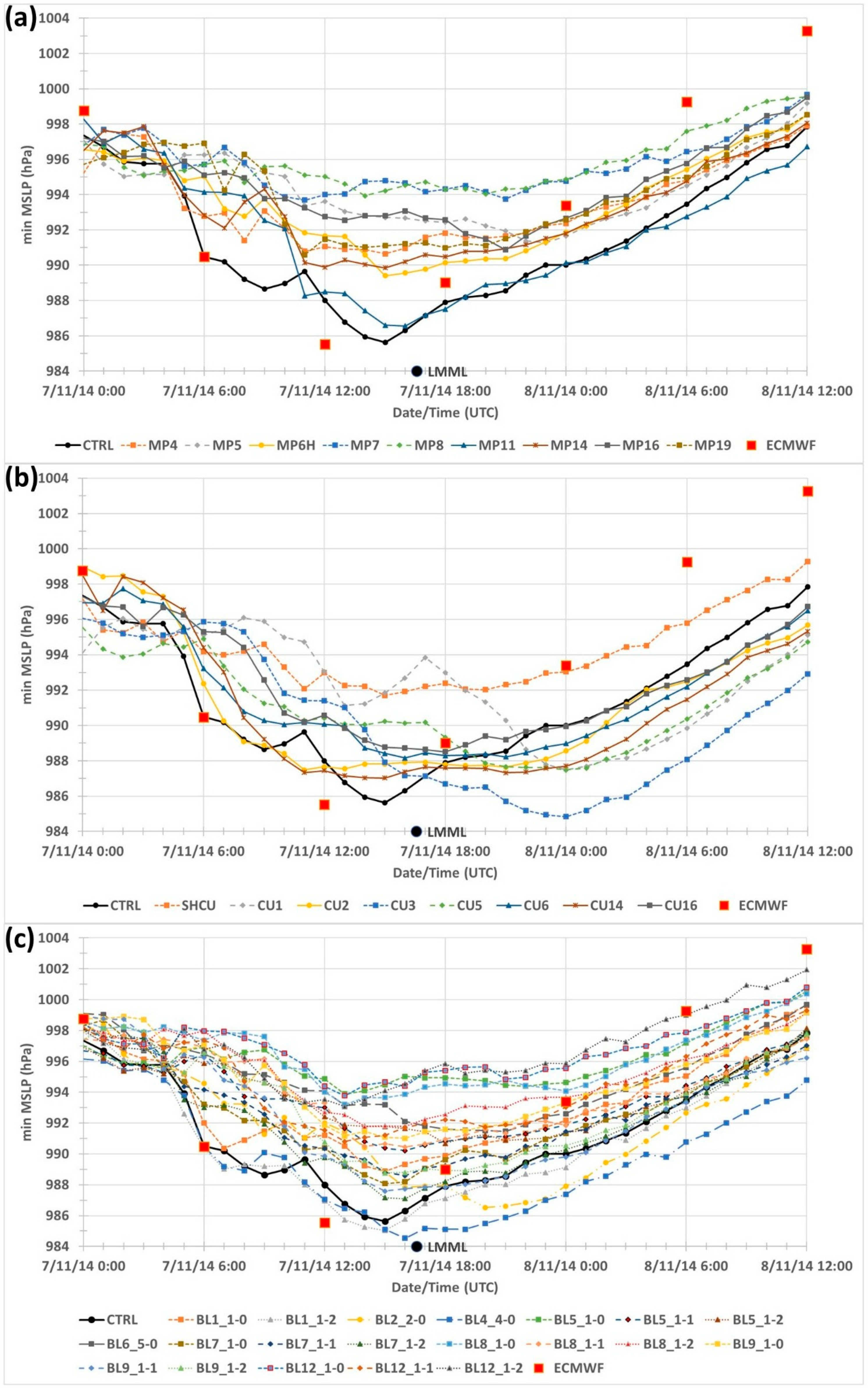
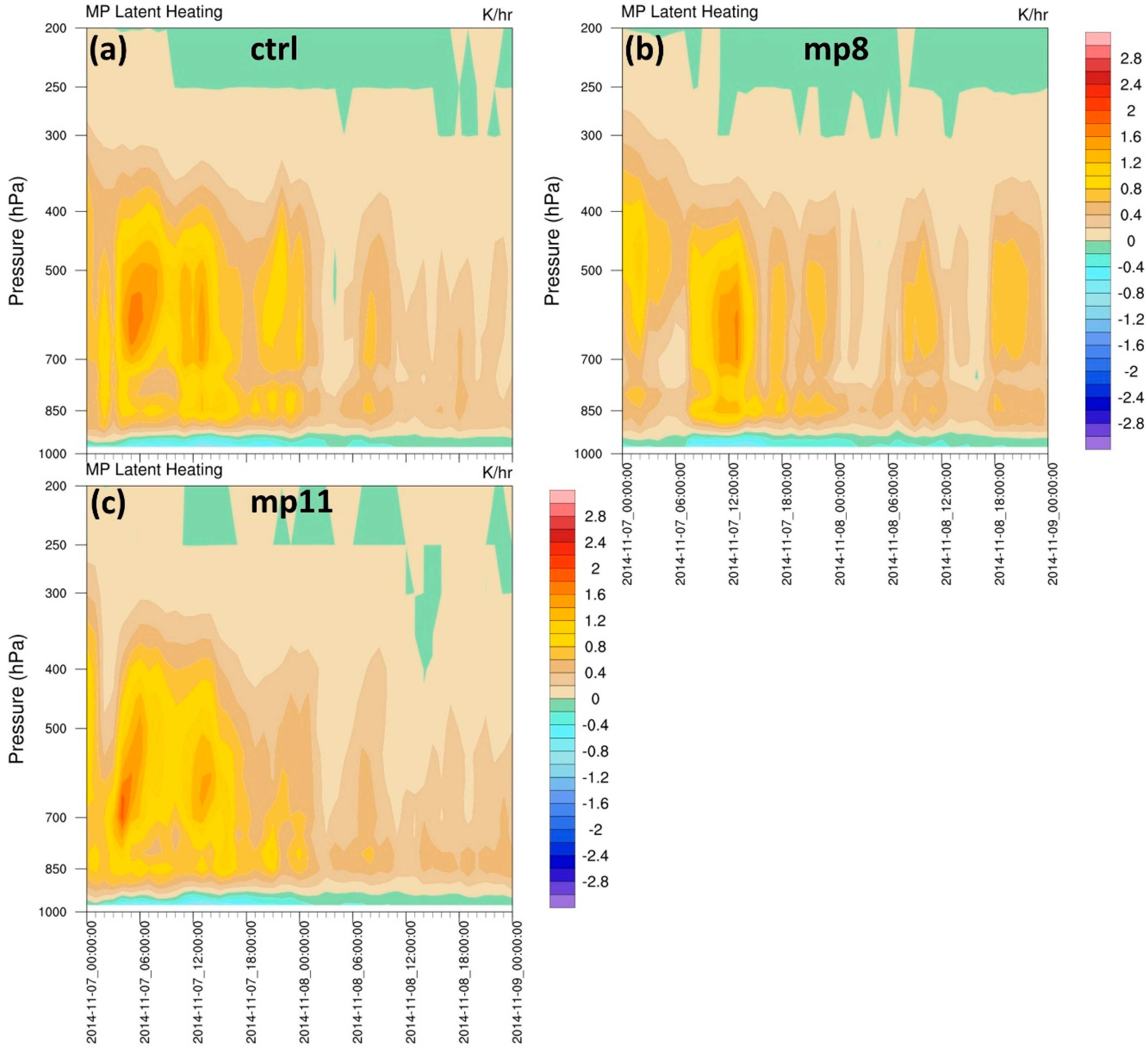
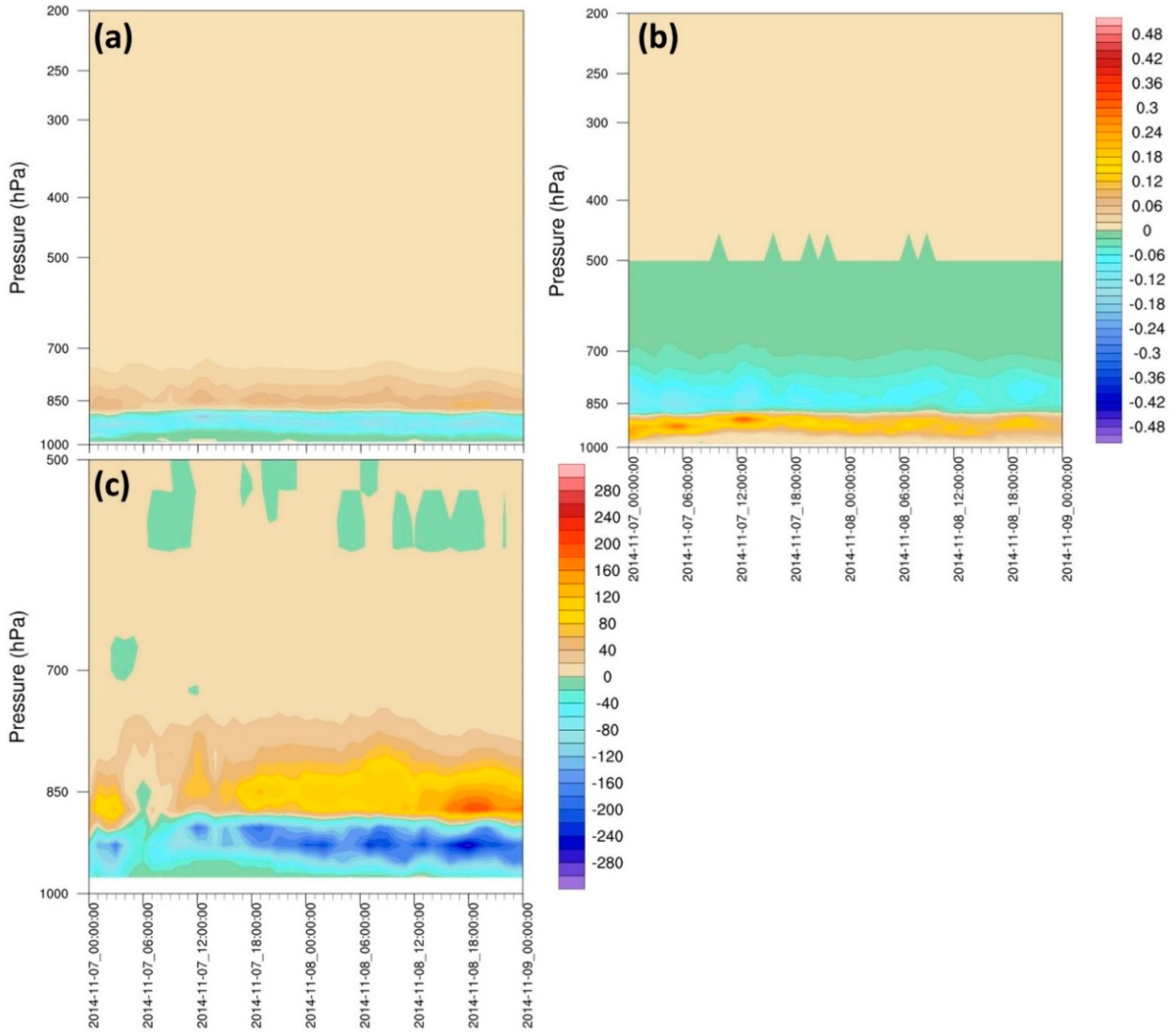
3.1. Microphysical Parameterizations

Microphysical parameterizations with different complexities and species, and some of them including graupel, hail, or both (Table 1), were implemented in the numerical experiments. The experiment mp6h is identical to ctrl, but it replaces the graupel with hail.

Figure 2 illustrates the tracks of the simulated parent low, the medicane, and the cyclone that remained after it lost its tropical features in the experiments with different microphysics (including ctrl), together with the “best” track of the observed TLC14 and the lows before and after its occurrence. The minimum mslp of the low was followed in order to derive the track in each experiment. The tracks generally followed the path of the actual TLC14 from 12:00 UTC 7 November to 00:00 UTC 8 November, when the cyclone exhibited a symmetric deep warm core in the ECMWF analyses, with most of the simulated tracks misplaced to the northern side. In mp4, mp8, mp14, and mp19, they passed over Malta. However, no experiment managed to simulate the landfall at eastern Sicily or follow closely the track of TLC14 after it lost its tropical characteristics (although they moved in the correct southeastward direction).

The mean distance of the three-hour locations of the simulated tracks from the “best” track, which were averaged from 12:00 UTC 7 November 2014 to 00:00 UTC 8 November 2014, is displayed in Figure 3. Regarding the mp experiments, the smallest track errors (36.9 km) were associated with the ctrl and mp6h experiments. These simulations were successful, considering that the mean distance of the minimum mslp in the six-hour ECMWF analyses from the “best track” at the same period was about 20 km. The cyclone followed very close paths in ctrl and mp6h, with the latter cyclone being slightly to the east of the former one at all of the three-hour intervals of this period. Therefore, the use of graupel (ctrl) or hail (mp6h) in the WSM6 scheme did not appear to affect the mean distance of the simulated cyclone from the actual one. The next successful experiments in terms of track were mp4 and mp11, which produced mean errors of 39.8 km and 40.5 km, respectively (Figure 3). Both WSM5 (in mp4) and CAM5.1 (in mp11) parameterizations are five-class without graupel or hail. In agreement with Miglietta et al. [31], it seems that relatively simpler schemes such as WSM5 may reproduce the track of the medicane adequately. The mp experiments with the largest track errors were mp5 (93.3 km), mp16 (95.5 km), and mp7 (100.9 km). Similarly to Miglietta et al. [31], the double-moment six-class WDM6 (mp16) scheme with graupel was much less successful than the simpler single-moment five-class WSM5 (mp4) and the double-moment five-class WDM5 (mp14) schemes, which did not include graupel (Figure 3).

The time series of the minimum mslp of TLC14 and its parent low (Figure 4a) showed a significant sensitivity of the intensity to the choice of the microphysical scheme. Ctrl (with WSM6) and mp11 (with CAM5.1) were the only mp experiments that simulated the rapid deepening of the cyclone properly, reaching a minimum mslp of 985.6 hPa and 986.6 hPa, at about 1.5 h and 0.5 h (respectively) prior to the minimum mslp measurement of 984 hPa at Malta (LMML). Mp6h simulated the next deeper cyclone with a minimum mslp of 989.4 hPa at the same time as ctrl. It seems that the use of graupel in ctrl, instead of hail in mp6h, resulted in a deeper cyclone by 3.8 hPa in the former experiment, as both experiments employed the WSM6 scheme and followed very close tracks (Figure 2) over similar SSTs. The average (maximum) SST difference, in a radius of 200 km around the minimum mslp, was equal to 0.02 °C (0.26 °C). This result agrees with Wang [71] (as shown in his Figure 2b), who simulated a tropical cyclone with a triple nested model (45 km, 15 km, 5 km) without a cumulus scheme, and produced a slightly deeper cyclone (by a few hPa) when graupel was employed instead of hail. The weakest development was exhibited by mp7 and mp8, in which the lowest pressure reached 993.7 hPa and 993.9 hPa, respectively (Figure 4).

The phase space diagrams allowed the analysis of the structural evolution of TLC14 in the various experiments and the objective determination of the occurrence of a symmetric deep warm-core cyclone (TLC). In Figure 5, the existence of a medicane is indicated by the occurrence of a symmetric cyclone (B < 10 m; red squares) at the same times with a deep warm core (at both layers 900–600 hPa and 600–300 hPa). These diagrams have been calculated at three-hour intervals. Figure 5 shows that ctrl and mp11 predicted a TLC in the periods 15:00 UTC 7 November to 03:00 UTC 8 November, 12:00 UTC 7 November to 03:00 UTC 8 November, which was for a longer duration than most of the other mp experiments, and particularly mp7 and mp8 (with the weakest development). The thermal symmetry and the warm-core criteria were not met simultaneously at any three-hour timestep in mp8, and a TLC did not form. Moreover, the warm core of both layers was less pronounced in mp7 and mp8 than in ctrl and mp11. In mp6h, the use of hail resulted in the occurrence of a weaker warm core. Although the two experiments with the WRF single-moment and double-moment five-species schemes (mp4 and mp14) attained a symmetric deep warm core for the same duration as ctrl (15 h) and mp11 (18 h), respectively, they exhibited a weaker development (in terms of mslp; Figure 4a), which was probably due to the existence of a weaker warm core (Figure 5). Therefore, it appears that the microphysical parameterization affects the structure of the simulated cyclone, as well as the duration and strength of a symmetric deep warm core, and in turn it influences the intensity of the system (in terms of the minimum mslp).

Figure 6 shows that stronger latent heating was provided to the cyclone in the experiments where the lowest mslp was reached (ctrl and mp11) rather than in mp8, which did not attain a symmetric deep warm-core low. For example, values higher than 0.8 K/hr appeared for a longer period before the formation of the medicane in the former two experiments, and they extended at higher levels (marginally above 400 hPa), assisting the formation of the upper-level warm core directly, as well as indirectly through the secondary circulation. The maximum latent heating was simulated at about 700–500 hPa, while Wang [71] estimated it in the mid–upper troposphere (5–8 km) in the eyewall of tropical cyclones. The occurrence of convective bursts, with latent heating maxima up to about 1.6–2.0 K/h, before the formation of the medicane was also reported by Pytharoulis [72], in a simulation relative to the transformation of a cold-core African easterly wave into hurricane Felix (of 1995) in the tropical north Atlantic. Their role was to induce the contraction of the horizontal scale of the incipient low and the increase of the low-level vorticity, assisting the WISHE (wind-induced surface heat exchange) mechanism [73]. In turn, the Rossby radius of deformation was reduced, keeping the temperature anomalies, due to convection, more localized [74]. The Rossby radius of deformation (λ) is calculated by λ = ΝH/(f + ζ), where N is the Brunt–Vaisala frequency, H is the depth scale, f is the coriolis parameter, and ζ is the vertical component of the relative vorticity.

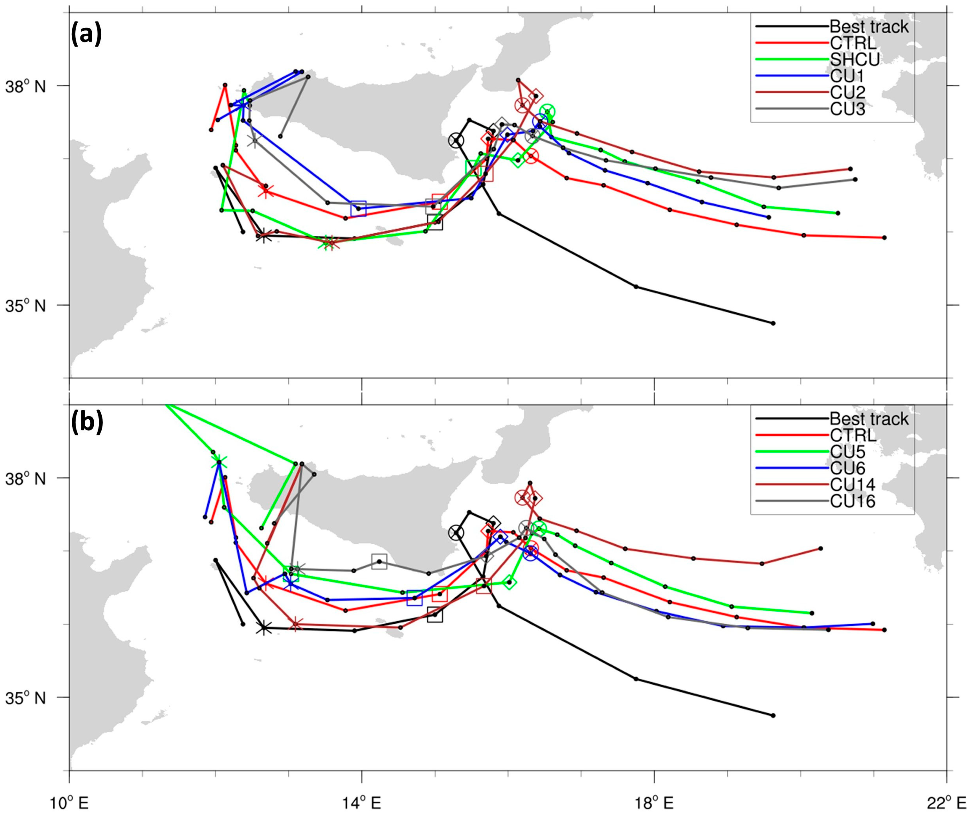
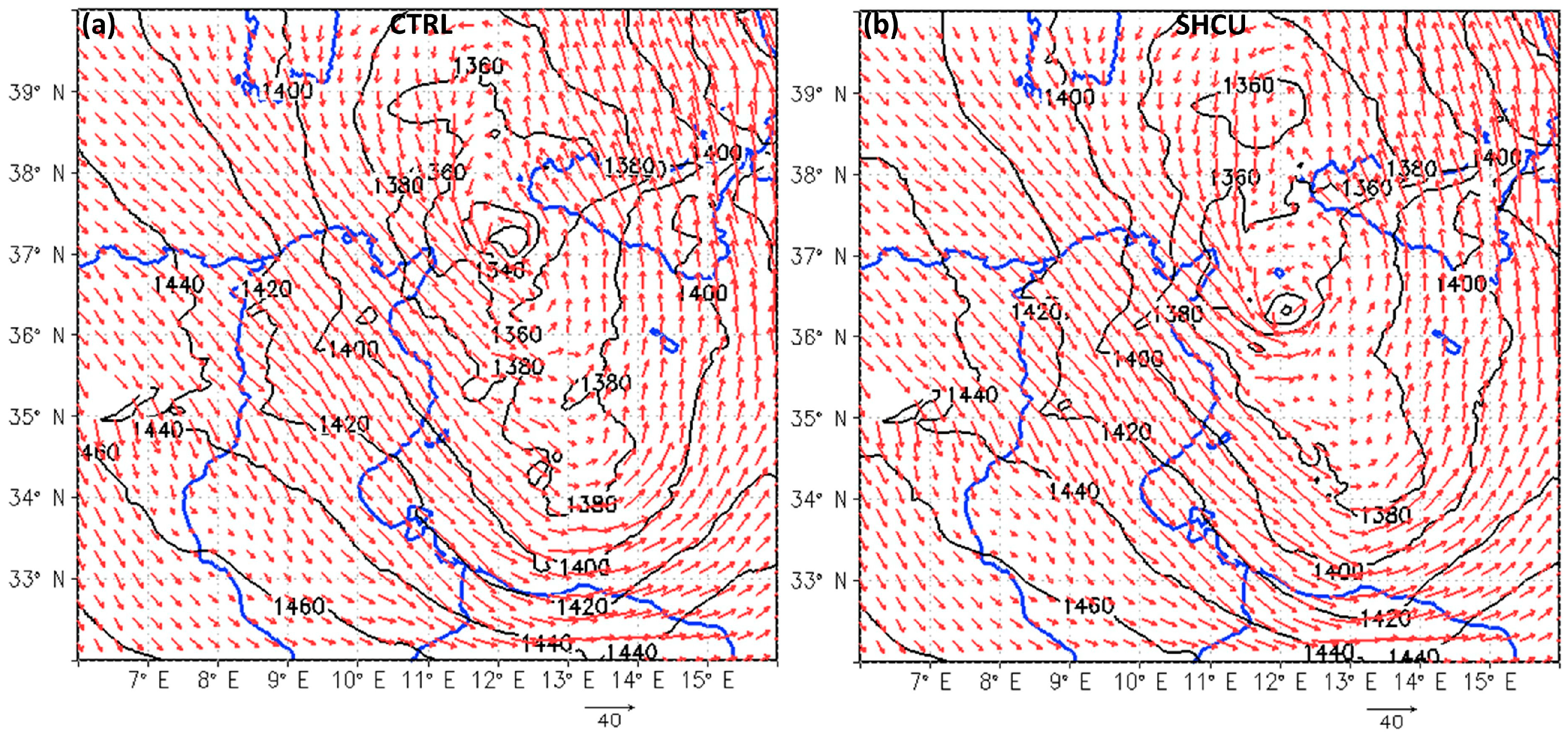
3.2. Cumulus Parameterizations

The influence of the representation of cumulus convection in the WRF simulations of TLC14 is investigated here. The control experiment reproduced convection explicitly. Shallow cumulus clouds have typical sizes of about 1 km [75], and cannot be resolved by the grid-spacing of the current model setup (7.5 km). For this reason, the shcu experiment was considered: it was identical to ctrl, but it parameterized shallow convection through the GRIMS scheme (Table 1), in order to examine its effect on the simulated medicane. The other experiments of this subsection defined the cumulus schemes using different formulations, namely mass flux (cu1, cu6, cu14, cu16), convective adjustment (cu2), and ensemble mean (cu3, cu5) approaches.

Figure 7 shows that in most of the cu experiments, the cyclone moved on the northern side of the observed TLC14’s path or over it (shcu, cu2, cu14) until it reached the Ionian Sea east of Sicily (at about 18:00 UTC 7 November to 00:00 UTC 8 November), which was in satisfactory agreement with the observations. As a result, in these three experiments, the cyclone made landfall on the island of Malta. In contrast to the actual system, the depression in cu16 crossed southeastern Sicily. No experiment managed to reproduce the landfall at eastern Sicily. The distance of the three-hour locations of the simulated cyclone from the “best” track, averaged from 12:00 UTC 7 November to 00:00 UTC 8 November, was minimized by ctrl (36.9 km) and cu6 (43.3 km), and was maximized by cu1 (112.8 km) and cu5 (176.7 km) (Figure 3). Torn and Davis [76] concluded that their hurricane WRF forecasts, which were initialized by a data assimilation system that employed the Tiedtke scheme, produced 25% smaller track errors than using the Kain–Fritsch scheme. The three experiments that simulated the cyclone approximately on the same path as the actual system until its western turn east of Sicily produced much larger errors of 62.2 km (cu14), 72.1 km (shcu), and 87.6 km (cu2). The use of the new SAS, GRIMS (for shallow convection), and BMJ schemes improved the path of the cyclone (relative to ctrl), although the distance from the actual system deteriorated because of a different translation speed. These results partly agree with Han and Pan [54], Torn and Davis [76], and O’Shay and Krishnamurti [77], who have shown that the inclusion of shallow convection in the numerical models improved the predicted track of the tropical cyclones. The examination of the low-level wind flow in ctrl and shcu at 06:00 UTC 7 November (Figure 8) suggests that the improved trajectory of the latter simulation south of Sicily was due to the more southern location of the parent low relative to the ctrl at that time. This allowed the northwesterly flow at the west of the trough to move the parent low of shcu along the correct path, but at a faster speed than the ctrl, during this period. Therefore, the track error seems to be influenced by the relative position of the medicane and its parent low with respect to the ambient steering flow.

The maximum deepening of the cyclone was attained by cu3 and ctrl, which reached 984.8 hPa and 985.6 hPa, respectively (Figure 4b). However, the intensification in cu3 commenced about four hours after ctrl, and the lowest mslp was simulated at 00:00 UTC 8 November over the Ionian Sea east of Sicily, instead of the region of Malta. The weakest development was exhibited in shcu, in which the mslp dropped to 991.7 hPa. Zhu and Smith [78] concluded that shallow convection reduces the intensification rate of tropical cyclones, because it transports low moist static energy air from the lower troposphere to the boundary layer, inhibiting convection. In the other cu experiments, the minimum mslp of the cyclone ranged only from 987.0 to 988.5 hPa, but the time of maximum intensity (in terms of mslp) varied from 11:00 UTC 7 November (in cu2) to 00:00 UTC on 8 November (in cu1, cu5).

Figure 9 shows that there was a large variability in the duration of the medicane, which ranged from 21 h in cu2 and cu14 to six hours (only) in shcu. In all of the cu experiments (except from cu16), a lower layer (900–600 hPa) symmetric shallow warm core preceded the formation of the medicane. The experiment with the lowest mslp (cu3) exhibited the strongest low-level thermal wind magnitude (maximum $-{\mathrm{V}}_{\mathrm{T}}^{\mathrm{L}}$; before its TLC phase) and a pronounced upper layer (600–300 hPa) warm core. On the contrary, shcu (with the weakest intensity in terms of mslp) formed a marginal warm core in the upper layer. Pytharoulis [8] showed that the WRF experiments of TLC14 with a less pronounced upper layer warm core resulted in a weaker medicane.

The heating rates from the microphysics and the deep convection schemes are presented in Figure 10 for the experiments with the strongest and the weakest intensity (regarding mslp). In cu3 (Figure 10a), heating up to 1.4–1.6 K/h (averaged in radius of 200 km) was provided to the parent low by the microphysics scheme prior to the formation of the medicane. However, the strongest heating in this cyclone was triggered later than in ctrl (Figure 6a), which was consistent with its delayed development in terms of mslp (Figure 4b) and medicane formation (Figure 5 and Figure 9). After about 15:00 UTC 7 November, the cumulus scheme dominated in warming the mid–low levels of the cyclone (with rates up to 0.8–1 K/h; Figure 10c). On the other hand, the grid-scale microphysical parameterization reduced the low-level net heating, with minima of −0.2 to −0.4 K/h at around 700 hPa, which was probably due to rain evaporation and/or snow and graupel melting, since the freezing level was located at about or just above 700 hPa in a radius of 200 km around the medicane and its parent low (not shown).

The comparison of ctrl (Figure 6a) with shcu (Figure 10b), which attained a much shorter duration of the symmetric deep warm core and a weaker cyclone (by 6.1 hPa) than ctrl, reveals that the microphysics heating rates of the parent low in the latter run were stronger than in the control one. The representation of shallow convection (in shcu) improved the path of the parent low before TLC14 formation (Figure 7a), and the depression moved over warmer SSTs (up to 0.7 °C in a radius of 200 km) than ctrl. This may explain the higher heating rates of shcu, which might have been due to the stronger sea surface sensible and latent heat fluxes in this phase. However, the system in shcu reached the colder SSTs located east of Sicily (Figure 1) earlier than in the ctrl and in the observed one (Figure 7a). As a result, the medicane of shcu formed over colder SSTs, and the sea surface latent and sensible heat fluxes (averaged in a radius of 200 km around the min mslp) were lower than in the ctrl (reaching a difference of −112.6 W/m² at 18:00 UTC 7 November 2014). Moreover, Figure 11a,b shows that the shallow convection acted to dry and warm the boundary layer of the simulated cyclone, while it moistened and cooled the lower troposphere above it, as in reality. The combination of these temperature and moisture tendencies resulted in the reduction of the moist static energy in the boundary layer of the storm (Figure 11c), stabilizing the parent low and the medicane to convection. This mechanism explains the delayed formation (by three hours) and the shorter lifetime (by nine hours) of the medicane in shcu, relative to ctrl. It is also in agreement with Zhu and Smith [78], who concluded that shallow convection stabilizes the tropical cyclones to convection through the transport of low moist static energy air from the lower troposphere to the boundary layer. However, they used an idealized tropical cyclone model with constant SSTs at 28 °C [79], while in the present study, there was spatial variability of SSTs, which locally modified the boundary layer thermodynamic state together with the shallow convection.

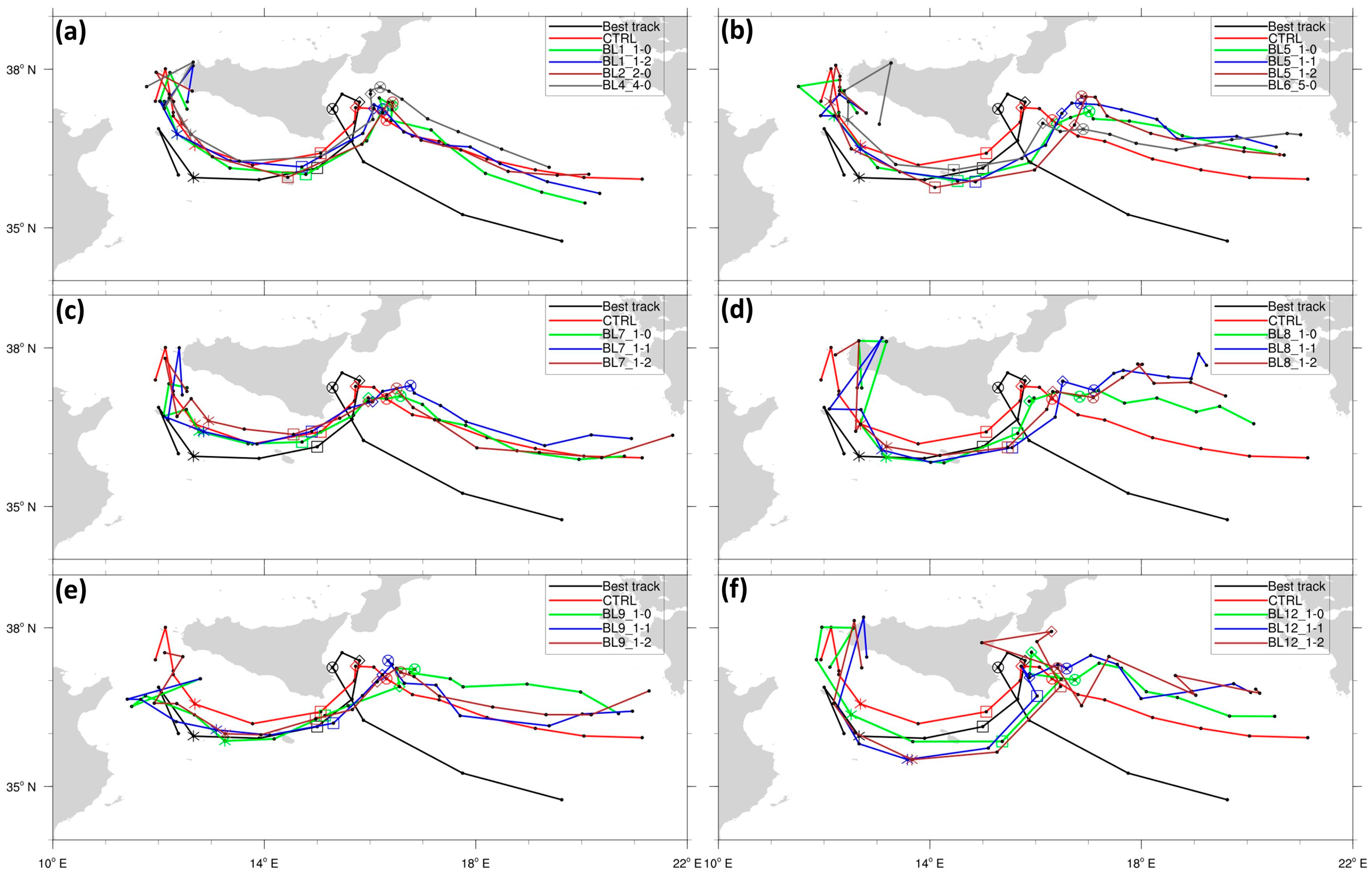
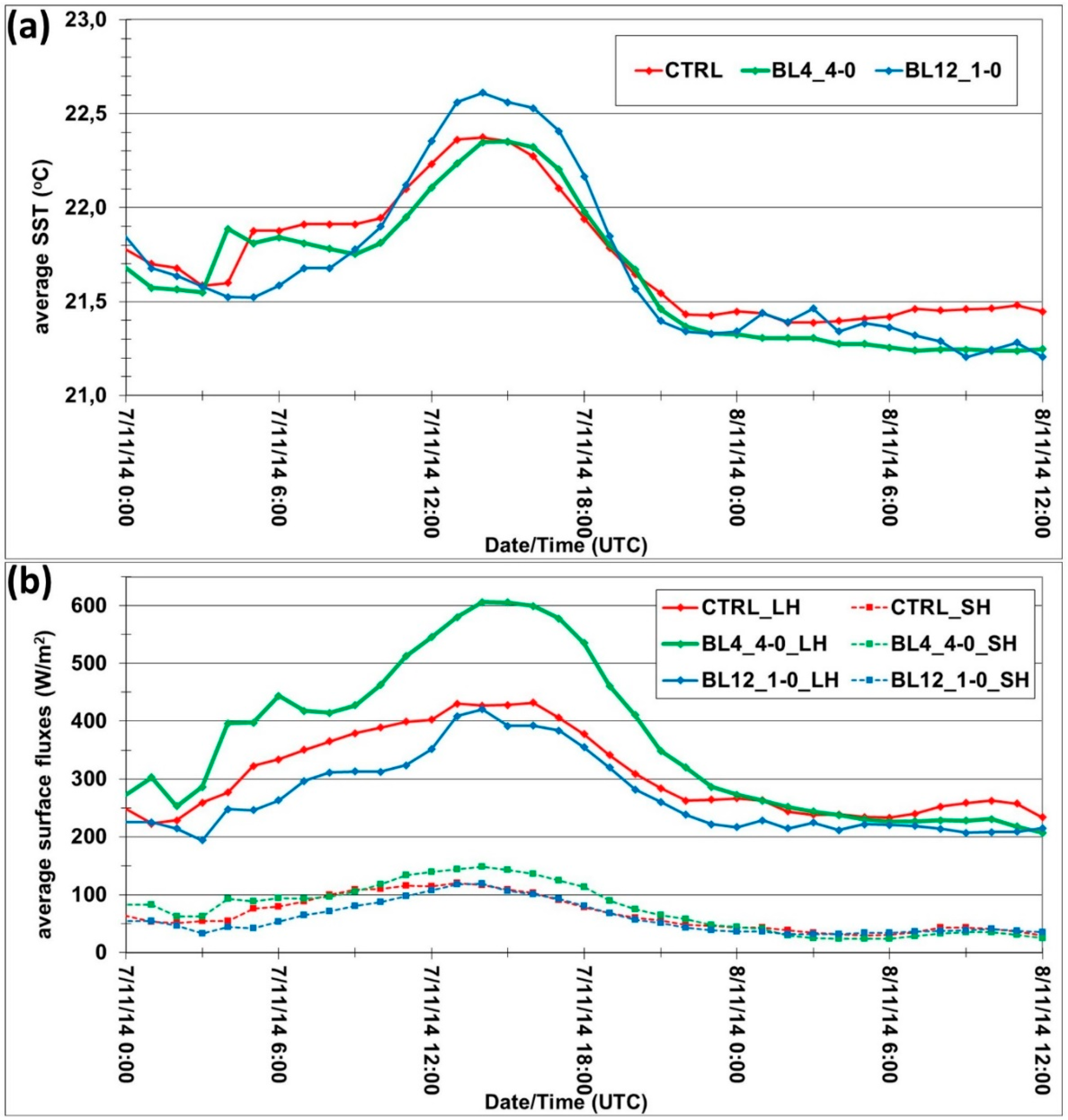
3.3. Boundary Layer/Surface Layer Parameterizations

The medicane and its parent low in the experiments with the different boundary/surface layer parameterizations (bl) exhibited a variability in the path (Figure 12), passing on either sides of the actual track until the simulated cyclones reached the Ionian Sea east of Sicily, while afterwards, it moved north of the observed cyclone toward Greece in all of the simulations. Several experiments represented the landfall at Malta, but only bl12_1-2 (Figure 12f) predicted the landfall in eastern Sicily at 03:00 UTC on 8 November 2014, which was in good agreement with observations. Despite this achievement, bl12_1-2 had the largest track error of 117.4 km in the previous period (12:00 UTC 7 November to 00:00 UTC 8 November 2014) (Figure 3). The smallest track errors in this period were associated with the boundary layer schemes UW (bl9_1-2 = 30.9 km, bl9_1-1 = 31.4 km) and ACM2 (bl7_1-0 = 32.9 km, bl7_1-1 = 38.5 km), while the control run (equivalent to bl1_1-1), which employed the YSU scheme, had the fourth lowest error of 36.9 km (Figure 3).

The different boundary and surface layer parameterizations (with or without modifications in the formulation of the surface fluxes) resulted in a wide range of cyclone intensities. The simulated low of bl4_4-0, which used the QNSE boundary and surface layer schemes, attained the lowest mslp (984.5 hPa) at 16:00 UTC 7 November 2014 (Figure 4c). This value is in very good agreement with the lowest mslp of 984 hPa recorded by a SPECI (Aerodrome special meteorological) report at LMML at 16:34 UTC 7 November 2014. Due to the coding of these reports, which keep only the integer part of the observed mslp, the actual value should lie in the range from 984.0 hPa to 984.9 hPa. The two experiments with the YSU scheme and the modified parameterization of the surface fluxes (via isftcflx), namely bl1_1-2 and ctrl, exhibited very close mslp values of 985.0 hPa and 985.6 hPa, respectively. The minimum mslp in the other bl simulations ranged from 986.5 (bl2_2-0) hPa to 993.2–993.9 hPa (bl8_1-0, bl12_1-0, bl5_1-0). It is noted that the three weakest cyclones were associated with the use of the default formulation of the sea surface fluxes in the revised MM5 surface layer scheme (isftcflx = 0). This result is interesting, because it suggests the need of employing the recent advances of tropical cyclone research in the modeling studies of medicanes. These advances have been incorporated in the two recent optional formulations of the sea surface fluxes (isftcflx = 1, 2) in the revised MM5 surface layer scheme, through changes in the drag coefficient, the exchange coefficients of sensible and latent heat over the sea, and with the introduction of the dissipative heating in the sensible heat flux calculation (see Section 2.1).

Figure 13 shows that all of the experiments of this section predicted the occurrence of a symmetric deep warm-core cyclone, which was preceded by the formation of shallow warm core at the lower layer (900–600 hPa). However, its duration ranged significantly from three hours in bl5_1-0 (with the weakest cyclone in terms of mslp) and bl8_1-0 to 21 hrs in bl4_4-0 (with the strongest cyclone). In agreement with the results of Section 3.1 and Section 3.2 and Pytharoulis [8], the weakest cyclones were associated with a less pronounced deep warm core than the ones in the other experiments.

The time series of the SSTs and surface sensible and latent heat fluxes in ctrl, bl4_4-0 (with the strongest intensity in terms of mslp), and bl12_1-0 (with the weakest cyclone during the medicane phase) are illustrated in Figure 14. These quantities have been averaged within a radius of 200 km around the minimum mslp of the cyclone (similarly to Pytharoulis [8]). The different boundary/surface layer parameterizations affected the path of the cyclone in each experiment (Figure 12a,f), resulting in variations of the SSTs below each system. Ctrl encountered warmer SSTs than bl4_4-0 until 14:00 UTC 7 November 2014 and after 21:00 UTC 7 November 2014, while very similar SSTs were found in the intermediate time period (Figure 14a). However, the QNSE scheme (in bl4_4-0) produced stronger surface latent and sensible heat fluxes (up to 212 W/m² for their sum at 15:00 UTC 7 November 2104) and a slightly deeper medicane (by 1.1 hPa) than the combination of YSU and the revised MM5 surface layer (with isftcflx = 1) in ctrl (Figure 14b). The maximum latent heat fluxes of QNSE reached about 606 W/m² at 14:00 and 15:00 UTC 7 November 2014. On the other hand, bl12_1-0 encountered colder SSTs only from 04:00 to 08:00 UTC on 7 November 2014, while in the other times, its SSTs were either close to the ones of the other experiments, or warmer than them (11:00–19:00 UTC 7 November 2014) (Figure 14a). However, the GBM boundary layer with the revised MM5 surface layer and the default formulation of the surface fluxes (isftcflx = 0), in bl12_1-0, produced systematically lower surface fluxes of enthalpy (Figure 14b). Therefore, it appears that the different combinations of boundary/surface layer schemes modulate the path of the cyclone, via changes in the synoptic flow, which in turn determine the SSTs below the system. The surface fluxes of energy are affected by these SSTs, and are defined by the formulation of the surface layer scheme, while the boundary layer parameterization is responsible for their vertical transport. Their combination influences the thermodynamic state of the boundary layer below the cyclone, and finally the energy that is provided to it.

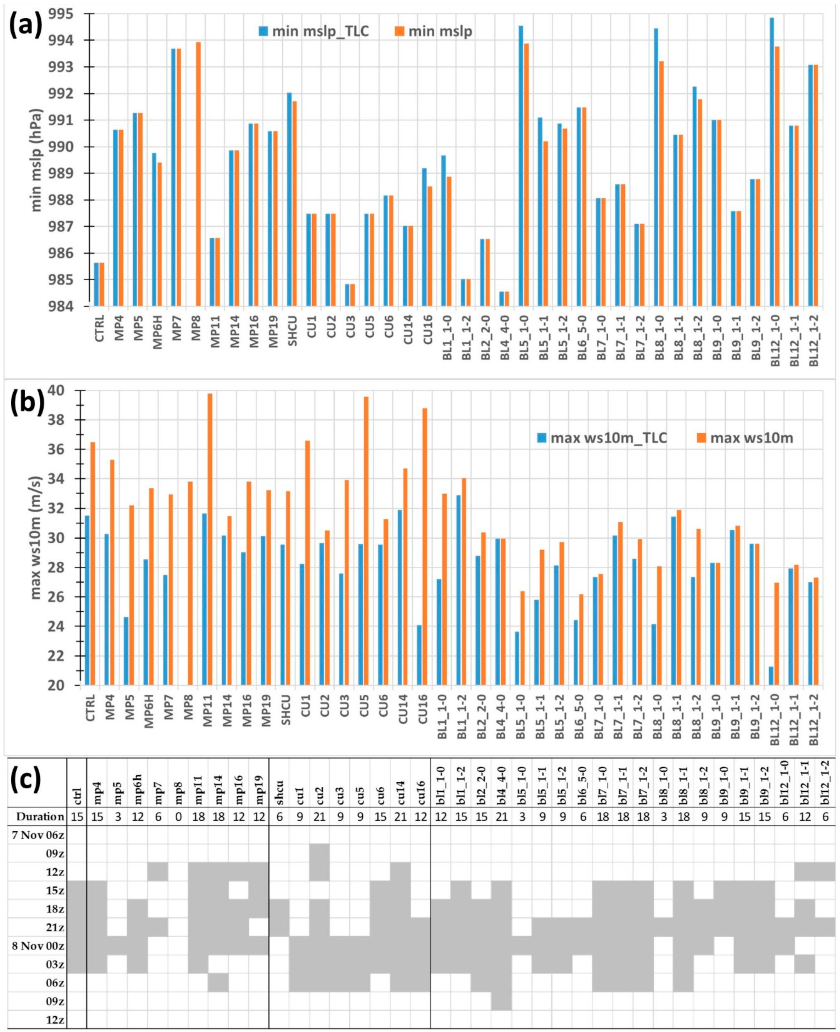
3.4. Aggregate Statistics

The main results regarding the intensity (in terms of minimum mslp and maximum 10-m wind speed (ws10m)) and the duration of a symmetric deep warm core (i.e., a medicane), are summarized in Figure 15 and

Table 2. The mean ± standard deviation of the minimum mslp (hPa), maximum 10-m wind speed (ws10m; m/s), track error (km), and duration of the medicane (hr) in the experiments with different microphysics (mp), cumulus (cu), and boundary/surface layer (bl) parameterizations. The last column presents the values of these parameters in ctrl. Mslp and ws10m are shown for the whole run (neglecting the first six hours of spin-up) and the medicane phase (TLC). The track error was calculated from the three-hour locations of the cyclone for the period 12:00 UTC 7 November 2014 to 00:00 UTC 8 November 2014. blC_1-0, blC_1-1, blC_1-2 (C=1, 5, 7, 8, 9, 12) correspond to all of the experiments with the revised MM5 surface layer scheme and isftcflx values equal to 0, 1, 2, respectively. Ctrl is included in the mp, cu, bl and blC_1-1 statistics.

Parameter	mp	cu	bl	blC_1-0	blC_1-1	blC_1-2	ctrl
min mslp	990.2 ± 2.6	987.6 ± 1.9	989.6 ± 2.8	991.5 ± 2.6	988.9 ± 2.0	989.4 ± 3.0	985.6
min mslp TLC	989.9 ± 2.4	987.7 ± 2.1	989.8 ± 3.1	992.1 ± 2.9	989.0 ± 2.2	989.5 ± 3.1	985.6
max ws10m	34.2 ± 2.4	35.0 ± 3.1	29.8 ± 2.6	28.4 ± 2.4	31.3 ± 2.9	30.2 ± 2.2	36.5
max ws10m TLC	29.3 ± 2.2	29.1 ± 2.3	27.9 ± 2.9	25.3 ± 2.7	29.6 ± 2.3	28.9 ± 2.1	31.5
track error	62.1 ± 25.6	81.6 ± 42.5	55.5 ± 24.2	48.9 ± 15.5	48.0 ± 19.3	67.5 ± 37.5	36.9
TLC duration	11.1 ± 6.17	13.0 ± 5.41	12.0 ± 5.37	8.5 ± 5.82	14.5 ± 3.51	12.0 ± 4.65	15

. The track errors, from 12:00 UTC 7 November 2014 to 00:00 UTC 8 November 2014, when the actual cyclone exhibited a symmetric deep warm core in the six-hour ECMWF analyses, have been provided in Figure 3, and are also summarized in Table 2.

The different parameterizations have resulted in a wide range of intensities and track errors. The minimum mslp usually occurred either during the medicane phase (in 66% of the runs; Figure 15a) within a few hours after the formation of the medicane, or some hours before, when at least a shallow warm core had formed in the lower troposphere. The control run attained a minimum mslp of 985.6 hPa, which was very close to the observed minimum of Malta (LMML; 984 hPa). Lower mslp was simulated only by bl4_4-0 (984.5 hPa), cu3 (984.8 hPa), and bl1_1-2 (985.0 hPa). Therefore, it seems that only a few modifications in the boundary/surface layer, cumulus scheme, or in the formulation of the surface fluxes of ctrl could produce a deeper cyclone that was closer to the observations.

On the other hand, the maximum ws10m was usually associated with the parent low, and was simulated in the medicane phase only in two out of the 38 experiments (Figure 15b). This happened because the wind speed depends on the pressure gradient, and not simply on the minimum mslp of the depression. In all of the experiments, the medicane reached a tropical storm speed (>17 m/s). The maximum ws10m during the medicane phase was predicted by bl1_1-2 (32.9 m/s; corresponding to a category 1 hurricane) and overall by mp11 (39.8 m/s). These values were close to the maximum gusts of 37.6 m/s, which were observed at Lampedusa island at the early stages of the observed medicane [8].

There was a large variability in the formation time and the duration of the medicane phase among the various experiments (Figure 15c). Most of the experiments formed a medicane at 12:00 or 15:00 UTC 7 November 2014. Cu2 produced the earliest development at 09:00 UTC 7 November 2014, while bl4_4-0 (with the lowest minimum mslp) was the only experiment that kept the medicane phase until 09:00 UTC 8 November 2014. The medicane duration ranged from three hours (in mp5, bl5_1-0, bl8_1-0) to 21 h (in cu2, cu14, bl4_4-0), while mp8 was the only experiment without the formation of a TLC.

About the trajectory, it was shown earlier in Section 3.1 that ctrl and its equivalent run with hail instead of graupel (mp6h) produced a track error of 36.9 km (Figure 3). The experiments bl9_1-2, bl9_1-1, and bl7_1-0 were the only ones that exhibited lower errors (of 30.9 km, 31.4 km, and 32.9 km, respectively). Therefore, a modification of the boundary/surface layer was necessary in order to perform a more accurate prediction of the track of the medicane, relative to ctrl.

The relationship between the track errors and the medicane’s duration and formation was investigated using the SST anomalies at the location of medicane’s formation (for each experiment) versus (a) the duration of the simulated medicane (Figure 16a) and (b) the delay in the formation of the simulated medicane relative to the actual one (Figure 16b). The experiment mp8, with the new Thompson microphysics, was not considered, because no medicane formed. The SST anomalies have been calculated relative to the SSTs (22.56 °C) at the location of the actual medicane’s formation (experiment minus 22.56), and have been averaged at a radius of 200 km around the minimum mslp of the cyclone. Figure 16 shows that there is a good linear correlation (R = 0.62, p < 0.01) between the SSTs at the location of medicane’s formation and the duration of the medicane. More importantly, there is a strong anticorrelation (R = −0.92, p < 0.01) between the SSTs at the location of the medicane’s formation and the delay of medicane formation relative to the actual system. The warmer the SSTs (or equivalently, the smaller the absolute SST anomalies), the longer the duration of the simulated medicane and the smaller the delay from the actual formation time. Therefore, the track errors determine the SSTs below the parent low and the medicane, and as a result, they influence the surface sensible and latent heat fluxes. The lack of medicane development in mp8 (in which the parent low encountered similar SSTs to the other experiments in most of its lifetime) and the occurrence of different medicane durations and delays despite the same SSTs in some experiments, suggest that other factors, such as the physical parameterizations, are also important for the formation and the duration of the simulated medicane. The physical parameterizations appear to affect the track of the parent low and the medicane, and thus, they influence the SSTs below the cyclone and the available energy input to the cyclone.

The largest variability of the minimum mslp and the maximum ws10m during the medicane phase, in terms of range (Figure 15) and standard deviation (3.1 hPa, 2.9 m/s), was exhibited by the bl experiments (Table 2). The different methods that were used to represent cumulus convection produced the largest mean (81.6 km) and standard deviation (42.5 km) in the track errors. The duration of the medicane seems to be influenced more strongly by the choice of the microphysics parameterization, which presented a standard deviation of 6.17 h (Table 2).

The option isftcflx seems to affect the intensity, track, and duration of the medicane and its parent low through the modification of the sea surface fluxes of energy (see blC_1-0, blC_1-1, and blC_1-2 in Table 2). Its influence on TLC14 was investigated in the experiments with the YSU boundary layer scheme and the revised MM5 parameterization. The lowest mean value (988.9 hPa, 989.0 hPa for TLC) and variability (2.0 hPa, 2.2 hPa for TLC) of the minimum mslp were produced when isftcflx was equal to one (Table 2). The same option produced the highest mean value of the maximum ws10m (31.3 m/s), the lowest mean track error (48.0 km), and the highest TLC duration (14.5 h), bringing it closer to the observed value. Despite the non-linearity in the development of tropical cyclones and medicanes, the stronger development by isftcflx equal to one rather than two is consistent with the larger exchange coefficients of sensible and latent heat in the former option (under neutral stability [29]).

Table 3. The mean, standard deviation, minimum, and maximum values of the minimum mslp (hPa), track error (km), and maximum distance of the various runs (km) in all of the experiments with different parameterizations (WRF) and the members of the ensemble prediction system of the ECMWF. Mslp is shown for the whole run after T+6 h (spin-up time). The track error (relative to the “best” track) and the maximum distance among the various runs were calculated at three-hour intervals from the locations of the cyclone for the period 12:00 UTC 7 November 2014 to 00:00 UTC 8 November 2014. The ECMWF statistics are based on 49 (out of the 51) ensemble members (including the control member).

Parameter	Mean	Standard Deviation	Minimum	Maximum
min mslp WRF	989.5	2.7	984.5	993.9
min mslp ECMWF	995.8	3.2	986.4	1001.2
track error WRF	64.4	30.7	30.9	176.7
track error ECMWF	139.5	54.7	62.8	309.0
max distance WRF	-	-	153.8	404.7
max distance ECMWF	-	-	543.1	589.1

provides a comparison of the ensembles created by the WRF experiments and the members of the Ensemble Prediction System (EPS) of the ECMWF, which was initialized at the same time as WRF (12:00 UTC 6 November 2014). Forty-nine (49) out of the 51 EPS members (including the control one) have been used, because the cyclone could not be tracked in two members. The ECMWF ensembles were available at three-hour intervals. The EPS produced a larger standard deviation (3.2 hPa) and range (14.8 hPa) than the WRF hindcasts (2.7 hPa and 9.4 hPa, respectively) in the minimum mslp. Despite the coarser resolution, one ECMWF member managed to predict a minimum mslp of 986.4 hPa, which was close to the minimum observed value of Malta. The corresponding ECMWF deterministic forecast of the minimum mslp was 989.3 hPa. Similarly, the ECMWF ensembles exhibited a larger error in their mean value (139.5 km) of the track error (relative to the “best” track) with a larger standard deviation (54.7 km) and range (246.2 km) than the WRF hindcasts. Regarding the spread of the locations of WRF and ECMWF EPS forecasts, the maximum distances among the members were calculated at three-hour intervals from 12:00 UTC 7 November to 00:00 8 November 2014. It is clear in Table 3 that the width of the WRF tracks (i.e. the maximum distance among them), which ranged from 153.8 km to 404.7 km, was systematically smaller (at all of the three-hour timesteps of the period of interest) than the one of the ECMWF. In general, the WRF ensemble produced smaller errors and variability than the ECMWF ensembles, which were based on a single model setup and perturbed initial conditions. However, it is recognized that the ECMWF ensemble predictions employed a much coarser horizontal resolution than WRF, and they were produced on a forecast mode, contrary to WRF, which was forced by analyses at its boundaries.

4. Summary and Conclusions

This study investigated the sensitivity of the simulations of a medicane, which appeared over central Mediterranean on 7–8 November 2014, to the microphysical, cumulus, and boundary/surface layer parameterizations.

All of the experiments, except from the one with the new Thompson microphysics, managed to develop a symmetric deep warm-core cyclone, corresponding to a medicane. It was shown that the existence of strong sea-surface fluxes of energy and latent heating were necessary for the development of a medicane that was similar to the observed one. There was a significant sensitivity of different aspects of the simulated medicane to the physical parameterizations. Different studies on tropical cyclones have pointed out the importance of physics parameterizations for a proper simulation [24,25,26,27,30]. This result agrees with Miglietta et al. [31], who investigated the influence of physics parameterizations on the simulation of the medicane of 26 September 2006 over southern Italy. However, in the present case (7–8 November 2014), the intensity of the simulated medicanes was mainly influenced by the boundary/surface layer scheme, the track by the representation of cumulus convection, and the duration of the symmetric deep warm core by the microphysical parameterization.

The incorporation of recent advances of tropical cyclone research in the calculation of the sea-surface fluxes, through the modification of the drag coefficient and the roughness lengths of heat and moisture, seems to improve the intensity, track, and duration of the medicane. It was one of the first times that the influence of the updated formulations of the surface fluxes was evaluated on a medicane.

The complexity of the microphysical scheme did not appear to lead to improvements in the medicane’s track. Relatively simple schemes may reproduce the track of the medicane adequately (in line with Miglietta et al. [31]).

The parameterization of shallow convection, with explicitly resolved deep convection, resulted in a weaker medicane with a shorter lifetime and delayed development of a symmetric deep warm core. The physical mechanism for this evolution was associated with the reduction of the moist static energy of the boundary layer due to shallow convection. This outcome agrees with the literature of tropical cyclones [78], but it is shown for the first time on a medicane.

In agreement with Miglietta et al. [31], an optimum combination of parameterizations that can simulate all of the characteristics of TLC14 does not seem to exist. The results of this study indicate that the control simulation, with explicitly resolved deep convection by a grid spacing of 7.5 km, was able to simulate TLC14 in satisfactory agreement with the available observations, producing a superior representation of the system relative to many other combinations of schemes, even with parameterized convection. The use of ensemble techniques, with higher resolution than the available global ensemble forecasts, may provide an effective way to improve their prediction. For example, the track error of the centroid of the mp, cu, bl, and all of the experiments, averaged from 12:00 UTC 7 November to 00:00 UTC 8 November 2014, was equal to 42.0 km, 53.9 km, 30.1 km, and 34.9 km, respectively.

It is recognized that this study deals with a single case, and some results may be case-dependent. More studies, focusing in particular on recent medicanes, are required in order to improve their representation by the modern numerical weather prediction models.

References

1. Michaelides, S.; Karacostas, T.; Sánchez, J.L.; Retalis, A.; Pytharoulis, I.; Homar, V.; Romero, R.; Zanis, P.; Giannakopoulos, C.; Bühl, J.; et al. Reviews and perspectives of high impact atmospheric processes in the Mediterranean. Atmos. Res. 2018, 208, 4–44. [Google Scholar] [CrossRef]
2. Emanuel, K. Genesis and maintenance of Mediterranean hurricanes. Adv. Geosci. 2005, 2, 217–220. [Google Scholar] [CrossRef]
3. Fita, L.; Flaounas, E. Medicanes as subtropical cyclones: The December 2005 case from the perspective of surface pressure tendency diagnostics and atmospheric water budget. Q. J. R. Meteorol Soc. 2018, 144, 1028–1044. [Google Scholar] [CrossRef]
4. Da Rocha, R.P.; Reboita, M.S.; Gozzo, L.F.; Dutra, L.M.M.; de Jesus, E.M. Subtropical cyclones over the oceanic basins: A review. Ann. N. Y. Acad. Sci. 2018. [Google Scholar] [CrossRef] [PubMed]
5. Miglietta, M.M.; Laviola, S.; Malvaldi, A.; Conte, D.; Levizzani, V.; Price, C. Analysis of tropical-like cyclones over the Mediterranean Sea through a combined modelling and satellite approach. Geophys. Res. Lett. 2013, 40, 2400–2405. [Google Scholar] [CrossRef]
6. Cavicchia, L.; von Storch, H.; Gualdi, S. A long-term climatology of medicanes. Clim. Dyn. 2014, 43, 1183–1195. [Google Scholar] [CrossRef]
7. Nastos, P.T.; Papadimou, K.K.; Matsangouras, I.T. Mediterranean tropical-like cyclones: Impacts and composite daily means and anomalies of synoptic patterns. Atmos. Res. 2018, 206, 156–166. [Google Scholar] [CrossRef]
8. Pytharoulis, I. Analysis of a Mediterranean tropical-like cyclone and its sensitivity to the sea surface temperatures. Atmos. Res. 2018, 208, 167–179. [Google Scholar] [CrossRef]
9. Winstanley, D. The north African flood disaster, September 1969. Weather 1970, 25, 390–403. [Google Scholar] [CrossRef]
10. Tous, M.; Romero, R. Meteorological environments associated with medicane development. Int. J. Climatol. 2013, 33, 1–14. [Google Scholar] [CrossRef]
11. Moscatello, A.; Miglietta, M.M.; Rotunno, R. Numerical analysis of a Mediterranean ‘hurricane’ over southeastern Italy. Mon. Weather Rev. 2008, 136, 4373–4397. [Google Scholar] [CrossRef]
12. Bauer, P.; Thorpe, A.; Brunet, G. The quiet revolution of numerical weather prediction. Nature 2015, 525, 47–55. [Google Scholar] [CrossRef] [PubMed]
13. Lagouvardos, K.; Kotroni, V.; Nickovic, S.; Jovic, D.; Kallos, G. Observations and model simulations of a winter subsynoptic vortex over the central Mediterranean. Meteorol. Appl. 1999, 6, 371–383. [Google Scholar] [CrossRef]
14. Pytharoulis, I.; Craig, G.C.; Ballard, S.P. Study of the hurricane-like Mediterranean cyclone of January 1995. Phys. Chem. Earth (B) 1999, 24, 627–632. [Google Scholar] [CrossRef]
15. Pytharoulis, I.; Craig, G.C.; Ballard, S.P. The hurricane-like Mediterranean cyclone of January 1995. Meteorol. Appl. 2000, 7, 261–279. [Google Scholar] [CrossRef] [Green Version]
16. Homar, V.; Romero, R.; Stensrud, D.J.; Ramis, C.; Alonso, S. Numerical diagnosis of a small, quasi-tropical cyclone over the western Mediterranean: Dynamical vs. boundary factors. Q. J. R. Meteorol. Soc. 2003, 129, 1469–1490. [Google Scholar] [CrossRef] [Green Version]
17. Davolio, S.; Miglietta, M.M.; Moscatello, A.; Pacifico, F.; Buzzi, A.; Rotunno, R. Numerical forecast and analysis of a tropical-like cyclone in the Ionian Sea. Nat. Hazards Earth Syst. Sci. 2009, 9, 551–562. [Google Scholar] [CrossRef] [Green Version]
18. Miglietta, M.M.; Moscatello, A.; Conte, D.; Mannarini, G.; Lacorata, G.; Rotunno, R. Numerical analysis of a Mediterranean “hurricane” over south-eastern Italy: Sensitivity experiments to sea surface temperature. Atmos. Res. 2011, 101, 412–426. [Google Scholar] [CrossRef]
19. Chaboureau, J.-P.; Pantillon, F.; Lambert, D.; Richard, E.; Claud, C. Tropical transition of a Mediterranean storm by jet crossing. Q. J. R. Meteorol. Soc. 2012, 138, 596–611. [Google Scholar] [CrossRef]
20. Tous, M.; Romero, R.; Ramis, C. Surface heat fluxes influence on medicane trajectories and intensification. Atmos. Res. 2013, 123, 400–411. [Google Scholar] [CrossRef]
21. Cioni, G.; Malguzzi, P.; Buzzi, A. Thermal structure and dynamical precursor of a Mediterranean tropical-like cyclone. Q. J. R. Meteorol. Soc. 2016, 142, 1757–1766. [Google Scholar] [CrossRef]
22. Miglietta, M.M.; Cerrai, D.; Laviola, S.; Cattani, E.; Levizzani, V. Potential vorticity patterns in Mediterranean “hurricanes”. Geophys. Res. Lett. 2017, 44, 2537–2545. [Google Scholar] [CrossRef]
23. Carrió, D.S.; Homar, V.; Jansa, A.; Romero, R.; Picornell, M.A. Tropicalization process of the 7 November 2014 Mediterranean cyclone: Numerical sensitivity study. Atmos. Res. 2017, 197, 300–312. [Google Scholar] [CrossRef]
24. Rao, D.V.B.; Prasad, D.H. Sensitivity of tropical cyclone intensification to boundary layer and convective processes. Nat. Hazards 2007, 41, 429–445. [Google Scholar] [CrossRef]
25. Li, X.; Pu, Z. Sensitivity of numerical simulation of early rapid intensification of Hurricane Emily (2005) to cloud microphysical and planetary boundary layer parameterizations. Mon. Weather Rev. 2008, 136, 4819–4838. [Google Scholar] [CrossRef]
26. Rambabu, S.; Vani, D.G.; Ramakrishna, S.S.V.S.; Rama, G.V.; Apparao, B.V. Sensitivity of movement and intensity of severe cyclone AILA to the physical processes. J. Earth Syst. Sci. 2013, 122, 979–990. [Google Scholar] [CrossRef]
27. Jin, Y.; Wang, S.; Nachamkin, J.; Doyle, J.D.; Thompson, G.; Grasso, L.; Holt, T.; Moskaitis, J.; Jin, H.; Hodur, R.M.; et al. The impact of ice phase cloud parameterizations on tropical cyclone prediction. Mon. Weather Rev. 2014, 142, 606–625. [Google Scholar] [CrossRef]
28. Quitián-Hernández, L.; Fernández-González, S.; González-Alemán, J.J.; Valero, F.; Martín, M.L. Analysis of sensitivity to different parameterization schemes for a subtropical cyclone. Atmos. Res. 2018, 204, 21–36. [Google Scholar] [CrossRef]
29. Green, B.W.; Zhang, F. Impacts of air–sea flux parameterizations on the intensity and structure of tropical cyclones. Mon. Weather Rev. 2013, 141, 2308–2324. [Google Scholar] [CrossRef]
30. Kepert, J.D. Choosing a boundary layer parameterization for tropical cyclone modeling. Mon. Weather Rev. 2012, 140, 1427–1445. [Google Scholar] [CrossRef]
31. Miglietta, M.M.; Mastrangelo, D.; Conte, D. Influence of physics parameterization schemes on the simulation of a tropical-like cyclone in the Mediterranean Sea. Atmos. Res. 2015, 153, 360–375. [Google Scholar] [CrossRef]
32. Pytharoulis, I.; Matsangouras, I.T.; Tegoulias, I.; Kotsopoulos, S.; Karacostas, T.S.; Nastos, P.T. Numerical study of the medicane of November 2014. In Perspectives on Atmospheric Sciences; Karacostas, T.S., Bais, A., Nastos, P.T., Eds.; Springer International Publishing: Basel, Switzerland, 2017; pp. 115–121. [Google Scholar]
33. Ricchi, A.; Miglietta, M.M.; Barbariol, F.; Benetazzo, A.; Bergamasco, A.; Bonaldo, D.; Cassardo, C.; Falcieri, F.M.; Modugno, G.; Russo, G.A.; et al. Sensitivity of a mediterranean tropical-like cyclone to different model configurations and coupling strategies. Atmosphere 2017, 8, 92. [Google Scholar] [CrossRef]
34. Skamarock, W.C.; Klemp, J.B.; Dudhia, J.; Gill, D.O.; Barker, D.M.; Duda, M.G.; Huang, X.Y.; Wang, W.; Powers, J.G. A description of the Advanced Research WRF Version 3. NCAR/TN-475+STR, USA. 2008, p. 113. Available online: http://www2.mmm.ucar.edu/wrf/users/docs/arw_v3.pdf (accessed on 31 August 2018).
35. Dimitriadou, K. Satellite Analysis of Tropical-Like Mediterranean Cyclones (Medicanes). Master’s Thesis, Aristotle University of Thessaloniki, Thessaloniki, Greece, 2017. (in Greek with English abstract). Available online: http://ikee.lib.auth.gr/record/294318/files/GRI-2017-20238 (accessed on 31 August 2018).
36. Wang, W.; Bruyère, C.; Duda, M.; Dudhia, J.; Gill, D.; Kavulich, M.; Keene, K.; Lin, H.-C.; Michalakes, J.; Rizvi, S.; et al. ARW version 3 Modeling System User’s Guide; National Center for Atmospheric Research—Mesoscale and Microscale Division: Boulder, CO, USA, 2016; p. 408. Available online: http://www2.mmm.ucar.edu/wrf/users/docs/user_guide_V3.7/ARWUsersGuideV3.7.pdf (accessed on 31 August 2018).
37. Chen, F.; Dudhia, J. Coupling an advanced land-surface-hydrology model with the Penn State-NCAR MM5 modeling system. Part I: Model implementation and sensitivity. Mon. Weather Rev. 2001, 129, 569–585. [Google Scholar] [CrossRef]
38. Iacono, M.J.; Delamere, J.S.; Mlawer, E.J.; Shephard, M.W.; Clough, S.A.; Collins, W.D. Radiative forcing by long-lived greenhouse gases: Calculations with the AER radiative transfer models. J. Geophys. Res. 2008, 113, D13103. [Google Scholar] [CrossRef]
39. Tegen, I.; Hollrig, P.; Chin, M.; Fung, I.; Jacob, D.; Penner, J. Contribution of different aerosol species to the global aerosol extinction optical thickness: Estimates from model results. J. Geophys. Res. 1997, 102, 23895–23915. [Google Scholar] [CrossRef] [Green Version]
40. Hong, S.Y.; Dudhia, J.; Chen, S.H. A revised approach to ice microphysical processes for the bulk parameterization of clouds and precipitation. Mon. Weather Rev. 2004, 132, 103–120. [Google Scholar] [CrossRef]
41. Rogers, E.; Black, T.; Ferrier, B.; Lin, Y.; Parrish, D.; DiMego, G. Changes to the NCEP Meso Eta Analysis and Forecast System: Increase in Resolution, New Cloud Microphysics, Modified Precipitation Assimilation, Modified 3DVAR Analysis; NOAA/NWS Technical Procedures Bulletin 488; Washington, DC, USA, 2001. Available online: http://www.emc.ncep.noaa.gov/mmb/mmbpll/mesoimpl/eta12tpb/ (accessed on 31 August 2018).
42. Hong, S.Y.; Lim, J.O.J. The WRF single-moment 6-class Microphysics Scheme (WSM6). J. Korean Meteorol. Soc. 2006, 42, 129–151. Available online: http://www.inscc.utah.edu/~u0758091/MPschemes/WSM6-hong_and_lim_JKMS.pdf (accessed on 31 August 2018).
43. Tao, W.K.; Simpson, J.; McCumber, M. An ice-water saturation adjustment. Mon. Weather Rev. 1989, 117, 231–235. [Google Scholar] [CrossRef]
44. Thompson, G.; Field, P.R.; Rasmussen, R.M.; Hall, W.D. Explicit forecasts of winter precipitation using an improved bulk microphysics scheme. Part II: Implementation of a new snow parameterization. Mon. Weather Rev. 2008, 136, 5095–5115. [Google Scholar] [CrossRef]
45. Neale, R.B.; Chen, C.C.; Gettelman, A.; Lauritzen, P.H.; Park, S.; Williamson, D.L.; Conley, A.J.; Garcia, R.; Kinnison, D.; Lamarque, J.F.; et al. Description of the NCAR Community Atmosphere Model (CAM5.0); Technical Note, NCAR/TN-486+STR; National Center for Atmospheric Research: Boulder, CO, USA, 2012; p. 289. [Google Scholar]
46. Lim, K.S.S.; Hong, S.Y. Development of an effective double-moment cloud microphysics scheme with prognostic Cloud Condensation Nuclei (CCN) for weather and climate models. Mon. Weather Rev. 2010, 138, 1587–1612. [Google Scholar] [CrossRef]
47. Mansell, E.R.; Ziegler, C.L.; Bruning, E.C. Simulated electrification of a small thunderstorm with two-moment bulk microphysics. J. Atmos. Sci. 2010, 67, 171–194. [Google Scholar] [CrossRef]
48. Hong, S.Y.; Park, H.; Cheong, H.B.; Kim, J.E.E.; Koo, M.S.; Jang, J.; Ham, S.; Hwang, S.O.; Park, B.K.; Chang, E.-C.; et al. The Global/Regional Integrated Model System (GRIMs). Asia-Pac. J. Atmos. Sci. 2013, 49, 219–243. [Google Scholar] [CrossRef]
49. Kain, J.S. The Kain-Fritsch convective parameterization: An Update. J. Appl. Meteorol. 2004, 43, 170–181. [Google Scholar] [CrossRef]
50. Janjic, Z.I. The step-mountain Eta coordinate model: Further developments of the convection, viscous sublayer, and turbulence closure schemes. Mon. Weather Rev. 1994, 122, 927–945. [Google Scholar] [CrossRef]
51. Janjic, Z.I. Comments on “Development and evaluation of a convection scheme for use in climate models”. J. Atmos. Sci. 2000, 57, 3686. [Google Scholar] [CrossRef]
52. Grell, G.A.; Freitas, S.R. A scale and aerosol aware stochastic convective parameterization for weather and air quality modeling. Atmos. Chem. Phys. 2014, 14, 5233–5250. [Google Scholar] [CrossRef] [Green Version]
53. Tiedtke, M. A comprehensive mass flux scheme for cumulus parameterization in large-scale models. Mon. Weather Rev. 1989, 117, 1779–1800. [Google Scholar] [CrossRef]
54. Han, J.; Pan, H.L. Revision of convection and vertical diffusion schemes in the NCEP Global Forecast System. Weather Forecast. 2011, 26, 520–533. [Google Scholar] [CrossRef]
55. Hong, S.Y.; Noh, Y.; Dudhia, J. A new vertical diffusion package with an explicit treatment of entrainment processes. Mon. Weather Rev. 2006, 134, 2318–2341. [Google Scholar] [CrossRef]
56. Jimenez, P.A.; Dudhia, J. Improving the representation of resolved and unresolved topographic effects on surface wind in the WRF model. J. Appl. Meteorol. Climatol. 2012, 51, 300–316. [Google Scholar] [CrossRef]
57. Sukoriansky, S.; Galperin, B.; Perov, V. Application of a new spectral theory of stably stratified turbulence to the atmospheric boundary layer over sea ice. Bound.-Lay. Meteorol. 2005, 117, 231–257. [Google Scholar] [CrossRef]
58. Nakanishi, M.; Niino, H. An improved Mellor-Yamada level-3 model: Its numerical stability and application to a regional prediction of advection fog. Bound.-Lay. Meteorol. 2006, 119, 397–407. [Google Scholar] [CrossRef]
59. Pleim, J.E. A combined local and nonlocal closure model for the atmospheric boundary layer. Part I: Model description and testing. J. Appl. Meteorol. Climatol. 2007, 46, 1383–1395. [Google Scholar] [CrossRef]
60. Bougeault, P.; Lacarrere, P. Parameterization of orography-induced turbulence in a mesobeta-scale model. Mon. Weather Rev. 1989, 117, 1872–1890. [Google Scholar] [CrossRef]
61. Bretherton, C.S.; Park, S. A new moist turbulence parameterization in the Community Atmosphere Model. J. Clim. 2009, 22, 3422–3448. [Google Scholar] [CrossRef]
62. Grenier, H.; Bretherton, C.S. A moist PBL parameterization for large-scale models and its application to subtropical cloud-topped marine boundary layers. Mon. Weather Rev. 2001, 129, 357–377. [Google Scholar] [CrossRef]
63. Jimenez, P.A.; Dudhia, J.; Gonzalez-Rouco, J.F.; Navarro, J.; Montavez, J.P.; Garcia-Bustamante, E. A revised scheme for the WRF surface layer formulation. Mon. Weather Rev. 2012, 140, 898–918. [Google Scholar] [CrossRef]
64. Fairall, C.W.; Bradley, E.F.; Hare, J.E.; Grachev, A.A.; Edson, J.B. Bulk parameterization of air-sea fluxes: Updates and verification for the COARE algorithm. J. Clim. 2003, 16, 571–591. [Google Scholar] [CrossRef]
65. Donelan, M.A.; Haus, B.K.; Reul, N.; Plant, W.J.; Stiassnie, M.; Graber, H.C.; Brown, O.B.; Saltzaman, E.S. On the limiting aerodynamic roughness of the ocean in very strong winds. Geophys. Res. Lett. 2004, 31, L18306. [Google Scholar] [CrossRef]
66. Powell, M.D.; Vickery, P.J.; Reinhold, T.A. Reduced drag coefficient for high wind speeds in tropical cyclones. Nature 2003, 24, 395–419. [Google Scholar] [CrossRef] [PubMed]
67. Garratt, J.R. The Atmospheric Boundary Layer; Cambridge University Press: Cambridge, UK, 1992; p. 316. [Google Scholar]
68. Rizza, U.; Canepa, E.; Ricchi, A.; Bonaldo, D.; Carniel, S.; Morichetti, M.; Passerini, G.; Santiloni, L.; Puhales, F.S.; Miglietta, M.M. Influence of wave state and sea spray on the roughness length: Feedback on medicanes. Atmosphere 2018, 9, 301. [Google Scholar] [CrossRef]
69. Hart, R.E. A cyclone phase space derived from thermal wind and thermal asymmetry. Mon. Weather Rev. 2003, 131, 585–616. [Google Scholar] [CrossRef]
70. Evans, J.L.; Hart, R.E. Objective indicators of the life cycle evolution of extratropical transition for Atlantic tropical cyclones. Mon. Weather Rev. 2003, 131, 909–925. [Google Scholar] [CrossRef]
71. Wang, T. An explicit simulation of tropical cyclones with a triply nested movable mesh primitive equation model: TCM3. Part II: Model refinements and sensitivity to cloud microphysics parameterization. Mon. Weather Rev. 2002, 130, 3022–3036. [Google Scholar] [CrossRef]
72. Pytharoulis, I. Numerical study of the transformation of African easterly waves into tropical cyclones in north Atlantic. In Proceedings of the 23rd conference on Hurricanes and Tropical meteorology, Dallas, TX, USA, 10–15 January 1999; American Meteorological Society: Boston, MA, USA; pp. 925–928. [Google Scholar]
73. Emanuel, K.A. An air-sea interaction theory for tropical cyclones. Part I: Steady-state maintenance. J. Atmos. Sci. 1986, 43, 585–604. [Google Scholar] [CrossRef]
74. Schubert, W.H.; Hack, J.J.; Silva Dias, P.L.; Fulton, S.R. Geostrophic adjustment in an axisymmetric vortex. J. Atmos. Sci. 1980, 37, 1464–1484. [Google Scholar] [CrossRef]
75. Rodts, S.M.A.; Duynkerke, P.G.; Jonker, H.J.J. Size distributions and dynamical properties of shallow cumulus clouds from aircraft observations and satellite data. J. Atmos. Sci. 2003, 60, 1895–1912. [Google Scholar] [CrossRef]
76. Torn, R.D.; Davis, C.A. The influence of shallow convection on tropical cyclone track forecasts. Mon. Weather Rev. 2012, 140, 2188–2197. [Google Scholar] [CrossRef]
77. O’Shay, A.J.; Krishnamurti, T.N. An examination of a model’s components during tropical cyclone recurvature. Mon. Weather Rev. 2004, 132, 1143–1166. [Google Scholar] [CrossRef]
78. Zhu, H.; Smith, R.K. The importance of three physical processes in a minimal three-dimensional tropical cyclone model. J. Atmos. Sci. 2002, 59, 1825–1840. [Google Scholar] [CrossRef]
79. Zhu, H.; Smith, R.K.; Ulrich, W. A minimal three-dimensional tropical cyclone model. J. Atmos. Sci. 2001, 58, 1924–1944. [Google Scholar] [CrossRef]
Figure 1. The sea-surface temperatures (°C; valid on 6 November 2014) and the domain used by all of the Weather Research and Forecasting (WRF) experiments. The “best” track of the parent low (black line), the tropical-like cyclone (defined as a symmetric deep warm-core system; red line) and the cyclone that remained after it lost its tropical-like features (black line) is illustrated from 00:00 UTC 7 November 2014 to 00:00 UTC 9 November 2014. Star: 12:00 UTC 7 November, square: 18:00 UTC 7 November, rhombus: 00:00 UTC 8 November and circle: 06:00 UTC 8 November. The dots are depicted in 3-h intervals from 12:00 UTC 7 November to 06:00 UTC 8 November, and in 6-h intervals elsewhere.
Atmosphere 09 00436 g001
Figure 2. The track of the intense tropical-like cyclone (TLC) that formed south of Sicily on 7 November 2014 (TLC14), its parent low, and the cyclone that remained after TLC14 lost its tropical characteristics in the WRF experiments: (a) ctrl, mp4, mp5, mp6h, mp7, mp8, and (b) ctrl, mp11, mp14, mp16 and mp19, at three-hour intervals from 00:00 UTC 7 November 2014 to 00:00 UTC 9 November 2014. The “best track” of the actual systems is also illustrated. Star: 12:00 UTC 7 November 2014, square: 18:00 UTC 7 November 2014, rhombus: 00:00 UTC 8 November 2014, and circle: 06:00 UTC 8 November 2014.
Atmosphere 09 00436 g002
Figure 3. The mean distance (km) of the three-hour locations of TLC14, its parent low, and the cyclone that remained after TLC14 lost its tropical characteristics in the WRF experiments from the “best” track, averaged from 12:00 UTC 7 November 2014 to 00:00 UTC 8 November 2014.
Atmosphere 09 00436 g003
Figure 4. Time series of the minimum mslp (hPa) of the TLC14, its parent low, and the cyclone that remained after TLC14 lost its tropical characteristics in the WRF experiments (in hourly intervals) with different: (a) microphysical, (b) cumulus, and (c) boundary/surface layer schemes, in the European Centre for Medium Range Weather Forecasts (ECMWF) analyses (six-hour) and at the airport of Malta (LMML) at 16:34 UTC on 7 November 2014.
Atmosphere 09 00436 g004
Figure 5. Phase space diagrams of V T L (900–600 hPa) vs. V T U (600–300 hPa) in the WRF experiments ctrl, mp4, mp5, mp6h, mp7, mp8, mp11, mp14, mp16, and mp19, at three-hour intervals. The diagrams have been calculated using a radius of 200 km around the three-hour locations of the cyclone’s minimum mean sea-level pressure (mslp). The red squares denote the times when the symmetry/asymmetry parameter B was less than 10 m. Circle: 18:00 UTC 6 November 2014. Open squares: UTC time and date (7–9 November 2014) at 12-h intervals starting at 00:00 UTC 7 November 2014 (00z7).
Atmosphere 09 00436 g005
Figure 6. Hovmoller diagrams of microphysics latent heating (K·h−1) in the WRF experiments (a) ctrl, (b) mp8, and (c) mp11, at hourly intervals, averaged within a radius of 200 km around the location of the cyclone’s minimum mslp.
Atmosphere 09 00436 g006
Figure 7. As for Figure 2, but for the WRF experiments: (a) ctrl, shcu, cu1, cu2, cu3 and (b) ctrl, cu5, cu6, cu14, cu16, together with the best track of the observed cyclone.
Atmosphere 09 00436 g007
Figure 8. Horizontal sections of geopotential height (gpm; contours) and wind vectors (every eighth grid point for clarity) at 850 hPa at 06:00 UTC 7 November 2014 in the WRF experiments (a) ctrl and (b) shcu. The vector at the bottom corresponds to a wind speed of 40 m/s.
Atmosphere 09 00436 g008
Figure 9. As for Figure 5, but for the WRF experiments shcu, cu1, cu2, cu3, cu5, cu6, cu14, and cu16.
Atmosphere 09 00436 g009
Figure 10. Hovmoller diagrams of heating (K·h−1) from the microphysics scheme in (a) cu3, (b) shcu, and (c) from the cumulus scheme in cu3, at hourly intervals, averaged within a radius of 200 km around the location of the cyclone’s minimum mslp.
Atmosphere 09 00436 g010
Figure 11. Hovmoller diagrams of (a) moistening rate (g·kg−1·h−1), (b) heating rate (K·h−1), and (c) moist static energy rate of change (J·kg−1·h−1) due to the terms Cp·(∂T/∂t) + Lv·(∂q/∂t), from the shallow convection scheme in shcu, at hourly intervals, averaged within a radius of 200 km around the location of the cyclone’s minimum mslp. Cp, Lv T, q, and t correspond to the specific heat of air at constant pressure, the latent heat of vaporization, temperature, mixing ratio, and time, respectively. The same color scale is used in panels (a,b).
Atmosphere 09 00436 g011
Figure 12. As for Figure 2, but for the WRF experiments: (a) ctrl, bl1_1-0, bl1_1-2, bl2_2-0, bl4_4-0, (b) ctrl, bl5_1-0, bl5_1-1, bl5_1-2, bl6_5-0, (c) ctrl, bl7_1-0, bl7_1-1, bl7_1-2, (d) ctrl, bl8_1-0, bl8_1-1, bl8_1-2, (e) ctrl, bl9_1-0, bl9_1-1, bl9_1-2 and (f) ctrl, bl12_1-0, bl12_1-1, bl12_1-2, together with the best track of the observed cyclone.
Atmosphere 09 00436 g012
Figure 13. As for Figure 5, but for the WRF experiments with the different boundary/surface layer parameterizations.
Atmosphere 09 00436 g013aAtmosphere 09 00436 g013b
Figure 14. Time series of (a) sea-surface temperatures (SST; °C) and (b) surface latent (LH; solid lines) and sensible (SH; dotted lines) heat fluxes (W/m2), averaged in a radius of 200 km around the minimum mean sea-level pressure (mslp) of the cyclone, at these experiments ctrl, bl4_4-0, and bl12_1-0.
Atmosphere 09 00436 g014
Figure 15. (a) The minimum mslp (hPa) and (b) the maximum 10-m wind speed (ws10m; m/s) in a radius of 200 km around the minimum mslp, of the cyclone in the whole run (after six hours of spin-up time) (orange columns) and during the TLC phase (blue columns) at each WRF experiment. (c) The period and the total duration (hr) of the TLC phase at each WRF experiment.
Atmosphere 09 00436 g015
Figure 16. Scatter plots of the SST anomalies at the location of medicane’s formation (at each experiment) versus (a) the duration of the simulated medicane and (b) the delay in its formation relative to the actual one. Positive (negative) values of “delay” correspond to a later (an earlier) formation of the simulated medicane than the actual one. The SST anomalies have been calculated relative to the SSTs at the location of the actual medicane’s formation (experiment minus 22.56), and have been averaged at a radius of 200 km around the minimum mslp of the cyclone. The best fit line, the linear correlation coefficient (R), and the determination coefficient (R2) are also provided.
Atmosphere 09 00436 g016