1. Introduction
Rainfall-runoff is an important hydrological process that affects many different types of environmental factors including soil, topography, vegetation, and natural resources within catchments. Runoff studies are often dependent on the characteristics of natural rainfall such as its variability in intensity, spatio-temporal distribution, drop size distribution, drop velocity, and kinetic energy [
1]. Rainfall simulation is the prevalent method applied in hydrogeomorphological studies that include runoff, infiltration, soil characteristics in catchments, and other study areas for replicating the features and processes of natural rainfall [
2].
A rainfall simulator (RS) is widely used as research tool to produce runoff, infiltration, and erosion data in field- and laboratory-based studies of hydrological and geomorphological processes [
3,
4,
5,
6]. The main purpose of an RS is to provide a reproducible collection of rainfall data as well as to accurately and precisely create a variety of rainfall regimes by controlling the rainfall intensity and duration [
2,
7,
8]. The data collected from rainfall simulation experiments provide fundamental information to understand the dynamic behaviors of runoff generation, infiltration and soil erosion; this information is focused on how surface properties such as slope, soil properties, vegetation cover, and topography within catchments impact the above-mentioned processes [
9,
10].
There is no universal RS applicable to all study conditions [
5,
9]. Many different types of RSs have been developed to study various components of hydrological and geomorphological processes through the artificial reproduction of rainfall [
5,
11,
12]. RSs can be classified into two main groups according to the method through which the drop-forming mechanism creates rain [
3,
6,
8,
11]. The first group consists of the non-pressurized drop-forming simulators, where the raindrops are formed at the tip of a conduit (i.e., drop former), such as needles connected to a set of pipes, or directly from holes in the base of a tank. The drop formers initiate the fall of drops with zero velocity. The second group consists of pressurized nozzle simulators, where the raindrops are continuously produced by single or multiple nozzles at significant velocities.
Non-pressurized drop-forming simulators have limitations in reproducing natural rainfall in terms of drop size and energy characteristics [
2,
8,
11,
13]. These types of simulators generally provide uniformly distributed raindrops in terms of size; however, they do not produce a distribution of drops unless various sizes or dimensions of drop formers are used. Another shortcoming of the non-pressurized drop-forming simulators is the limited application to soil erosion studies, particularly in field experiments. These simulators are usually impractical for field use because a sufficient height from the impact surface is needed for raindrops to reach terminal velocity corresponding with rainfall kinetic energy.
By contrast, the pressurized nozzle simulators produce wider drop-size distributions. A variety of nozzle types can be employed in rainfall simulation, and drop-size distributions are governed by the shape features and discharge of the nozzle. These types of simulators also provide a variety of storm intensities [
13,
14]. Rainfall intensities can be varied with nozzle orifice, pump pressure, nozzle spacing, and nozzle movements. While these simulators provide reasonable velocities and kinetic energy values of raindrops at low fall heights, droplet velocities are generally exaggerated because the raindrops from nozzles have an initial velocity greater than zero due to the pump pressure forcing them out. The continuous spray from the nozzles may also lead to higher rainfall intensities than natural rainfall. A rotating disc, a rotating boom, an oscillating bar, or a solenoid-controlled simulator can be used as the solution to reduce the exaggerated rainfall intensity [
2,
8,
15]. A rotating or oscillating bar is the simplest method of closely simulating natural rainfall in terms of rainfall intensities [
16]. Boxes around nozzles to regulate sprayed raindrops are also introduced to decrease rainfall intensity higher than that of natural rainfall by reducing the time of surface exposure to the artificial rain spray [
8].
There are also indoor and outdoor RSs according to transportability [
7]. Small, portable field RSs can be useful due to their easy and rapid transport and implementation, but the small size generally limits their applications to accurate assessment of the net runoff response, including heterogeneity in surface properties at the plot scale [
10]. On the other hand, laboratory RSs have been used to overcome the disadvantages of the small, portable field RSs [
2,
7]. Laboratory RSs prevent the disruptive impacts of wind, temperature, and humidity on experiments [
17].
Recently, research has focused more on the assessment of the effects of surface property changes resulting from fire, agriculture, urbanization or other disturbances on the hydrologic cycle [
18,
19,
20,
21,
22,
23,
24]. These studies include broad experiments that evaluate the characteristics of the land surface on a scale from a hillslope to a catchment to further understand the interplay between surface properties and runoff generation. This requires a laboratory RS that is sufficiently large to produce high rainfall intensities and that is suited to capture heterogeneity of surface properties across an experimental surface. Such measurements from a large laboratory RS can be used to increase the runoff response accuracy and precision of hydrological models [
10]. Although additional research using large laboratory RSs is needed to assess the effects of surface property changes on the hydrologic cycle, simple and small RSs that produce rain over small areas (less than 5 m
2 and mostly less than 1 m
2) have been widely used [
5,
12,
25,
26,
27,
28,
29,
30,
31,
32]. This is due to the fact that RSs covering relatively large areas (approximately 100 m
2 or more) are expensive to set up and are not easy to operate [
2].
For accurate runoff experiments, the RSs should adequately simulate natural rainfall and control the intensity and duration of the rainfall. In addition to the desirable characteristics for precisely simulating rainfall, RSs need other requirements such as efficiency, simplicity, and economy [
33]. However, it is difficult to meet the all requirements for RSs because there is a trade-off among the desirable characteristics such as size, cost, portability, areal coverage, ease of use, and operation [
10,
11,
34]. The desirable features of RSs primarily depend on the research objectives and the rainfall characteristics required for specific research conditions.
In the case of large indoor RSs, major requirements for runoff experiments include reliability and accuracy. Reliability is associated with the repeatability of storm events, and accuracy relates to spatial uniformity in rainfall over the entire test plot [
8]. A reproducible rainfall pattern can be provided more reliably when the desired intensities and duration of the storm are controlled by the computer-driven operation system. This removes the problems related to human errors in changing the storm pattern. The reliability can also be enhanced by implementing appropriate instrumentation that correctly monitors storm events across the test plot. Accuracy is evaluated by the degree of uniformity of rainfall distribution over the test plot. The accuracy can be increased or at least be as high as possible when an adequate spray nozzle type is chosen and nozzles are placed in series with adequate spacing to ensure even overlap of raindrops. Additionally, the physical movement of the nozzles back and forth across an experimental plot can have notable effects on the uniformity of rainfall distribution [
8].
In general, the depths and spatial distribution of rainfall are manually measured with collection containers equally distributed over an entire experimental plot to provide quantitative information on the reproducibility and homogeneity of rainfall. The mass of water collected in each container during an experiment is converted to rainfall depth per hour, and then the mean simulated rainfall intensities are calculated. The spatial homogeneity of a certain rainfall event is mostly evaluated using the Christiansen uniformity coefficient (CuC) [
35]. This type of experiment is repeated for different rainfall intensities and for different runs at the same intensity.
These traditional measurements are widely used for small-scale rainfall simulation, while manual procedures are not suitable for relatively large experimental areas (100 m
2 or more) because of the inefficiency in terms of the time and human resources required to cover large areas. The intensity and spatial distribution of rainfall are controlled by a combination of the variables of an RS system, such as the orifice diameter of the nozzle, the pressure at the nozzle and the nozzle movement (e.g., the oscillation speed of bars and the time delay at the end of each oscillation). The larger the RS, the more system variables the RS has, and hence the more difficult it is to fit the target intensity for a specified time period having a reasonable uniformity of rainfall distribution because of the increased number of combinations in the RS’s system variables. In addition, traditional measurement based on manual procedures has its own sources of errors due to human mistakes. These measurement errors vary randomly in magnitude under the same conditions of the RS’s system variables. If errors in rainfall intensity generated from an RS are not considered before use in analysis, the researchers could draw erroneous conclusions regarding the study objective, such as infiltration, pavement effects in urbanized areas, and storage capacity of catchments [
36].
In addition, a variety of rainfall simulators have been calibrated over an experimental area, often with little consideration of issues such as interrelationships of the system variables of the RS and the intensity and uniformity distribution of rainfall. In particular, in a large RS, limited attention is placed on the identification of relationships between the system variables of the RS and the intensity and uniformity distribution of rainfall, even though those relationships are very important to produce and replicate a steady supply of rainfall at a fixed and known intensity, and there are also increasing issues related to the use of a large RS in hydrogeomorphological studies. To overcome the limitations caused by manual measurements to obtain the rainfall intensity and spatial rainfall distribution in a large experimental area, an additional device is required. The main purpose of this study is to establish a method to calibrate a large-scale laboratory rainfall simulator through developing and implementing an automated rainfall collection system (ARCS) to assess the reliability and accuracy of a rainfall simulator. The ARCS is implemented to identify functional relationships between the system variables of the RS and the intensity and uniformity distribution of rainfall (i.e., operation models). The operation models can be used as a guideline to intuitively select appropriate ranges of the system variables of the rainfall simulator to generate a particular rainfall intensity and degree of uniformity for simulated rainfall in laboratory-based studies of hydrological and geomorphological processes.
2. Large-Scale Laboratory Rainfall Simulator
The large-scale laboratory RS of the NDMI (National Disaster Management Research Institute) reproduces spatially uniform rainfall with an oscillating nozzle system for experimental areas up to 900 m
2. The RS is a pressurized nozzle-type simulator with computer-operated oscillating booms. The NDMI RS consists of several parts: an underground water storage tank (900 m
3), submersible pumps (0.25 m
3/s × 4 pumps), a rooftop water storage tank (63 m
3), a water supply system (from submersible pumps to nozzles), booster pumps (1.7 m
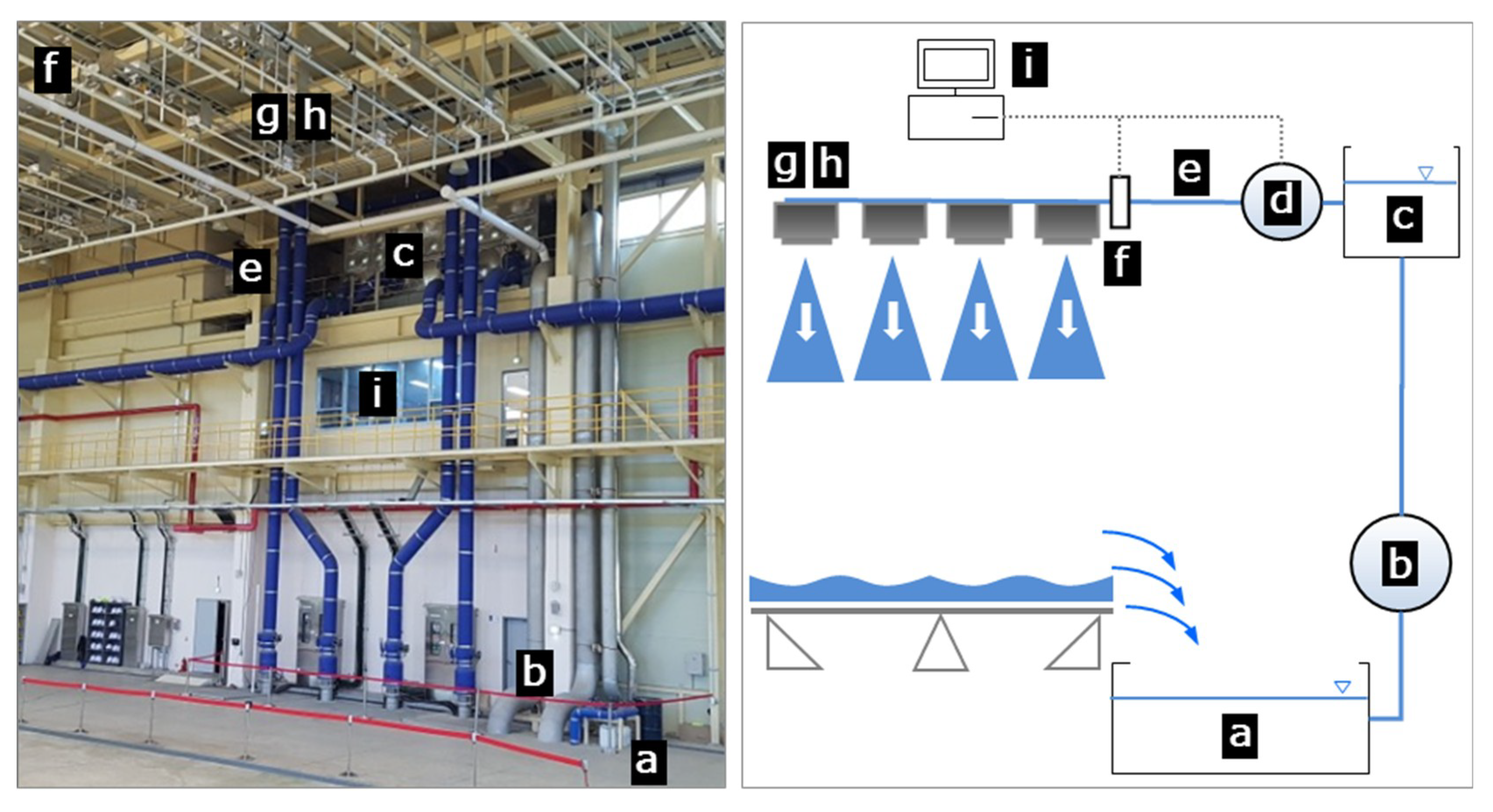
3/min × 3 pumps), computer-driven motors (to control oscillating pipes with nozzles), nozzles, spray boxes, and a computer-controlled operating system. Submersible pumps provide water from the underground storage tank below the laboratory to the rooftop storage tank. Water from the rooftop storage tank is supplied to each nozzle of the RS through the water delivery system. The booster pumps control the inflow of water from the rooftop storage tank to the water supply system, keeping the pressure constant and ensuring each nozzle has the similar (or the same) discharge rate. Through a drainage system on the ground, the raindrops released by nozzles are re-collected in the underground storage tank for reuse.
Figure 1 shows the inside view of the NDMI RS laboratory and a schematic diagram of the water circulation process in the NDMI RS.
The size of the RS is 30 m (length) by 30 m (width). The simulator and its experimental area can be divided into nine different sub-sections (10 × 10 m) that can be operated independently, which enables efficient experiments ranging from small-scale models to actual-size testing. The simulator’s nozzles are at a height of 12 m above the ground to ensure the terminal speed of raindrops. Four sets of nozzles are installed and equally spaced at a 2.5-m distance along the pipelines of the sub-section. Each set consists of two nozzles. The nozzle type is KJ 80150 (an orifice diameter of 7.5 mm with a flat fan spray type). The configuration of the nozzles is presented in
Figure 2.
The spray boxes beneath each pair of oscillating nozzles are used to reduce rainfall intensity by cutting off the spray. Details of the spray box structure are given in
Figure 3. There are 144 spray boxes installed throughout the whole RS (see
Figure 2). In general, the oscillating-nozzle system without spray boxes enables adjustment of simulated rainfall characteristics by changing the nozzle type used, the water pressure at the nozzle and the sweep oscillation frequency of the nozzles. In the case of the oscillating-nozzle system with spray boxes, the variables that control nozzle movement, which affects the intensity and uniformity of rainfall, are not only related to the velocity of oscillating nozzles across the spray box but also the time delay at the outside of the central square opening in the spray box. With nozzles located at the corner of the spray box, the water spray does not go through the central square hole of the spray box but is transferred through the gutter that transports water back to the underground storage tank.
In the NDMI RS, the nozzle pressure (NP) ranges from 1.3 to 7.0 kg/cm2 with an increment of 0.1, yielding flow rates of 0.96 to 3.91 m3/min. The oscillation velocity (OV) of nozzles varies from 6.25 to 31.25 rpm with an increment of 1.25 rpm, and the time delay (TD) of nozzles in the spray boxes varies from 0 to 10 s with an increment of 0.1 s. The system variables such as the NP, the OV, and the TD can be automatically changed using the computer-controlled operation system.
4. Results
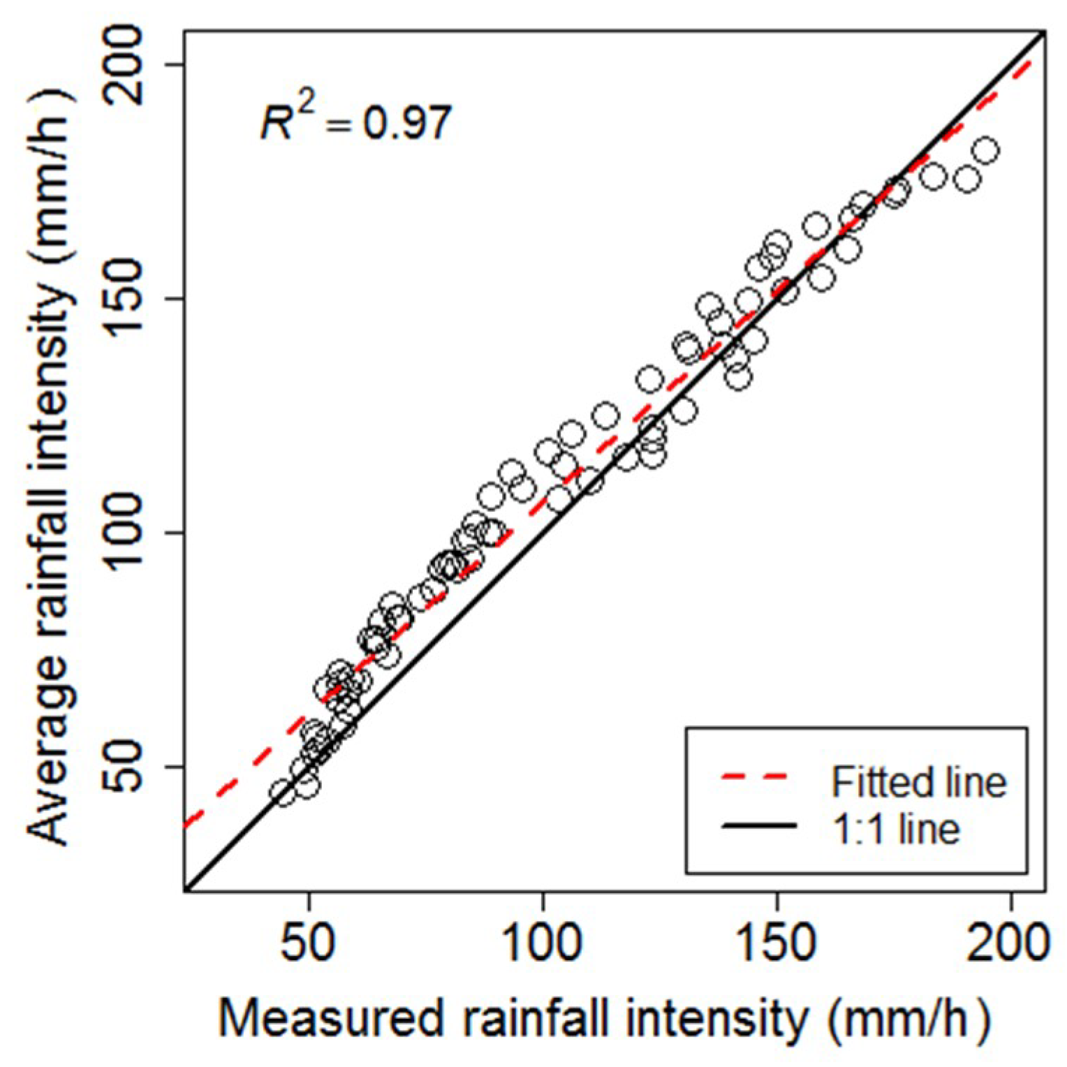
The RS has been calibrated for the rainfall intensity and the uniformity of rainfall distribution at various combinations of the system variables: the operating pressures and the oscillatory movements including velocity and time delay. Before assessing the reliability and accuracy of the RS based on calibration results, the adequacy of the average rainfall intensities (I
average) from rain gauges for all system variables was evaluated through a graphical comparison with those measured by the flowmeter (I
total). As shown in
Figure 5, the interaction points between I
average and I
total were evenly distributed on both sides of the 1:1 line in the relatively high rainfall range from 130 to 200 mm/h, while I
average was slightly overestimated for the rainfall range from 60 to 130 mm/h. However, the average rainfall intensities generally showed good agreement with the total rainfall intensities measured by the flowmeter. The fitted line between the values from I
average and I
total was very close to the 1:1 correspondence. The performance statistic also shows that I
average exhibited high accuracy in estimating rainfall intensities (an
R2 of 0.97 between the I
average and I
total values).
Sousa Junior et al. [
36] estimated the average rainfall intensities using two different methods. One was the traditional manual measurement (63 collection cans arranged in a 7 × 9 mesh spaced 0.25 m apart in a 3-m
2 area). The other was a volumetric method in which the total amount of rainfall collected in a container (3 m
2) was measured. These authors compared the rainfall intensities from two methods for rainfall ranging from 170 to 250 mm/h. The average rainfall intensities calculated from the traditional measurement were generally overestimated. There was a large difference in average rainfall intensities ranging from 170 to 200 mm/h (the deviation between the values from the two methods was approximately 30~35 mm/h), while in this study, the difference between I
average and I
total was approximately 2~7 mm/h for the same rainfall range.
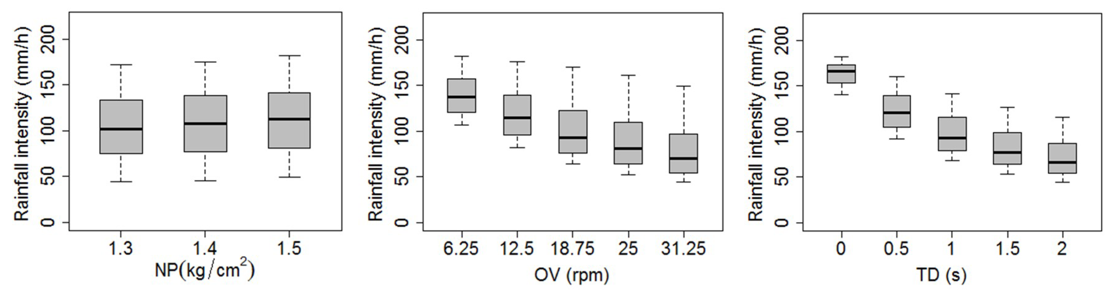
The variability of the average rainfall intensity (hereinafter rainfall intensity) in response to the three system variables (i.e., based on 75 combinations of NP, OV, and TD) is compared in
Table 1 and
Figure 6.
Table 1 provides a summary of statistics of the calibration results for the rainfall intensity for each system variable, and the variability in the rainfall intensity for each system variable is visually compared using box-and-whisker diagrams in
Figure 6. The RS provided rainfall intensities between 44.1 and 181.7 mm/h for the three system variables (
Figure 6). As shown in
Figure 6, a similar range of rainfall intensity was produced across all of the operating pressures (NP values of 1.3, 1.4 and 1.5 kg/cm
2). The average rainfall intensity increased slightly with increasing NP (an average of 104.5, 108.4 and 112.1 mm/h in response to NP values of 1.3, 1.4 and 1.5 kg/cm
2, respectively;
Table 1), but no substantial difference was detected with an increase in the NP value. By contrast, increases in the OV and TD values significantly decreased the rainfall intensity (the mean ranged from 82.6 to 140.5 mm/h and from 72.8 to 162.6 mm/h in response to OV and TD, respectively;
Table 1). The lower the OV and TD, the higher the rainfall intensity of the RS.
A summary of statistics of the calibration results for the spatial rainfall uniformity is shown in
Table 2, and
Figure 7 presents the range of the CuC values calculated in response to changes in the three system variables. The uniformity coefficient for all cases ranged between 70.1% (for NP of 1.3 kg/cm
2, OV of 31.25 rpm and TD of 2.0 s, which resulted in a rainfall intensity of 44.1 mm/h) and 78.4% (for NP of 1.5 kg/cm
2, OV of 6.25 rpm and TD of 0.0 s, which resulted in a rainfall intensity of 181.7 mm/h). The uniformity coefficient was influenced primarily by the change in NP and OV. The CuC values of simulated rainfall improved with an increase in NP, and the RS yielded higher values of uniformity coefficients at an NP value of 1.5 kg/cm
2 (CuC values ranged from 74.2 to 78.4% in
Figure 7, with rainfall intensities ranging from 49.1 to 181.7 mm/h in
Figure 6). The spatial distributions of the simulated rainfall appeared to be improved with a decrease in OV. An increase in OV was inversely proportional to both the rainfall intensity and the uniformity coefficient (
Figure 6 and
Figure 7), whereas the uniformity coefficient was not significantly affected by changes in TD. A sample plot for the spatial rainfall distribution (rainfall intensity of 181.7 mm/h and CuC of 78.4%) is presented in
Figure 8. The overall spatial pattern of distributions for other rainfall intensities was broadly similar in terms of zones of high and low rainfall amounts despite the changing rainfall intensities.
The calibration results for the rainfall intensity and the spatial rainfall uniformity in response to each system variable revealed that OV had a strong relationship with both the rainfall intensity and the uniformity coefficient at the same time. Higher uniformity was also observed in response to an NP of 1.5 kg/cm2, which included the whole range of rainfall intensities yielded from all combinations of the RS’s system variables (NP, OV, and TD). In this study, the operation models of the RS were derived under the pressure condition (NP of 1.5 kg/cm2) that had the highest level of spatial rainfall uniformity and included the range of rainfall intensities for all combinations of the three system variables, according to interrelationships between the system variables in the RS and the intensity and uniformity distribution of rainfall.
Figure 9 represents scatter plots of the OV for each TD (i.e., 0.0, 0.5, 1.0, 1.5, and 2.0 s) against the intensity and uniformity distribution of rainfall under the nozzle pressure condition of 1.5 kg/cm
2.
Table 3 shows the correlations on linear and log-log scales between the OV for each TD and the intensity and uniformity distribution of rainfall. As represented in
Figure 9, when the relationships between the intensity and uniformity distribution of rainfall and the OV were classified into five TDs, the closer the OV approached zero, the higher the intensity of simulated rainfall. The uniformity of rainfall distribution was slightly improved under conditions where the intensity of rainfall increased. However, as TD decreased, the rainfall intensity increased, while the change in TD did not significantly affect the change in the value of CuC. Under all TD values, OV exhibited a strong negative correlation with both the rainfall intensity and the spatial uniformity of rainfall distribution (
Table 3). In particular, correlations were significant at the 1% and 5% levels on linear and log-log transformed scales.
The linear and non-linear operation models were derived using multiple regression to establish appropriate functional relationships between the system variables of the RS and the simulated intensity and uniformity distribution of rainfall with statistical significance. The performance of the operation models on linear and log-log scales was measured based on the coefficient of determination. The linear models yielded a higher model performance in both the rainfall intensity (
R2 of 0.93 and 0.83 on linear and log-log scales, respectively) and the spatial uniformity coefficient (
R2 of 0.84 and 0.82 on linear and log-log scales, respectively). The operation models with the corresponding coefficients of determination are presented in
Table 4. The operation models exhibited good overall performance with both the rainfall intensity and the uniformity coefficients (
R2 value higher than 0.8). In particular, the performance of the operation model for the rainfall intensity was better than that of the uniformity coefficient.
The variability of simulated rainfall intensity and its uniformity of distribution affected by the system variables (OV and TD) in the developed operation models are visually compared in
Figure 10 based on certain values of the intensity and uniformity coefficient of rainfall (rainfall intensities of 50, 90, 130 and 170 mm/h and CuCs of 75, 76, 77 and 78). The rainfall intensity increased with a decrease in both OV and TD. The uniformity coefficient improved with a decrease in OV, while the variation in TD did not have a significant effect on the CuC values (i.e., CuC values of 75, 76, and 77% were obtained across the whole range of TD from 0 to 2 s;
Figure 10).
5. Conclusions and Discussion
An automated rainfall collection system (ARCS) was developed to overcome the disadvantages of manual measurement for obtaining the rainfall intensity and the spatial rainfall distribution in a large experimental area. The developed ARCS was implemented to calibrate a large-scale laboratory rainfall simulator for the rainfall intensity and spatial rainfall uniformity at various combinations of the system variables, such as the operating pressure (NP) and oscillatory movements, including velocity and time delay (OV and TD, respectively). Finally, operation models for the RS were derived from the functional relationships between the RS’s system variables and the intensity and uniformity distribution of rainfall.
Prior to evaluating the reliability and accuracy of the RS, the adequacy of average rainfall intensities automatically collected from miniature tipping bucket rain gauges was assessed by comparison with those based on a volumetric method using a flowmeter. The comparative assessment of the estimation methods for the rainfall amount suggests that the average rainfall intensities automatically collected from the miniature tipping bucket rain gauges generally provided accurate and consistent predictions for both high and low ranges of rainfall from 40 to 200 mm/h. In particular, the automatic method in this study had a higher estimation accuracy for rainfall intensities than the traditional manual method when compared with the results reported by Sousa Junior et al. [
36]. Therefore, careful consideration of the uncertainty issue when observing average rainfall intensity using the traditional manual method is needed when results from the traditional manual method are applied in hydrogeomorphological studies, such as surface property changes from fire, agriculture, urbanization, or other disturbance of the hydrologic cycle without comparison to the real rainfall intensity.
Calibration results showed that the simulated rainfall intensity and the uniformity of rainfall distribution were affected by the system variables of the RS (i.e., a pressurized oscillating nozzle simulator with spray boxes). The rainfall intensity was inversely proportional to increases in OV and TD, while there was no substantial difference in the rainfall intensity with increasing NP, and the rainfall intensities were evenly distributed within the maximum and minimum values of rainfall at each NP value (1.3, 1.4 and, 1.5 kg/cm2). This indicates that the rainfall intensity varied more sensitively to changes in the system variables associated with the oscillatory movement of nozzles compared with the pump pressure. In general, rainfall intensities of a pressurized nozzle simulator are controlled by nozzle type, the orifice diameter of the nozzle and the pump pressure at the nozzle. The nozzle pressure predominantly affects rainfall intensities under the same condition such as nozzle type and nozzle orifice diameter.
The uniformity of rainfall distribution improved with decreasing OV and increasing NP. The improvement of the uniformity coefficient in response to a decrease in OV is related to an increase of the exposure time of the oscillating nozzle to the experimental plot surface. This indicates that the slower the OV (i.e., the exposure time of nozzle increases), the more the amount of rainfall increases, resulting in an increase in the uniformity coefficient. This is because the increased amount of simulated rainfall contributes to the even distribution of rainfall over the experimental plot affected by nozzle oscillation. Increasing the NP also increased the uniformity of rainfall distribution. It appears that rain drops are sprayed more evenly as the pump pressure at a nozzle increases. In addition, the range of CuC values was high (CuCs ranged from 74.2 to 78.4% in
Figure 7) and the variation of CuC values was small (SD of 1.3 in
Table 2) at the pump pressure of 1.5 kg/cm
2, but the range of CuC values was relatively low (CuCs ranged from 70.1 to 76.7% and from 71.6 to 77.7% at NP values of 1.3 and 1.4 kg/cm
2, respectively;
Figure 7) and the variability of CuC values was large (SDs of 1.9 and 1.8 at respective NP values of 1.3 and 1.4 kg/cm
2;
Table 2) below the pressure condition of 1.5 kg/cm
2. Considering these conditions, it seems appropriate to set the pressure condition of the RS to higher than 1.5 kg/cm
2 to ensure a high and consistent performance of the spatial distributions of simulated rainfall.
The operation models of the RS (i.e., functional relationships between the system variables of the RS and the simulated intensity and uniformity distribution of rainfall) were established at an NP of 1.5 kg/cm
2, which resulted in the highest level of spatial rainfall uniformity and included the whole range of rainfall intensities for all combination of the system variables simultaneously. The operation models were derived based on a multiple regression approach that incorporated correlation analysis on linear and logarithm scales, with consideration of a significance level. The operation models exhibited high accuracy for both the rainfall intensity and the uniformity coefficients (
R2 value higher than 0.8, see
Table 4). The rainfall intensity and the uniformity coefficient increased with decreases in OV and TD. In particular, the variation of OV had a notable effect on both the simulated rainfall intensity and the uniformity distribution of rainfall, while the effect of TD changes on the CuC values was small.
The simulated rainfall intensities and the uniformity coefficients of rainfall for their respective values were plotted against OV and TD to provide a visual inspection of the variation of the intensity and uniformity distribution of rainfall influenced by the system variables. This information on a graphical plot can be used as a guideline for appropriate ranges of the system variables to generate a specific rainfall intensity and degree of uniformity for simulated rainfall. In addition, information is provided on intuitive selection criteria of the system variable ranges for producing a specific intensity and uniformity of rainfall for specific applications. However, further experiments using the ARCS for various types of nozzles and pump pressures are required to generalize the operation models of the RS for various rainfall conditions. In particular, to increase the limited pump pressure for a nozzle used in this study (1.3~1.5 kg/cm2), it is necessary to improve the drainage capacity of the spray box to drain the overflowing water when the nozzle pressure exceeds 1.5 kg/cm2. In order to further improve the spatial variability of the rainfall intensity, it is also necessary to measure the pressure drop along the water supply system (from booster pumps to nozzles) and the pressure variation at each nozzle. Furthermore, additional research on comparisons of manual and automatic methods based on various conditions such as container size, grid size and rainfall range is required to quantify the magnitude of rainfall errors resulting from the traditional manual method.


