Abstract
In this study, we evaluated estimates and predictions of the PM2.5 (fine particulate matter) concentrations and emissions in Xuzhou, China, using a coupled Lagrangian particle dispersion modeling system (FLEXPART-WRF). A Bayesian inversion method was used in FLEXPART-WRF to improve the emission calculation and mixing ratio estimation for PM2.5. We first examined the inversion modeling performance by comparing the model predictions with PM2.5 concentration observations from four stations in Xuzhou. The linear correlation analysis between the predicted PM2.5 concentrations and the observations shows that our inversion forecast system is much better than the system before calibration (with correlation coefficients of R = 0.639 vs. 0.459, respectively, and root mean square errors of RMSE = 7.407 vs. 9.805 µg/m3, respectively). We also estimated the monthly average emission flux in Xuzhou to be 4188.26 Mg/month, which is much higher (by ~10.12%) than the emission flux predicted by the multiscale emission inventory data (MEIC) (3803.5 Mg/month). In addition, the monthly average emission flux shows obvious seasonal variation, with the lowest PM2.5 flux in summer and the highest flux in winter. This pattern is mainly due to the additional heating fuels used in the cold season, resulting in many fine particulates in the atmosphere. Although the inversion and forecast results were improved to some extent, the inversion system can be improved further, e.g., by increasing the number of observation values and improving the accuracy of the a priori emission values. Further research and analysis are recommended to help improve the forecast precision of real-time PM2.5 concentrations and the corresponding monthly emission fluxes.
1. Introduction
PM2.5 refers to atmospheric particulates with aerodynamic diameters less than 2.5 in ambient air and is one of the six major atmospheric pollutants [1]. Although atmospheric PM2.5 particulates account for a small proportion of the particles in the earth’s atmosphere, they have an important impact on air quality, air visibility, the atmosphere radiation balance and precipitation [1,2]. China’s rapid industrialization and urbanization have resulted in decreased air quality, especially in urban areas. Many cities have experienced severe haze pollution with exceedingly high PM2.5 levels [3,4,5]. The government has taken active measures to improve air quality. The implementation of these measures requires pollutant emission inventory and prediction of PM2.5 concentrations.
Air quality forecasting is challenging. Air pollution has recently emerged as a major priority in many urbanized and industrialized countries, as people are increasingly conscious of the effects of airborne pollutant emissions on health and the environment. Research on air pollution forecasting began in the 1960s. For example, to better prevent an increase in automobile exhaust pollution, Japan began to predict nitrogen oxide concentrations in Jingdong and Osaka in December 1988, and the Netherlands studied various forecasting techniques for air pollution forecasting in 1992. Furthermore, air pollution forecasting is one of the requirements of the Air Quality Framework Directive (2008/50/EC) and a key issue of the Clean Air for Europe (CAFE) program [6]. The atmospheric diffusion model, pollution meteorology, pollution meteorological parameters and the relationship between the pollution concentration and air pollution forecasts were initially studied at the first national work conference on environmental protection in China in 1973 and successively in Beijing, Shenyang, Lanzhou and other cities to carry out air quality forecasting research. The goals of air quality forecasts are as follows: efficiently reduce population exposure to poor air quality and use the forecast information to better protect people’s vital interests and make short-term prevention and control plans.
Qualitative and quantitative models for predicting PM2.5 are described in an EPA document [7,8]. Air quality forecasting is not an easy task; many technologies have been developed to predict PM2.5 concentrations, and several initiatives have addressed the associated challenges [9]. Generally, approaches for PM2.5 prediction can be classified into five categories: empirical models, fuzzy logic-based systems, simulation models, data-driven statistical models, and model-driven statistical learning methods. Recently, an increasing number of researchers have used 3-D high-frequency mesoscale datasets obtained from dynamic models to drive air quality prediction models, and 3-D atmospheric transmission models have been employed to simulate pollutant concentrations [8]. For instance, the WRF-Chem and CMAQ models have been used to evaluate the concentration of surface-level PM2.5 and to provide reasonable information for energy conservation and emission reduction plans. Generally, the predicted PM2.5 spatial patterns and temporal variations generally agree with the observations at ambient monitoring sites [5]. Although PM2.5 research has made great progress, many researchers have noted that predicting PM2.5 on an urban scale is still prone to error, and many aspects need to be considered, such as the importance of an accurate representation of the meteorological conditions [10], the importance of meteorological scales [11], the influences of terrain resolution in complex topography scenarios [12,13], and accurate surface flux descriptions [14]. Because of the numerous influencing factors, regardless of the type of model used to predict air quality, systematic model errors are inevitable [15,16,17]. To improve modeling performance, different bias-correction techniques have been applied and examined [18,19,20,21]. For example, the artificial neural network (ANN) method is powerful in terms of predicting daily average PM2.5 concentrations through the combination of meteorological variables [22,23]; the multiplicative ratio adjustment technique is a simple approach that effectively reduces the system error [18]; and the Kalman filter is a recursive, linear, and adaptive method that has been used recently to improve air quality forecasts [20,24,25].
All the methods mentioned above mainly utilize past observations to revise the forecast values without considering the pollution sources and have certain limitations. In this study, the Bayesian inversion method is used to optimize the emission inventory of PM2.5 and to improve the forecast accuracy. The forecasts were based on the coupled chemical transmission model (FLEXPART-WRF). This model is a popular research model that has been used to simulate the transport of aerosols (PM2.5), carbon monoxide (CO), and other atmospheric components. However, few studies have focused on combining the FLEXPART-WRF model and the Bayesian inversion method to improve the accuracy of the emission inventory and further improve the forecast accuracy of PM2.5 under different meteorological physical parameterization schemes. To solve complex air pollution problems, an accurate air pollutant emission inventory is very important. Such an inventory can provide fundamental information for understanding air pollution formation and help guide decision making with respect to air pollution control. Recently, various air pollutant emission inventories have been established at various scales. For example, the emission database for global atmospheric research (EDGAR) was developed by scientists at the Netherlands Organization for Applied Scientific Research (TNO) and the National Institute for Public Health and the Environment (RIVM). Zhang et al. (2009) established an inventory of air pollutant emissions in Asia in 2006 to support the Intercontinental Chemical Transport Experiment-Phase B (INTEX-B) [26]. The 2012 emission database based on China’s multiscale emission inventory data (MEIC) developed by Tsinghua University is a highly representative pollution emission inventory product in China. However, its coarse spatiotemporal resolution and considerable uncertainty limits its application [27]. To fundamentally understand PM2.5 emissions and solve pollution problems on a regional scale, a large amount of manpower and material resources are needed. Therefore, optimization of the emission database is urgently required.
Thus, the main objectives of this paper are to optimize the primary PM2.5 emission inventory, to increase the accuracy of the real-time PM2.5 concentration forecasting, and to calibrate the hourly FLEXPART-WRF simulation system and monthly emission inventory using ground monitoring data and the Bayesian optimization method. This model makes it possible to correct the spatiotemporal variation in the PM2.5 emission flux.
This paper focuses on evaluating the performance of the Bayesian inversion method in improving air quality forecasting using the FLEXPART-WRF modeling system at high resolutions over the domain of Xuzhou, China. The model evaluation exercise covers the full year of 2016 and includes observations from the 58 air quality monitoring stations in the study area. The results show that the Bayesian optimization method can improve the prediction accuracy of the model.
The study area is introduced in Section 2.1. The data and model are described in Section 2.2 and Section 2.3, respectively. The inversion method used to improve the accuracy is described in Section 2.4. The results and discussion are presented in Section 3, and the conclusion is given in Section 4.
2. Methodology
2.1. Study Area
The research area of this study is Xuzhou city in Jiangsu Province, China, which covers an area of 11,258 square kilometers and had a total population of 8.76 million in 2017. Economic development has been accompanied by serious pollution since the 1980s. Considering the impact of pollutants in the surrounding area of the Xuzhou region, we selected Xuzhou city and its surrounding area as the research area for inversion of the emission inventory (Figure 1). In view of the operation efficiency of the model, the study scope cannot be too large. Therefore, the core research area should be kept close to the center of the study area, so that the influence of surrounding area on the prediction can be captured as much as possible.
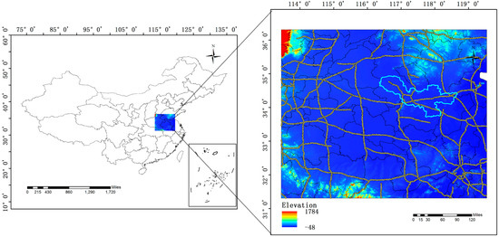
Figure 1.
Borders of China (left); and DEM map of the study area (the highlighted area is the Xuzhou region) (right). The black and yellow lines on the base map represent the administrative boundaries and the highways, respectively.
2.2. Data Used
2.2.1. Meteorological Data
The numerical weather prediction model WRF Version 3.6 was employed to model the meteorological field at hourly time steps with nested domains with resolutions of 27 km, 9 km and 3 km (Figure 2). The boundary values were acquired from the European Centre for Medium-Range Weather Forecasts (ECMWF) reanalysis data (http://www.ecmwf.int) with a resolution of 28 km and a 6-hourly interval. These meteorological outputs were used to force the Lagrangian particle model FLEXPART [28].
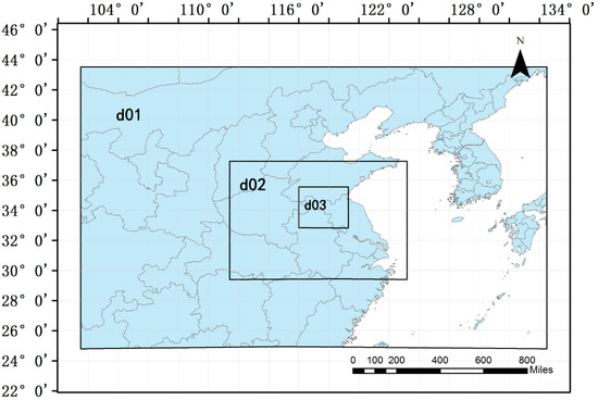
Figure 2.
The nested domains (1–3) used for downscaling.
2.2.2. A Priori PM2.5 Emission Inventory
An a priori air pollutant emission inventory was acquired from the emission inventory of China (i.e., MEIC, http://www.meicmodel.org/), which includes all major anthropogenic emission sources in East Asia at a resolution of 0.25° × 0.25° (Figure 3). Major uncertainties in the PM2.5 emission data in the MEIC inventory were mostly confined to the residential combustion and transportation sectors because their activity data are not well reported through national and provincial statistical systems. The total Xuzhou anthropogenic emissions of PM2.5 in 2010 were estimated to be 3803.5 Mg/month based on the MEIC data.
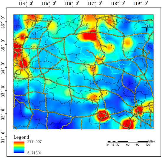
Figure 3.
A priori PM2.5 emission inventory (MEIC). Year: 2010; Flux: Mg/month/0.1 × 0.1°. The black and yellow lines on the base map represent the administrative boundaries and the highways, respectively.
2.2.3. Observations
Figure 4a shows the research area for inversion of the emission inventory. Red dots indicate the locations of observation sites providing hourly PM2.5 concentration data following a quality control assurance procedure that guarantees confidence in the use of these data. To identify and eliminate data outliers, a data quality control algorithm was applied independently to the PM2.5 observations for each observation site. This algorithm has the following components and thresholds [29]:
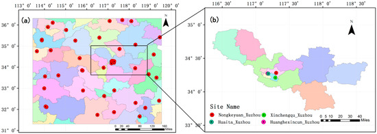
Figure 4.
Research area for inversion of the emission inventory (a); and the research area of Xuzhou containing four sites: Nongkeyuan, Huaita, Huanghexincun and Xinchengqu (b).
- Daily constant value check. If MIN(PM2.5) = MAX(PM2.5) for a 24-h period, then the entire day is eliminated.
- Outliers check. Data over 500 µg/m3 are rejected.
- Single spike. If the difference in PM2.5 concentration between the present hour () and both the previous hour () and the following hour () is greater than 50 , the data for the present hour () are rejected.
- Averaged spike. If the mean concentration over three consecutive hours () is greater than the data in the previous hour () and the following hour () by more than 80 , the data for hours () are rejected.
In addition to the above quality control procedure, a check for frequently missing data at each site was implemented. Following the above tests, approximately 25% of the data were eliminated. An optimizing method was applied to the valid sites that remained, as shown by the red marks in Figure 4b. The research area of Xuzhou contains four sites. For convenience, all the times referenced hereafter are in Beijing Local Time (BLT).
2.3. Model Descriptions
To analyze the corresponding transport of PM2.5 pollution, the coupled FLEXPART-WRF model was employed to calculate forward Lagrangian particle dispersion [5,30,31], driven by the meteorological variables modeled using the WRF model. The FLEXPART-WRF model has been applied and validated for mid-range and long-range transport cases [28,32,33,34]. Compared to an adjoint Eulerian model, the advantage of the LPDM is that no initial diffusion occurs due to the release of the adjoint tracer into a finite-size grid cell, which is independent of a computational grid and has, in principle, infinitesimally small resolution. The Lagrangian model has low computational costs. Furthermore, long-range transport can be simulated more accurately, as no artificial numerical diffusion occurs. In view of the simulation precision of the FLEXPART-WRF system, this system has been previously used for a variety of applications. For example, Srinivas et al. (2014) estimated radiation risk following the 2011 Fukushima nuclear accident using FLEXPART-WRF [35], and the model could reproduce observed deposited activity, albeit with some deviations related to model errors in wind and precipitation data from the WRF model. Gentner et al. (2014) used FLEXPART-WRF in backward mode to determine the source–receptor relationship (SRR) of anthropogenic emissions of organic carbon [36]. Another advantage of FLEXPART-WRF model is that it can obtain the contribution rate of pollutants sources to the receptor points, which makes it possible to improve the accuracy of pollutant forecast using the Bayesian optimization method. However, research on PM2.5 using the FLEXPART model is considerably limited because the current version of FLEXPART-WRF does not support the direct simulation of PM2.5 concentrations. Most studies are based on the off-line coupling of the FLEXPART-WRF model with the WRF-Chem model or the CMAQ model [37]. The emphasis and innovation of this study is to improve the prediction accuracy of PM2.5 by combining the FLEXPART-WRF model with the Bayesian optimization method. Considering the computing time cost and the characteristics of the FLEXPART-WRF model, the experiment design to simulate the pollutant particles as passive tracer air parcels without considering chemical reactions and dry deposition [38]. The chemistry and the dry deposition errors were treated as the errors of pollution sources. In this research, the spatial distribution of the SRR was determined by the Lagrangian particle dispersion model (FLEXPART-WRF). The SRR represents the contribution of each potential source for the receptors (observation sites). The forward simulation was adopted in this experiment, and each emission source had a release rate of 5000 computational particles per hour. Concentrations were sampled on a 3-D output grid every 3 min and used for calculating hourly averages. The trajectories of individual particles were computed using a zero-acceleration scheme, in which particle movements are dependent on the grid-scale wind and the turbulent fluctuations as follows:
Equation (1) is accurate to the first order, and the trajectory equation is integrated as follows [30]:
where t is time, is the time increment, X is the position vector, and is the wind vector, which is composed of grid-scale wind , turbulent wind fluctuations and mesoscale wind fluctuations .
2.4. Inversion Method
2.4.1. Generating the Source–Receptor Relationship
In this study, the source of SRR has different meaning compared to the source stated by Gentner et al. (2014) [36]. In the paper of Gentner et al. (2014), the source indicates petroleum industry and dairy operations, while, in this paper, it refers to the location of the PM2.5 emissions. In the present study, 30-day SRRs were determined by releasing 5000 particles per hour from the potential sources. Here, the potential sources represent the potential locations. Considering the number of emission sources and the lower speed of the serial method, the parallel method is adopted to run the FLEXPART-WRF model. The contaminated area was divided into 30 pieces and run separately and finally, the model results were merged, and the receptor contributions from each pollution source were acquired. To apply the Bayesian optimization method, the potential source locations should be consistent with the grid locations from the MEIC a priori inventory.
In this paper, when simulating the SRR and inverting the PM2.5 inventory, the first two months of the results are not examined because this period corresponds to the typical spin-up period.
2.4.2. Construction Cost Function and Calculation
By combining the Bayesian inversion method and receptor observations, the PM2.5 emission and the corrected real-time PM2.5 were obtained. The principle of inversion is to optimize the emission flux density by minimizing the mismatch between observed and simulated concentrations. The basic equation of the inversion approach can be written as follows:
where M is the matrix of SRR, is a vector of the PM2.5 concentrations (μg/m3) at a receptor, and is the emission flux vector (Mg/grid/month). The equation can be written as follows:
where m is the time series of observations and n is the number of emission grids. is a vector that has m rows. Assuming that and , where , and are the a priori source vector, a posteriori source vector and observation vector, respectively, the cost function is described as follows [39,40]:
The best estimate was obtained by solving the equation as follows:
where and represent the standard errors related to the observations and a priori values, respectively. We are unable to precisely obtain the uncertainty information of each potential source and observation site. Therefore, this study adopted the method from Stohl et al. (2009) to deal with the uncertainty of greenhouse gases [40]. The potential source emission uncertainty is , where and represent the emissions related to the potential source and MEIC average emission flux over the study area, respectively, while observational uncertainty is consisted of the measurement error as well as model errors. Because the model errors are difficult to estimate, the root mean square (RMS) between the observed values and the priori simulated values at each site are used as the uncertainty of observation. Considering that the flux cannot be negative, it needs to have a condition . To reduce unrealistic emissions in the a posteriori inventory, the calculation was iterated until all negative emissions were greater than or equal to 0.
2.4.3. Optimization According to the A Posteriori Inventory for Forecasting PM2.5
Finally, according to the a posteriori inventory, the simulation values were optimized to predict the receptor PM2.5 concentrations.
where t represents the time series of the simulation in the future, which can be understood as the number of hours.
Because of the dramatic changes in the PM2.5 concentrations in response to changes in tropospheric meteorological factors, this paper considers only the contributions from source region-based SRR calculations rather than background values.
2.5. Verification Statistics
The Pearson product-moment coefficient of linear correction is related to the degree of correlation between two fixed distance variables.
The root mean square error (RMSE) is often used to evaluate model performance because it quantifies the magnitude of the error in the model [41,42].
In addition, the index of agreement (IOA) is used in the model evaluation. IOA is defined as follows:
where is the th paired (model-observation) data point, is the total number of paired data points, and and are the th modeled and observed mixing ratios, respectively. and . is the mean observed mixing ratio. IOA specifies the degree to which the observed deviations of correspond, in both magnitude and sign, to the predicted deviations of . The value of IOA varies between 0.0 and 1.0, representing the limits of complete disagreement to perfect agreement between the observations and simulations.
3. Results and Discussion
3.1. Evaluation of the Site Optimizations
For the remainder of the paper, we use observation data for a one-month period in the optimization using the Bayesian optimization schemes. The use of such one-month time series observation data can not only meet the forecast time requirements but also greatly improve the prediction accuracy. Studies have shown that longer simulation times do not result in better reconstruction of emission sources because of the rapid decrease in emission sensitivity and the increase in model error. Table 1 summarizes the statistical measures of the model simulations using a priori and a posteriori emission inventories relative to observations. The correlation coefficient R between the observations and inversion results was , compared with that of using the a prior inventory. The were ~4.039 and ~8.648 µg/m3, respectively. The IOA is another metric that can be used to assess improvements resulting from the application of the Bayesian method, and the IOA increased on average by 21.45%. The Bayesian optimization method adequately removes the systematic mean bias component. The unsystematic component can be reduced significantly through the optimization method. The mean bias of the Bayesian inversion system is 53.2% less than that of the raw results.

Table 1.
Statistical analysis between the a posteriori and a priori inventories.
Figure 5 shows the comparison of the yearly mean diurnal variation of PM2.5 between simulation and observation at four sites in Xuzhou. The simulations with inventory data originating from MEIC (a priori inventory) agree well with the observations. Compared to the observations, the raw model tends to overestimate PM2.5 at night for all four sites. The MEIC inventory data (a priori inventory) are largely skewed towards highly positive PM2.5 errors, with average errors larger than 10–25 µg/m3. In contrast, the optimization results are more consistent with the observation curve. The Bayesian optimization method tends to bring the optimization values closer to the observations than the raw model forecasts. In addition, the results show that, at nighttime and in the early morning, PM2.5 concentrations were higher than at midday because, during the night and early morning, the boundary layer is generally low in height and has weaker convection than during the daytime. However, the simulation deviation is also large using the a priori inventory, which may not have considered the relatively low levels of anthropogenic emissions from factories and motor vehicles in the evening.
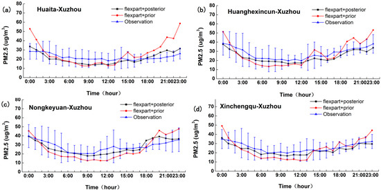
Figure 5.
Comparisons of the yearly mean diurnal variation of simulated PM2.5 in 2016 against observations at the four sites: (a) Huaita-Xuzhou; (b) Huanghexincun-Xuzhou; (c) Nongkeyuan-Xuzhou; and (d) Xinchengqu-Xuzhou. The red line represents the simulation using the a priori inventory, the black line represents the simulation using the a posteriori inventory, and the blue line represents the observations and standard deviation () of the observations. Year: 2016.
The optimization results are not always superior to those of the raw model. For example, the optimization effect of the Huaita-Xuzhou observation site is not as good as the raw model values at 2:00–5:00, although the difference is very small (Figure 5a). This discrepancy may be explained by the fact that the optimization effect is affected not only by the emission inventory but also by the meteorological conditions, the model errors and the pollution emergency event [10,14]. Overall, the results of the Bayesian inversion system in this study are closer to the actual observations, and the inversion emission inventory has greater credibility.
3.2. Evaluation of the Site Forecasts
The forecast values of three days from the a posteriori inventory calculated by the inversion model were compared with observations at four sites in Huaita-Xuzhou, Huanghexincun-Xuzhou, Nongkeyuan-Xuzhou and Xinchengqu-Xuzhou. Application of the Bayesian optimization method produces PM2.5 forecast values that are much closer to the observation values than the raw model. The raw model tends to have larger fluctuations than the observations on almost all days at these stations. As shown in Table 2, the correlation coefficient R between the predicted and observed PM2.5 values was improved using the inversion system, with values of versus after and before using inversion, respectively. Accordingly, the values of were ~7.407 and ~9.805 μg/m3 after and before calibration, respectively. The IOA for the forecasts increased on average by 16.14%. As expected, the optimization method greatly reduced the systematic error, which was an improvement over the raw model forecasts. However, Figure 6 reveals that, while the Bayesian method helped to reduce the systematic errors in the model forecasts, some residual error still exists in the adjusted forecasts. This residual error mainly caused by without considering chemical reactions that are affected by meteorological factors and emissions, and these errors cannot be adequately resolved by the inversion system.

Table 2.
Statistical Analysis Between a Posteriori and a Priori Inventories for Forecasting.
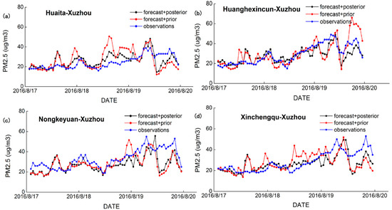
Figure 6.
Comparisons between observations and forecast values of PM2.5 concentrations in the time series for the four sites: (a) Huaita-Xuzhou; (b) Huanghexincun-Xuzhou; (c) Nongkeyuan-Xuzhou; and (d) Xinchengqu-Xuzhou The red line represents the forecast values using the a priori inventory, the black line represents the forecast values using the a posteriori inventory, and the blue line represents the observations. Year: 2016.
Figure 6 shows that the forecast values calculated from the a priori inventory were overestimated to some extent. The forecast values from the a posteriori inventory, by contrast, not only exhibited an improved correlation with observations but also corrected the system error. Comparisons for 17 August, 18 August and 19 August show that the model performed quite well on 17 August and 18 August. However, the model for 19 August did not perform as well as that for 17 and 18August. Previous research has suggested that poor forecast performance with the extension of the forecast time is common among air quality models and may be caused by the difficulty in simulating stagnant weather conditions [43]. This finding may be partially attributed to a combination of effects associated with the current model grid resolution, which is not sufficient to resolve the highly variable meteorological conditions, spatial and temporal variability in emissions, and, consequently, the evolution of the chemistry leading to PM2.5 formation.
Other scholars have used different methods to improve the forecast accuracy of PM2.5. For example, Borrego et al. (2011) evaluated the application of two bias-correction techniques, the multiplicative ratio and the Kalman filter, to improve air quality forecasts [44]. Their statistics showed that both bias-correction techniques improved the raw forecast skills, and the forecasts of PM2.5 improved significantly, with R values ranging from 0.5 to 0.64. The results confirm the advantage of the application of bias-correction techniques for air quality forecasts. However, the Bayesian inversion system, unlike the Kalman filter and multiplicative ratio methods, improves the forecasting accuracy by optimizing the priori inventory rather than merely correcting model forecast values. Therefore, the Bayesian inversion system developed in this study can not only produce better prediction results but also estimate a high-resolution emission inventory.
3.3. Analysis of the Emission Inventory
Figure 7 shows the spatial distribution of the PM2.5 a posteriori emission fluxes in March, June, September and December, representing spring, summer, autumn and winter, respectively. The results show that the emission of PM2.5 was significantly higher in winter than in summer due to fossil fuel combustion for heating. In contrast, the fluxes of MEIC (Figure 3) and the monthly average calculated by the inversion system (Figure 8a) show that the PM2.5 emission flux might be overestimated to some extent by the a priori inventory in the heavy pollution area (Figure 9a), which may be related to the recent prevention and control of pollution. However, a comparison of the a posteriori and INTEX-B emission inventories (Figure 8b), which was conducted by the National Aeronautics and Space Administration (NASA), shows that the a posteriori PM2.5 emissions are generally higher than the INTEX-B emission flux (Figure 9b). One of the possible reasons for this finding is that the INTEX-B emission inventory has a low spatial resolution and time lag. Overall, the spatial features of the a posteriori values were generally consistent with the latest regional emission inventory in the study areas.
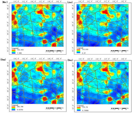
Figure 7.
PM2.5 emission flux per month. Year: 2016; Flux: Mg/month/0.1 × 0.1°. The black and yellow lines on the base map represent the administrative boundaries and the highways, respectively.
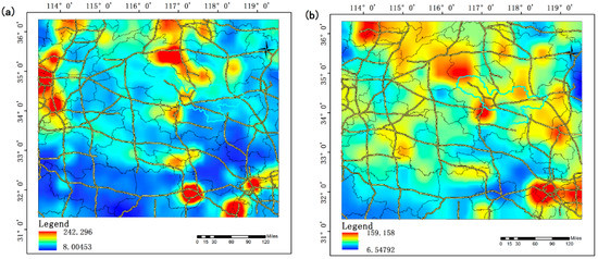
Figure 8.
PM2.5 emission flux (Mg/month/0.1 × 0.1°): (a) monthly average PM2.5 emission flux (Year: 2016); and (b) INTEX-B emission flux (Year: 2006). The black and yellow lines on the base map represent the administrative boundaries and the highways, respectively.
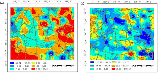
Figure 9.
Difference between emission flux values (Mg/month/0.1 × 0.1°): (a) difference between the a posteriori and a priori emission flux values; and (b) difference between the a posteriori and INTEX-B emission flux values. The black and yellow lines on the base map represent the administrative boundaries and the highways, respectively.
A comparison of PM2.5 emissions at a city level between a priori and a posteriori values is shown in Table 3 and Figure 10 (the a posteriori inventory and MEIC statistical values). Table 3 shows the adjustment for the a posteriori values (difference between a posteriori and a priori) for Xuzhou, Suqian, Hefei and Jining, where the inversion results were statistically 384.76 Mg/month and 451.50 Mg/month larger than the a priori values in Xuzhou and Suqian, respectively. The statistics showed that the a posteriori PM2.5 emissions increase by 10.12% and 27.84% for Xuzhou and Suqian, respectively. However, the inversion results were smaller than the a priori values in Hefei and Jining by 561.41 Mg/month and 634.32 Mg/month, respectively, which showed that the a posteriori emissions decreased by 10.83% and 9.58%, respectively. The differences between a priori and posteriori can stem from three reasons: the errors of inversion system, a priori inventory errors and the effect of time lag. The a priori inventory was from the MEIC data of 2010, but the study period was 2016. The impact of time lag mainly refers to the changes in pollutant emissions caused by the rapid development of china’s economy [45]. During this period, the rapid growth of urbanization and rising consumption of fossil fuels increased the emissions of pollutant, while the implementation of industrial energy saving and emission reduction measures also reduced the emissions of pollutant in the meantime.

Table 3.
Difference between a posteriori and a priori values.
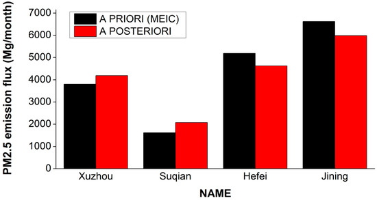
Figure 10.
Statistical results of PM2.5 emission flux for a priori and a posteriori values in Xuzhou, Suqian, Hefei and Jining.
Figure 11 shows the trends of monthly PM2.5 for the cities of Xuzhou, Jining, Hefei, and Suqian in 2016. The PM2.5 emission is lower in the summer and higher in the winter because abundant heating fuel is needed in the winter, which produces many fine particulates in the atmosphere. However, the PM2.5 emissions increase to some extent due to the large-scale burning of crops straw in the summer harvesting season. The obvious deviations of the PM2.5 emission flux at certain locations in the diagram could be partly attributed to the failure to account for chemical transformation, and the corresponding SRR might exclude the emission signal associated with open biomass burning sources.
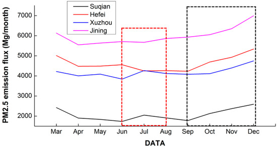
Figure 11.
Trends in the PM2.5 emission flux per month for the cities of Xuzhou, Hefei, Jining and Suqian. Year: 2016. The red and black dashed lines represent the period in summer and winter, respectively.
4. Conclusions
In this study, the emission inventory and real-time PM2.5 concentration in Xuzhou are inverted by the Bayesian optimization method based on tower observations. The general feature of the inversion results is that the a posteriori values are consistent with the latest MEIC emission inventory, and the prediction accuracy is greatly improved. The R and values between the observations and the forecast values were improved by approximately 39.2% and 24.5%, respectively, using the inversion system. However, the present results imply that the PM2.5 emissions in the Xuzhou region might be significantly underestimated by bottom-up statistical methods. In general, the present PM2.5 emission inventory inversion implies a 10.12% increase between 2010 and 2016 in Xuzhou. Although our analysis suggests that the Bayesian method can significantly reduce the systematic errors, the relative improvements of the real-time PM2.5 forecast values from the application of this method were limited in terms of the temporal extent of the forecast. The inversion approaches still have considerable uncertainties due to the limited observation sites and the method limitations. Our future work will involve an assessment of inversion accuracy by including multiple sites in Xuzhou, and the seasonal variation will be addressed using a long-term observation dataset. At present, this study only verified the posteriori inventory is better than the a priori inventory for improving the forecast accuracy of PM2.5. We also need to combine the models of WRF-Chem and CMAQ for further verification.
In the applications presented in this study, the Bayesian optimization method is applied only at discrete points of the monitors. The extension of these methods for the development of optimized spatial map forecasting surface-level PM2.5 distributions is an area for further research.
Author Contributions
Conceptualization, B.C. and L.G.; Methodology, L.G.; Software, L.G.; Validation, G.X., L.L. and Y.L.; Formal Analysis, L.G.; Investigation, L.G.; Resources, B.C.; Data Curation, L.G., X.L. and F.W.; Writing-Original Draft Preparation, L.G.; Writing-Review & Editing, B.C. and H.Z.; Visualization, L.G. and Y.K.; Supervision, B.C.; Project Administration, B.C.; Funding Acquisition, B.C.
Funding
This research was funded by the international partnership program of Chinese Academy of Sciences (Grant #131A11KYSB20170025) and research grants funded by the State Key Laboratory of Resources and Environment Information System (O88RA901YA) and funded by the National Natural Science Foundation of China (41771114).
Acknowledgments
We thank Qiang Zhang’s team from the Tsinghua University for providing the multiscale emission inventory of China’s (MEIC) data.
Conflicts of Interest
The authors declare no conflict of interest. The funders had no role in the design of the study; in the collection, analyses, or interpretation of data; in the writing of the manuscript; or in the decision to publish the results.
References
- Zhao, X.; Shi, H.; Yu, H.; Yang, P. Inversion of Nighttime PM2.5 Mass Concentration in Beijing Based on the VIIRS Day-Night Band. Atmosphere 2016, 7, 136. [Google Scholar] [CrossRef]
- Yang, F.M.; Ma, Y.L.; He, K.B. A brief introduction to PM2.5 and related research. World Environ. 2000, 2000, 32–34. [Google Scholar]
- Zhang, Q.; Quan, J.; Tie, X.; Li, X.; Liu, Q.; Gao, Y.; Zhao, D. Effects of meteorology and secondary particle formation on visibility during heavy haze events in Beijing, China. Sci. Total Environ. 2015, 502, 578–584. [Google Scholar] [CrossRef] [PubMed]
- Yang, Y.; Liu, X.; Qu, Y.; Wang, J.; An, J.; Zhang, Y.; Zhang, F. Formation mechanism of continuous extreme haze episodes in the megacity Beijing, China, in January 2013. Atmos. Res. 2015, 155, 192–203. [Google Scholar] [CrossRef]
- Bei, N.; Xiao, B.; Meng, N.; Feng, T. Critical role of meteorological conditions in a persistent haze episode in the Guanzhong basin, China. Sci. Total Environ. 2016, 550, 273–284. [Google Scholar] [CrossRef] [PubMed]
- Cuvelier, C.; Thunis, P.; Vautard, R.; Amann, M.; Bessagnet, B.; Bedogni, M.; Berkowicz, R.; Brandt, J.; Brocheton, F.; Builtjes, P.; et al. CityDelta: A model intercomparison study to explore the impact of emission reductions in European cities in 2010. Atmos. Environ. 2007, 41, 189–207. [Google Scholar] [CrossRef]
- EPA. Guidelines for Developing an Air Quality Forecasting Program; Environmental Protection Agency Report, EPA-456/R-03-002; Environmental Protection Agency: Washington, DC, USA, 2003.
- Dong, M.; Yang, D.; Kuang, Y.; He, D.; Erdal, S.; Kenski, D. PM2.5, concentration prediction using hidden semi-Markov model-based times series data mining. Expert Syst. Appl. 2009, 36, 9046–9055. [Google Scholar] [CrossRef]
- Baklanov, A. Overview of the European project FUMAPEX. Atmos. Chem. Phys. Discuss. 2005, 5, 2005–2015. [Google Scholar] [CrossRef]
- Fay, B.; Userer, L.N. Evaluation of high-resolution forecasts with the non-hydrostaticnumerical weather prediction model Lokalmodell for urban air pollutionepisodes in Helsinki, Oslo and Valencia. Atmos. Chem. Phys. 2006, 6, 2107–2128. [Google Scholar] [CrossRef]
- Palau, J.L.; Pérezlanda, G.; Diéguez, J.J.; Monter, C.; Millán, M.M. The importance of meteorological scales to forecast air pollution scenarios on coastal complex terrain. Atmos. Chem. Phys. 2005, 5, 2771–2785. [Google Scholar] [CrossRef]
- Schroeder, A.J.; Stauffer, D.R.; Seaman, N.L.; Deng, A.; Gibbs, A.M.; Hunter, G.K.; Young, G.S. An Automated High-Resolution, Rapidly Relocatable Meteorological Nowcasting and Prediction System. Mon. Weather Rev. 2006, 134, 1237–1265. [Google Scholar] [CrossRef]
- Finardi, S.; Maria, R.D.; D’Allura, A.; Cascone, C.; Calori, G.; Lollobrigida, F. A deterministic air quality forecasting system for Torino urban area, Italy. Environ. Model. Softw. 2008, 23, 344–355. [Google Scholar] [CrossRef]
- Baklanov, A.; Mestayer, P.G.; Clappier, A.; Zilitinkevich, S.; Joffre, S.; Mahura, A.; Nielsen, N.W. Towards improving the simulation of meteorological fields in urban areas through updated/advanced surface fluxes description. Atmos. Chem. Phys. 2008, 8, 523–543. [Google Scholar] [CrossRef]
- Borrego, C.; Schatzmann, M.; Galmarini, S. Quality Assurance of Air Pollution Models. In Air Quality in Cities; Springer: Berlin/Heidelberg, Germany, 2003; pp. 155–183. [Google Scholar]
- Borrego, C.; Monteiro, A.; Ferreira, J.; Miranda, A.I.; Costa, A.M.; Carvalho, A.C.; Lopes, M. Procedures for estimation of modelling uncertainty in air quality assessment. Environ. Int. 2008, 34, 613–620. [Google Scholar] [CrossRef] [PubMed]
- Chang, J.C.; Hanna, S.R. Air quality model performance evaluation. Meteorol. Atmos. Phys. 2004, 87, 167–196. [Google Scholar] [CrossRef]
- Mckeen, S.; Wilczak, J.; Grell, G.; Djalalova, I.; Peckham, S.; Hsie, E.-Y.; Gong, W.; Bouchet, V.; Menard, S.; Moffet, R.; et al. Assessment of an ensemble of seven real-time ozone forecasts over eastern North America during the summer of 2004. J. Geophys. Res. 2005, 110, 3003–3013. [Google Scholar] [CrossRef]
- Pagowski, M.; Grell, G.A.; Devenyi, D.; Peckham, S.E.; McKeen, S.A.; Gong, W.; Monache, L.D.; McHenry, J.N.; McQueen, J.; Lee, P. Application of dynamic linear regression to improve the skill of ensemble-based deterministic ozone forecasts. Atmos. Environ. 2006, 40, 3240–3250. [Google Scholar] [CrossRef]
- Djalalova, I.; Wilczak, J.; Mckeen, S.; Grell, G.; Peckham, S.; Pagowski, M.; DelleMonache, L.; McQueen, J.; Tang, Y.; Lee, P.; et al. Ensemble and bias-correction techniques for air quality model forecasts of surface O3, and PM2.5, during the TEXAQS-II experiment of 2006. Atmos. Environ. 2010, 44, 455–467. [Google Scholar] [CrossRef]
- Sicardi, V.; Ortiz, J.; Rincón, A.; Jorba Casellas, O.; Pay Pérez, M.T.; Gassó Domingo, S.; Baldasano Recio, J.M. Ground-level ozone concentration over Spain: An application of Kalman Filter post-processing to reduce model uncertainties. Geosci. Model Dev. Discuss. 2011, 4, 343–384. [Google Scholar] [CrossRef]
- Abderrahim, H.; Chellali, M.R.; Hamou, A. Forecasting PM10, in Algiers: Efficacy of multilayer perceptron networks. Environ. Sci. Pollut. Res. Int. 2016, 23, 1634–1641. [Google Scholar] [CrossRef] [PubMed]
- Biancofiore, F.; Busilacchio, M.; Verdecchia, M.; Tomassetti, B.; Aruffo, E.; Bianco, S.; Di Tommaso, S.; Colangeli, C.; Rosatelli, G.; Di Carlo, P. Recursive neural network model for analysis and forecast of PM10 and PM2.5. Atmos. Pollut. Res. 2017, 8, 652–659. [Google Scholar] [CrossRef]
- Monache, L.D.; Nipen, T.; Deng, X.; Zhou, Y.; Stull, R. Ozone ensemble forecasts: 2. A Kalman filter predictor bias correction. J. Geophys. Res. Atmos. 2006, 111. [Google Scholar] [CrossRef]
- Kang, D.; Mathur, R.; Rao, S.T.; Yu, S. Bias adjustment techniques for improving ozone air quality forecasts. J. Geophys. Res. Atmos. 2008, 113. [Google Scholar] [CrossRef]
- Zhang, Q.; Streets, D.G.; Carmichael, G.R.; He, K.B.; Huo, H.; Kannari, A.; Klimont, Z.; Park, I.S.; Reddy, S.; Fu, J.S.; et al. Asian emissions in 2006 for the NASA INTEX-B mission. Atmos. Chem. Phys. 2009, 9, 5131–5153. [Google Scholar] [CrossRef]
- Li, Q.; Jiang, J.; Wang, S.; Rumchev, K.; Mead-Hunter, R.; Morawska, L.; Hao, J. Impacts of household coal and biomass combustion on indoor and ambient air quality in China: Current status and implication. Sci. Total Environ. 2017, 576, 347–361. [Google Scholar] [CrossRef] [PubMed]
- Brioude, J.; Arnold, D.; Stohl, A.; Cassiani, M.; Morton, D.; Seibert, P.; Angevine, W.; Evan, S.; Dingwell, A.; Fast, J.D.; et al. The Lagrangian particle dispersion model FLEXPART-WRF version 3.0. Geosci. Model Dev. Discuss. 2013, 6, 1889–1904. [Google Scholar] [CrossRef]
- Djalalova, I.; Monache, L.D.; Wilczak, J. PM2.5, analog forecast and Kalman filter post-processing for the Community Multiscale Air Quality (CMAQ) model. Atmos. Environ. 2015, 119, 431–442. [Google Scholar] [CrossRef]
- Stohl, A.; Hittenberger, M.; Wotawa, G. Validation of the Lagrangian particle dispersion model FLEXPART against largescale tracer experiment data. Atmos. Environ. 1998, 32, 4245–4264. [Google Scholar] [CrossRef]
- Fast, J.D.; Easter, R.C. A Lagrangian particle dispersion model compatible with WRF. In Proceedings of the 7th Annual WRF User’s Workshop, Boulder, CO, USA, 19–22 June 2006; pp. 19–22. [Google Scholar]
- Angevine, W.M.; Brioude, J.; McKeen, S.; Holloway, J.S.; Lerner, B.M.; Goldstein, A.H.; Guha, A.; Andrews, A.; Nowak, J.B.; Evan, S.; et al. Pollutant transport among California regions. J. Geophys. Res. Atmos. 2013, 118, 6750–6763. [Google Scholar] [CrossRef]
- Madala, S.; Satyanarayana, A.N.V.; Srinivas, C.V.; Kumar, M. Mesoscale atmospheric flowfield simulations for air quality modeling over complex terrain region of Ranchi in eastern India using WRF. Atmos. Environ. 2015, 107, 315–328. [Google Scholar] [CrossRef]
- Cécé, R.; Bernard, D.; Brioude, J.; Zahibo, N. Microscale anthropogenic pollution modelling in a small tropical island during weak trade winds: Lagrangian particle dispersion simulations using real nested LES meteorological fields. Atmos. Environ. 2016, 139, 98–112. [Google Scholar] [CrossRef]
- Srinivas, C.V.; Rakesh, P.T.; Prasad, K.H.; Venkatesan, R.; Baskaran, R.; Venkatraman, B. Assessment of atmospheric dispersion and radiological impact from the Fukushima accident in a 40 km range using a simulation approach. Air Qual. Atmos. Health 2014, 7, 209–227. [Google Scholar] [CrossRef]
- Gentner, D.R.; Ford, T.B.; Guha, A.; Boulanger, K.; Brioude, J.; Angevine, W.M.; de Gouw, J.A.; Warneke, C.; Gilman, J.B.; Ryerson, T.B.; et al. Emissions of organic carbon and methane from petroleum and dairy operations in California’s San Joaquin Valley. Atmos. Chem. Phys. 2014, 14, 4955–4978. [Google Scholar] [CrossRef]
- Marelle, L.; Raut, J.C.; Thomas, J.L.; Law, K.S.; Quennehen, B.; Ancellet, G.; Pelon, G.; Schwarzenboeck, A.; Fast, J.D. Transport of anthropogenic and biomass burning aerosols from Europe to the Arctic during spring 2008. Atmos. Chem. Phys. 2015, 15, 3831–3850. [Google Scholar] [CrossRef]
- Li, W.J.; Chen, S.R.; Xu, Y.S.; Guo, X.C.; Sun, Y.L.; Yang, X.Y.; Wang, Z.F.; Zhao, X.D.; Chen, J.M.; Wang, W.X. Mixing state and sources of submicron regional background aerosols in the northern Qinghai-Tibet Plateau and the influence of biomass burning. Atmos. Chem. Phys. 2015, 15, 13365–13376. [Google Scholar] [CrossRef]
- Pan, X.L.; Kanaya, Y.; Wang, Z.F.; Tang, X.; Takigawa, M.; Pakpong, P.; Taketani, F.; Akimoto, H. Using Bayesian optimization method and FLEXPART tracer model to evaluate CO emission in East China in springtime. Environ. Sci. Pollut. Res. Int. 2014, 21, 3873–3879. [Google Scholar] [CrossRef] [PubMed]
- Stohl, A.; Seibert, P.; Arduini, J.; Eckhardt, S.; Fraser, P.; Greally, B.R.; Maione, M.; O’Doherty, S.; Prinn, R.G.; Reimann, S.; et al. A new analytical inversion method for determining regional and global emissions of greenhouse gases: Sensitivity studies and application to halocarbons. Atmos. Chem. Phys. 2009, 69, 1026–1027. [Google Scholar] [CrossRef]
- Willmott, C.J.; Ackleson, S.G.; Davis, R.E.; Feddema, J.J.; Klink, K.M.; Legates, D.R.; O’Donnell, J.; Rowe, C.M. Statistics for the evaluation and comparison of models. J. Geophys. Res. Oceans 1985, 90, 8995–9005. [Google Scholar] [CrossRef]
- Willmott, C.J.; Matsuura, K. Advantages of the Mean Absolute Error (MAE) over the Root Mean Square Error (RMSE) in Assessing Average Model Performance. Clim. Res. 2005, 30, 79–82. [Google Scholar] [CrossRef]
- Lyu, B.; Zhang, Y.; Hu, Y. Improving PM2.5 Air Quality Model Forecasts in China Using a Bias-Correction Framework. Atmosphere 2017, 8, 147. [Google Scholar] [CrossRef]
- Borrego, C.; Monteiro, A.; Pay, M.T.; Ribeiro, I.; Miranda, A.I.; Basart, S.; Baldasano, J.M. How bias-correction can improve air quality forecasts over Portugal. Atmos. Environ. 2011, 45, 6629–6641. [Google Scholar] [CrossRef]
- Wang, H.J.; Chen, H.P. Understanding the recent trend of haze pollution in eastern China: Roles of climate change. Atmos. Chem. Phys. 2016, 16, 1–18. [Google Scholar] [CrossRef]
© 2018 by the authors. Licensee MDPI, Basel, Switzerland. This article is an open access article distributed under the terms and conditions of the Creative Commons Attribution (CC BY) license (http://creativecommons.org/licenses/by/4.0/).