Re-Examination of the Decadal Change in the Relationship between the East Asian Summer Monsoon and Indian Ocean SST

Abstract

This study examines the decadal change in the relationship between two major Indian Ocean (IO) sea surface temperature patterns, namely the Indian Ocean dipole (IOD) and northern IO and the East Asia summer monsoon (EASM) in the early 2000s. In 1991–1999, the former epoch, the interannual variability of EASM was associated with the IOD-like pattern in the original paper and its relationship weakened in 2000–2016. There are two possible causes for this decadal change; stronger land-sea thermal contrast as a local forcing in latter epoch, which may result in the weakening of the relationship between the IO and the EASM. In addition, the influence of El Niño-southern Oscillation (ENSO) on the western North Pacific subtropical high (WNPSH) could be changed depending on the frequency of ENSO. In the 2000s, the intensity of the low frequency (LF)-type ENSO (42–86 months period) events was weaker compared to the former epoch but that of quasi-biennial (QB)-type ENSO (16–36 months period) remained persistent. This could explain that the QB-type ENSO is remote forcing that modulates the change in the relationship between the tropical IO patterns and EASM in the 2000s.

1. Introduction

The Asian summer monsoon includes three monsoon subsystems, namely the East Asian summer monsoon (EASM), western North Pacific summer monsoon (WNPSM) and the Indian summer monsoon (ISM) [1,2]. Because the EASM is located at the midlatitudes and is affected by the tropics and the mid latitude system, EASM is has a fairly complex structure [3]. In addition, the associated monsoon circulation in summer induces various disasters such as flood, drought and landslide, which lead to serious environmental, economic and social losses and human casualties. Thus, prediction of the EASM for the next decade is necessary to prevent a large amount of losses in various fields and it should be more emphasized [4,5].

The EASM has multi-timescale variabilities such as intraseasonal, interannual, decadal and interdecadal variability [2,6,7]. Interannual variation in the anomalous heating over Tibetan Plateau (TP) has an effect on the interannual variation in the EASM and enhances the rainfall over East Asia. The mechanisms of connection induced by the TP warming are the isentropic uplift to the east of the TP and the Rossby wave teleconnection pattern. The remote impact of Rossby wave starts from the upper-level troposphere, propagating eastward and downward and dispersion of the wave generates upper-level anticyclonic circulation with a strong northerly to its east side and a weak southerly to its west side. Thus, cyclonic vorticity develops to the east of the strong northerly and then the wave train develops along the westerly Jet stream at around 40° N. Then, the downward motion results in the low-level anticyclone to the east of Japan [8]. Additionally, the interannual variability of the EASM is related to the El Niño-Southern Oscillation (ENSO) during its developing and decaying phase and there is a bridge structure linking to the EASM and ENSO via the anomalous western North Pacific Subtropical High (WNPSH) [9,10]. In particular, in the Yangtze River Valley, the excessive rainfall is affected by El Niño events during its decaying phase [11,12]. Other relationships between the interannual variability of EASM and the Eurasian winter/spring snow cover [13], Indian Ocean (IO) sea surface temperature anomalies (SSTA) [14], Pacific SSTA patterns [15,16,17,18], Northern Atlantic Oscillation (NAO) and Arctic Oscillation (AO) [19,20] have been investigated in previous studies.

The interdecadal relationship shifts between East Asian summer monsoon index (EASMI) and other phenomena were observed in the late-1970s in many previous studies [21,22,23,24]. Studied by Ding et al. (2010) [21] showed the interdecadal change in the relationship between EASM and the tropical IO for 1953–1975 and 1979–2000 and the distinct SSTA patterns over the tropical IO were associated with the EASMI during each period. The causes of interdecadal shift in the relationship were weakened land-sea thermal contrast and interaction between the ENSO and IO. After 2000, the EASM circulation shows a decadal shift, which is completely different from patterns in previous periods [25]. In accordance with Huang et al. (2018) [25], for 1979–1999, the western Pacific subtropical high (WPSH) show significant influence on the EASM. Meanwhile, after 2000, the Pacific-Japan (PJ) pattern has been absent and the influence of WPSH on the EASM has become weaker. As the part of WPSH region is included in the region used in this study to define EASMI, we focus on the interannual and decadal variability of EASMI. Besides, we have observed the decadal shift in the relationship with the tropical IO which is an important external forcing of the EASM. Since it is important to prepare for disasters in near future (within 10-year) such as flood, drought associated with the tropical IO SST pattern, observing the decadal shift in the relationship is meaningful. In this study, we examine the decadal change in the relationship between the tropical IO SSTA patterns and EASM for 1991–2016 and suggest possible factors that can contribute to the change in relationship between the tropical IO-EASM.

This paper is organized as follows: Section 2 explains the dataset and analysis methods used in this study. In Section 3, we quantify the decadal changes in EASM related to the SSTA patterns in the tropical IO and analyze anomalous atmospheric circulation pattern responses by EASMI and tropical IO indices to compare their interannual variability with decadal changes in the relationship. In Section 4, the possible reasons for the change in relationship between EASMI and tropical IO are discussed. The discussion and conclusion are provided in Section 5.

2. Data and Methodology

The monthly mean datasets used in this study are circulation variables from National Centers for Environmental Prediction (NCEP)/National Center for Atmospheric Research (NCAR) reanalysis dataset, the European Centre for Medium-Range Weather Forecast (ECMWF) Interim reanalysis dataset and the Sea surface temperature (SST) field from the National Oceanic and Atmospheric Administration (NOAA) Extended Reconstructed SST (ERSST) version 5 and precipitation field from the Global Precipitation Climatology Project (GPCP) (

Table 1. Datasets used in this study.

Data	NCEP/NCAR	ERA-interim	GPCP	ERSST
Variables	UV 850 hPa, Z 500 hPa	2 m T	Precipitation	SST
Analysis Period	1953–2016	1979–2016	1979–2016	1953–2016

). The atmospheric variables from the NCEP/NCAR reanalysis are the geopotential height at 500 hPa, zonal and meridional wind at 850 hPa and the surface air temperature is from ERA-interim.

To characterize the interannual variability and seasonal cycle of the East Asian monsoon, the EASMI is defined by the regionally averaged seasonal (JJA) dynamical normalized seasonality (DNS) over the East Asian monsoon domain (10° N–40° N, 110° E–140° E) [26]. The DNS is derived from

$$\delta = \frac{\Vert \overline{V_1}-V_i\Vert }{\Vert \overline{V}\Vert }-2,$$

(1)

where $\overline{V_1}$ and $V_i$ are the January climatology and monthly wind vectors at 850 hPa on each grid point, respectively and $\overline{V}$ is the mean of the January and July climatological wind vector at the same grid point. The value 2 is subtracted on the right side of Equation (1) because 2 is the critical value of significance for the quantity $\frac{\Vert \overline{V_1}-V_i\Vert }{\Vert \overline{V}\Vert }$ [26]. The positive $\delta$ denotes the summer monsoon and the negative $\delta$ denotes the winter monsoon in the Northern Hemisphere. It should be noted that the definition of the EASMI is controversial [27]. The EASMI used here emphasizes the northern China rainfall and has a different meaning to the conventional WNPSM index. A positive value of the EASMI is characterized by an extensive southerly penetrating inland to northern China, which corresponds to enhanced rainfall in northern China and a weak mei-yu/baiu/changma. Despite the reversed sign of the EASMI, our results obtained in this study remain robust.

In the leading EOF modes of the tropical IO SSTA in 1953–2016, the first mode is the Indian Ocean Basin (IOB) mode, which includes the Northern Indian Ocean (NIO) mode and the second is the Indian Ocean Dipole (IOD) mode [28]. The Indian Ocean Dipole index (IODI) is defined by a time series, which represents the difference in area averaged SSTA between the tropical western IO (10° S–10° N, 50° E–70° E) and the tropical eastern IO (10° S–10° N, 90° E–110° E) [28]. As the positive IOD mode is described, the warming (cooling) pattern is in the tropical western IO (eastern IO). In addition, the northern Indian Ocean index (NIOI) is defined by area averaged SSTA over the northern IO (5° S–25° N, 50° E–100° E) [21]. We examine the NIO mode instead of the IOB mode to illustrate the complexity of the tropical IO warming. The tropical Indian Ocean exhibits warming trend almost all the year round and shows considerable regional variations. The SST patterns over the NIO show differences depending on the season and the latent heat flux over the NIO shows two peaks in Nov–Dec and Jun–Aug, with the summer peak showing a larger magnitude. Besides, in the summer, the monsoon westerlies are located in the NIO and move into the western North Pacific (WNP) region via the South China Sea [29]. Therefore, NIO is more suitable than IOB for exploring the relationship between EASM and tropical IO.

We have used the original indices (e.g., EASMI, IODI, NIOI, NAO, ENSO indices) without any filtering to calculate the relationship. For the analysis, we have removed the annual cycle and applied 11 year high-pass filter from circulation variables to explore the relationship between interannual variabilities of circulation anomalies during each period, which is similar to removing the low-frequency variability or a trend for the period. The high pass filter effectively eliminates all variability at time scales longer than the cutoff and achieves a robust interannual signal. Following Ding et al. (2010) [21], we carried out the 15-year sliding correlation computation for the year −7 to year +7 period with additional datasets after 2000. The sliding correlation method is used to quantitatively examine the decadal change in relationship between the EASM and other phenomena. Ding et al. (2010) [21] separated the entire period (1953–2000) into two parts: PRE (1953–1975) and POST (1979–2000). However, in this study, the whole period (1953–2016) is longer than that of datasets used in Ding et al. (2010) [21] and is separated into four parts with distinct correlation patterns between EASM and tropical IO. These four parts are defined as follows: P1 (1953–1975), P2 (1979–1990), P3 (1991–1999) and P4 (2000–2016). Therefore, the POST part (1979–2000) defined in Ding et al. (2010) [21] is divided into two periods (P2 and P3) in this study.

3. Decadal Change in the Relationship between the Tropical IO-East Asian Summer Monsoon

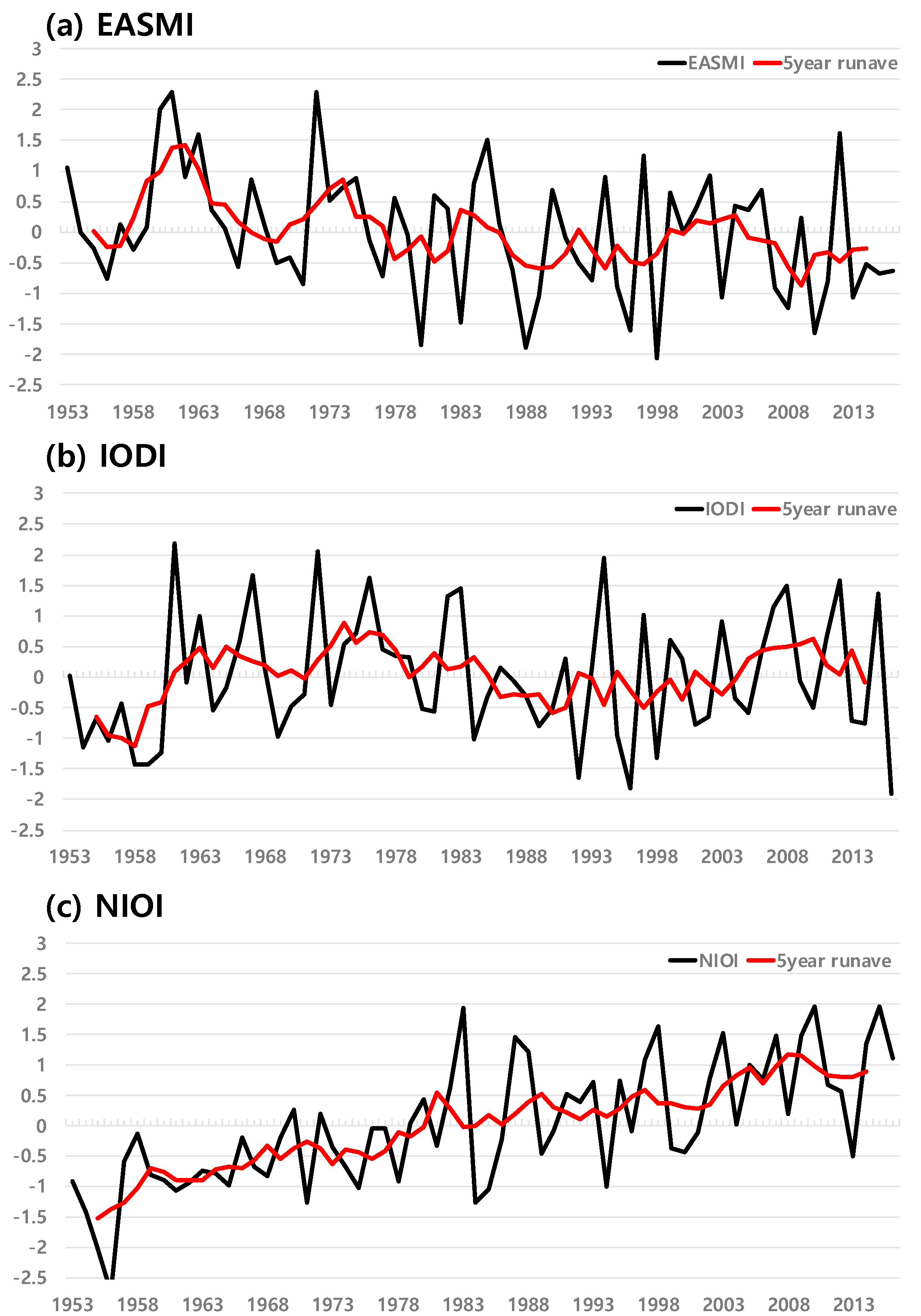
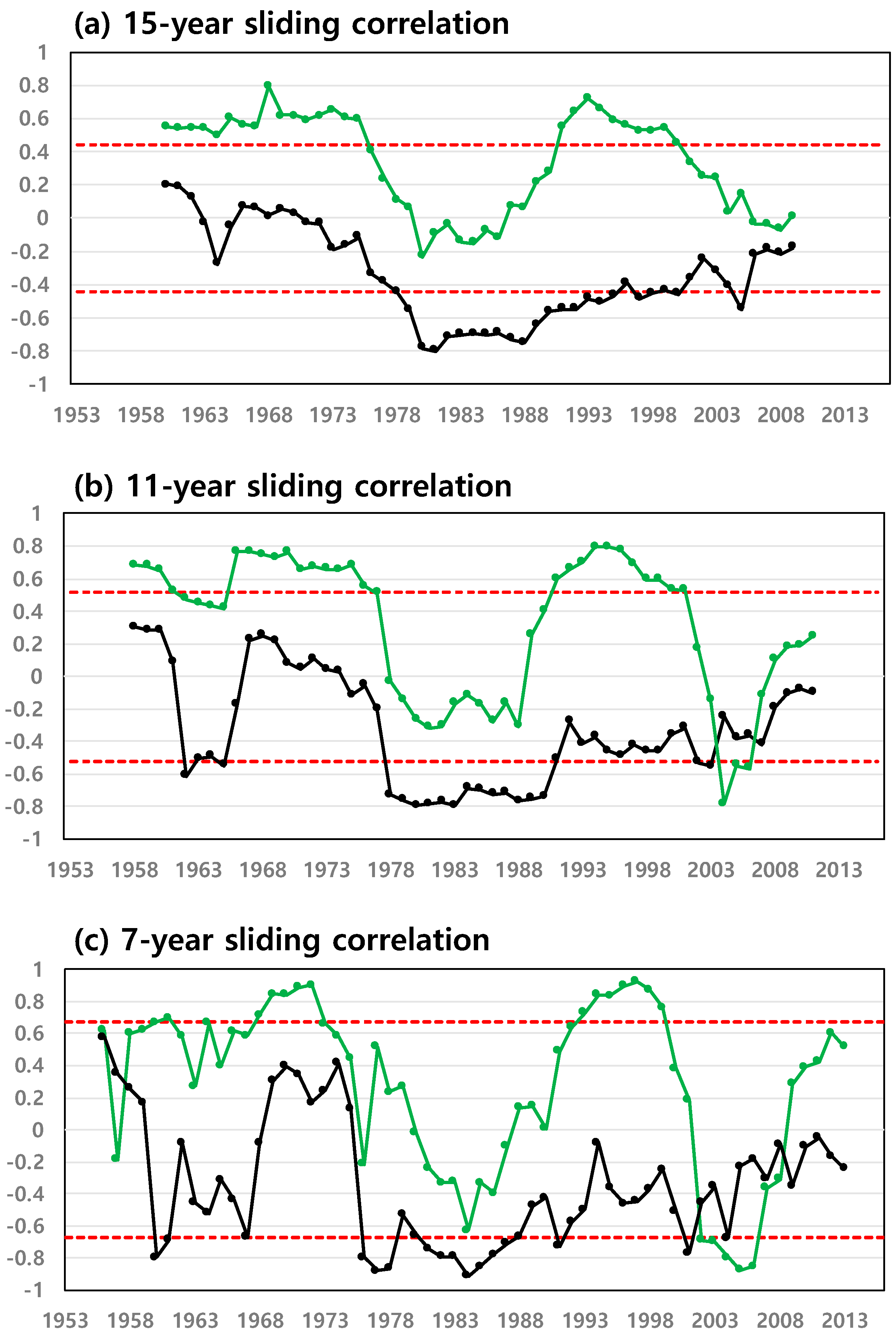
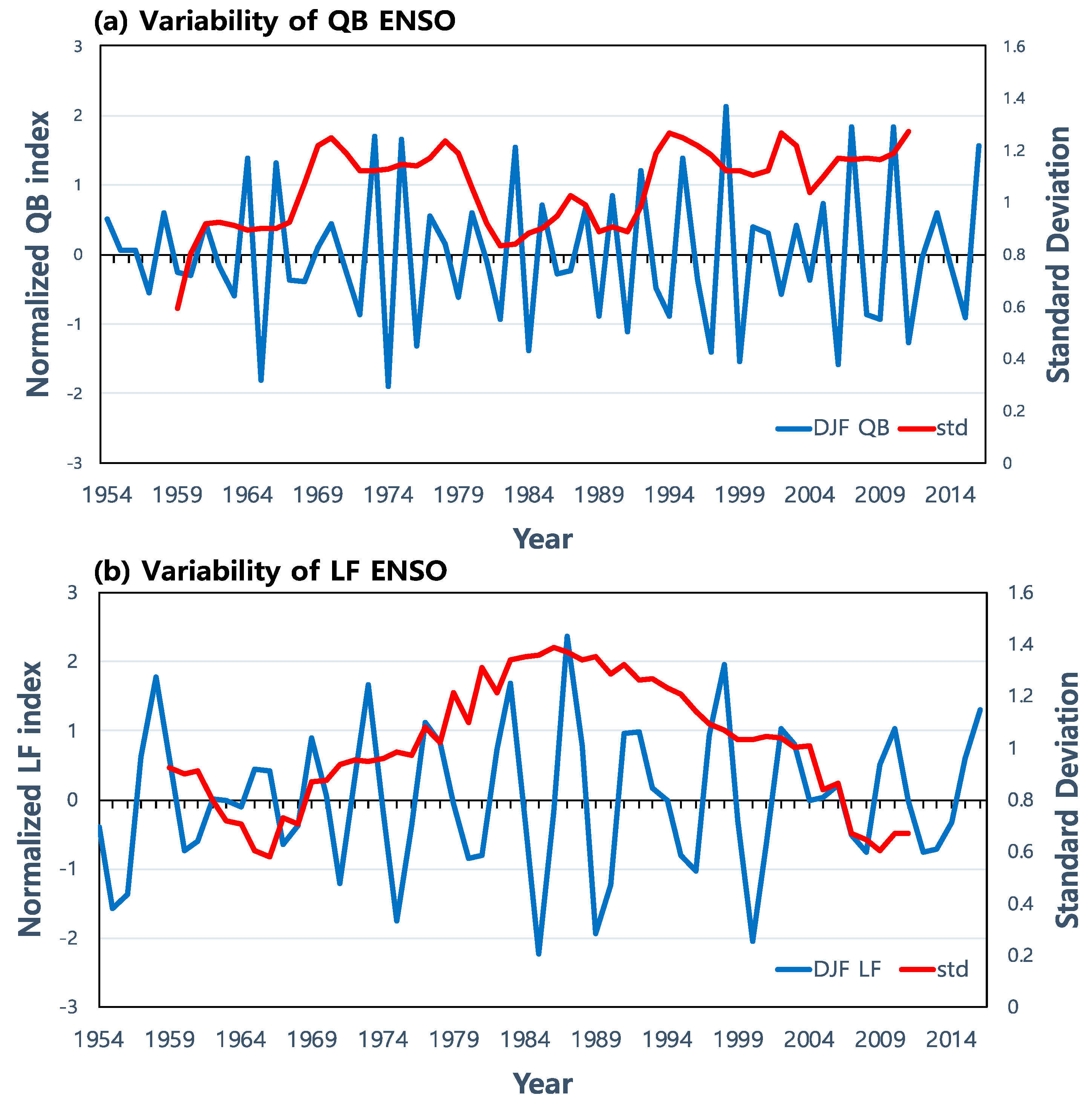
3.1. Examining the Revisited Relationship between the Tropical IO-EASM

To determine the characteristics of the indices, Figure 1 shows normalized interannual variability of EASMI, IODI and NIOI with decadal variability superposed upon it. All indices have explicit interannual variability. The EASMI also has dominant decadal variability and slightly negative trend with weakened intensity after late 1970s. In accordance with Li and Zeng (2002) [26], there is clear connection between the EASMI and summer rainfall in the lower-middle reaches of the Yangtze River in China. In particular, droughts appearing in the valley are associated with strong positive EASMI years. Moreover, summer precipitation in the East Asia clearly displays a PJ pattern with wet WNP region and dried EASM region in strong positive EASMI years. The IODI has weak decadal variation and is expected to get relatively strong interdecadal variation. In the NIOI, it has weak decadal variation and positive trend associated with the global warming [30].

Based on the 15-year sliding correlation patterns, the whole period (1953–2016) is divided into four parts with distinct relationships between the tropical IO-EASMI (Figure 2a). When the individual time series of sliding correlation are computed with a 15-year sliding window (Figure 2a), the endpoints of the decided period boundaries are not close to the actual values because the sliding correlation method was used. However, in the other sliding correlations with shorter sliding window lengths (Figure 2b,c), the endpoints are very close to the result determined by 15-year sliding window. Therefore, the decided endpoints are meaningful. In the first period (1953–1975), the EASMI is highly related to positive IODI (Figure 2), which indicates that a positive correlation pattern exists in the western IO and a negative correlation pattern exists in the eastern IO (Figure 3a). In the second period (1979–1990), the EASMI is significantly related to the negative NIO, not to the positive IOD (Figure 2a) and a negative correlation is found in the northern IO (Figure 3b).

In the third period (1991–1999), the EASMI has a relationship with the negative NIOI and positive IODI but the correlation coefficient with the IODI is more noteworthy. The spatial SSTA pattern only shows a positive IOD pattern with significant negative correlation in the eastern IO (Figure 3c). In the last period (2000–2016), the EASMI does not have significant correlation coefficients and has a weakened relationship with tropical IO SSTA patterns such as IOD, NIO (Figure 3d). Prior to 1990, the results are consistent with Ding et al. (2010) [21]. Therefore, we omitted the patterns for 1953–1975 and 1979–1990 from further analysis.

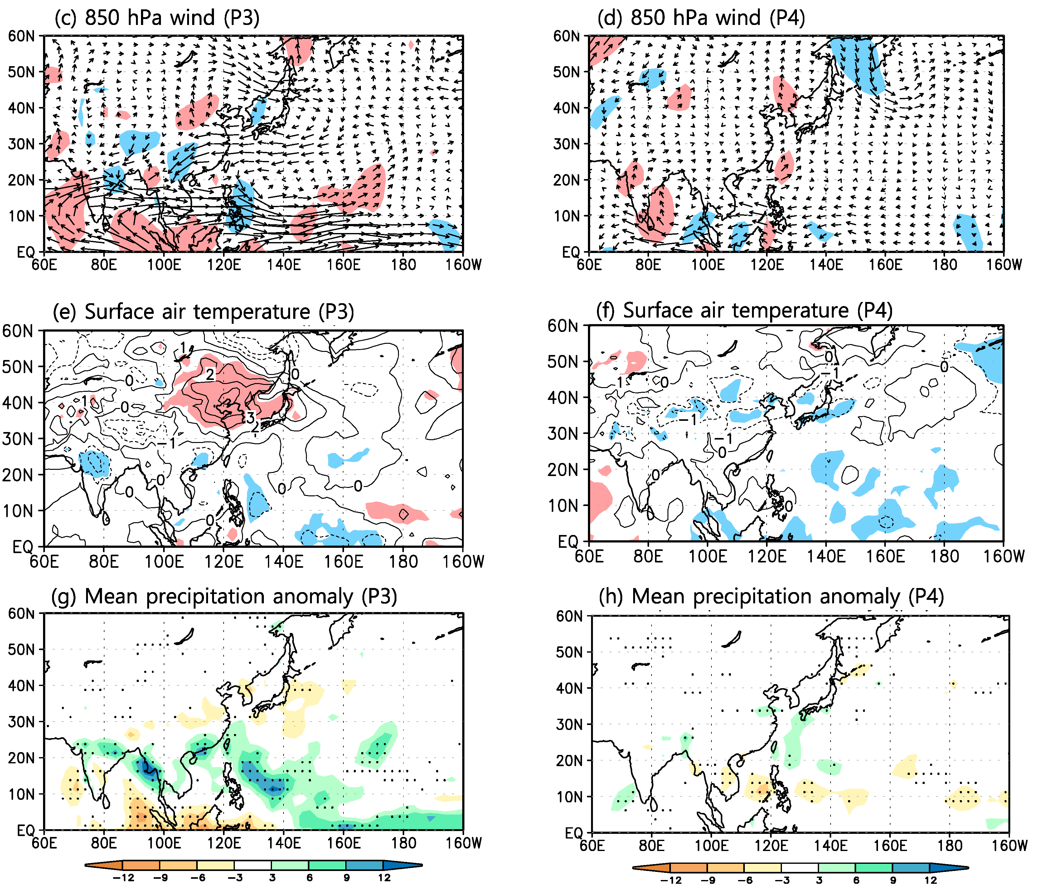
3.2. Changed Influence of the EASMI on the East Asian Summer Circulation

We found that the relationship between tropical IO-EASM is revisited for 1991–1999 (P3) and a decadal change is observed in these relationships for 1991–1999 (P3) and 2000–2016 (P4). In this part, we show the changes in interannual variability of atmospheric circulation regressed to the EASMI. The high pass filtered atmospheric circulation anomalies are the geopotential height at 500 hPa, zonal and meridional wind at 850 hPa, surface air temperature and precipitation. The significance are described by shading in the geopotential height, wind, surface air temperature field and dot in the precipitation field and they are computed in each period with Student’s t-test used when the number of samples is unequal. Non-shaded and non-dotted area fails to pass a field significance test at the 10% level and less than 10% of the area passes the 0.1 p-value of the t-test [31]. However, due to lack of a large enough sample size, we realized that the existence of areas passing significant tests is only considered. In 1991–1999, the regression pattern of 500 hPa geopotential height displays significant negative-positive-negative anomalies as tripolar patterns over East Asia (Figure 4a), such as the East Asia-Pacific (EAP) teleconnection pattern [32,33]. In addition, the negative anomalies in the WNP region are associated with the weakened WNPSH. Compared with patterns in 1979–1990 (not shown), however, negative anomalies are weaker and the centers of significant positive anomalies move westward to Northeast China with stronger and more significant tripolar patterns during the period P3. The regression patterns of wind vector at 850 hPa show an anomalous cyclone over the WNP region and an anticyclone over the region encompassing Korea, Northeast China and Japan (Figure 4c). The patterns of geopotential height and wind in Figure 4a,c seem to satisfy the vertically barotropic structure over the tripolar region. In addition, the westerly wind over the tropical IO and western Pacific is stronger and more significant than in 1979–1990 (not shown). At the surface, significant warm air temperature anomalies are found over the Northeast China and negative anomalies are found over the western Pacific (Figure 4e). This surface air temperature structure generates the stronger land-sea thermal contrast. In the precipitation, the PJ pattern is displayed with the wet WNP and dried East Asia including Korea, Japan and Northeast China. In addition, the drying anomalies are located in the eastern and northern Indian Ocean (Figure 4g).

In contrast, during the period of P4 (2000–2016), the regression patterns show distinctly different features from those of the period P3 (1991–1999). The tripolar pattern of the regressed 500 hPa geopotential height disappears and the negative anomalies appear over WNP and North Pacific (NP) region (Figure 4b). In particular, areas with negative anomalies in the WNP region are reduced in the zonal direction and the intensity of these significant anomalies decreases. At 850 hPa, only anomalous cyclones are observed over the WNP region and the anomalous anticyclone over Korea, Northeast China and Japan disappears. Furthermore, there is westerly wind in the region from eastern IO to the western Pacific (Figure 4d). However, the significant areas are reduced and their intensities seem to be weaker than those in P3 (Figure 4c). The regression pattern of the surface air temperature exhibits few significant patterns (Figure 4f). In the precipitation, the PJ pattern disappears and the dried areas expand to all of the India. In other words, the summer circulation patterns, which are related to EASMI, have completely different structures for 1991–1999 and 2000–2016, especially in the region encompassing Korea, Northeast China and Japan (Figure 4h).

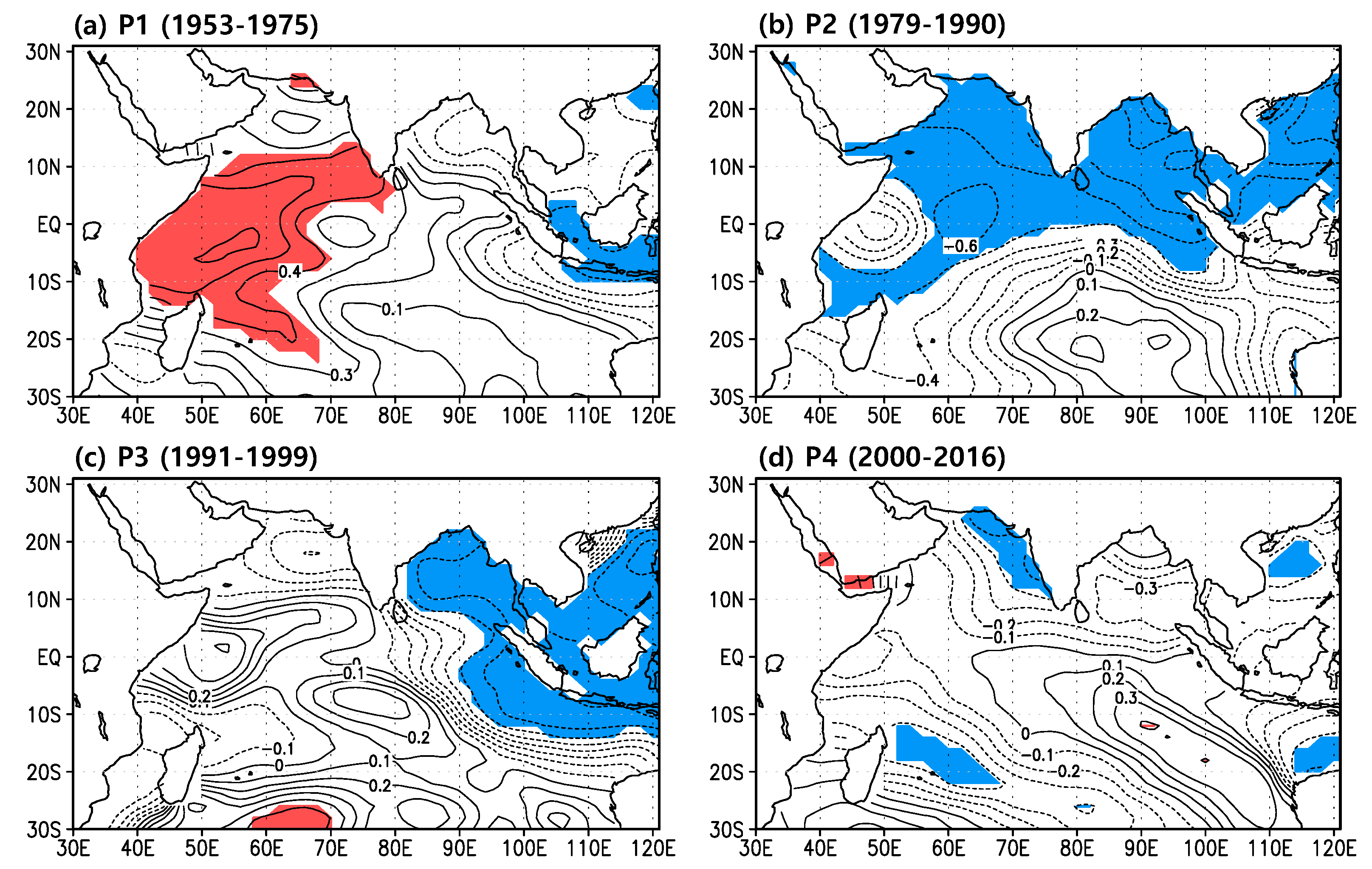
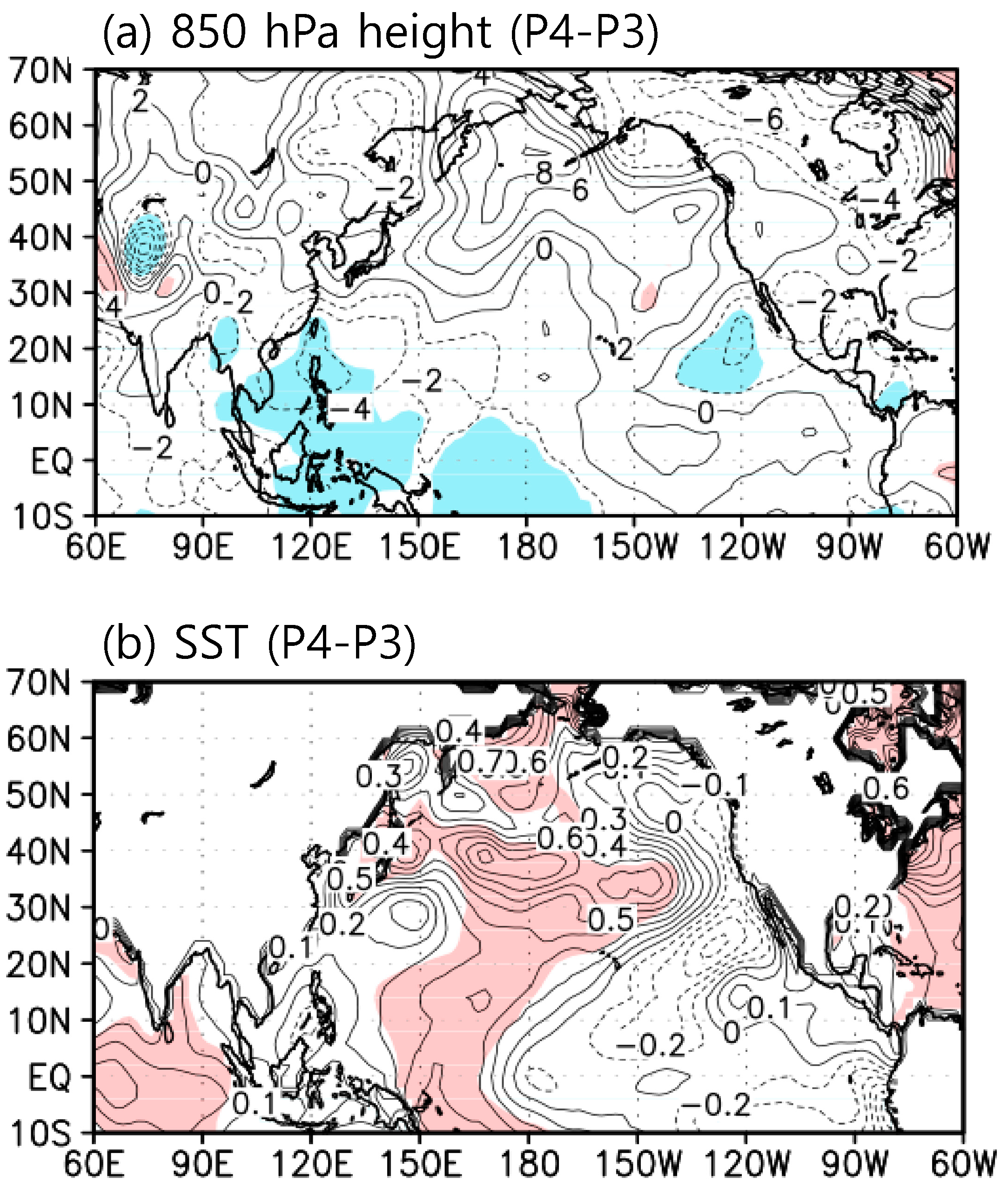
3.3. Influence of the IO SSTA Patterns on Summer Circulation Anomalies in East Asia

As we mentioned in Figure 3, there are changes in the relationships between EASM and two major IO SSTA patterns. In this part, we account for the responses of the East Asian summer circulation anomalies to the discernible SSTA pattern in the tropical IO during the periods 1991–1999 (P3) and 2000–2016 (P4). To clarify the impact of IOD on the East Asia summer circulation, we select the 15 high-IODI and 17 low-IODI event years with ±0.7 standard deviations of IODI for the entire period (1953–2016). The two (1994 and 1997) and five (2003, 2007, 2008, 2012 and 2015) high summer IODI years are included in the periods P3 and P4, respectively. The four (1992, 1995, 1996 and 1998) and five (2001, 2002, 2013, 2014 and 2016) low summer IODI years are included in the periods P3 and P4, respectively. Figure 5 represents 500 hPa geopotential height, 850 h Pa wind, surface air temperature and precipitation field during strong positive IOD events in P3 and P4. For the period P3 (1991–1999), the 500 hPa height pattern reflected by strong positive IOD events exhibits a negative-positive-negative tripolar pattern over East Asia, which is similar to the EAP or PJ pattern (Figure 5a). Although the negative anomalies of the tripolar pattern show small significance unlike positive anomalies, the center positions of the anomalies are located in the same positions as those in Figure 4a. In the 850 hPa wind, the anomalous anticyclone is located over Northeast Asia and a cyclone associated with the WNPSH is located over the WNP region. In addition, strong anomalous westerly wind appears in the IO and western Pacific (Figure 5c). The surface air temperature pattern shows notable warming over Northeast Asia with a strong large land-sea thermal contrast and significant cooling anomalies over the land region of India and the maritime continent (Figure 5e). As a result, this thermal contrast drives the strengthening monsoon system. The precipitation pattern reflected by strong positive IOD events exhibits the PJ pattern (Figure 5g). These composite difference patterns are quite similar to circulation patterns reflected by EASMI shown in the left panels of Figure 4. This confirms that there is a positive relationship between the EASMI and IOD pattern during the period P3.

In the 2000s, the composite difference patterns differ from the patterns for period P3. The only negative anomalies are observed in central western China in the 500 hPa height (Figure 5b). However, there are no significant circulation flow, surface air temperature, precipitation anomalies (Figure 5d,f,h). This indicates that the variability of IOD events is similar to that of the EASMI during P3, not P4. This suggests that the decadal change of ocean-atmosphere system can affect and alter the interannual relationship between the tropical IO and EASM.

Based on the same method used to select IODI event years, we choose high-NIOI and low-NIOI event years for applying the composite difference method. However, in the height, wind, surface air temperature and precipitation patterns, there are no similar patterns in the Figure 4 and no significant pattern over East Asia (not shown). The features of these patterns suggest that NIO events are not significantly associated with the EASM and other factors would be related to EASMI, not SSTA patterns over the IO.

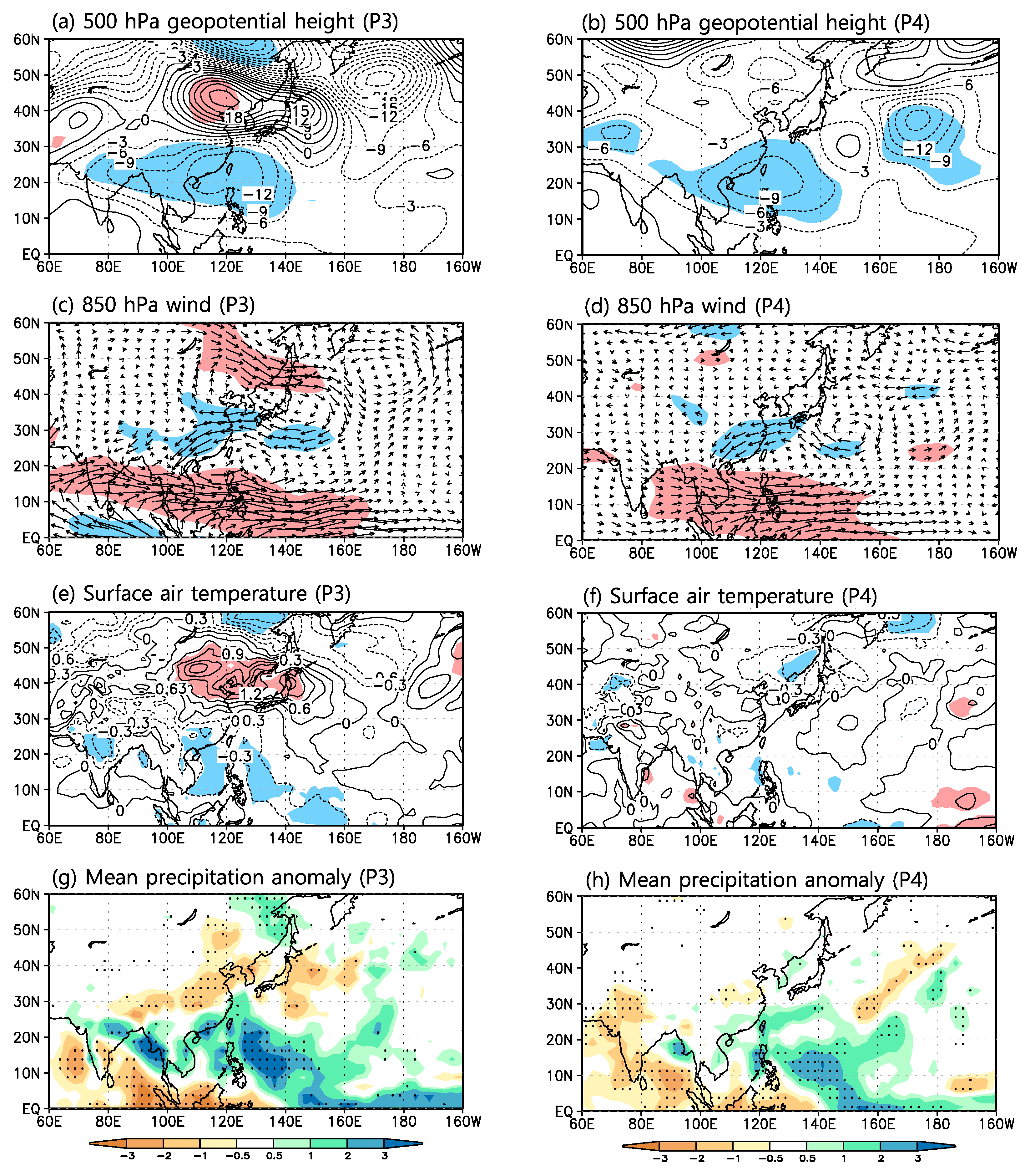
4. Possible Causes for the Change in Relationship between Tropical IO and EASM

The EASM has been affected by various forcing that combine local forcing [34] and lots of remote forcing. In the remote forcing, representatively, SST patterns in the Pacific [13,14,15,16], spring Atlantic [35,36] and May Arctic Oscillation (AO), which modulates the WNPSH [20], are included. Warming in the tropical IO operates like a capacitor, causing the atmospheric anomalies in the Indo-western Pacific and Kelvin wave anchored by atmospheric anomalies suppresses the convection in the subtropical WNP region which has strong relationship with EASM [37]. In Figure 4 and Figure 5, we represent the atmospheric circulation patterns that are associated between EASM and tropical IO. Besides, we find marginally significant decadal and interdecadal changes in the relationship between the tropical SSTA and EASM for 1953–2016 with a decreased relationship after 2000.

The spring NAO which is another remote forcing can lead summer time SST patterns to display tri-pole structures in the North Atlantic and this SST pattern plays a key role in linking the EASM and NAO via subpolar teleconnection, such as Atlantic-Eurasian wave train [35,36]. For identifying spring NAO, the monthly NAO index derived from Climate Prediction Center (CPC)-NOAA data is used. Figure 6 shows the correlation distributions between the 500 hPa stream function and EASMI in the Atlantic and Eurasia during P3 and P4. In the P3 (Figure 6a), a wave train at north of 40° N appears from the North Atlantic to East Asia and the significant positive anomalies are located in the North Atlantic, Ural Mountains and Okhotsk Sea. These positions of positive anomalies are nearly similar to the Atlantic-Eurasian wave train which was mentioned in previous study [36], Figure 2b. However, in the P4, outstanding wave pattern disappears at north of 40° N. Therefore, the spring NAO affects EASM during 1991–1999 and conversely has weak relationship with EASM for 2000–2016.

The question of which factors contribute towards weakening the relationship between the EASMI and tropical IO SSTA remains to be addressed. As mentioned above, the present study intends to distinguish between remote forcing and local forcing. One possible cause is an enhancement in local forcing, such as the land-sea thermal contrast, which is a fundamental mechanism. In order to explore the change in the background state of the ocean-atmosphere system associated with change in intensity of local forcing in EASM, we depict composite differences of summertime surface air temperature of 2000–2016 and 1991–1999 (Figure 7). The significant positive anomalies are located in North China and negative anomalies are located in the Ocean over the WNP region. This structure strengthens EASM and the thermal contrast between land and sea surrounding EASM region has increased since 2000, comparing with that in 1980–1999 [38]. Due to the enhanced direct effect of local forcing on EASM, the relationship between tropical IO SSTA (spring NAO) and EASM has weakened relatively since 2000.

Because the ENSO plays a key role in linking the atmosphere-ocean coupled system with interannual variability mode [16], the low-frequency (LF)-type and the quasi-biennial (QB)-type ENSOs, which have been classified in many previous studies [39,40,41], two types ENSOs are analyzed in terms of association to EASMI for other possible causes. To investigate the change in climate circulation influenced by El Niño events, we show the summertime 850 hPa geopotential height and SSTA corresponding to the composite differences between P3 and P4 (Figure 8). We explore composite differences instead of those only during the ENSO events to prevent losing data. Besides, the interannual variability of circulation over the Pacific is affected dominantly and described by ENSO events. Therefore, Figure 8b is very similar to the composite difference pattern in the Pacific during El Niño events of 2000–2016 (P4) and 1991–1999 (P3) (not shown). The 850 hPa height represents strengthened North Pacific subtropical high and significantly weakened WNPSH (Figure 8a). Besides, there are significant warming over the middle- and higher-latitude Pacific and tropical IO, except for the tropical eastern Pacific including parts of the central Pacific (Figure 8b). Furthermore, even in the previous wintertime, the composite difference of SSTA does not show specific significant patterns in the tropical eastern IO and central IO (not shown). In other words, the changes in Central Pacific-El Niño/Eastern Pacific-El Niño are not outstanding for 1991–1999 (P3) and 2000–2016 (P4). Instead, the summer atmospheric circulation opposite to those shown in Figure 8a has been observed when a warm LF-type ENSO event is dominant [42], Figure 2f. Thus, the LF ENSO is associated with the obvious distinction in the Pacific during P3 and P4. Moreover, the atmospheric circulation patterns when the LF- and QB- type ENSO are dominant are similar to those reflected by EASMI during P3 (Figure 4a,c) and P4 (Figure 4b,d), respectively [42], Figure 2e,f.

In order to compare with the variability and intensity of each type of ENSO, we quantified their monthly indices (Figure 9). These indices are defined by Niño 3.4 index applying band-pass filtering with 16–36 months period in QB- type ENSO index and 42–86 months period in LF-type ENSO index [42]. Some studies have reported an inverse relationship between the ISM and ENSO, which has been weakened rapidly, while the relationship between the EASM and ENSO has enhanced since the late 1970s [43,44,45,46,47]. Therefore, we would focus on the time series of QB and LF-type ENSO after the late 1970s. In the QB-type ENSO, the variability and intensity persist after the late 1970s. On the contrary, the variability of the LF-type ENSO sharply decreases after 2000 and the intensity of the index is weaker than in 1979–1999. Therefore, the QB-type ENSO is more dominant than LF-type ENSO after 2000 and is associated with EASM circulation due to the weakened LF-type ENSO during P4. Furthermore, the LF-type ENSO does not exhibit the features related with “ENSO episodes,” which are represented by the biennial mode, whereas the amplitude of LF-type ENSO is similar to those of biennial ENSO [48]. Therefore, it can be seen from Figure 8 and Figure 9 that the other possible cause is the decreased intensity of low-frequency (LF)-type ENSO. These results suggest the weakened relationship between EASM and tropical IO is contributed by strengthened local forcing and enhanced biennial remote forcing from the Pacific after 2000.

5. Discussion and Conclusions

In this study, we investigated the decadal changes in the relationship between EASMI and the tropical IO SSTA for the summertime from 1953–2016. The entire period can be divided into four parts based on distinct shifts in the relationship. In the periods of 1953–1975 (P1) and 1991–1999 (P3), the positive IOD-like pattern related to the EASMI is dominant over the tropical IO. There is a negative NIO-like pattern associated with the EASMI over the IO for 1979–1990 (P2). In addition, the anomalous SST pattern over the tropical IO influences the EASM via anomalous WNP circulation. On the other hand, for 2000–2016 (P4), the EASMI has a weak relationship with tropical IO SSTA patterns such as IOD and NIO mode. This means that the relationship between tropical IO-EASM is weakened and another factor is likely responsible for the change.

From the present study, it is noted that one possible factor for the change in the relationship between the tropical IO and EASM is the enhanced influence of local forcing on EASM. Remote forcing and local forcing have influenced the EASM. The large land-sea thermal contrast as a local forcing of EASM has been selectively dominated. Compared with distribution of surface air temperature for 1991–1999 (P3), the land-sea thermal contrast during the period of P4 is large and the influence of local forcing is enhanced. Due to enhanced direct influence of local forcing on EASM, the relationship between tropical IO SSTA and EASM has relatively decreased since 2000. The other possible factor for the change in relationship is the decreased intensity of LF-type ENSO. Between the periods P3 and P4, the largest difference in the circulation is associated with circulation patterns opposite to those in the LF-type ENSO events. Furthermore, when the LF-type ENSO is dominant, the circulation patterns are related to those with respect to EASMI during period P3. When the QB-type ENSO is dominant, the circulations are associated with those reflected by the EASMI during period P4. In terms of the LF and QB-type ENSO indices, the intensity of the LF-type ENSO sharply weakens after 2000, unlike the persistent QB-type ENSO. In other words, due to the weakened intensity of the LF-type ENSO, the EASMI is relatively associated with the QB-type ENSO and the relationship between EASM and tropical IO SSTA has decreased relatively since 2000.

Global warming and anthropogenic forcing are likely responsible for the steady weakening of the circulation [49,50]. In particular, the EASMI used in this study is defined by the seasonal difference of low-level wind at 850 hPa. Therefore, we need to reconfirm the indices, which have been defined by the wind field and challenge to involve the changes in circulation over the East Asia such as modulation of WNPSH with the warmer land and warm oceans and westward extension of WNPSH, in the future studies [25,51]. Additionally, because there are active interactions between remote forcing, we need to understand the independence and importance of the tropical IO effect [52,53].

References

1. Lau, K.M.; Yang, S. Climatology and interannual variability of the Southeast Asian summer monsoon. Adv. Atmos. Sci. 1997, 14, 141–162. [Google Scholar] [CrossRef]
2. Ding, Y.H.; Chan, J.C.L. The East Asian summer monsoon: An overview. Meteorol. Atmos. Phys. 2005, 89, 117–142. [Google Scholar] [CrossRef]
3. Murakami, T.; Matsumoto, J. Summer monsoon over the Asian continent and the Western North Pacific. J. Meteorol. Soc. Jpn. 1994, 72, 719–745. [Google Scholar] [CrossRef]
4. Ha, K.J.; Lee, J.Y.; Wang, B.; Xie, S.P.; Kitoh, A. Asian Monsoon Climate Change—Understanding and Prediction. Asia Pac. J. Atmos. Sci. 2017, 53, 179–180. [Google Scholar] [CrossRef]
5. Moon, S.Y.; Ha, K.J. Temperature and Precipitation in the context of the annual cycle over Asia: Model evaluation and future change. Asia Pac. J. Atmos. Sci. 2017, 53, 229–242. [Google Scholar] [CrossRef]
6. Huang, R.; Chen, J.; Wang, L.; Lin, Z. Characteristics, processes, and causes of the spatio-emporal variabilities of the East Asian monsoon system. Adv. Atmos. Sci. 2012, 29, 910–942. [Google Scholar] [CrossRef]
7. Lau, K.M. East Asian summer monsoon rainfall variability and climate teleconnection. J. Meteorol. Soc. Jpn. 1992, 70, 211–242. [Google Scholar] [CrossRef]
8. Wang, B.; Bao, Q.; Hoskins, B.; Wu, G.; Liu, Y. Tibetan Plateau warming and precipitation changes in East Asia. Geophys. Res. Lett. 2008, 35, L14702. [Google Scholar] [CrossRef]
9. Wang, B.; Wu, R.; Fu, X. Pacific-East Asian teleconnection: How does ENSO affect East Asian climate? J. Clim. 2000, 13, 1517–1536. [Google Scholar] [CrossRef]
10. Wu, R.; Hu, Z.Z. Evolution of ENSO-Related Rainfall Anomalies in East Asia. J. Clim. 2003, 16, 3742–3758. [Google Scholar] [CrossRef]
11. Shen, S.; Lau, K.M. Biennial oscillation associated with the East Asian summer monsoon and tropical sea surface temperatures. J. Meteorol. Soc. Jpn. 1995, 73, 105–124. [Google Scholar] [CrossRef]
12. Chang, C.P.; Zhang, Y.S.; Li, T. Interannual and interdecadal variations of the East Asian summer monsoon and tropical Pacific SSTs. Part I: Roles of the subtropical ridge. J. Clim. 2000, 13, 4310–4325. [Google Scholar] [CrossRef]
13. Liu, X.; Yanai, M. Influence of Eurasian spring snow cover on Asian summer rainfall. Int. J. Climatol. 2002, 22, 1075–1089. [Google Scholar] [CrossRef] [Green Version]
14. Wu, G.X.; Liu, Y.M.; Li, W.P. Impacts of the sea surface temperature anomaly in the Indian Ocean on the subtropical anticyclone over the western Pacific? Two-stage thermal adaptation in the atmosphere. Acta Meteorol. Sin. 2000, 58, 513–522. [Google Scholar]
15. Huang, R.H.; Wu, Y.F. The influence of ENSO on the summer climate change in China and its mechanism. Adv. Atmos. Sci. 1989, 6, 21–32. [Google Scholar] [CrossRef]
16. Zhang, R.H.; Sumi, A.; Kimoto, M. Impact of El Niño on the East Asian monsoon. J. Meteorol. Soc. Jpn. 1996, 74, 49–62. [Google Scholar] [CrossRef]
17. Lau, K.M.; Weng, H.Y. Coherent modes of global SST and summer rainfall over China: An assessment of the regional impacts of the 1997/98 El Niño. J. Clim. 2001, 14, 1294–1308. [Google Scholar] [CrossRef]
18. Oh, H.; Ha, K.J. Thermodynamic characteristics and responses to ENSO of dominant intraseasonal modes in the East Asian summer monsoon. Clim. Dyn. 2015, 44, 1751–1766. [Google Scholar] [CrossRef]
19. Gong, D.Y.; Zhu, J.; Wang, S. Significant relationship between spring AO and the summer rainfall along the Yangtze River. Chin. Sci. Bull. 2002, 47, 948–952. [Google Scholar] [CrossRef]
20. Gong, D.Y.; Ho, C.H. Arctic oscillation signals in the East Asian summer monsoon. J. Geophys. Res. 2003, 108, 4066. [Google Scholar] [CrossRef]
21. Ding, R.Q.; Ha, K.J.; Li, J.P. Interdecadal shift in the relationship between the East Asian summer monsoon and the tropical Indian Ocean. Clim. Dyn. 2010, 34, 1059–1071. [Google Scholar] [CrossRef]
22. Hu, Z.Z. Interdecadal variability of summer climate over East Asia and its associated with 500 hPa height and global sea surface temperature. J. Geophys. Res. 1997, 102, 19403–19412. [Google Scholar] [CrossRef]
23. Wu, R.; Wang, B. A contrast of the east Asian summer monsoon-ENSO relationship between 1962–77 and 1978–93. J. Clim. 2002, 15, 3266–3279. [Google Scholar] [CrossRef]
24. Zhu, J.; Huang, D.Q.; Qian, Y.F.; Lin, H.J. Uneven characteristics of warm extremes during Meiyu period over Yangtze-Huaihe region and its configuration with circulation systems (in Chinese). Chin. J. Geophys. Chin. 2010, 53, 2310–2320. [Google Scholar] [CrossRef]
25. Huang, Y.; Wang, B.; Li, X.; Wang, H. Changes in the influence of the western Pacific subtropical high on Asian summer monsoon rainfall in the late 1990s. Clim. Dynam. 2018, 51, 443–455. [Google Scholar] [CrossRef]
26. Li, J.P.; Zeng, Q.C. A unified monsoon index. Geophys. Res. Lett. 2002, 29, 1274. [Google Scholar] [CrossRef]
27. Wang, B.; Wu, Z.; Li, J.; Liu, J.; Chang, C.-P.; Ding, Y.; Wu, G. How to measure the strength of the East Asian summer monsoon. J. Clim. 2008, 21, 4449–4462. [Google Scholar] [CrossRef]
28. Saji, N.H.; Goswami, B.N.; Vinayachandran, P.N.; Yamagata, T. A dipole mode in the tropical Indian Ocean. Nature 1999, 401, 360–363. [Google Scholar] [CrossRef] [PubMed]
29. Du, Y.; Xie, S.P.; Huang, G.; Hu, K. Role of Air-Sea Interaction in the Long Persistence of El Niño-Induced North Indian Ocean Warming. J. Clim. 2009, 22, 2023–2038. [Google Scholar] [CrossRef]
30. Xie, S.P.; Deser, C.; Vecchi, G.A.; Ma, J.; Teng, H.; Wittenberg, A.T. Global Warming Pattern Formation: Sea Surface Temperature and Rainfall. J. Clim. 2009, 23, 966–986. [Google Scholar] [CrossRef]
31. Livezey, R.E.; Chen, W.Y. Statistical Field Significance and its Determination by Monte Carlo Techniques. Mon. Weather Rev. 1983, 111, 46–59. [Google Scholar] [CrossRef] [Green Version]
32. Nitta, T. Convective activities in the tropical western Pacific and their impact on the Northern Hemisphere summer circulation. J. Meteorol. Soc. Jpn. 1987, 64, 373–390. [Google Scholar] [CrossRef]
33. Huang, R.H.; Sun, F.Y. Impact of the tropical western Pacific on the East Asian summer monsoon. J. Meteorol. Soc. Jpn. 1992, 70, 243–256. [Google Scholar] [CrossRef]
34. Webster, P.J.; Magana, V.O.; Palmer, T.N.; Shukla, J.; Tomas, R.A.; Yanai, M.; Yasunari, T. Monsoons: Processes, predictability, and the prospects for prediction. J. Geophys. Res. 1998, 103, 14451–14510. [Google Scholar] [CrossRef] [Green Version]
35. Wu, Z.; Wang, B.; Li, J.; Jin, F.F. An empirical seasonal prediction model of the East Asian summer monsoon using ENSO and NAO. J. Geophys. Res. 2009, 114. [Google Scholar] [CrossRef]
36. Wu, Z.; Li, J.; Jiang, Z.; He, J.; Zhu, X. Possible effects of the North Atlantic Oscillation on the strengthening relationship between the East Asian Summer monsoon and ENSO. Int. J. Climatol. 2012, 32, 794–800. [Google Scholar] [CrossRef]
37. Xie, S.P.; Hu, K.; Hafner, J.; Tokinaga, H.; Du, Y.; Huang, G.; Sampe, T. Indian Ocean Capacitor Effect on Indo-Western Pacific Climate during the Summer following El Niño. J. Clim. 2008, 22, 730–747. [Google Scholar] [CrossRef]
38. Sun, Y.; Ding, Y. Responses of south and east Asian summer monsoons to different land-sea temperature increases under a warming scenario. Chin. Sci. Bull. 2011, 56, 2718–2726. [Google Scholar] [CrossRef]
39. Kim, K.Y.; Kim, Y.Y. Mechanism of Kelvin and Rossby waves during ENSO events. Meteorol. Atmos. Phys. 2002, 81, 169–189. [Google Scholar] [CrossRef]
40. Wang, B.; An, S.I. A method for detecting season-dependent modes of climate variability: S-EOF analysis. Geophys. Res. Lett. 2005, 32, L15710. [Google Scholar] [CrossRef]
41. Bejarano, L.; Jin, F.F. Coexistence of equatorial coupled modes of ENSO. J. Clim. 2008, 21, 3051–3067. [Google Scholar] [CrossRef]
42. Yun, K.S.; Ha, K.J.; Yeh, S.W.; Wang, B.; Xiang, B. Critical role of boreal summer North Pacific subtropical highs in ENSO transition. Clim. Dyn. 2015, 44, 1979–1992. [Google Scholar] [CrossRef]
43. Webster, P.J.; Palmer, T.N. The past and the future of El Niño. Nature 1997, 390, 562–564. [Google Scholar] [CrossRef]
44. Kumar, K.K.; Rajagopalan, B.; Cane, M.A. On the weakening relationship between Indian monsoon and ENSO. Science 1999, 284, 2156–2159. [Google Scholar] [CrossRef] [PubMed]
45. Wang, B.; Huang, F.; Wu, Z.W.; Yang, J.; Fu, X.; Kikuchi, K. Multi-scale Climate Variability of the South China Sea Monsoon: A review. Dynam. Atmos. Oceans 2009, 47, 15–37. [Google Scholar] [CrossRef]
46. Li, J.P.; Wu, Z.W.; Jiang, Z.H.; He, J.H. Can global warming strengthen the East Asian summer monsoon? J. Clim. 2010. [Google Scholar] [CrossRef]
47. Roy, I. Indian Summer Monsoon and El Niño Southern Oscillation in CMIP5 Models: A Few Areas of Agreement and Disagreement. Atmosphere 2017, 8, 154. [Google Scholar] [CrossRef]
48. Rasmusson, E.M.; Wang, X.; Ropelewski, C.F. The biennial component of ENSO variability. J. Mar. Syst. 1990, 1, 71–96. [Google Scholar] [CrossRef]
49. Vecchi, G.A.; Soden, B.J. Global warming and the weakening of the tropical circulation. J. Clim. 2007, 20, 4316–4340. [Google Scholar] [CrossRef]
50. Vecchi, G.A.; Soden, B.J.; Wittenberg, A.T.; Held, I.M.; Leetmaa, A.; Harrison, M.J. Weakening of tropical Pacific atmospheric circulation due to anthropogenic forcing. Nature 2006, 441, 73–76. [Google Scholar] [CrossRef] [PubMed]
51. Yun, K.S.; Yeh, S.W.; Ha, K.J. Covariability of western tropical Pacific-North Pacific atmospheric circulation during summer. Sci. Rep. 2015, 5, 16980. [Google Scholar] [CrossRef] [PubMed] [Green Version]
52. Nicholson, S.E. An analysis of the ENSO signal in the tropical Atlantic and western Indian Oceans. Int. J. Climatol. 1997, 17, 345–375. [Google Scholar] [CrossRef]
53. Alexander, M.A.; Blade, I.; Newman, M.; Lanzante, J.R.; Lau, N.C.; Scott, J.D. The Atmospheric Bridge: The Influence of ENSO Teleconnections on Air-Sea Interaction over the Global Oceans. J. Clim. 2002, 15, 2205–2231. [Google Scholar] [CrossRef]
Figure 1. Time series of normalized (a) EASMI, (b) IODI and (c) NIOI for 1953–2016. Black line represents each index and red line displays their 5-year (from year −2 to year +2 period) running average.
Atmosphere 09 00395 g001
Figure 2. Sliding correlations with (a) 15-year (from year −7 to year +7 period), (b) 11-year (from year −5 to year +5 period) and (c) 7-year (from year −3 to year +3 period) sliding windows between EASMI and indices of the tropical IO SSTA (Black line: NIOI, Green line: IODI line). The dashed red lines represent the significance at the 90% confidence level with the Student’s t-test in each window length.
Atmosphere 09 00395 g002
Figure 3. Correlation distributions of the high pass filtered summer SSTA in the tropical IO with the EASMI in (a) 1953–1975, (b) 1979–1990, (c) 1991–1999, (d) 2000–2016. The contour interval is 0.1 and shading (Red: positive, Blue: negative) shows the significance at the 90% confidence level with the Student’s t-test in each period.
Atmosphere 09 00395 g003
Figure 4. Regression patterns of the high pass filtered summertime 500 hPa height ((a,b), Unit: gpm), 850 hPa wind ((c,d), Unit: m/s), surface air temperature ((e,f), Unit: °C) and precipitation ((g,h), Unit: mm/day) anomalies with respect to the EASMI during the periods P3 and P4. In the height, wind, surface air temperature field, the shaded area denotes the significance at the 90% confidence level with the Student’s t-test in each period length. In the precipitation field, the shaded area indicates value and dotted area denotes the significance at the confidence level with the Student’s t-test in each period length.
Atmosphere 09 00395 g004
Figure 5. Composite differences of the high pass filtered summertime 500 hPa height ((a,b), Unit: gpm), 850 hPa wind ((c,d), Unit: m/s), surface air temperature ((e,f), Unit: °C) and precipitation ((g,h), Unit: mm/day) anomalies between the summer high- and low-IODI during the periods P3 and P4. In the height, wind, surface air temperature field, the shaded areas denote the significance at the 90% confidence level with the Student’s t-test in each period length. In the precipitation field, the shaded areas indicate value and dotted areas denote the significance at the 90% confidence level with the Student’s t-test in each period length.
Atmosphere 09 00395 g005aAtmosphere 09 00395 g005b
Figure 6. Correlation distributions of the high pass filtered summer stream function at 500 hPa with the EASMI in the Atlantic Ocean and Eurasia in (a) 1991–1999 (P3) and (b) 2000–2016 (P4). The contour internal is 0.2 and shading shows the significance at the 90% confidence level of the Student’s t-test.
Atmosphere 09 00395 g006
Figure 7. Composite differences of summertime surface air temperature (Unit: °C) of the periods P4 and P3. The values in the shaded area are significant at the 90% confidence level with the Student’s t-test.
Atmosphere 09 00395 g007
Figure 8. Composite differences of summertime (a) geopotential height at 850 hPa (Unit: gpm), (b) sea surface temperature (Unit: °C) of the periods P4 and P3. The values in the shaded areas are significant at the 90% confidence level with the Student’s t-test.
Atmosphere 09 00395 g008
Figure 9. Interannual variability of (a) QB- and (b) LF-type ENSO. The blue line indicates the wintertime QB- and LF-type ENSO indices and the red line is the 11-year running standard deviation of indices.
Atmosphere 09 00395 g009