Parameterization of the Aerosol Upscatter Fraction as Function of the Backscatter Fraction and Their Relationships to the Asymmetry Parameter for Radiative Transfer Calculations

Abstract

Simple analytical approximations for aerosol radiative forcing generally contain the aerosol upscatter fraction (the fraction of scattered light that is scattered into the upper hemisphere), while ambient measurements generally yield the backscatter fraction, and theoretical calculations of scattering phase functions often yield the asymmetry parameter. Therefore, simple analytical relationships and parameterizations relating these three parameters are very valuable for radiative transfer calculations. Here, we review published parameterizations, mostly based on the Henyey-Greenstein phase function, and evaluate their goodness and range of validity. In addition, we give new parameterizations that are valid over the full range of backscatter fractions that are possibly encountered in the ambient atmosphere (i.e., 0 to 0.5).

1. Introduction

Simple analytical expressions for estimating aerosol radiative forcing are very useful for enhancing our understanding and for determining the influence of particle microphysics and optics on radiative forcing. For an optically thin (aerosol optical thickness τ << 1) aerosol layer, Charlson, et al. [1] have given such an analytical expression for purely scattering aerosols such as sulfate aerosols. Chýlek and Wong [2] extended this expression to absorbing aerosols, yielding a global average of the aerosol radiative forcing ΔF_aer per aerosol optical thickness τ. A slightly modified version of their equation (8) gives ΔF_aer/τ as

$$\frac{\Delta F_{aer}}{\mathsf{\tau }}=-\frac{S_0}{2}{T}_{atm}^2(1-A_{cld})\left[\overline{\mathsf{\beta }}\mathsf{\omega }{\left(1-R_{surf}\right)}^2-2\left(1-\mathsf{\omega }\right)R_{surf}\right]$$

(1)

where S₀ is the solar constant (S₀ = 1370 W/m²), T_atm is the transmittance of the atmosphere above the aerosol layer, A_cld is the fractional cloud cover, ω is the single scattering albedo, R_surf is the surface reflectance, and $\overline{\mathsf{\beta }}$ is the average aerosol upscatter fraction for the earth’s sunlit hemisphere. This equation has also been given without derivation by Haywood and Shine [3]. More recently, this equation has been compared with the output of a global Monte-Carlo Aerosol Cloud Radiation (MACR) model and has been found adequate for cloud-free conditions [4].

Because no direct method for measuring the average aerosol upscatter fraction $\overline{\mathsf{\beta }}$ is available, it needs to be related to a quantity available from measurements such as the aerosol backscatter fraction b or to a quantity available from theory such as the aerosol asymmetry parameter g defined as the intensity-weighted average cosine of the scattering angle θ [5]

$$g=\frac{1}{2}{{\displaystyle \int }}_0^{\mathsf{\pi }}\cos \mathsf{\theta }P\left(\mathsf{\theta }\right)\sin \mathsf{\theta }d\mathsf{\theta }$$

(2)

where P(θ) is the scattering phase function.

2. Average Aerosol Upscatter Fraction

Estimating the global average of the aerosol radiative forcing ΔF_aer per aerosol optical thickness τ with Equation (1) requires knowledge of $\overline{\mathsf{\beta }}$, the average aerosol upscatter fraction for the earth’s sunlit hemisphere. This average upscatter fraction $\overline{\mathsf{\beta }}$ can be written as

$$\overline{\mathsf{\beta }}={{\displaystyle \int }}_0^{\raisebox{1ex}{$\mathsf{\pi }$}\!\left/ \!\raisebox{-1ex}{$2$}\right.}\mathsf{\beta }\left({\mathsf{\theta }}_0\right)\sin {\mathsf{\theta }}_{0}d{\mathsf{\theta }}_0$$

(3)

where β(θ₀) is the upscatter fraction, the fraction of incident solar light that is scattered into the upward hemisphere (i.e., back into space), which is a function of the solar zenith angle θ₀ [6]. The upscatter fraction β(θ₀) is given by an integral over the scattering angles dΩ = sinθ dθ dϕ of the upward hemisphere as [6,7]

$$\mathsf{\beta }\left({\mathsf{\theta }}_0\right)={\left(4\mathsf{\pi }\right)}^{-1}\underset{\begin{array}{c}upward\\ hemisphere\end{array}}{{\displaystyle \int }}P\left(\mathsf{\theta },\mathsf{\varphi }\right)d\mathrm{\Omega }$$

(4)

where P(θ,ϕ) is the phase function depicting the angular distribution of the scattered light normalized to 4π when integrated over all directions, that is

$${{\displaystyle \int }}_{4\mathsf{\pi }}P\left(\mathsf{\theta },\varphi \right)d\mathsf{\Omega }=4\mathsf{\pi }$$

(5)

As shown by Wiscombe and Grams [7] and nicely illustrated by Schwartz [6], the double integral over the two angles dθ dϕ in Equation (4) can be simplified to the sum of two single integrals as

$$\mathsf{\beta }\left({\mathsf{\theta }}_0\right)=\frac{1}{2\mathsf{\pi }}{{\displaystyle \int }}_{\raisebox{1ex}{$\mathsf{\pi }$}\!\left/ \!\raisebox{-1ex}{$2$}\right.-{\mathsf{\theta }}_0}^{\raisebox{1ex}{$\mathsf{\pi }$}\!\left/ \!\raisebox{-1ex}{$2$}\right.+{\mathsf{\theta }}_0}P\left(\mathsf{\theta }\right)\sin \mathsf{\theta }{\cos }^{-1}\left(\cot {\mathsf{\theta }}_0\cot \mathsf{\theta }\right)d\mathsf{\theta }+\frac{1}{2}{{\displaystyle \int }}_{\raisebox{1ex}{$\mathsf{\pi }$}\!\left/ \!\raisebox{-1ex}{$2$}\right.+{\mathsf{\theta }}_0}^{\mathsf{\pi }}P\left(\mathsf{\theta }\right)\sin \mathsf{\theta }d\mathsf{\theta }$$

(6)

Using Equations (3)–(6), the average upscatter fraction $\overline{\mathsf{\beta }}$ for the earth’s sunlit hemisphere, as needed for globally averaged radiative forcing calculations with Equation (1), can be calculated readily if the phase function P(θ) is known.

3. Henyey-Greenstein (HG) Phase Function, Asymmetry Parameter, and Its Range in the Atmosphere

3.1. Henyey-Greenstein (HG) Phase Function and Asymmetry Parameter g

The analytical estimation of the aerosol radiative forcing in Equation (1) depends on the availability of an analytical expression for the phase function. The Henyey-Greenstein (HG) phase function is a commonly used, simple, single parameter, analytical phase function that gives an approximation of the aerosol phase function; it will be used in the following analytical estimations. In principle, the HG phase functions can be used for any kind of aerosols including spherical (homogeneous and non-homogeneous, including layered) and non-spherical aerosols. It does not directly account for any microphysical particle properties including size, morphology, and complex refractive index. Instead, the HG phase function P_HG(θ) uses a single parameter, the scattering asymmetry parameter g to describe the angular distribution of the scattered light as [8,9,10]

$$P_{HG}(\mathsf{\theta })=\frac{1-g^2}{{(1+g^2-2g\cos \mathsf{\theta })}^{\raisebox{1ex}{$3$}\!\left/ \!\raisebox{-1ex}{$2$}\right.}}$$

(7)

The asymmetry parameter g needed to obtain the HG phase function can be obtained from ambient atmospheric measurements or from calculations such as Mie theory for homogeneous spherical particles or more involved calculations including T-matrix or coupled dipole-dipole theory for non-spherical and non-homogeneous particles [11]. Comparisons of the HG phase function with Mie theory phase functions and its shortcomings for aerosol radiative forcing calculations have been discussed in detail by Marshall, et al. [10] and Boucher [9]. We are not aware of any comparisons of the HG phase function with phase functions calculated for non-spherical and/or non-homogeneous particles

3.2. Range of the Asymmetry Parameter

3.2.1. Principal Considerations

While the scattering asymmetry parameter g can in principle be in the range from −1 (pure backscatter) to +1 (pure forward scatter), negative values of g occur only for small metallic particles [12,13] and are not relevant for the ambient atmosphere. Therefore, only values of the asymmetry parameter g between 0 (symmetric scatter) and +1 (pure forward scatter) need to be considered.

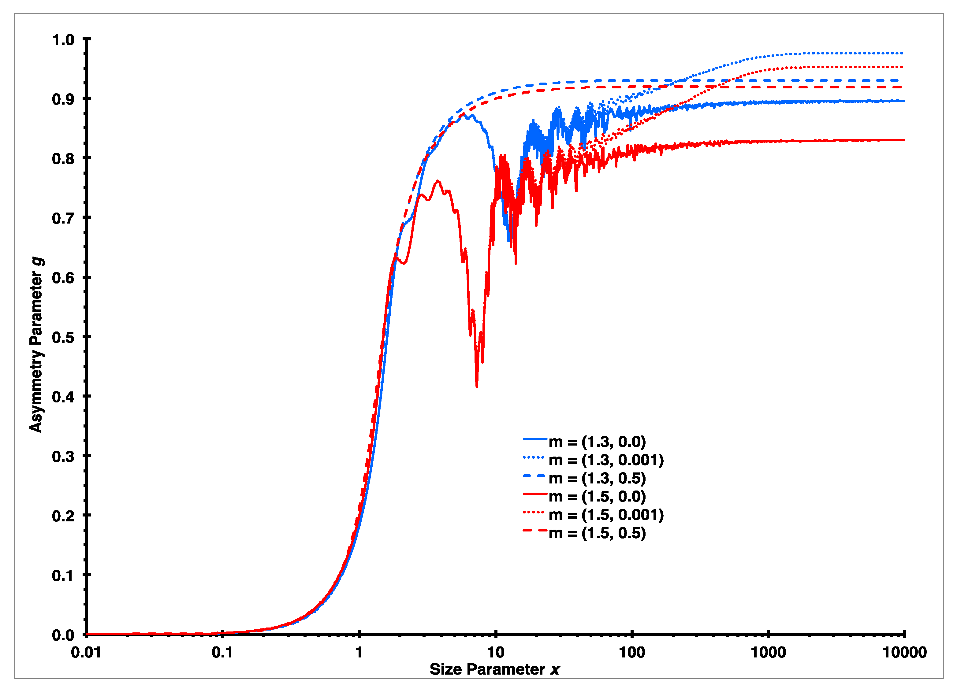
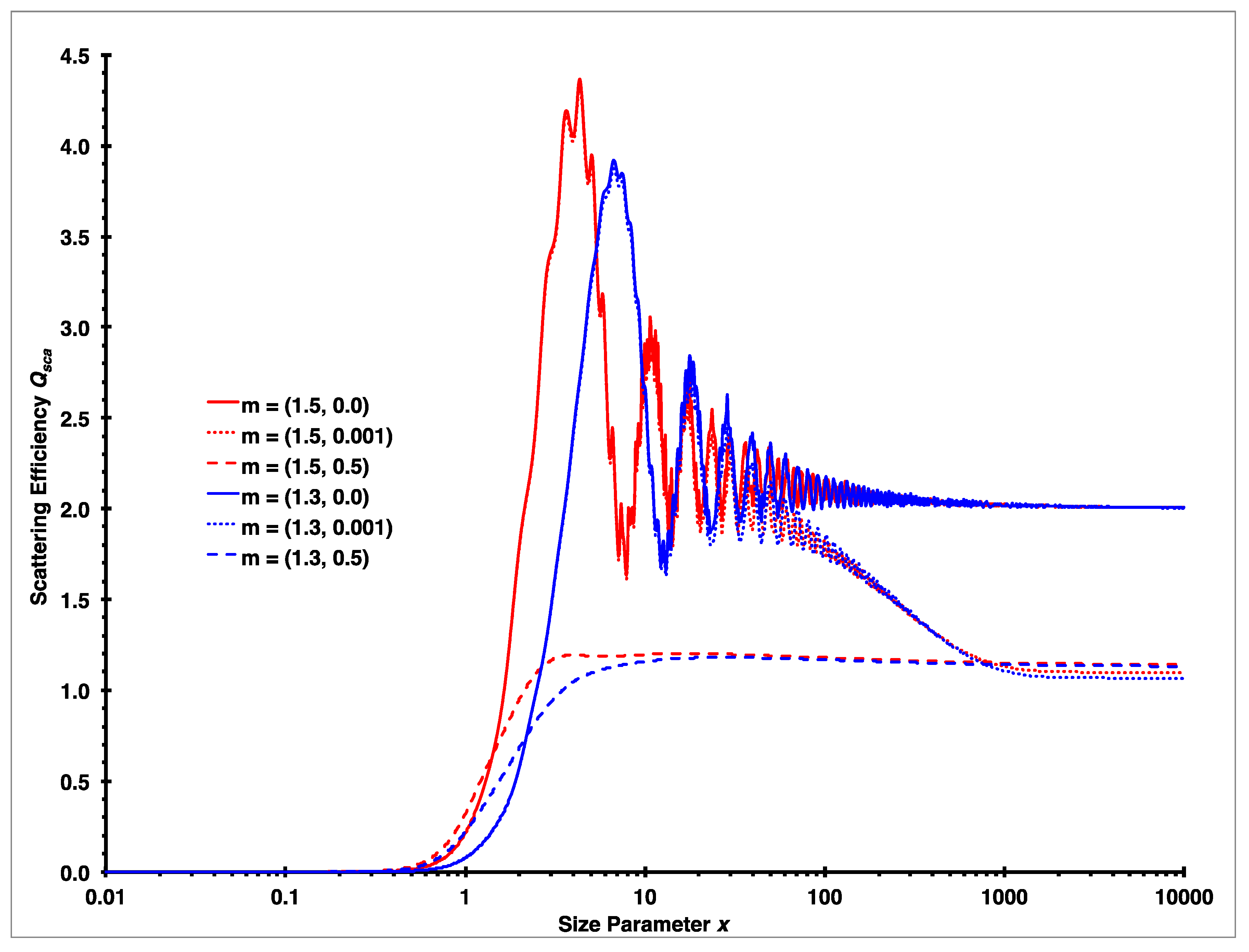
3.2.2. Mie Calculations of the Asymmetry Parameter g

For homogeneous spherical particles, the asymmetry parameter g can be calculated readily using Mie theory [14]. It is a function of particle size parameter x, which is the ratio of particle circumference (i.e., 2πr; r being the particle radius) and wavelength λ (i.e., x = 2πr/λ), and of the complex refractive index m = (n, k), where n is the real part and k the imaginary part of the refractive index. In the visible, the real part of the refractive index of dry ambient aerosols is commonly ~1.5 [15], while for wet aerosols this value is lowered due to mixing with water, which has a refractive index of ~1.3 [16]. Figure 1 shows the asymmetry parameter g as function of size parameter x for all combinations of the real part of the refractive index equal 1.3 and 1.5 and the imaginary part equal 0.0, 0.001, and 0.5.

For all refractive indices considered here, the asymmetry parameter approaches zero for size parameters much below one; this is the typical symmetric scattering in the Rayleigh regime (e.g., [17]). However, these small values of the asymmetry parameter do not contribute much to the scattering of a disperse particle size distribution as found in the atmosphere, because in the Rayleigh regime, scattering efficiencies (the ratio of scattering and geometric cross-section) are proportional to r⁴; very small particles (x << 1) do not contribute much to scattering compared to larger particles. This is illustrated in Figure 2, where the scattering efficiency Q_sca is plotted as a function of size parameter x for different complex refractive indices; clearly particles with x < 1 have a much smaller scattering efficiency than those with x > 3.

For increasing size parameters, both scattering efficiency (Figure 2) and asymmetry parameter (Figure 1) start to quickly increase around x ≈ 1, with the asymmetry parameter showing characteristic oscillations for small imaginary parts of the refractive indices, and approaching an upper limit for large size parameters in the geometric optics regime (x >> 1). As shown in Figure 1, this limit is the largest for small imaginary parts of the refractive index (i.e., k = 0.001), especially when combined with small real parts of the refractive index (e.g., n = 1.3); it is smaller for large imaginary parts of the refractive index (i.e., k = 0.5), and even smaller for zero imaginary parts of the refractive index (i.e., k = 0.0).

In summary, the Mie theory calculations presented here indicate that the upper limit of the asymmetry parameter g for absorbing particles (i.e., 10⁻⁴ < k < 0.1) is g ~ 0.952 for n = 1.5 and g ~ 0.975 for n = 1.3. For non-absorbing particles (i.e., k = 0), these upper limits are substantially smaller with g ~ 0.83 for n = 1.5 and g ~ 0.90 for n = 1.3. While in principle lower limits of the asymmetry parameter g can approach zero for sufficiently small particles, even a minority population of larger particles will result in a substantially larger g because the scattering efficiency for small (x << 1) particles is proportional to x⁴.

3.2.3. Measurements of the Asymmetry Parameter g in the Ambient Atmosphere

Measurements, retrievals, and representative calculations of the scattering asymmetry parameter g in the ambient troposphere are fairly sparse.

The most comprehensive effort establishing an aerosol asymmetry parameter climatology has been made by Fiebig and Ogren [18], who have introduced a novel algorithm that retrieves the asymmetry parameter from an inversion of routinely measured aerosol absorption, scattering, and backscattering coefficients. They have applied this algorithm to data from six stations within the aerosol monitoring network of the NOAA Earth System Research Laboratory to establish an aerosol asymmetry parameter climatology representing dried particles of continental, marine, arctic, and free tropospheric origin in two size ranges, <1 and <10 μm aerodynamic diameter. They observed that the 5-to-95 percentiles of the retrieved asymmetry parameters were always within the 0.36 to 0.71 range [18].

Andrews, et al. [5] derived the Mie-equivalent asymmetry parameter using multiple methods from a large suite of measurements (in situ and remote, from surface and aircraft) made in Oklahoma during the May 2003 aerosol intensive operations period (IOP). Andrews, et al. [5] observed a range of g between 0.5 and 0.8 during this ~1 month IOP.

The third-order polynomial approximation g_{A_fit} (Equation (9)) giving the asymmetry parameter as function of the backscatter fraction b suggested by Arnott [19] and published by Andrews, et al. [5] has been used by Ramachandran and Rajesh [20] and by Gopal, et al. [21] to derive the asymmetry parameter g from nephelometer measurements of b. Ramachandran and Rajesh [20] conducted an airborne campaign measuring vertical profiles in the lower troposphere at four locations in tropical India. They reported a range of g between 0.3 and 0.6 at a wavelength of 550 nm and scaled to a relative humidity (RH) of 30%. Gopal, et al. [21] conducted one year of ground-based nephelometer measurements at Anantapur, a semi-arid region in southern India and reported a range of g between 0.53 and 0.65 at a wavelength of 550 nm.

Formenti, et al. [22] used a Mie algorithm to calculate the asymmetry parameter g from refractive index and aerosol size distribution. For dust episodes encountered on El Pico del Teide, Tenerife, Canari Islands, Spain, they reported g between 0.72 and 0.73.

In addition, we have estimated the range of the atmospheric aerosol asymmetry parameter from published ranges of the aerosol backscatter fraction b using Equation (10) that assumes a Henyey-Greenstein phase function. Measurements include airborne measurements by Hegg, et al. [23] in marine air near the coasts of California and Washington, USA at relative humidity (RH) between 10% and 65% yielding 0.08 ≤ b ≤ 0.20 (i.e., 0.72 ≥ g ≥ 0.44); measurements by Hegg, et al. [24] in the arctic near Prudhoe Bay, Alaska, USA at RH of 30% yielding 0.07 ≤ b ≤ 0.24 (i.e., 0.75 ≥ g ≥ 0.37), ground-based measurements by Ichoku, et al. [25] in the Negev Desert, Israel yielding values generally in the range 0.1 ≤ b ≤ 0.22 (i.e., 0.66 ≥ g ≥ 0.40), multi-year measurements reported by Andrews, et al. ([26]; Figure 3f) for twelve high altitude, northern hemisphere, mid-latitude platforms yielded 5-to-95 percentiles 0.062 ≤ b ≤ 0.31 (i.e., 0.77 ≥ g ≥ 0.26), and four years of hourly measurements of dry-state aerosols at the Global Atmospheric Watch (GAW) observation site Melpitz in East Germany by Ma, et al. [27] yielding 0.075 ≤ b ≤ 0.26 (i.e., 0.73 ≥ g ≥ 0.34). All of these results are in general agreement with the conclusions of Fiebig and Ogren [18] and are summarized in

Table 1. Measurements of the Asymmetry Parameter g in the Ambient Atmosphere.

Range of g	Method	Location	Reference
0.36–0.71	Novel Algorithm	Global NOAA Network	Fiebig and Ogren [18]
0.5–0.8	Mie Retrieval	Oklahoma, USA	Andrews, et al. [5]
0.3–0.6	Nephelometer Retrieval	Tropical India	Ramachandran and Rajesh [20]
0.53–0.65	Nephelometer Retrieval	Southern India	Gopal, et al. [21]
0.72–0.73	Mie Retrieval	Canari Islands, Spain	Formenti, et al. [22]
0.44–0.72	Nephelometer Retrieval	Marine West Coast, USA	Hegg, et al. [23]
0.37–0.75	Nephelometer Retrieval	Prudhoe Bay, AK, USA	Hegg, et al. [24]
0.40–0.66	Nephelometer Retrieval	Negev Desert, Israel	Ichoku, et al. [25]
0.26–0.77	Nephelometer Retrieval	Northern, Mid-Latitudes	Andrews, et al. ([26]; Figure 3f)
0.34–0.73	Nephelometer Retrieval	Melpitz, East Germany	Ma, et al. [27]

.

However, one may speculate about smaller values of g (i.e., closer to 0) for locations near sources of accumulation mode particles and larger values (i.e., closer to one) for locations near sources of large particles (e.g., mineral dust particles). Therefore, all our plots and approximations are given for a more generous range of asymmetry parameters g between 0 and 1.

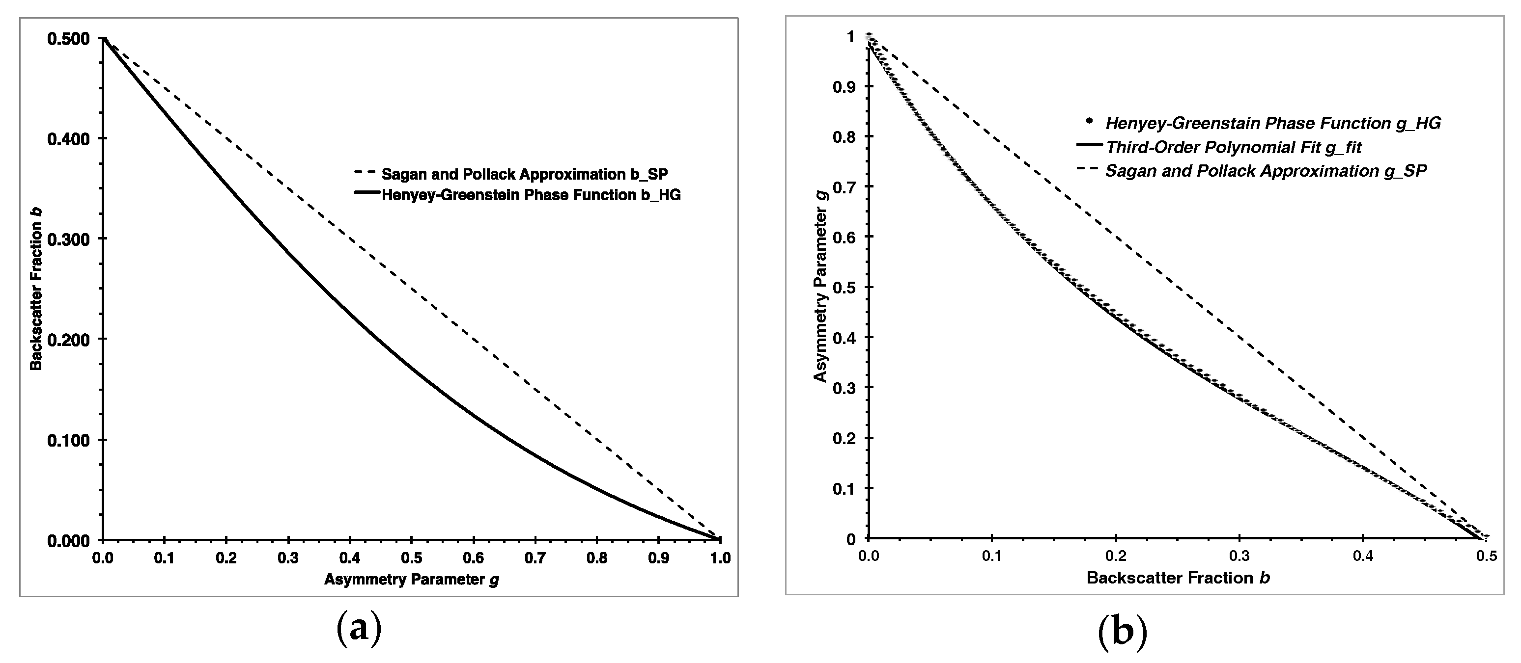
3.3. Backscatter Fraction for Henyey-Greenstein (HG) Phase Function: Solutions and Approximations

The HG phase function can be integrated analytically to yield the backscatter fraction b_HG, which equals the upscatter fraction β_HG(θ₀) for θ₀ = 0 (solar zenith), as [7]

$$b_{HG}={\mathsf{\beta }}_{HG}({\mathsf{\theta }}_0=0)=\frac{1}{2}{{\displaystyle \int }}_{\mathsf{\pi }/2}^{\mathsf{\pi }}{P}_{HG}(\mathsf{\theta })\sin \mathsf{\theta }d\mathsf{\theta }=\frac{1-g^2}{2g}\left(\frac{1}{\sqrt{1+g^2}}-\frac{1}{1+g}\right)$$

(8)

This relationship is plotted in Figure 3a for 0 ≤ g ≤ 1.

Equation (8) gives a fairly simple analytical solution for b_HG(g) with little need for approximations. However, this is not true if the inverse function, g(b_HG) is needed. For this case, Arnott [19], as discussed by Andrews, et al. [5], has suggested a third-order polynomial approximation g_{A_fit} as

$$g_{A\_fit}=-7.143889b_{HG}^3+7.464439b_{HG}^2-3.96356b_{HG}+0.9893$$

(9)

While it is not clear for what range of g and b_HG this approximation was intended, for 0 ≤ b_HG ≤ 0.5, corresponding to 0 ≤ g ≤ 1, this approximation has a root-mean-square error (RMSE) of 0.0055. A slightly better third-order polynomial approximation g_fit can be given with far fewer significant figures as

$$g_{fit}=-6.347b_{HG}^3+6.906b_{HG}^2-3.859b_{HG}+0.9852$$

(10)

with an RMSE of 0.0051. This approximation is shown in Figure 3b together with the exact values of g. The differences between the results of Equations (9) and (10) are very small and would be impossible to distinguish if g_{A_fit} (Equation (9)) would be added to Figure 3b. However, g_fit is a slightly better fit and as additional benefit, uses far fewer significant figures for its coefficients.

Previously, Chýlek and Wong [2] have suggested using a linear approximate relation from Sagan and Pollack [28] to calculate the upscatter fraction (β in their notation; $\overline{\mathsf{\beta }}$ in our notation) as ${\mathsf{\beta }}_{CW}=\left(1-g/2\right)/2$ (Equation (13); [28]). There seem to be two problems with this suggestion: (1) Sagan and Pollack [28] define their β as “a measure of the fraction of radiation singly scattered into the backward hemisphere of the incident radiation.”; this would be the backscatter fraction ($b_{HG}= {\mathsf{\beta }}_{HG}\left({\mathsf{\theta }}_0=0\right)$ in our notation) but not the average aerosol upscatter fraction as apparently assumed by Chýlek and Wong [2]; (2) the equation ${\mathsf{\beta }}_{CW}=\left(1-g/2\right)/2$ as given by Chýlek and Wong [2] contains a typographical mistake [29]; it should be ${\mathsf{\beta }}_{CW}=\left(1-g\right)/2$ as originally given by Sagan and Pollack [28]. In our notation, this can be written as

$$b_{SP}=\left(1-g\right)/2$$

(11)

or inverted as

$$g_{SP}=1-2b$$

(12)

These linear approximations are shown in Figure 3 and the original equation ${\mathsf{\beta }}_{CW}=\left(1-g/2\right)/2$ is included in Figure 4 to make the typographical mistake obvious.

The linear approximation b_SP (Equation (11)) agrees with the exact Equation (8) for g = 0 and g = 1 (see Figure 3a); in between, the linear approximation b_SP is consistently larger (by up to ~0.08) than b_HG (Equation (8)) and has an RMSE of 0.056 for the range of 0 ≤ g ≤ 1. Note that the linear approximation is good for the extreme values of g near 0 and 1 that are not encountered in the ambient atmosphere, but especially poor for the intermediate realistic values [18]. Similarly, the linear approximation g_SP (Equation (12)) given by Sagan and Pollack [28] has an RMSE of 0.11 for the range of 0 ≤ g ≤ 1 but again performs more poorly for realistic ambient values of b and g (see Figure 3b).

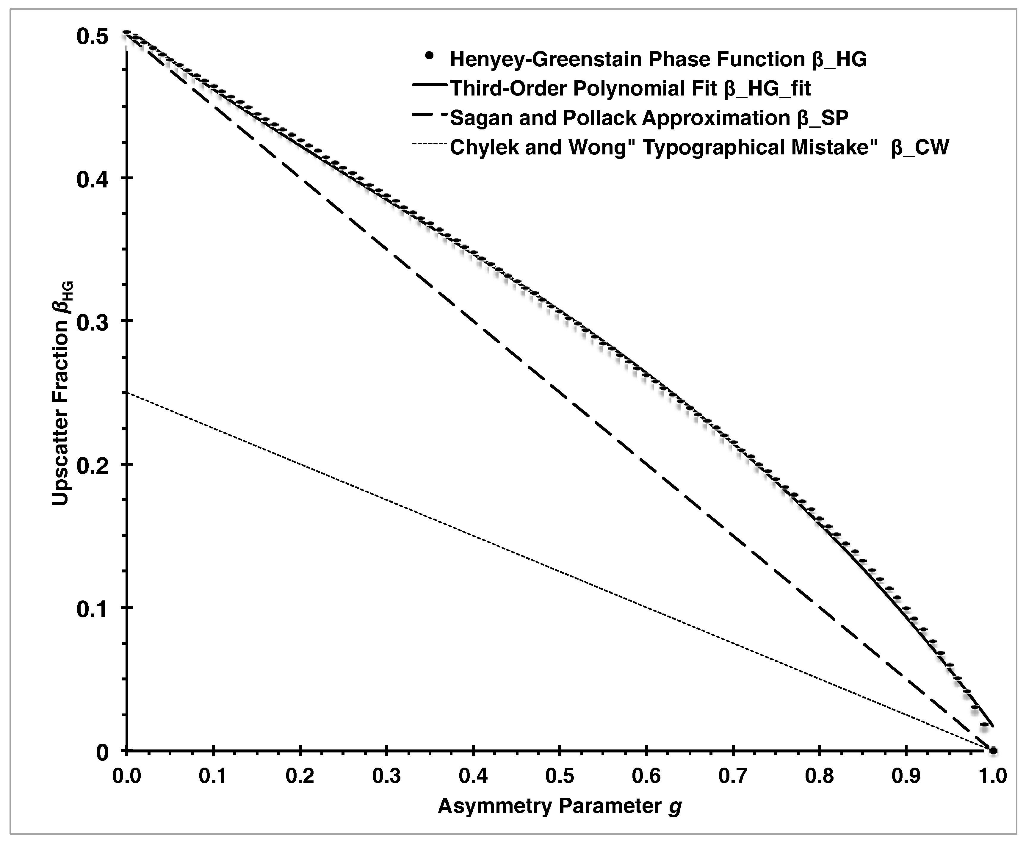
3.4. Upscatter Fraction for Henyey-Greenstein (HG) Phase Function: Solutions and Approximations

The average upscatter fraction $\overline{{\mathsf{\beta }}_{HG}}$ for the sunlit hemisphere using the HG phase function can be directly related to the asymmetry parameter g, which is often employed in radiative transfer models and can be obtained directly from optical scattering calculations such as Mie theory [14] and derived from measurements of aerosol optics and other properties [5]. For the HG phase function, the average upscatter fraction $\overline{{\mathsf{\beta }}_{HG}}$ can be written as a single integral [7]

$$\overline{{\mathsf{\beta }}_{HG}}=\frac{1-g}{2g}\left(-1+\frac{2\left(1+g\right)}{\mathsf{\pi }}{{\displaystyle \int }}_0^{\raisebox{1ex}{$\mathsf{\pi }$}\!\left/ \!\raisebox{-1ex}{$2$}\right.}{(1-g^2{\sin }^2\mathsf{\theta })}^{-0.5}d\mathsf{\theta }\right)$$

(13)

Using this Equation (13), the average upscatter fraction $\overline{{\mathsf{\beta }}_{HG}}$ can be calculated as function of the asymmetry parameter g with results shown in Figure 4.

Equation (13) can be approximated by a third-order polynomial $\overline{{\mathsf{\beta }}_{HG\_fit}}$ for 0 ≤ g ≤ 1 as

$$\overline{{\mathsf{\beta }}_{HG\_fit}}=-0.2936g^3+0.2556g^2-0.4489g+0.5043$$

(14)

with an RMSE of 0.0029. This approximation is shown in Figure 4 as a solid line together with the exact values shown as solid dots and a linear approximation (dashed line) given by Sagan and Pollack [28] originally for the backscatter, but also somewhat useful for the upscatter fraction which has an RMSE of 0.046. In addition, to emphasize the typographical error in the original β_CW found in Chýlek and Wong [2], we have included this curve to make the factor of two difference from the linear approximation (dashed line) given by Sagan and Pollack [28] obvious.

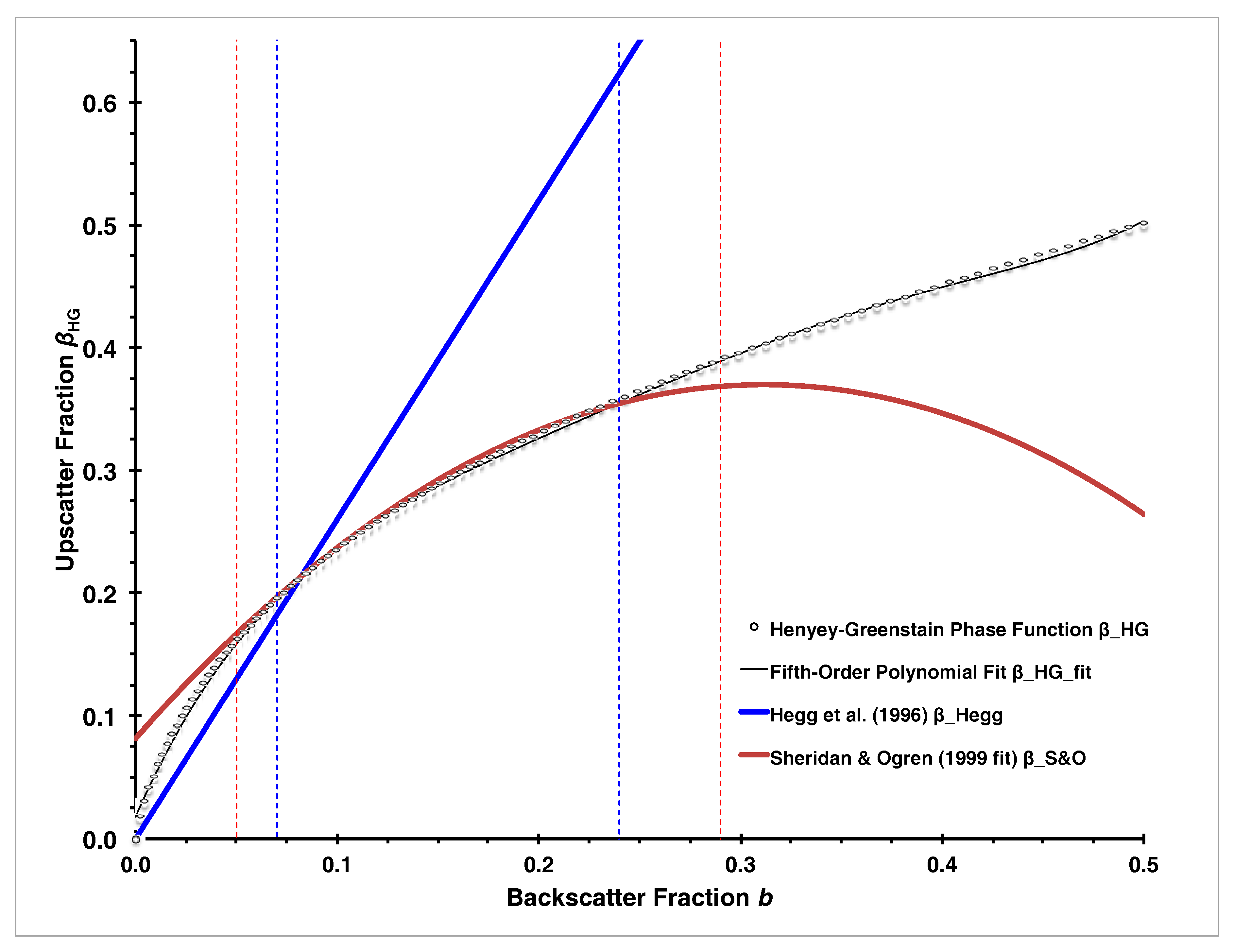
3.5. Relationship and Approximations between Average Upscatter Fraction and Backscatter Fraction for Henyey-Greenstein (HG) Phase Function

While the backscatter fraction can be directly measured with commercial integrating nephelometers [30,31], no such instrument exists for the measurement of the upscatter fraction; therefore a simple relation connecting these two fractions would be very useful for estimating aerosol radiative forcing using Equation (1). Although there is no analytical expression giving the average upscatter fraction $\overline{{\mathsf{\beta }}_{HG}}$ as a function of the backscatter fraction b_HG, we can use a parametric plot with the two fractions expressed as functions of the asymmetry parameter g (Equations (8) and (13)) to show their relationship and to evaluate polynomial fits approximating it. Figure 5 shows this parametric plot with exact values shown as circles for backscatter fractions 0 ≤ b_HG ≤ 0.5, corresponding to 0 ≤ g ≤ 1. A fifth-order polynomial fit $\overline{{\mathsf{\beta }}_{HG\_fit}}$ can be given as

$$\overline{{\mathsf{\beta }}_{HG\_fit}}=99.69b^5-144.6b^4+80.44b^3-22.05b^2+3.73b+0.018$$

(15)

with an RMSE of 0.0031 for 0 ≤ b_HG ≤ 0.5, and is shown as the thin solid black line in Figure 5.

3.5.1. Approximation by Hegg, et al. [24]

Hegg, et al. [24] give the simple linear relationship

$$\overline{{\mathsf{\beta }}_{Hegg}}=2.6b$$

(16)

for their airborne data obtained in the vicinity of Prudhoe Bay, Alaska in June 1995. This Equation (16) has been used by Formenti, et al. [33] to help estimate the sign of aerosol radiative forcing over the Negev Desert (Israel). We plot Equation (16) as a solid blue line in Figure 5 together with the range of the backscatter fraction b encountered by Hegg, et al. [24] indicated by dashed blue vertical lines (i.e., 0.07 ≤ b ≤ 0.24). Their equation is close to the exact HG values near the lower end of this range but nearly a factor of two higher at the upper end, with an RMSE of 0.33.

3.5.2. Approximation by Sheridan and Ogren [32]

Sheridan and Ogren [32] give a second-order polynomial fit to the Henyey-Greenstein results of Wiscombe and Grams [7] as

$$\overline{{\mathsf{\beta }}_{SO}}=-2.9682b^2+1.8495b+0.0817$$

(17)

and state “The fit for β was very good, with an RMS error in β of 0.02 for b in the range of 0.05–0.29”. Their fit is shown in our Figure 5 as solid red line with the range of b indicated by dashed red vertical lines. We find that this fit is reasonably close to the HG results for the atmospherically most relevant range of b between ~0.05 and ~0.25 (RSME = 0.06). However, it has rapidly increasing errors in the average upscatter fraction $\overline{{\mathsf{\beta }}_{HG}}$ for larger values of b, with an error of ~5% at b = 0.29 and nearly 50% at b = 0.5. The Sheridan and Ogren [32] calculation of RSME as 0.02 for b in the range of 0.05–0.29 seems too small and could not be reproduced by us; our calculation yields the much larger value of 0.07. Equation (17) has also been republished with less information and significant digits by Anderson, et al. [34] and this Equation (17) has become very popular for aerosol radiative transfer estimations, with a total of more than 20 citations for its use.

4. Conclusions

Various equations and analytical approximations connect the average upscatter fraction$\overline{\mathsf{\beta }}$, the scattering asymmetry parameter g, and the backscatter fraction b, based on the Henyey-Greenstein phase function. For the full range of aerosol properties possibly encountered in the atmosphere, that is 0 ≤ b ≤ 0.5, corresponding to 0 ≤ $\mathsf{\beta }$ ≤ 0.5, and 1 ≥ g ≥ 0 (for the HG phase function), we recommend using the following equations:

b(g)

Equation (8), analytical, exact;

g(b)

Equation (10), third order polynomial approximation with RSME = 0.0051;

$\overline{\mathsf{\beta }}\left(g\right)$ 

Equation (14), third order polynomial approximation with RSME = 0.0029;

$\overline{\mathsf{\beta }}\left(b\right)$ 

Equation (15), fifth order polynomial approximation with RSME = 0.0031.

References

1. Charlson, R.J.; Langner, J.; Rodhe, H.; Leovy, C.B.; Warren, S.G. Perturbation of the northern-hemisphere radiative balance by backscattering from anthropogenic sulfate aerosols. Tellus 1991, 43AB, 152–163. [Google Scholar] [CrossRef]
2. Chýlek, P.; Wong, J. Effect of absorbing aerosol on global radiation budget. Geophys. Res. Lett. 1995, 22, 929–931. [Google Scholar] [CrossRef]
3. Haywood, J.M.; Shine, K.P. The effect of anthropogenic sulfate and soot aerosol on the clear-sky planetary radiation budget. Geophys. Res. Lett. 1995, 22, 603–606. [Google Scholar] [CrossRef]
4. Hassan, T.; Moosmüller, H.; Chung, C.E. Coefficients of an analytical aerosol forcing equation determined with a monte-carlo radiation model. J. Quant. Spectrosc. Radiat. Transfer 2015, 164, 129–136. [Google Scholar] [CrossRef]
5. Andrews, E.; Sheridan, P.J.; Fiebig, M.; McComiskey, A.; Ogren, J.A.; Arnott, W.P.; Covert, D.S.; Elleman, R.; Gasparini, R.; Collins, D.; et al. Comparison of methods for deriving aerosol asymmetry parameter. J. Geophys. Res. 2006, 111. [Google Scholar] [CrossRef] [Green Version]
6. Schwartz, S.E. The whitehouse effect—shortwave radiative forcing of climate by anthropogenic aerosols: An overview. J. Aerosol Sci. 1996, 27, 359–382. [Google Scholar] [CrossRef]
7. Wiscombe, W.J.; Grams, G.W. The backscattered fraction in two-stream approximations. J. Atmos. Sci. 1976, 33, 2440–2451. [Google Scholar] [CrossRef]
8. Henyey, L.G.; Greenstein, J.L. Diffuse radiation in the galaxy. Astrophys. J. 1941, 93, 70–83. [Google Scholar] [CrossRef]
9. Boucher, O. On aerosol direct shortwave forcing and the henyey-greenstein phase function. J. Atmos. Sci. 1998, 55, 128–134. [Google Scholar] [CrossRef]
10. Marshall, S.F.; Covert, D.S.; Charlson, R.J. Relationship between asymmetry parameter and hemispheric backscatter ratio: Implications for climate forcing by aerosols. Appl. Opt. 1995, 34, 6306–6311. [Google Scholar] [CrossRef] [PubMed]
11. Mishchenko, M.I.; Hovenier, J.W.; Travis, L.D. Light Scattering by Nonspherical Particles: Theory, Measurements, and Applications; Academic Press: San Diego, CA, USA, 2000; pp. 1–690. [Google Scholar]
12. Hansen, J.E.; Travis, L.D. Light scattering in planetary atmospheres. Space Sci. Rev. 1974, 16, 527–610. [Google Scholar] [CrossRef]
13. Van de Hulst, H.C. Light Scattering by Small Particles; Dover Publications: New York, NY, USA, 1981; pp. 1–470. [Google Scholar]
14. Mie, G. Beiträge zur optik trüber medien, speziell kolloidaler metallösungen. Ann. Physik 1908, 330, 377–445. [Google Scholar] [CrossRef]
15. Dubovik, O.; Holben, B.; Eck, T.F.; Smirnov, A.; Kaufman, Y.J.; King, M.D.; Tanré, D.; Slutsker, I. Variability of absorption and optical properties of key aerosol types observed in worldwide locations. J. Atmos. Sci. 2002, 59, 590–608. [Google Scholar] [CrossRef]
16. Daimon, M.; Masumura, A. Measurement of the refractive index of distilled water from the near-infrared region to the ultraviolet region. Appl. Opt. 2007, 46, 3811–3820. [Google Scholar] [CrossRef] [PubMed]
17. Moosmüller, H.; Arnott, W.P. Particle optics in the rayleigh regime. J. Air Waste Manag. Assoc. 2009, 59, 1028–1031. [Google Scholar] [CrossRef] [PubMed]
18. Fiebig, M.; Ogren, J.A. Retrieval and climatology of the aerosol asymmetry parameter in the NOAA aerosol monitoring network. J. Geophys. Res. 2006, 111. [Google Scholar] [CrossRef]
19. Arnott, W.P.; University of Nevada, Reno, NV, USA. Personal Communication, 2012.
20. Ramachandran, S.; Rajesh, T.A. Asymmetry parameters in the lower troposphere derived from aircraft measurements of aerosol scattering coefficients over tropical India. J. Geophys. Res. 2008, 113. [Google Scholar] [CrossRef]
21. Gopal, K.R.; Arafath, S.M.; Lingaswamy, A.P.; Balakrishnaiah, G.; Kumari, S.P.; Devi, K.U.; Reddy, N.S.K.; Reddy, K.R.O.; Reddy, M.P.; Reddy, R.R.; et al. In-situ measurements of atmospheric aerosols by using integrating nephelometer over a semi-arid station, southern India. Atmos. Environ. 2014, 86, 228–240. [Google Scholar] [CrossRef]
22. Formenti, P.; Andreae, M.O.; Lelieveld, J. Measurements of aerosol optical depth above 3570 m asl in the North Atlantic free troposphere: Results from ACE-2. Tellus 2000, 52B, 678–693. [Google Scholar] [CrossRef]
23. Hegg, D.A.; Covert, D.S.; Rood, M.J.; Hobbs, P.V. Measurements of aerosol optical properties in marine air. J. Geophys. Res. 1996, 101, 12893–12903. [Google Scholar] [CrossRef]
24. Hegg, D.A.; Hobbs, P.V.; Gassó, S.; Nance, J.D.; Rangno, A.L. Aerosol measurements in the Arctic relevant to direct and indirect radiative forcing. J. Geophys. Res. 1996, 101, 23349–23363. [Google Scholar] [CrossRef]
25. Ichoku, C.; Andreae, M.O.; Andreae, T.W.; Meixner, F.X.; Schebeske, G.; Formenti, P.; Maenhaut, W.; Cafmeyer, J.; Ptasinski, J.; Karnieli, A.; et al. Interrelationships between aerosol characteristics and light scattering during late winter in an Eastern Mediterranean arid environment. J. Geophys. Res.-Atmos. 1999, 104, 24371–24393. [Google Scholar] [CrossRef]
26. Andrews, E.; Ogren, J.A.; Bonasoni, P.; Marinoni, A.; Cuevas, E.; Rodríguez, S.; Sun, J.Y.; Jaffe, D.A.; Fischer, E.V.; Baltensperger, U.; et al. Climatology of aerosol radiative properties in the free troposphere. Atmos. Res. 2011, 102, 365–393. [Google Scholar] [CrossRef]
27. Ma, N.; Birmili, W.; Müller, T.; Tuch, T.; Cheng, Y.; Xu, W.; Zhao, C.; Wiedensohler, A. Tropospheric aerosol scattering and absorption over central Europe: A closure study for the dry particle state. Atmos. Chem. Phys. 2014, 14, 6241–6259. [Google Scholar] [CrossRef]
28. Sagan, C.; Pollack, J.B. Anisotropic nonconservative scattering and the clouds of venus. J. Geophys. Res. 1967, 72, 469–477. [Google Scholar] [CrossRef]
29. Chýlek, P.; Los Alamos National Laboratory, Los Alamos, NM, USA. Personal Communication, 2011.
30. Anderson, T.L.; Covert, D.S.; Marshall, S.F.; Laucks, M.L.; Charlson, R.J.; Waggoner, A.P.; Ogren, J.A.; Caldow, R.; Holm, R.L.; Quant, F.R.; et al. Performance characteristics of a high-sensitivity, three-wavelength, total scatter/backscatter nephelometer. J. Atmos. Ocean. Technol. 1996, 13, 967–986. [Google Scholar] [CrossRef]
31. Müller, T.; Laborde, M.; Kassell, G.; Wiedensohler, A. Design and performance of a three-wavelength led-based total scatter and backscatter integrating nephelometer. Atmos. Meas. Tech. 2011, 4, 1291–1303. [Google Scholar] [CrossRef]
32. Sheridan, P.J.; Ogren, J.A. Observations of the vertical and regional variability of aerosol optical properties over central and eastern North America. J. Geophys. Res. 1999, 104, 16793–16805. [Google Scholar] [CrossRef]
33. Formenti, P.; Andreae, M.O.; Andreae, T.W.; Ichoku, C.; Schebeske, G.; Kettle, J.; Maenhaut, W.; Cafmeyer, J.; Ptasinsky, J.; Karnieli, A.; et al. Physical and chemical characteristics of aerosols over the negev desert (Israel) during summer 1996. J. Geophys. Res. 2001, 106, 4871–4890. [Google Scholar] [CrossRef]
34. Anderson, T.L.; Covert, D.S.; Wheeler, J.D.; Harris, J.M.; Perry, K.D.; Trost, B.E.; Jaffe, D.J.; Ogren, J.A. Aerosol backscatter fraction and single scattering albedo: Measured values and uncertainties at a coastal station in the Pacific Northwest. J. Geophys. Res. 1999, 104, 26793–26807. [Google Scholar] [CrossRef]
Figure 1. Mie theory asymmetry parameter g as function of size parameter x for all combinations of two real and three imaginary parts of the complex refractive indices m.
Atmosphere 08 00133 g001
Figure 2. Mie theory scattering efficiency Qsca as function of size parameter x for all combinations of two real and three imaginary parts of the complex refractive indices m.
Atmosphere 08 00133 g002
Figure 3. (a) The Henyey-Greenstein (HG) backscatter fraction bHG as function of asymmetry parameter g shown as solid line together with a linear approximation by Sagan and Pollack [28] shown as dashed line; (b) The asymmetry parameter g (solid dots) and a third-order polynomial approximation g_fit (solid line) as function of Henyey-Greenstein backscatter fraction bHG together with a linear approximation by Sagan and Pollack [28] shown as dashed line.
Atmosphere 08 00133 g003
Figure 4. The Henyey-Greenstein average upscatter fraction β H G ¯ (solid dots), and a polynomial fit β H G _ f i t ¯ (solid line) as function of asymmetry parameter g. In addition, a linear approximation (dashed line) given by Sagan and Pollack [28] originally for the backscatter, but also somewhat useful for the upscatter fraction is shown and the original βCW found in Chýlek and Wong [2], making the “factor of two” typographical error obvious.
Atmosphere 08 00133 g004
Figure 5. The Henyey-Greenstein average upscatter fraction β H G ¯ (circles), a fifth-order polynomial fit β H G _ f i t ¯ (thin solid line), a linear relationship given by Hegg, et al. [24] (solid blue line), and a third order polynomial fit given by Sheridan and Ogren [32], all as a function of backscatter fraction b. Vertical dashed lines (blue for Hegg, et al. [24] and red for Sheridan and Ogren [32]) indicate the suggested range of validity given in the original publications.
Atmosphere 08 00133 g005