
Q-Space Analysis of the Light Scattering Phase Function of Particles with Any Shape

Abstract
1. Introduction
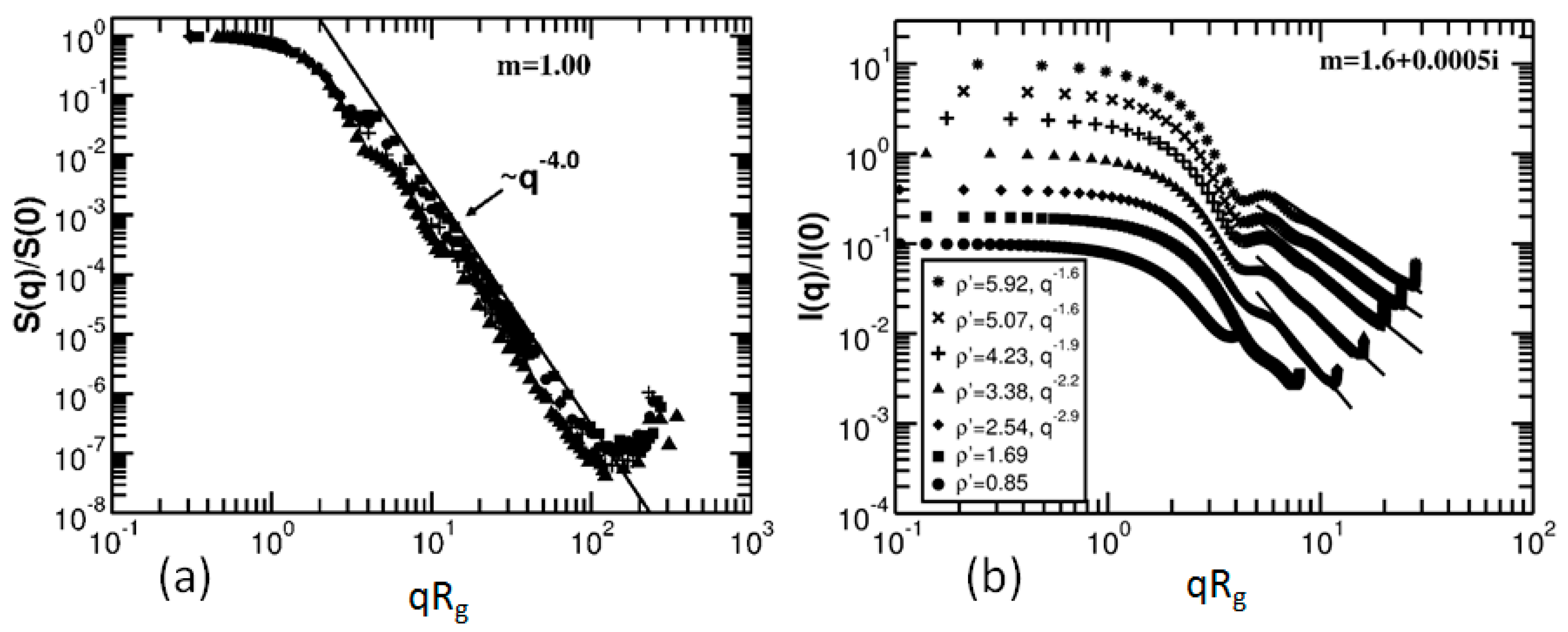
2. Q-Space Analysis Applied to Spheres
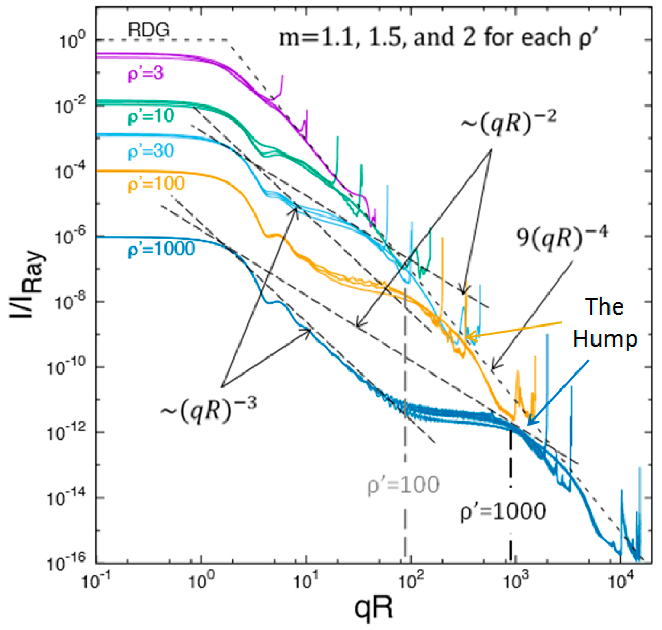
- For all , a forward scattering lobe of constant intensity appears when .
- With increasing qR, the scattering begins to decrease in the Guinier regime [9] near .
- After the Guinier regime, power law functionalities begin to appear. For , the RDG limit, a functionality follows the Guinier. When gets large, , a functionality (2d Fraunhofer diffraction [8], see below) appears after the Guinier regime.
- The regime is followed by a “hump” regime centered near qR which then crosses over to approximately touch the functionality of the RDG limit when .
- Connecting the Guinier regime and the hump regime with an equal tangent line gives a functionality which dominates, albeit briefly and imperfectly, when . We call the region between the Guinier regime and the backscattering the “power law regime”.
- At largest qR near 2kR (which corresponds to θ = 180°), enhanced backscattering occurs involving “rainbows” and the glory.
- 8.
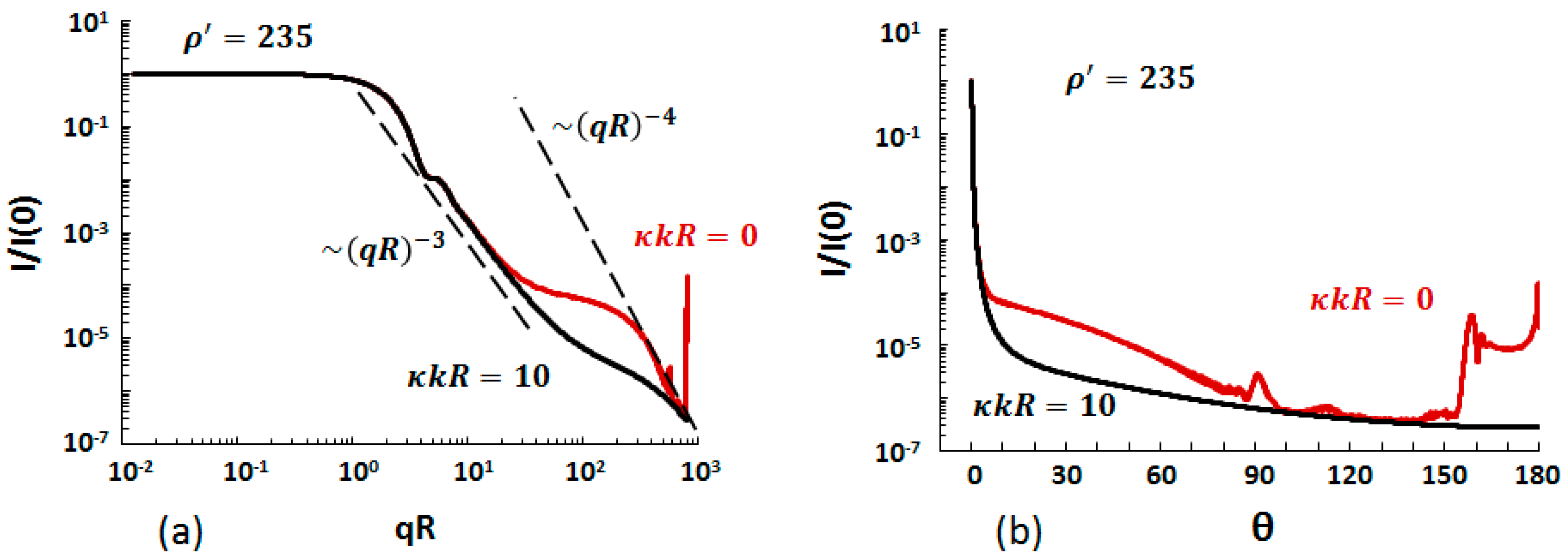
- When the refractive index, m = n + iκ, is complex, a second universal parameter comes into play, κkR. When κkR < 0.1, non-zero κ has very little effect on the scattering; otherwise κ does have an effect with the same effect for different kR and real part of the refractive index n if κkR is the same. The forward scattering when q < R−1 is not affected, but the hump and backscattering, including possible rainbows and glories incur substantial changes. For large size parameters, kR, disappearance of the hump correlates with the scattering cross section decreasing from approximately 2πR2 to πR2 and the absorption cross section increasing from 0 to πR2 when κkR ≥ 3 [13].
3. Experimental Data
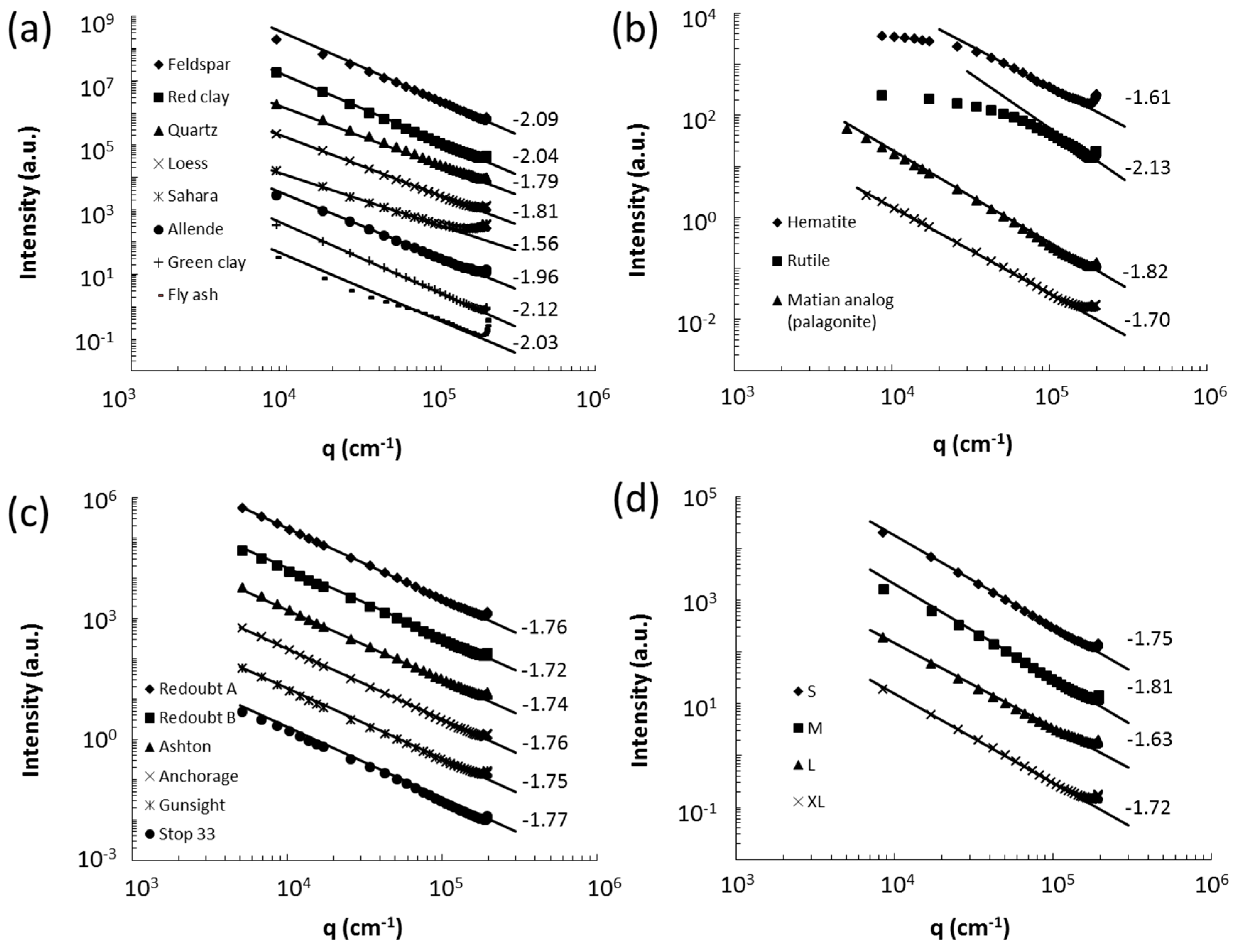
3.1. Dusts
3.1.1. Amsterdam-Granada Data Set
3.1.2. Arizona Road Dust
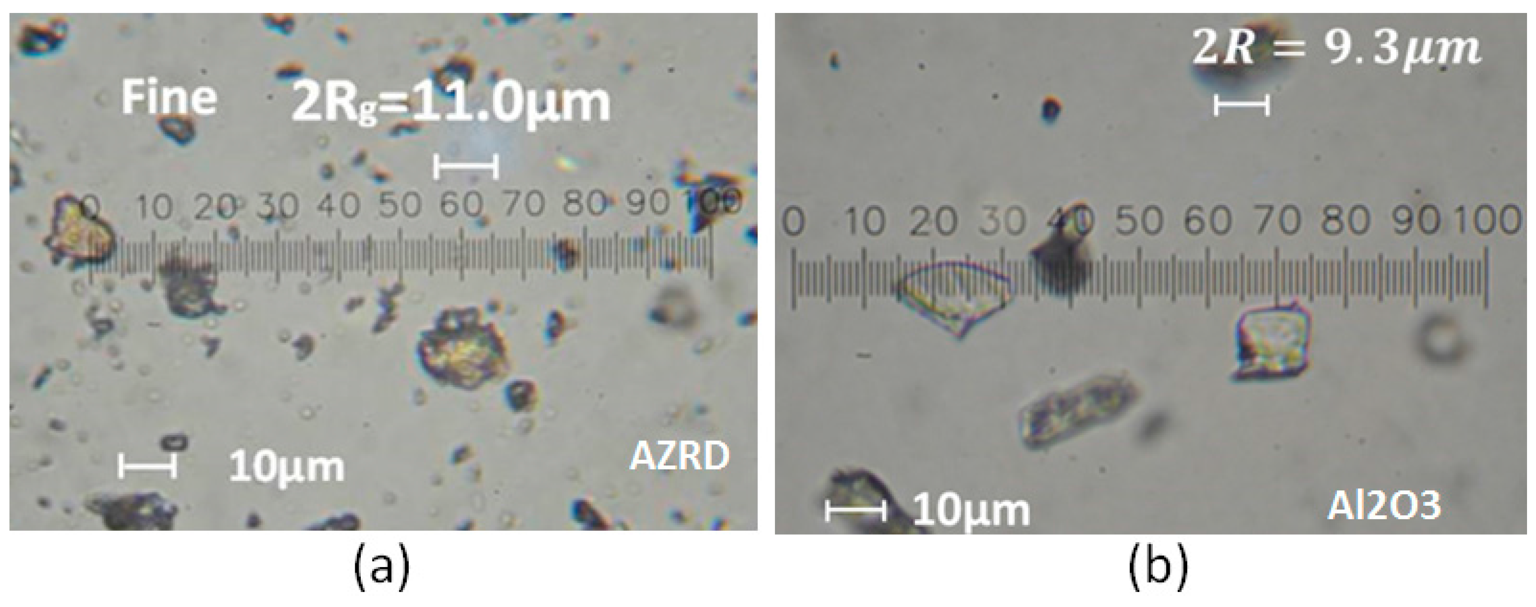
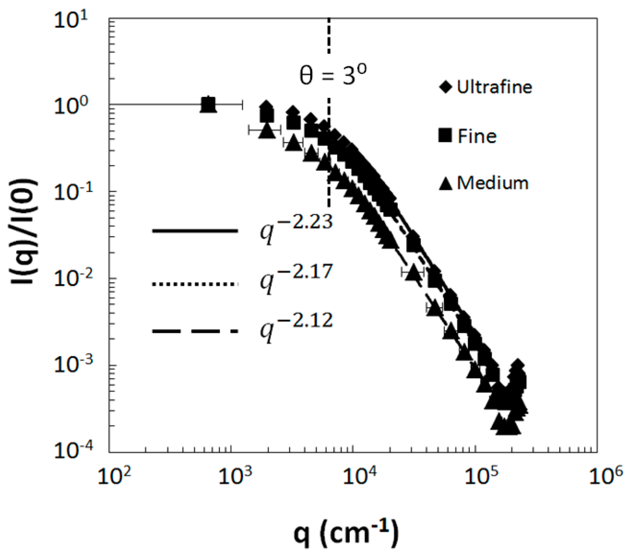
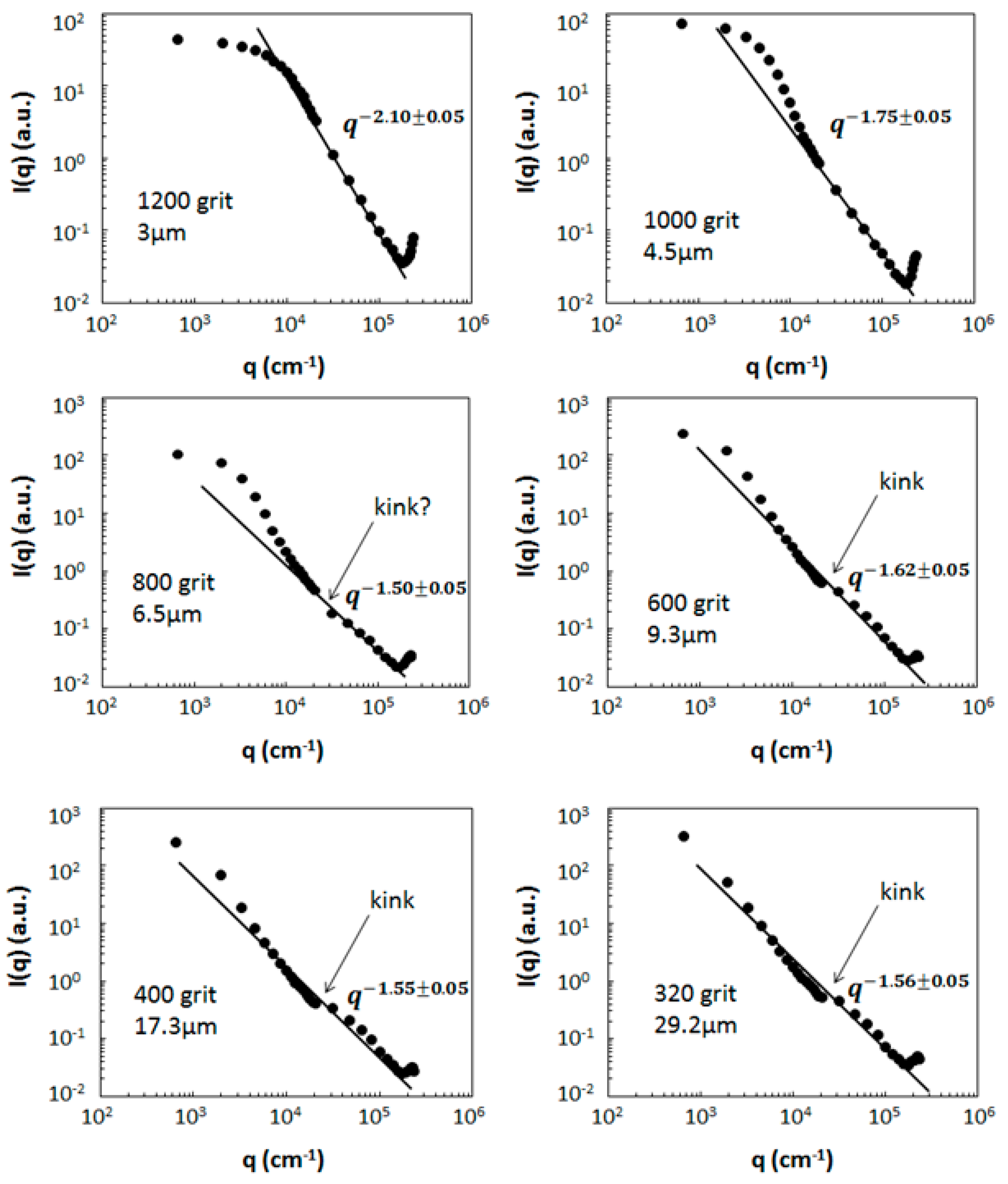
3.1.3. Al2O3 Abrasive Grits
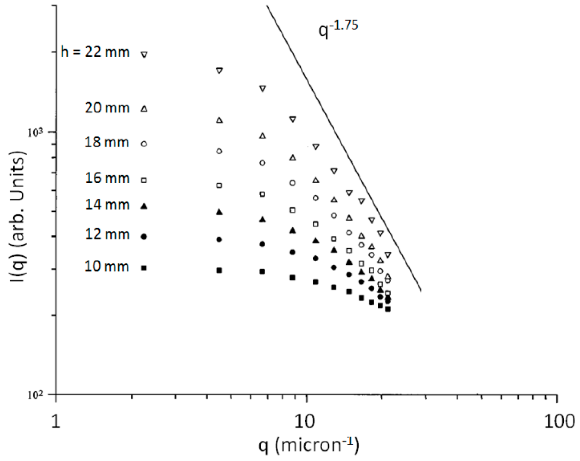
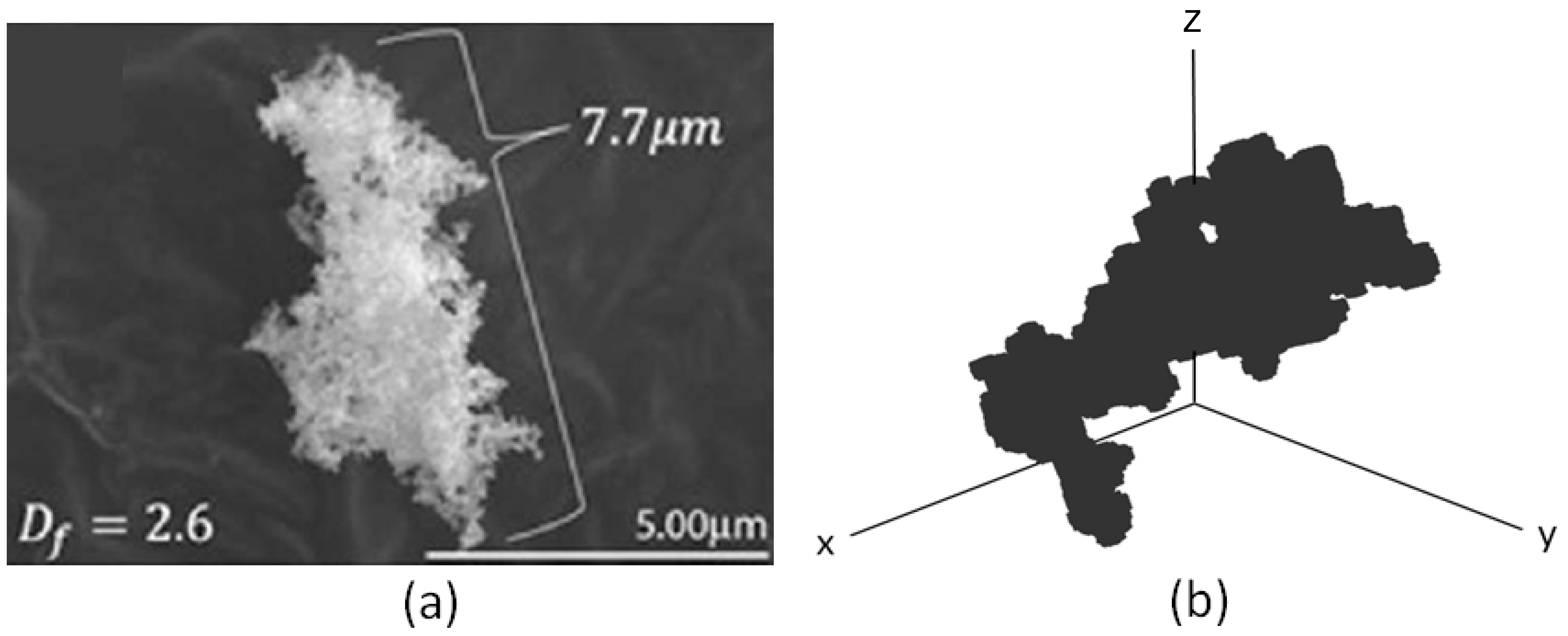
3.2. Fractal Aggregates
4. Theoretical Calculations
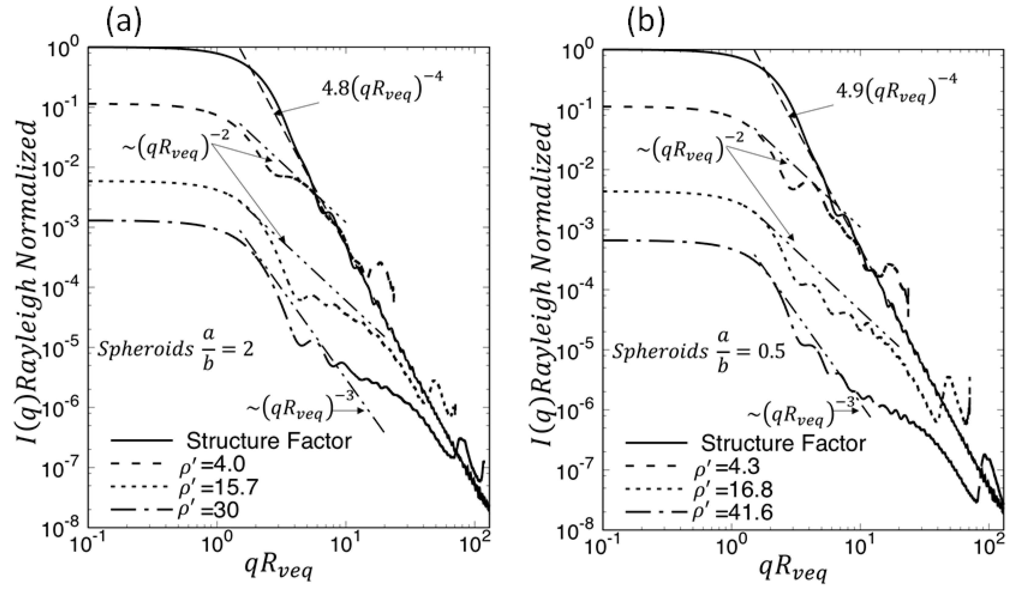
4.1. Spheroids
4.2. Irregular Spheres
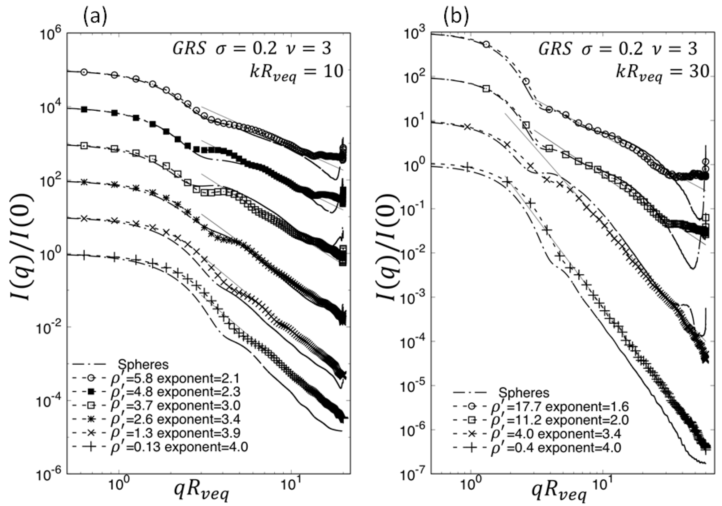
4.3. Gaussian Random Spheres
4.4. Thickened Clusters
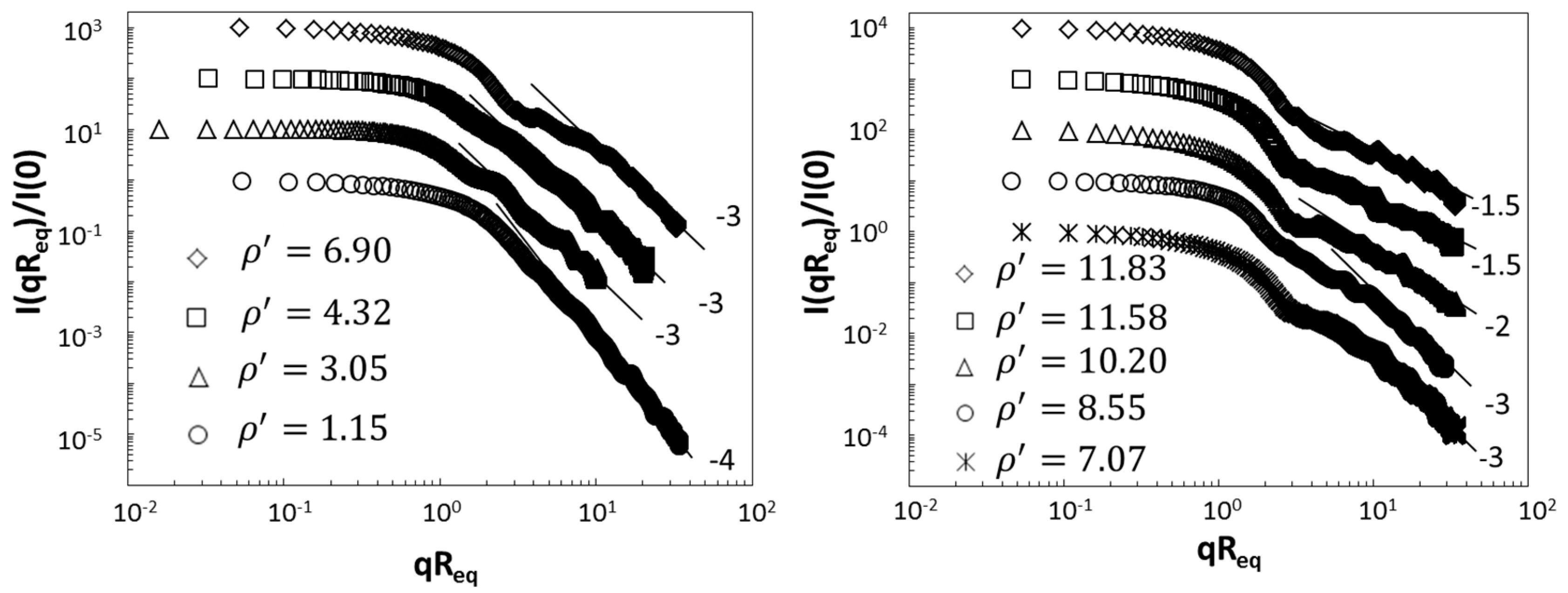
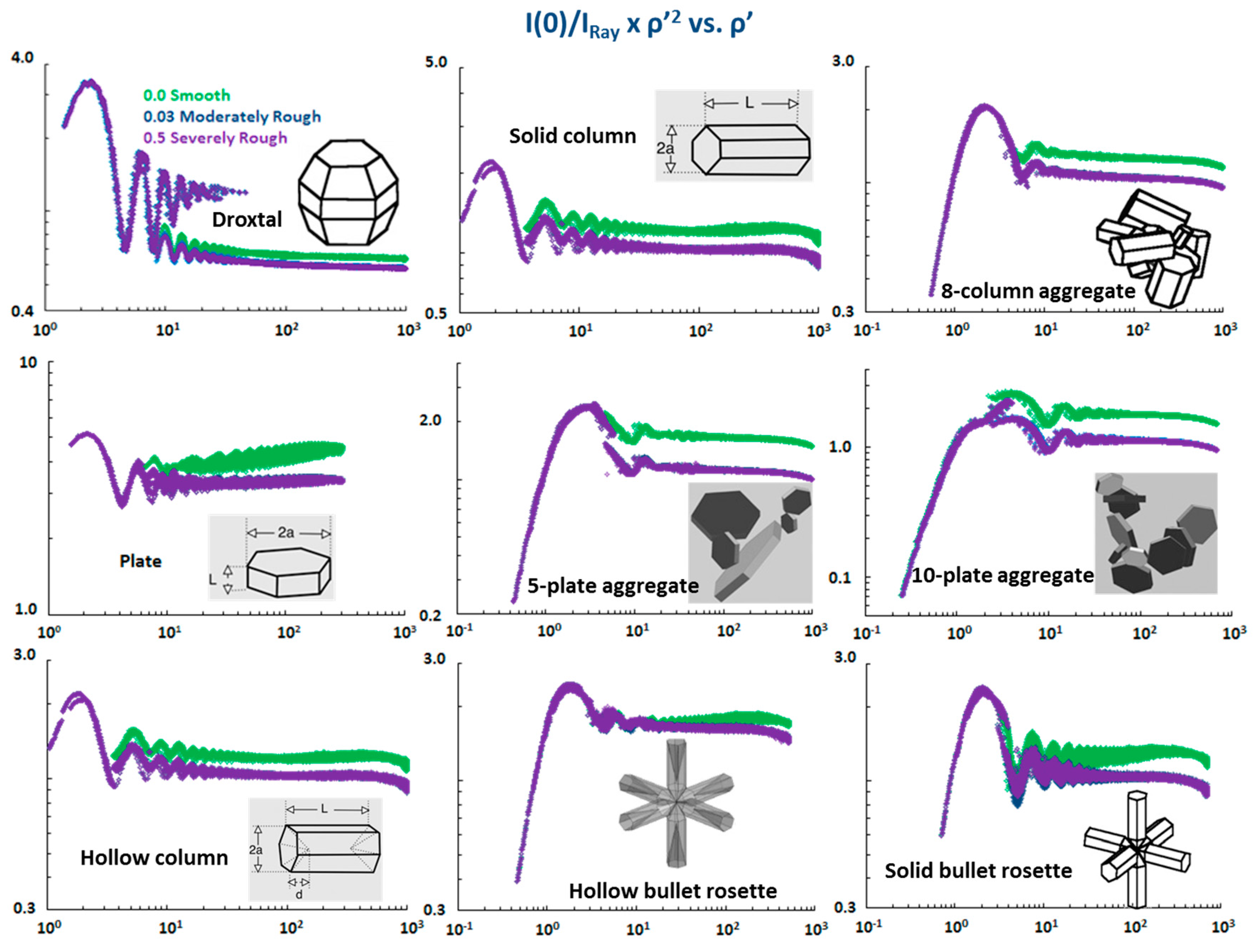
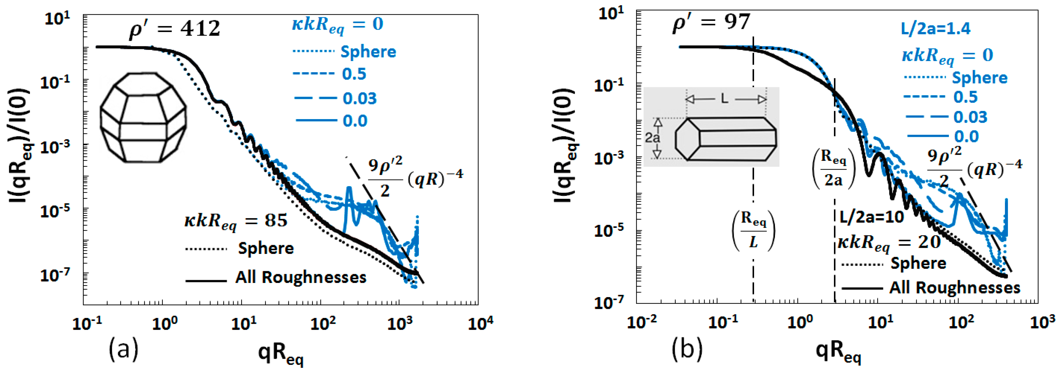
4.5. Ice Crystals
- The forward scattering lobe when behavior is very similar to that of spheres when the Rayleigh scattered intensity and internal coupling parameter are generalized for these shapes.
- Both spheres and ice crystals have a Guinier regime near . Unlike spheres, however, crystals with large aspect ratios can show two Guinier regimes.
- Both spheres and ice crystals have a complex power law regime beyond the Guinier regime when . This regime includes a (qReq)−3 functionality, for non-aggregate crystals, that starts to occur with large very likely due to 2d diffraction from the projected crystal shape. Similar to spheres, hump structure also appears centered near . At larger , there is a tendency to approach the spherical particle diffraction limit (RDG) of . Aggregate ice crystals have a more uniform power law regime similar to fractal aggregates.
- The parameter , plays the same role for both shapes by removing the hump near qReq ≃ .
- In many cases, the ice crystals have enhanced backscattering near , () similar but not the same as for spheres.
- The evolution of the scattering evolves away from the 3D diffraction with increasing for all shapes including spheres.
5. Discussion
- 1.
- A forward scattering lobe of constant intensity, i.e., q and θ independent, appears when . This condition is equivalent to θ < λ/2πR. The magnitude of the forward scattering is that of its generalized Rayleigh scattering, IRay, when ≤ 1, and IRay/2 when ≥ 10. We remark that for spheres approximately half of the total scattered light occurs when qR < π (θ < λ/2R) [6,13,49] and when κkR < 0.1, and nearly all the scattered light appears in this forward lobe when κkR > 10.
- 2.
- A Guinier regime near (θ ≈ λ/2πR).
- 3.
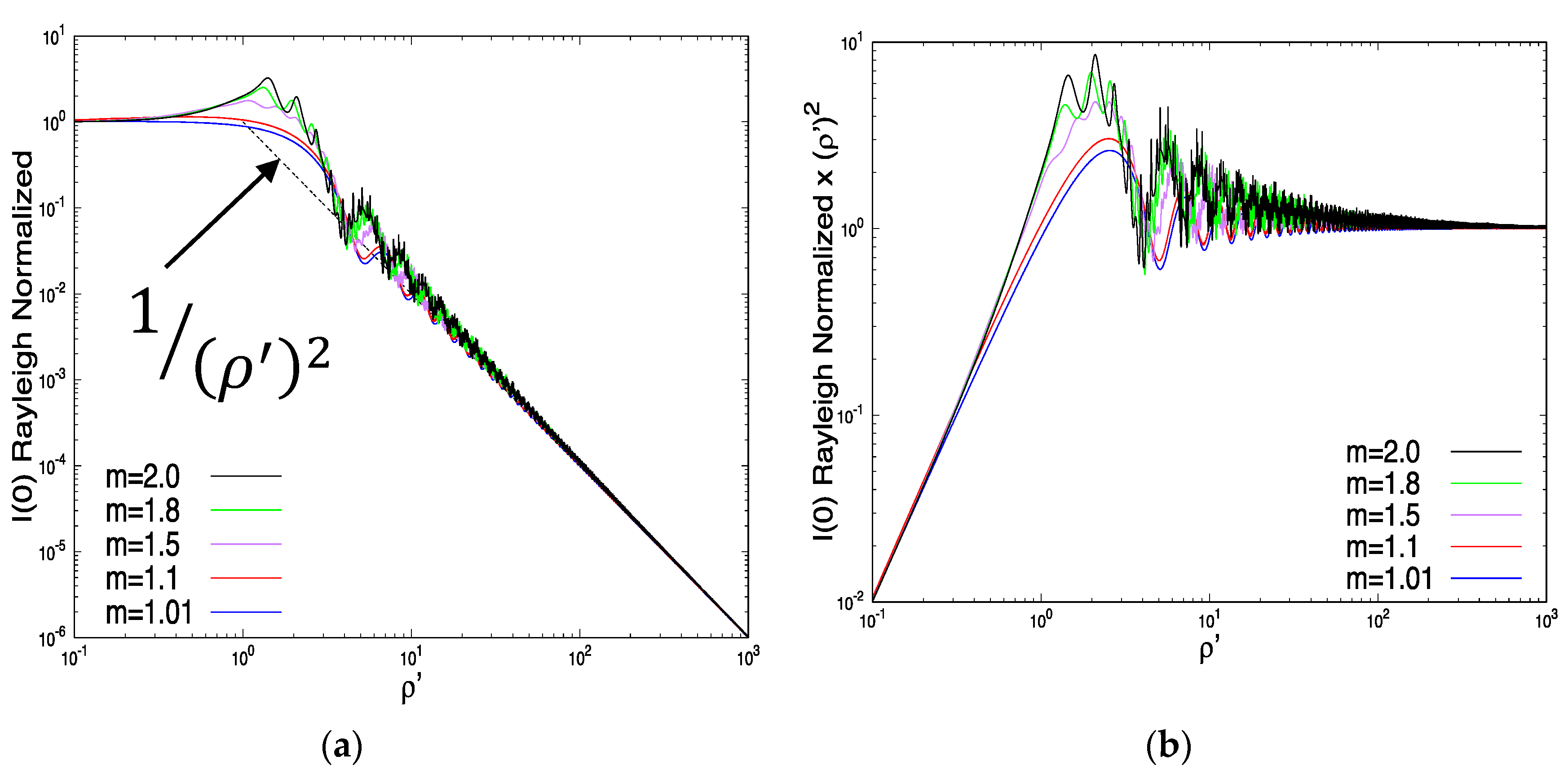
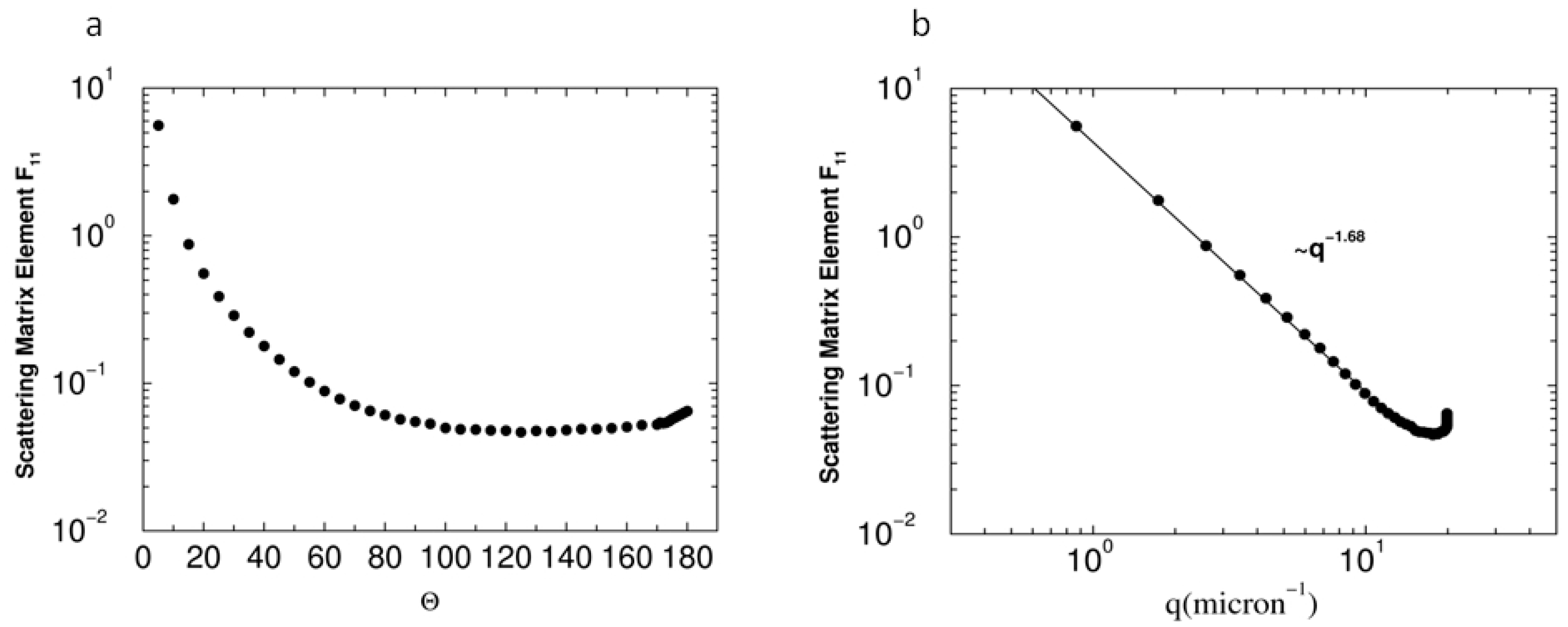
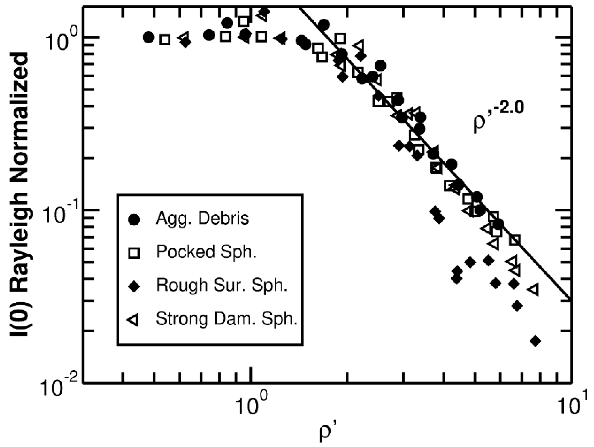
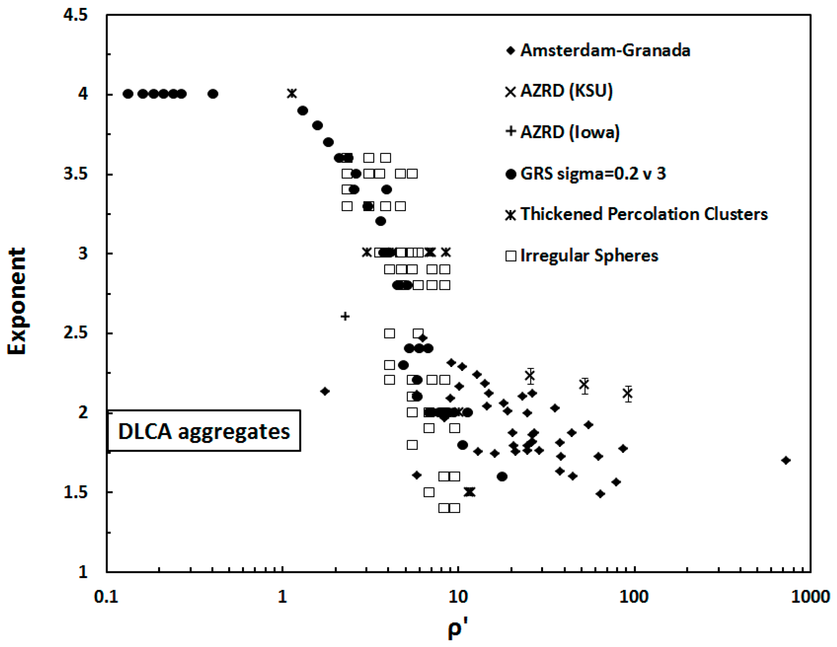
- A power law regime when 1 ≤ qR ≤ 1.5kR (λ/2πR ≤ θ ≤ 90 to 100°). This power law regime can be very complex as for spheres, spheroids, Gaussian random spheres and ice crystals, or it can be a single power law as for many of the dusts, fractal aggregates, irregular spheres, and thickened clusters. In all cases the power law regime evolves with the internal coupling parameter .
- 4.
- A dip near qR 3 to 4 (θ λ/2R) immediately after the Guinier regime appears for all shapes except the dusts and the DLCA aggregates. Recall that the dusts samples were polydisperse and this could smooth away any dip present in a single size scattering.
- 5.
- A (qR)−3 regime at large appears for spheres, spheroids and the non-aggregate ice crystals. This is due to the onset of 2d Fraunhofer diffraction, thus it is expected that all non-aggregate shapes would have this regime at .
- 6.
- A “hump” regime centered near qR when ≥ 30 for spheres, spheroids and, remarkably, ice crystals. This hump disappears when κkR ≥ 3. We expect this hump to appear as the 2D Fraunhofer diffraction, (qR)−3 regime appears at large for all shapes except aggregates.
- 7.
- An enhanced backscattering regime appears when qR ≥ 1.5 (θ ≥ 110°) for all shapes except the ice crystal aggregates, DLCA and thickened aggregates. A caveat is that the data for the DLCA aggregate was limited to θ ≤ 120°. The backscattering appears as increases there being no enhanced backscattering in the diffraction limit when = 0. Typically it appears when > 10.
6. Conclusions
Acknowledgments
Author Contributions
Conflicts of Interest
References
- Sorensen, C.M.; Fischbach, D.J. Patterns in Mie scattering. Opt. Commun. 2000, 173, 145–153. [Google Scholar] [CrossRef]
- Berg, M.J.; Sorensen, C.M.; Chakrabarti, A. Patterns in Mie scattering: Evolution when normalized by the rayleigh cross section. Appl. Opt. 2005, 44, 7487–7493. [Google Scholar] [CrossRef] [PubMed]
- Sorensen, C.M. Q-space analysis of scattering by particles: A review. J. Quant. Spectrosc. Radiat. 2013, 131, 3–12. [Google Scholar] [CrossRef]
- Van de Hulst, H.C. Light Scattering by Small Particles; Wiley: New York, NY, USA, 1957; p. 470. [Google Scholar]
- Kerker, M. The Scattering of Light, and Other Electromagnetic Radiation; Academic Press: New York, NY, USA, 1969; p. 666. [Google Scholar]
- Bohren, C.F.; Huffman, D.R. Absorption and Scattering of Light by Small Particles; Wiley: New York, NY, USA, 1983; p. 350. [Google Scholar]
- Heinson, W.R.; Chakrabarti, A.; Sorensen, C.M. A new parameter to describe light scattering by an arbitrary sphere. Opt. Commun. 2015, 356, 612–615. [Google Scholar] [CrossRef]
- Heinson, W.R.; Chakrabarti, A.; Sorensen, C.M. Crossover from spherical particle Mie scattering to circular aperture diffraction. J. Opt. Soc. Am. A 2014, 31, 2362–2364. [Google Scholar] [CrossRef] [PubMed]
- Guinier, A.; Fournet, G. Small-Angle Scattering of X-rays; Wiley: New York, NY, USA, 1955; p. 268. [Google Scholar]
- Heinson, Y.W.; Maughan, J.B.; Ding, J.C.; Chakrabarti, A.; Yang, P.; Sorensen, C.M. Q-space analysis of light scattering by ice crystals. J. Quant. Spectrosc. Radiat. 2016, 185, 86–94. [Google Scholar] [CrossRef]
- Hecht, E. Optics, 4th ed.; Addison-Wesley: Reading, MA, USA, 2002; p. 698. [Google Scholar]
- Wang, G.; Chakrabarti, A.; Sorensen, C.M. Effect of the imaginary part of the refractive index on light scattering by spheres. J. Opt. Soc. Am. A 2015, 32, 1231–1235. [Google Scholar] [CrossRef] [PubMed]
- Sorensen, C.M.; Maughan, J.B.; Chakrabarti, A. The partial light scattering cross section of spherical particles. J. Opt. Soc. Am. A. accepted for publication.
- Munoz, O.; Moreno, F.; Guirado, D.; Dabrowska, D.D.; Volten, H.; Hovenier, J.W. The amsterdam-granada light scattering database. J. Quant. Spectrosc. Radiat. 2012, 113, 565–574. [Google Scholar] [CrossRef]
- Munoz, O.; Volten, H.; Hovenier, J.W.; Nousiainen, T.; Muinonen, K.; Guirado, D.; Moreno, F.; Waters, L.B.F.M. Scattering matrix of large saharan dust particles: Experiments and computations. J. Geophys. Res. Atmos. 2007, 112. [Google Scholar] [CrossRef]
- Sorensen, C.M. Q-space analysis of scattering by dusts. J. Quant. Spectrosc. Radiat. 2013, 115, 93–95. [Google Scholar] [CrossRef]
- Heinson, Y.W.; Maughan, J.B.; Heinson, W.R.; Chakrabarti, A.; Sorensen, C.M. Light scattering q-space analysis of irregularly shaped particles. J. Geophys. Res. Atmos. 2016, 121, 682–691. [Google Scholar]
- Volten, H.; Munoz, O.; Rol, E.; de Haan, J.F.; Vassen, W.; Hovenier, J.W.; Muinonen, K.; Nousiainen, T. Scattering matrices of mineral aerosol particles at 441.6 nm and 632.8 nm. J. Geophys. Res. Atmos. 2001, 106, 17375–17401. [Google Scholar] [CrossRef]
- Munoz, O.; Volten, H.; de Haan, J.F.; Vassen, W.; Hovenier, J.W. Experimental determination of scattering matrices of olivine and allende meteorite particles. Astron. Astrophys. 2000, 360, 777–788. [Google Scholar]
- Munoz, O.; Volten, H.; de Haan, J.F.; Vassen, W.; Hovenier, J.W. Experimental determination of scattering matrices of randomly oriented fly ash and clay particles at 442 and 633 nm. J. Geophys. Res. Atmos. 2001, 106, 22833–22844. [Google Scholar] [CrossRef]
- Shkuratov, Y.; Ovcharenko, A.; Zubko, E.; Volten, H.; Munoz, O.; Videen, G. The negative polarization of light scattered from particulate surfaces and of independently scattering particles. J. Quant. Spectrosc. Radiat. 2004, 88, 267–284. [Google Scholar] [CrossRef]
- Munoz, O.; Volten, H.; Hovenier, J.W.; Min, M.; Shkuratov, Y.G.; Jalava, J.P.; van der Zande, W.J.; Waters, L.B.F.M. Experimental and computational study of light scattering by irregular particles with extreme refractive indices: Hematite and rutile. Astron. Astrophys. 2006, 446, 525–535. [Google Scholar] [CrossRef]
- Laan, E.C.; Volten, H.; Stam, D.M.; Munoz, O.; Hovenier, J.W.; Roush, T.L. Scattering matrices and expansion coefficients of martian analogue palagonite particles. Icarus 2009, 199, 219–230. [Google Scholar] [CrossRef][Green Version]
- Munoz, O.; Volten, H.; Hovenier, J.W.; Veihelmann, B.; van der Zande, W.J.; Waters, L.B.F.M.; Rose, W.I. Scattering matrices of volcanic ash particles of Mount ST. Helens, Redoubt, and Mount Spurr volcanoes. J. Geophys. Res. Atmos. 2004, 109. [Google Scholar] [CrossRef]
- Wang, Y.; Chakrabarti, A.; Sorensen, C.M. A light-scattering study of the scattering matrix elements of arizona road dust. J. Quant. Spectrosc. Radiat. 2015, 163, 72–79. [Google Scholar] [CrossRef]
- Heinson, Y.W.; Chakrabarti, A.; Sorensen, C.M. A light-scattering study of Al2O3 abrasives of various grit sizes. J. Quant. Spectrosc. Radiat. 2016, 180, 84–91. [Google Scholar] [CrossRef]
- Sorensen, C.M. Light scattering by fractal aggregates: A review. Aerosol Sci. Technol. 2001, 35, 648–687. [Google Scholar] [CrossRef]
- Sorensen, C.M.; Oh, C.; Schmidt, P.W.; Rieker, T.P. Scaling description of the structure factor of fractal soot composites. Phys. Rev. E 1998, 58, 4666–4672. [Google Scholar] [CrossRef]
- Dubovik, O.; Sinyuk, A.; Lapyonok, T.; Holben, B.N.; Mishchenko, M.; Yang, P.; Eck, T.F.; Volten, H.; Munoz, O.; Veihelmann, B.; et al. Application of spheroid models to account for aerosol particle nonsphericity in remote sensing of desert dust. J. Geophys. Res. Atmos. 2006, 111. [Google Scholar] [CrossRef]
- Mishchenko, M.I.; Travis, L.D. Capabilities and limitations of a current FORTRAN implementation of the T-matrix method for randomly oriented, rotationally symmetric scatterers. J. Quant. Spectrosc. Radiat. 1998, 60, 309–324. [Google Scholar] [CrossRef]
- Mishchenko, M.I.; Travis, L.D.; Mackowski, D.W. T-matrix computations of light scatteringby nonspherical particles: A review. J. Quant. Spectrosc. Radiat. 2010, 111, 1704–1744. [Google Scholar]
- Maughan, J.B.; Chakrabarti, A.; Sorensen, C.M. Rayleigh scattering and the internal coupling parameter for arbitrary shapes. J. Quant. Spectrosc. Radiat. 2017, 189, 339–343. [Google Scholar]
- Yurkin, M.A.; Hoekstra, A.G. The discrete dipole approximation: An overview and recent developments. J. Quant. Spectrosc. Radiat. 2007, 106, 558–589. [Google Scholar] [CrossRef]
- Sorensen, C.M.; Zubko, E.; Heinson, W.R.; Chakrabarti, A. Q-space analysis of scattering by small irregular particles. J. Quant. Spectrosc. Radiat. 2014, 133, 99–105. [Google Scholar] [CrossRef][Green Version]
- Zubko, E.; Shkuratov, Y.; Kiselev, N.N.; Videen, G. Dda simulations of light scattering by small irregular particles with various structure. J. Quant. Spectrosc. Radiat. 2006, 101, 416–434. [Google Scholar] [CrossRef]
- Zubko, E.; Shkuratov, Y.; Mishchenko, M.; Videen, G. Light scattering in a finite multi-particle system. J. Quant. Spectrosc. Radiat. 2008, 109, 2195–2206. [Google Scholar] [CrossRef]
- Zubko, E.; Kimura, H.; Shkuratov, Y.; Muinonen, K.; Yamamoto, T.; Okamoto, H.; Videen, G. Effect of absorption on light scattering by agglomerated debris particles. J. Quant. Spectrosc. Radiat. 2009, 110, 1741–1749. [Google Scholar]
- Purcell, E.M.; Pennypacker, C.R. Scattering and absorption of light by nonspherical dielectric grains. Astrophys. J. 1973, 186, 705–714. [Google Scholar] [CrossRef]
- Yurkin, M.A.; Maltsev, V.P.; Hoekstra, A.G. The discrete dipole approximation for simulation of light scattering by particles much larger than the wavelength. J. Quant. Spectrosc. Radiat. 2007, 106, 546–557. [Google Scholar]
- Yurkin, M.A.; Hoekstra, A.G. The discrete-dipole-approximation code ADDA: Capabilities and known limitations. J. Quant. Spectrosc. Radiat. 2011, 112, 2234–2247. [Google Scholar] [CrossRef]
- Oh, C.; Sorensen, C.M. Scaling approach for the structure factor of a generalized system of scatterers. J. Nanopart Res. 1999, 1, 369–377. [Google Scholar] [CrossRef]
- Muinonen, K.; Zubko, E.; Tyynela, J.; Shkuratov, Y.G.; Videen, G. Light scattering by gaussian random particles with discrete-dipole approximation. J. Quant. Spectrosc. Radiat. 2007, 106, 360–377. [Google Scholar] [CrossRef]
- Maughan, J.B.; Sorensen, C.M.; Chakrabarti, A. Q-space analysis of light scattering by gaussian random spheres. J. Quant. Spectrosc. Radiat. 2016, 174, 14–21. [Google Scholar] [CrossRef]
- Chakrabarty, R.K.; Beres, N.D.; Moosmuller, H.; China, S.; Mazzoleni, C.; Dubey, M.K.; Liu, L.; Mishchenko, M.I. Soot superaggregates from flaming wildfires and their direct radiative forcing. Sci. Rep. UK 2014, 4, 5508. [Google Scholar] [CrossRef] [PubMed]
- Berg, M.J.; Sorensen, C.M. Internal fields of soot fractal aggregates. J. Opt. Soc. Am. A 2013, 30, 1947–1955. [Google Scholar]
- Zubko, E.; Petrov, D.; Grynko, Y.; Shkuratov, Y.; Okamoto, H.; Muinonen, K.; Nousiainen, T.; Kimura, H.; Yamamoto, T.; Videen, G. Validity criteria of the discrete dipole approximation. Appl. Opt. 2010, 49, 1267–1279. [Google Scholar] [CrossRef] [PubMed]
- Yurkin, M.A.; de Kanter, D.; Hoekstra, A.G. Accuracy of the discrete dipole approximation for simulation of optical properties of gold nanoparticles. J. Nanophoton. 2010, 4, 041585. [Google Scholar]
- Yang, P.; Bi, L.; Baum, B.A.; Liou, K.N.; Kattawar, G.W.; Mishchenko, M.I.; Cole, B. Spectrally consistent scattering, absorption, and polarization properties of atmospheric ice crystals at wavelengths from 0.2 to 100 µm. J. Atmos. Sci. 2013, 70, 330–347. [Google Scholar]
- Brillouin, L. The scattering cross section of spheres for electromagnetic waves. J. Appl. Phys. 1949, 20, 1110–1125. [Google Scholar] [CrossRef]
- Curtis, D.B.; Meland, B.; Aycibin, M.; Arnold, N.P.; Grassian, V.H.; Young, M.A.; Kleiber, P.D. A laboratory investigation of light scattering from representative components of mineral dust aerosol at a wavelength of 550 nm. J. Geophys. Res. Atmos. 2008, 113, 693–702. [Google Scholar] [CrossRef]


© 2017 by the authors. Licensee MDPI, Basel, Switzerland. This article is an open access article distributed under the terms and conditions of the Creative Commons Attribution (CC BY) license (http://creativecommons.org/licenses/by/4.0/).
Share and Cite
Sorensen, C.M.; Heinson, Y.W.; Heinson, W.R.; Maughan, J.B.; Chakrabarti, A. Q-Space Analysis of the Light Scattering Phase Function of Particles with Any Shape. Atmosphere 2017, 8, 68. https://doi.org/10.3390/atmos8040068
Sorensen CM, Heinson YW, Heinson WR, Maughan JB, Chakrabarti A. Q-Space Analysis of the Light Scattering Phase Function of Particles with Any Shape. Atmosphere. 2017; 8(4):68. https://doi.org/10.3390/atmos8040068
Chicago/Turabian StyleSorensen, Christopher M., Yuli W. Heinson, William R. Heinson, Justin B. Maughan, and Amit Chakrabarti. 2017. "Q-Space Analysis of the Light Scattering Phase Function of Particles with Any Shape" Atmosphere 8, no. 4: 68. https://doi.org/10.3390/atmos8040068
APA StyleSorensen, C. M., Heinson, Y. W., Heinson, W. R., Maughan, J. B., & Chakrabarti, A. (2017). Q-Space Analysis of the Light Scattering Phase Function of Particles with Any Shape. Atmosphere, 8(4), 68. https://doi.org/10.3390/atmos8040068