All articles published by MDPI are made immediately available worldwide under an open access license. No special
permission is required to reuse all or part of the article published by MDPI, including figures and tables. For
articles published under an open access Creative Common CC BY license, any part of the article may be reused without
permission provided that the original article is clearly cited. For more information, please refer to
https://www.mdpi.com/openaccess.
Feature papers represent the most advanced research with significant potential for high impact in the field. A Feature
Paper should be a substantial original Article that involves several techniques or approaches, provides an outlook for
future research directions and describes possible research applications.
Feature papers are submitted upon individual invitation or recommendation by the scientific editors and must receive
positive feedback from the reviewers.
Editor’s Choice articles are based on recommendations by the scientific editors of MDPI journals from around the world.
Editors select a small number of articles recently published in the journal that they believe will be particularly
interesting to readers, or important in the respective research area. The aim is to provide a snapshot of some of the
most exciting work published in the various research areas of the journal.
We suggest a conceptual approach for measuring the near-surface wind vector over water using the airborne weather radar, in addition to its standard meteorological and navigation applications. The airborne weather radar operates in the ground-mapping mode in the range of high to medium incidence angles as a scatterometer. Using the aircraft rectilinear flight over the water surface, measuring the geometry and the geophysical model function, we show that the wind vector can be successfully recovered from the azimuth normalized radar cross-section data obtained from a scanning sector of up to ±100°. The efficiency and accuracy of the proposed wind vector measurement algorithms are supported by computer simulations indicating their potential as a powerful tool for the wind field reconstruction. Some limitations and recommendations of the suggested approach are further discussed.
The oceans interact with the atmosphere to control and regulate the environment on Earth. Fed by the sun, the interactions between the land, ocean, and atmosphere produce the phenomena of weather and climate. Information on surface wind vector and wave height is assimilated into regional and global numerical weather and wave models, thereby extending and improving our ability to predict future weather patterns and sea surface conditions [1].
During the last half-century, meteorologists have begun to understand weather patterns well enough to produce sufficiently accurate forecasts of future weather patterns. At first, only local oceanic weather conditions were available from sparsely arrayed weather stations, ships, and oceans buoys. Later on, satellite and airborne remote sensing has improved the situation significantly. Satellite remote sensing has demonstrated its potential to provide measurements of weather conditions on a global scale while airborne remote sensing found similar applications on a local scale.
Wind and wave measuring systems can be classified into the following two categories [2]:
(1)
operational systems, providing continuous, global, or regional observations for forecasting, data assimilation, and model validation;
(2)
systems operating with higher temporal and spatial resolution during limited measurement campaigns in order to study the physical processes of wave generation and air/sea interaction.
The near-surface wind measurements over sea are very important for meteorology, as well as for navigation and operational oceanography.
On the global scale, the information about sea winds and waves, in general, can be obtained from a satellite using active microwave instruments, namely a scatterometer, Synthetic Aperture Radar (SAR), and a radar altimeter. However, for local numerical weather and wave models, the local data on wave height and wind speed and direction are required.
Wind and wave measuring by these remote sensing instruments is based on the features of microwave backscattering from the water surface. Scatterometers provide estimates of the near-surface wind vector because the normalized radar cross section (NRCS) of the water surface depends on the wind speed and direction. The accuracy of the wind direction measurement is ±20°, and the accuracy of the wind speed measurement is ±2 m/s in the wind speed range of 3–24 m/s.
In order to retrieve the wind vector from NRCS measurements, the relationship between the NRCS and near-surface wind, called the “geophysical model function,” is applied. Scatterometer experiments have shown that the NRCS model function for medium incidence angles at the appropriate transmitted and received polarization (vertical or horizontal) can be represented by one of the widely used forms such as [3]
where subscripts pp represent the transmitted and received polarization (V—vertical, H—horizontal); , , and are the Fourier terms that depend on sea surface wind speed and incidence angle, , , and ; , , , , , and are the coefficients dependent on the incidence angle.
NRCS azimuth curve Equation (1) has two maxima and two minima. The principal maximum is located in the up-wind direction, the second maximum corresponds to the down-wind direction, and the two minima are in the cross-wind directions displaced slightly in the second maximum direction. With the increase of the incidence angle, the difference between the two maxima and the difference between the maxima and minima becomes so significant (especially at medium incidence angles) that this feature can be used for the retrieval of the wind direction over water [4].
Generally, the problem of estimating the navigational direction of the sea surface wind ψw consists in defining the principal maximum of a curve of the reflected signal intensity (azimuth of the principal maximum of the NRCS curve ),
while the problem of deriving the sea surface wind speed consists in the determination of a reflected signal intensity value from the up-wind direction or from some or all of the azimuth directions.
Airborne scatterometer wind measurements are typically performed at either the circle track flight for a scatterometer with an inclined one-beam fixed-position antenna or the rectilinear track flight for a scatterometer with a rotating antenna [5,6,7]. Unfortunately, a microwave narrow-beam antenna has considerable size at Ku-, X- and C-bands that makes placing it on an aircraft difficult. Therefore, use of the modified conventional navigation instruments of aircraft in a scatterometer mode seems to be the best way in that case.
From that point of view, a promising navigation instrument is the airborne weather radar (AWR). In this connection, a conceptual approach for a rectilinear track flight measuring the wind vector over sea by the AWR having a wide-size scanning sector and operating in the ground-mapping mode as a scatterometer, in addition to its standard application, is discussed in this paper.
2. Materials and Methods
2.1. Airborne Weather Radar Functions and Applications
AWR is the radar equipment mounted on an aircraft for the purposes of weather observation and avoidance, finding the aircraft position relative to landmarks, and drift angle measurement [8]. The AWR is a required part of equipment and thus must be installed on all civil airliners. Military transport aircrafts are also usually equipped with weather radars. Due to the specificity of airborne applications, designers of avionics systems always try to use the most efficient progressive methods and reliable engineering solutions that provide flight safety and flight regularity in harsh environments [9].
AWR development is mainly associated with greater functionality in the detection of different dangerous weather phenomena. The radar observations involved in a weather mode are the magnitude detection of the reflections from clouds and precipitation, and Doppler measurements of the motion of particles within a weather formation. Magnitude detection allows for the determination of particle type (rain, snow, hail, etc.) and precipitation rate. Doppler measurements can be performed to yield estimates of turbulence intensity and wind speed. Reliable determination of the presence and severity of the phenomena, such as wind shear and microburst, are also important application areas of weather radars [10].
The second assignment of the AWR is providing a pilot with reliable navigation information using surface mapping. In this case, the possibility of extracting navigation information that allows for the determination of the aircraft position with respect to a geographic map is very important for air navigation. A landmark’s coordinates measured by the AWR relative to an aircraft make it possible to set a flight computer for a more exact and efficient en-route flight, cargo delivery, and cargo throw-down to a given point. Altogether, this improves tactical possibilities of transport aircrafts, airplanes for search-and-rescue services, and local airways [9]. Other specific functions of the AWR is the interaction with ground-based responder beacons. New functions of the AWR include the detection and visualization of runways at landing approaches, as well as the visualization of taxi routes and obstacles on said taxi routes during taxiing.
Certainly, not all of the mentioned functions are implemented in every particular airborne radar system. Nevertheless, the AWR is a multifunctional system that provides the possibility of Earth surface surveillance and weather observation. Usually, weather radar should at least be able to detect clouds and precipitation, select zones of meteorological danger, and show radar images of the underlying surface in the ground-mapping mode.
AWRs or multimode radars with a weather mode are usually nose-mounted. Most AWRs operate in either X- or C-band [10]. Newer radars operate in the X-band to maximize the radar reflectivity of weather formations, which is proportional to λ−4, where λ is the radar wavelength. At the same time, the long-range weather mode is provided in the X-band much more effectively than in the Ku-band. In the ground-mapping mode, the AWR antenna has a wide cosecant-squared elevation beam. A horizontal dimension of the beam is narrow (2° to 6°), while the vertical dimension is relatively wide (10° to 30°). The beam sweeps in an azimuth sector (up to ±100°) [8,9,10]. The scan plane is horizontal because the antenna is stabilized (roll-and-pitch-stabilized). Those AWR features enhance its functionality for its use in the ground-mapping mode as a scatterometer for measuring the water surface backscattering signature and the wind vector over the water surface.
2.2. Wind Vector Retrieval
Depending on the AWR scanning features, three general cases may take place: a narrow scanning sector, a medium scanning sector, and a wide scanning sector (±90° or wider, up to ±100°). The latter case allows obtaining azimuth NRCS values from a sector of up to 200° width. NRCS values are sampled from significantly different azimuth directions that provide sufficient information for wind vector estimation; thus, such an AWR seems to be the most suitable for measuring the wind speed and direction over water during a rectilinear flight.
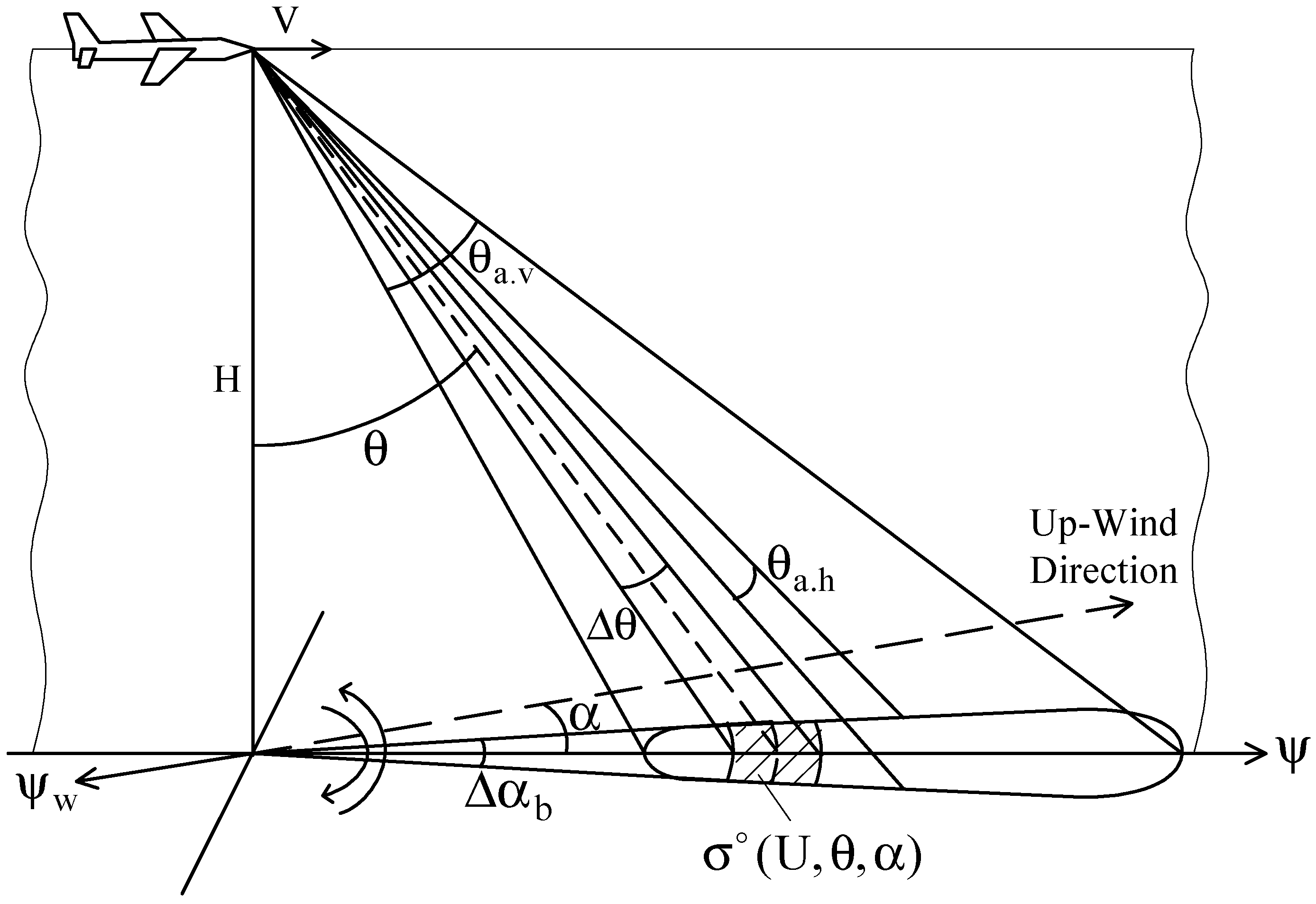
Let an aircraft equipped with an AWR make a horizontal rectilinear flight with the speed V at some altitude H above the mean sea surface. Let the AWR operate in the ground-mapping mode as a scatterometer, with the radar antenna having different beam width in the vertical θa.v and horizontal θa.h planes (), as shown in Figure 1, periodically scan through an azimuth in a sector wider than ±90°, and let a delay selection be used to provide a necessary resolution in the vertical plane. Then, the beam scanning allows for the selection of a power backscattered by the underlying surface for a given incidence angle θ from various directions in a wide azimuth sector. Angular selection (by a narrow horizontal beamwidth) in the horizontal plane along with the delay selection provides angular resolutions in the azimuthal and vertical planes, Δαb and Δθ, respectively.
Let the sea surface wind blow in direction ψw, and the angle between the up-wind direction and the aircraft course ψ be α. Furthermore, let the NRCS model function for medium incidence angles follow Equation (1). Since the selected cell is narrow enough in the vertical plane, the NRCS model function for medium incidence angles Equation (1) can be used without any correction in the wind measurement when the azimuth angular size of a cell is up to 15°–20° [11].
Angular resolution in the azimuthal plane is described as
Thus, from Equation (3), the AWR beam with a 2° beamwidth in the horizontal plane provides angular resolutions in the azimuthal plane of 2.8°, 2.6°, and 2.3° at incidence angles of 45°, 50°, and 60°, respectively. Alternatively, the AWR beam with a beamwidth of 6° in the same plane would provide azimuthal resolutions of 8.5°, 7.8°, and 6.9°, respectively, which are also rather suitable for airborne scatterometer wind measurement.
As AWR beam scans periodically through an azimuth, the current NRCS value is obtained not from the same direction but from a narrow sector having the azimuth width of Δαs. NRCS samples obtained from the narrow sector and averaged over all measured values in that sector provide an appropriate NRCS value corresponding to the azimuth angle of the sector. The number of narrow sectors formed in the wide scanning sector equals . Thus, N NRCS values can be obtained from significantly different azimuth angles, and a system of N equations from Equation (1) can be written.
Let a narrow sector width be 5°. Then, the number of the narrow sectors is 37, and the following system of 37 equations can be written:
where , …, , …, and are the NRCS values obtained from the directions , …, α, …, and , respectively.
Next, to retrieve the wind speed and up-wind direction from the azimuth NRCS data set obtained, the system of Equation (4) should be solved approximately using a searching procedure within the ranges of discrete values of possible solutions. Finally, the navigation wind direction can be found as
3. Results and Discussion
As shown above, the AWR operating in a wide-size scanning sector and employed in the ground-mapping mode as a scatterometer can be used for remotely measuring the near-surface wind vector over water by the analysis of the azimuth NRCS data, in addition to its typical meteorological and navigation application.
The AWR wide scanning sector concept is much more preferable in comparison with the medium sector [12] and especially the narrow sector [13], as it allows one to obtain NRCS values from significantly different azimuth directions that provide more accurate wind vector estimation. Despite the fact that the AWR during rectilinear flight measurement cannot be used to obtain an entire 360° azimuth NRSC data set, as it can during a classical circular flight or during a two-stage rectilinear flight [14], the rectilinear flight measurement is much faster and convenient for a pilot at operational measurements or other special missions.
Wind measurement is started when a stable horizontal rectilinear flight at a given altitude and the speed of flight has been established. The measurement is finished when the required number of NRCS samples for each narrow azimuth sector observed is obtained. To obtain a greater number of NRCS samples for each direction observed, several consecutive beam sweeps should be used.
Based on the data processing, two wind estimation modes can be realized for AWR: a normal mode and a fast mode. In the normal mode, all the NRCS data obtained for directions , …, α, …, and are used, and the wind retrieval performs with the system of Equation (4). Processing can be sped up by narrowing the range of possible wind speeds. A lower wind speed UL and an upper wind speed UU can be found using an averaged 180° azimuth NRSC value from the following equations:
and
The fast mode uses only five NRCSs obtained for directions , , α, , and . For this mode, a system of equations contains only five equations for , , , , and [13]. The wind speed can be found from the following equation:
taking into account that:
Then, two possible up-wind directions relative to the aircraft course can be found.
The unique up-wind direction α relative to the aircraft course can be found by substitution of the values α1 and α2 into equations for and of the system of equations. Finally, the wind direction can be retrieved from Equation (5).
In principle, the fast mode results can be used as first-order estimates for further, more precise calculations of the wind speed and direction in the normal mode.
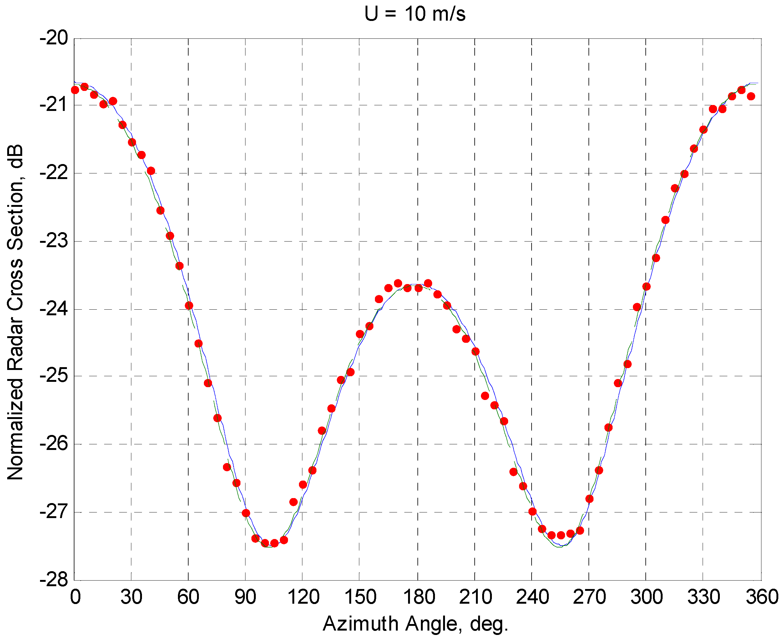
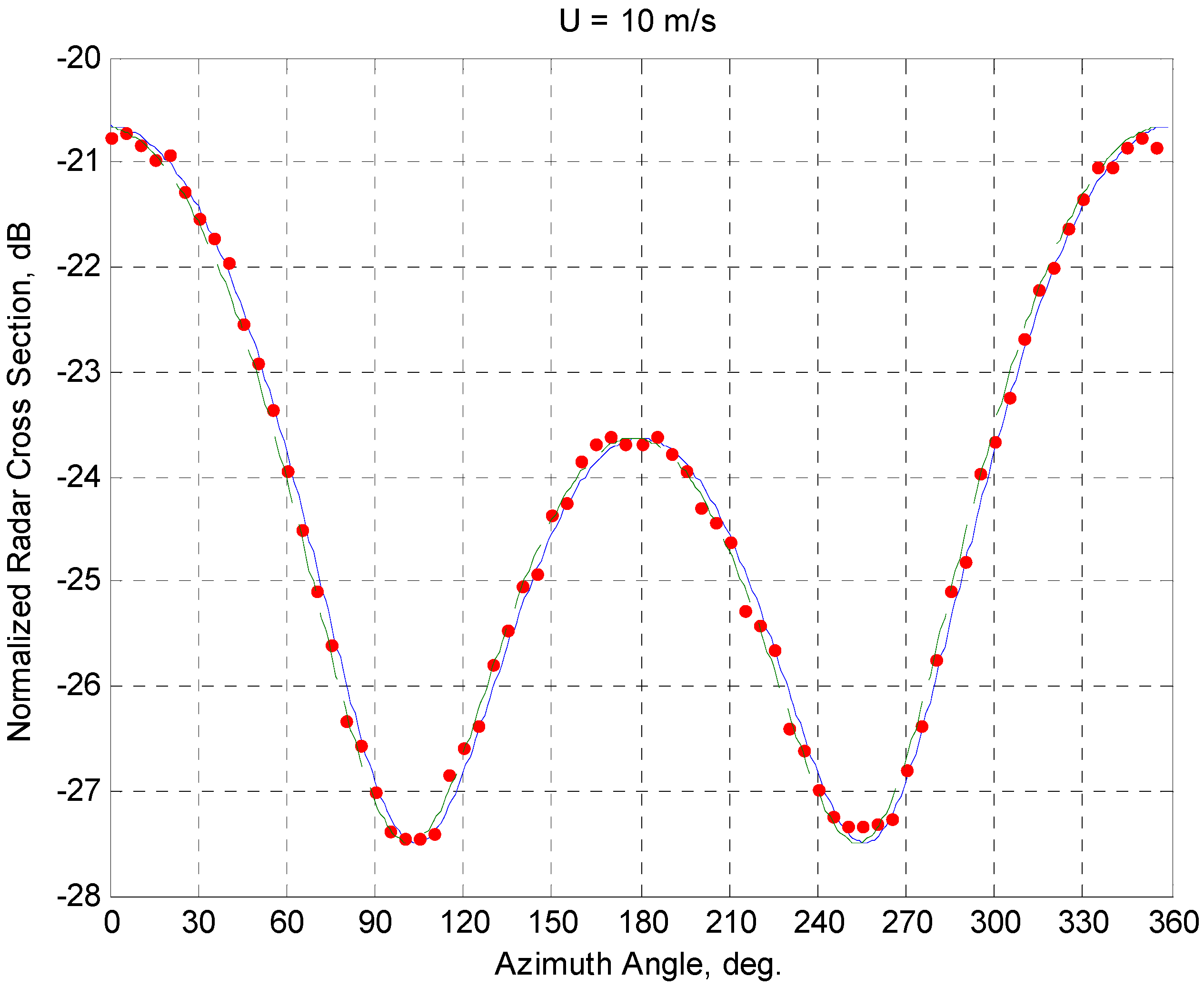
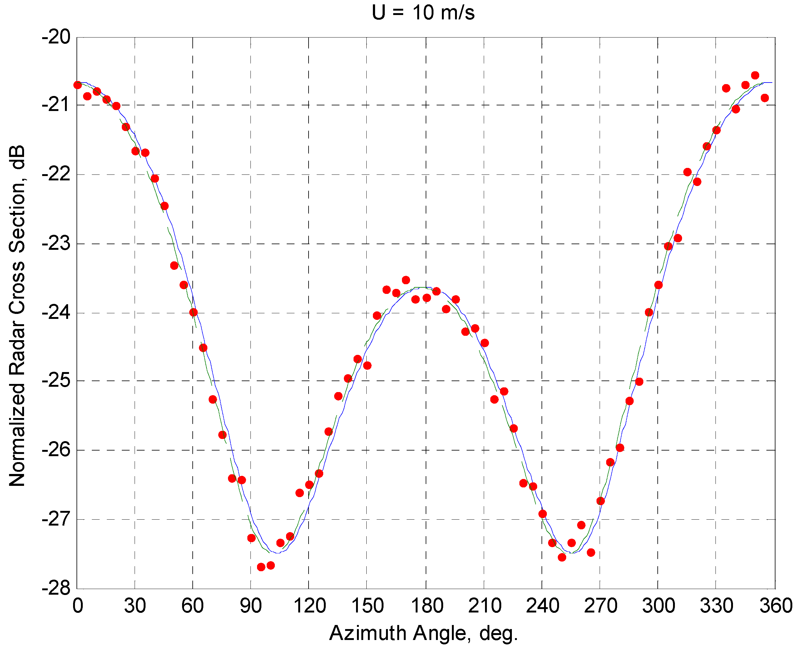
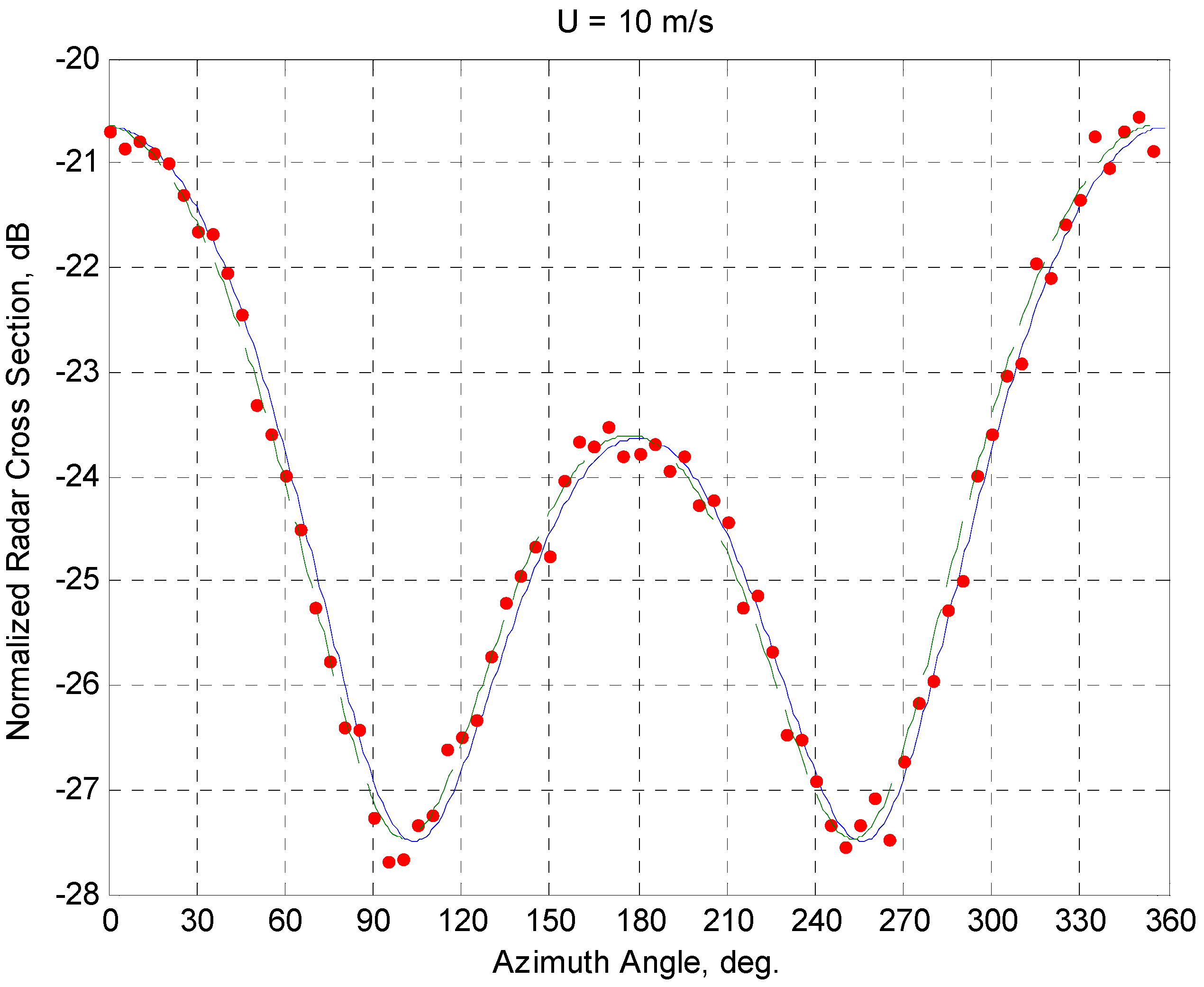
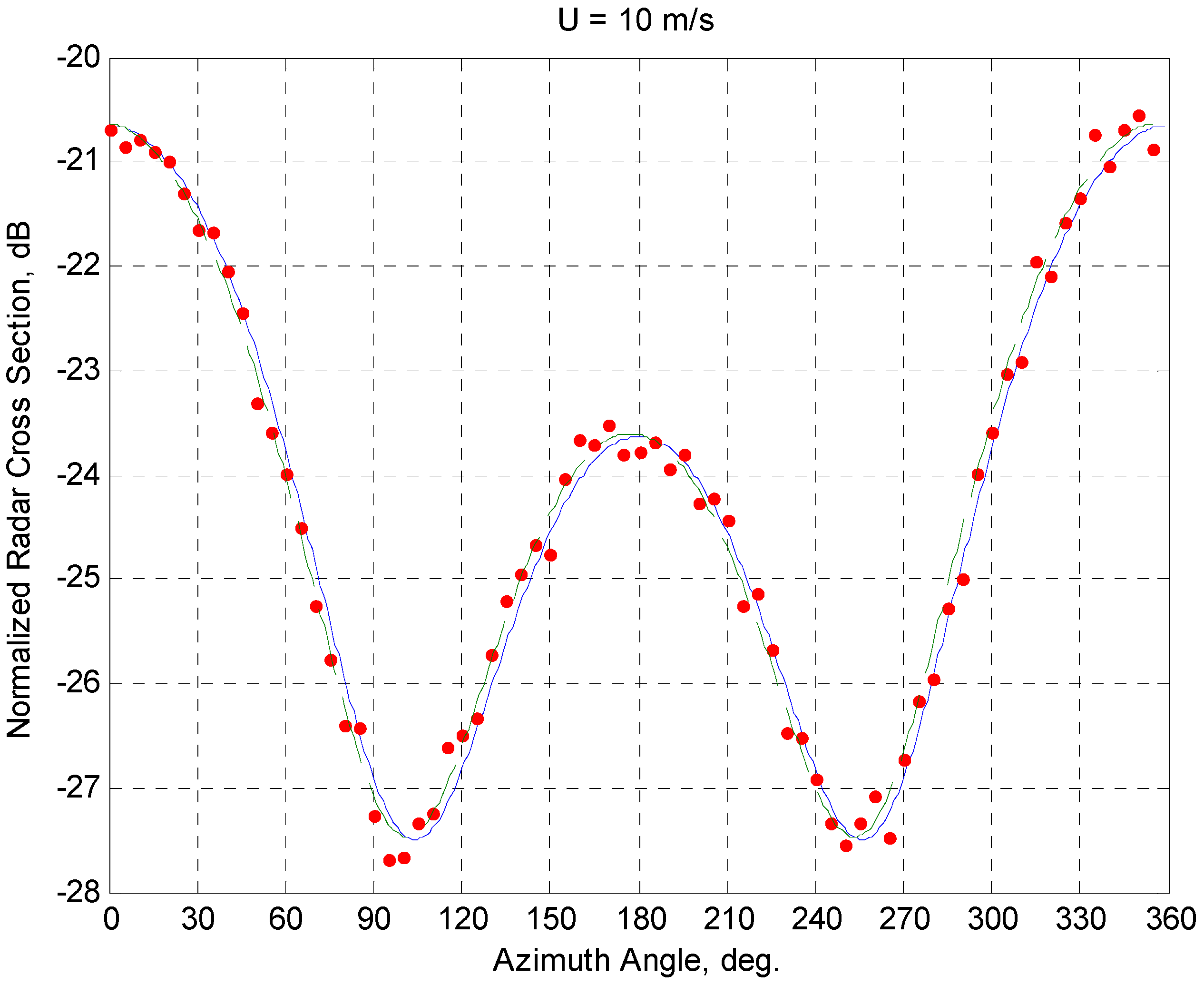
To investigate the performance and accuracy of the proposed wind algorithm, computer simulations of the wind vector retrieval procedure were performed. Since coefficients for the X-band geophysical model function of Equation (1) for the horizontal, transmitted and received, polarization could not be found in the current literature, our simulations used the function originally suggested for the neighboring Ku-band in [15]. This substitution is supported by the review of the NRCS values [5] indicating only modest differences between the X- and Ku-band backscatters. In our simulations, the incidence angle of 45° was considered. The “measured” azimuth NRCS values were generated using the Rayleigh Power (Exponential) distribution. A total of 1565 NRSC samples were integrated in each five-degree azimuth sector at the “true” wind speed of 10 m/s (Figure 2, Figure 3 and Figure 4, red dots) and then used in the system of Equation (4). Figure 2, Figure 3 and Figure 4 also present the azimuth NRCS curve using the model of Equation (1) at a given incidence angle, a “true” wind speed of 10 m/s and a “true” up-wind direction of 0° (solid lines) used for the generation of the “measured” NRCSs, and three examples of wind retrieval using NRCSs only from the following 180-degree azimuth sectors (dashed lines): [−90°, 90°], [45°, 225°], and [90°, 270°], respectively. The “measured” wind speeds and up-wind directions for these sector cases were 9.9718 m/s and 358.7°, 10.0071 m/s and 357.9°, 9.9975 m/s and 357.5°, respectively.
These results were obtained without considering instrumental noise. The instrumental measurement noise estimate for scatterometer measurements is about 0.2 dB, which corresponds to an uncertainty in wind speed of 0.5 m/s only [16]. Figure 5, Figure 6 and Figure 7 demonstrate simulation results for the wind estimation, taking into account the instrumental noise of 0.2 dB at the same conditions. The “measured” wind speeds and up-wind directions for the same sector cases were 9.994 m/s and 357.9°, 10.0258 m/s and 356.9°, 10.0279 m/s and 357.3°, respectively.
To summarize, our results clearly indicate the suitability and the accuracy of the proposed algorithm, even in the worst case of the 180-degree azimuth sector location of [90°, 270°].
In the case of the wind measurement over water, the range of incidence angles observed by the AWR in the ground-mapping mode should be extended from high to medium incidence angles for the better use of the anisotropic properties of water-surface scattering at medium incidence angles [4], as well as for power reasons [8]. For the water surface, the NRCS falls radically as the incidence angle increases, assuming different values for different conditions of sea state or water roughness, whereas, for most other types of terrain, the NRCS slowly decreases with an increase of the beam incidence angle [10]. Otherwise, the incidence angle of selected cell should be in the range of the validity of the NRCS model function of Equation (1) and should be out of the “shadow” region of water backscatter.
Considering that wind and wave conditions in different parts of the observational area are currently assumed to be identical, the measurement swath width, as well as the length of the area observed, should not exceed 15–20 km. Such a limitation of the observational area along with the AWR measurement geometry leads to the altitude limitations for the method’s applicability. The maximum altitude for a rectilinear flight will be about 10 km at the incidence angle of 45° and 5 km at the incidence angle of 60°, respectively.
The proposed concept and measurement principles considered in this paper could be used for the enhancement of the AWR, as well as for the development of an airborne radar system for operational measurement of the sea roughness characteristics and winds over water, which can not only be used for operational research but can also be applied to ensure the safe landing of seaplane or amphibious aircraft on water surfaces, especially during search-and-rescue missions or fire fighting in the coastal areas and fire risk regions complementing terrain avoidance systems [10,17].
Acknowledgments
We would like to acknowledge the financial support of this work by the Russian Science Foundation (project No. 16-19-00172). The authors would also like to express their sincere thanks to the Hamburg University of Technology for the research opportunities provided. A.N. would like to thank the German Academic Exchange Service (DAAD) for the support of an exchange visit.
Author Contributions
The authors contribute equally to this paper.
Conflicts of Interest
The authors declare no conflict of interest.
Abbreviations
The following abbreviations are used in this manuscript:
AWR
airborne weather radar
NRCS
normalized radar cross section
SAR
Synthetic Aperture Radar
References
Long, D.G.; Donelan, M.A.; Freilich, M.H.; Graber, H.C.; Masuko, H.; Pierson, W.J.; Plant, W.J.; Weissman, D.; Wentz, F. Current Progress in Ku-Band Model Functions; Technical Report MERS 96–002; Brigham Young University Press: Provo, UT, USA, 1996; p. 88. [Google Scholar]
Komen, G.J.; Cavaleri, L.; Donelan, M.; Hasselmann, K.; Hasselmann, S.; Janssen, P.A.E.M. Dynamics and Modelling of Ocean Waves; Cambridge University Press: Cambridge, UK, 1994; p. 532. [Google Scholar]
Ulaby, F.T.; Moore, R.K.; Fung, A.K. Microwave Remote Sensing: Active and Pasive, Volume II: Radar Remote Sensing and Surface Scattering and Emission Theory; Addison-Wesley: London, UK, 1982; p. 1064. [Google Scholar]
Masuko, H.; Okamoto, K.; Shimada, M.; Niwa, S. Measurement of microwave backscattering signatures of the ocean surface using X band and Ka band airborne scatterometers. J. Geophys. Res. Oceans1986, 91, 13065–13083. [Google Scholar] [CrossRef]
Li, L.; Heymsfield, G.; Carswell, J.; Schaubert, D.; McLinden, M.; Vega, M.; Perrine, M. Development of the NASA high-altitude imaging wind and rain airborne profiler. In Proceedings of the 2011 IEEE Aerospace Conference, Big Sky, MT, USA, 5–12 March 2011; pp. 1–8.
Sosnovsky, A.A.; Khaymovich, I.A.; Lutin, E.A.; Maximov, I.B. Aviation Radio Navigation: Handbook; Transport: Moscow, Russia, 1990; p. 264. (In Russian) [Google Scholar]
Yanovsky, F.J. Evolution and prospects of airborne weather radar functionality and technology. In Proceedings of ICECom 2005, Dubrovnik, Croatia, 11–14 October 2005; pp. 349–352.
Kayton, M.; Fried, W.R. Avionics Navigation Systems; John Wieley & Sons: New York, NY, USA, 1997; p. 773. [Google Scholar]
Nekrassov, A. On airborne measurement of the sea surface wind vector by a scatterometer (altimeter) with a nadir-looking wide-beam antenna. IEEE Trans. Geosci. Remote Sens.2002, 40, 2111–2116. [Google Scholar] [CrossRef]
Nekrasov, A. Water-surface wind vector estimation by an airborne weather radar having a medium-size scanning sector. In Proceedings of the 14th International Radar Symposium IRS 2013, Dresden, Germany, 19–21 June 2013; Volume 2, pp. 1079–1084.
Nekrasov, A. Airborne weather radar as a sensor of the wind vector over the water surface. In Proceedings of the Materialien zum wissenschaftlichen Seminar der Stipendiaten der Programme “Michail Lomonosov II” and “Immanuil Kant II” 2008/09, Moskau, Russia, 24–25 April 2009; pp. 155–158.
Nekrasov, A.; Popov, D. A concept for measuring the water-surface backscattering signature by airborne weather radar. In Proceedings of the 16th International Radar Symposium IRS 2015, Dresden, Germany, 24–26 June 2015; Volume 2, pp. 1112–1116.
Moore, R.K.; Fung, A.K. Radar determination of winds at sea. Proc. IEEE1979, 67, 1504–1521. [Google Scholar] [CrossRef]
Stoffelen, A. Scatterometry. Ph.D. Thesis, Utrecht University, Utrecht, The Netherlands, 1998; p. 209. [Google Scholar]
Labun, J.; Soták, M.; Kurdel, P. Technical note innovative technique of using the radar altimeter for prediction of terrain collision threats. J. Am. Helicopter Soc.2012, 57, 85–87. [Google Scholar] [CrossRef]
Figure 1.
Airborne weather radar (AWR) ground looking beam and selected cell geometry. V is the speed of flight; H is the aircraft altitude; θ is the incidence angle of the selected cell; ψ is the aircraft course; θa.v is the beamwidth in the vertical plane; θa.h is the beamwidth in the horizontal plane; Δαb is the angular resolution in the azimuthal plane; Δθ is the angular resolution in the vertical plane; is the current normalized radar cross section (NRCS) value.
Figure 2.
Azimuth NRCS curve using Equation (1) at the incidence angle of 45°, “true” wind speed of 10 m/s and “true” up-wind direction of 0° (solid line); generated “measured” NRCS after the averaging of 1565 samples in a five-degree azimuth sector (red dots); and azimuth NRCS curve using Equation (1) corresponding to “measured” wind speed of 9.9718 m/s and up-wind direction of 358.7° retrieved from the azimuth sector of [−90°, 90°] (dashed line).
Figure 3.
Azimuth NRCS curve using Equation (1) at the incidence angle of 45°, “true” wind speed of 10 m/s and “true” up-wind direction of 0° (solid line); generated “measured” NRCS after the averaging of 1565 samples in a five-degree azimuth sector (red dots); and azimuth NRCS curve using Equation (1) corresponding to “measured” wind speed of 10.0071 m/s and up-wind direction of 357.9° retrieved from the azimuth sector of [45°, 225°] (dashed line).
Figure 4.
Azimuth NRCS curve using Equation (1) at the incidence angle of 45°, “true” wind speed of 10 m/s and “true” up-wind direction of 0° (solid line); generated “measured” NRCS after the averaging of 1565 samples in a five-degree azimuth sector (red dots); and azimuth NRCS curve using Equation (1) corresponding to “measured” wind speed of 9.9975 m/s and up-wind direction of 357.5° retrieved from the azimuth sector of [90°, 270°] (dashed line).
Figure 5.
Azimuth NRCS curve using Equation (1) at the incidence angle of 45°, “true” wind speed of 10 m/s and “true” up-wind direction of 0° (solid line); generated “measured” NRCS with taking into account the instrumental noise of 0.2 dB after the averaging of 1565 samples in a five-degree azimuth sector (red dots); and azimuth NRCS curve using Equation (1) corresponding to “measured” wind speed of 9.994 m/s and up-wind direction of 357.9° retrieved from the azimuth sector of [−90°, 90°] (dashed line).
Figure 6.
Azimuth NRCS curve by model Equation (1) at the incidence angle of 45°, “true” wind speed of 10 m/s and “true” up-wind direction of 0° (solid line); generated “measured” NRCS with taking into account the instrumental noise of 0.2 dB after the averaging of 1565 samples in a five-degree azimuth sector (red dots); and azimuth NRCS curve by model Equation (1) corresponding to “measured” wind speed of 10.0258 m/s and up-wind direction of 356.9° retrieved from the azimuth sector of [45°, 225°] (dashed line).
Figure 7.
Azimuth NRCS curve using Equation (1) at the incidence angle of 45°, “true” wind speed of 10 m/s and “true” up-wind direction of 0° (solid line); generated “measured” NRCS with taking into account the instrumental noise of 0.2 dB after the averaging of 1565 samples in a five-degree azimuth sector (red dots); and azimuth NRCS curve using Equation (1) corresponding to “measured” wind speed of 10.0279 m/s and up-wind direction of 357.3° retrieved from the azimuth sector of [90°, 270°] (dashed line).
Nekrasov, A.; Khachaturian, A.; Veremyev, V.; Bogachev, M.
Sea Surface Wind Measurement by Airborne Weather Radar Scanning in a Wide-Size Sector. Atmosphere2016, 7, 72.
https://doi.org/10.3390/atmos7050072
AMA Style
Nekrasov A, Khachaturian A, Veremyev V, Bogachev M.
Sea Surface Wind Measurement by Airborne Weather Radar Scanning in a Wide-Size Sector. Atmosphere. 2016; 7(5):72.
https://doi.org/10.3390/atmos7050072
Chicago/Turabian Style
Nekrasov, Alexey, Alena Khachaturian, Vladimir Veremyev, and Mikhail Bogachev.
2016. "Sea Surface Wind Measurement by Airborne Weather Radar Scanning in a Wide-Size Sector" Atmosphere 7, no. 5: 72.
https://doi.org/10.3390/atmos7050072
APA Style
Nekrasov, A., Khachaturian, A., Veremyev, V., & Bogachev, M.
(2016). Sea Surface Wind Measurement by Airborne Weather Radar Scanning in a Wide-Size Sector. Atmosphere, 7(5), 72.
https://doi.org/10.3390/atmos7050072
Note that from the first issue of 2016, this journal uses article numbers instead of page numbers. See further details here.
Article Metrics
No
No
Article Access Statistics
For more information on the journal statistics, click here.
Multiple requests from the same IP address are counted as one view.
Nekrasov, A.; Khachaturian, A.; Veremyev, V.; Bogachev, M.
Sea Surface Wind Measurement by Airborne Weather Radar Scanning in a Wide-Size Sector. Atmosphere2016, 7, 72.
https://doi.org/10.3390/atmos7050072
AMA Style
Nekrasov A, Khachaturian A, Veremyev V, Bogachev M.
Sea Surface Wind Measurement by Airborne Weather Radar Scanning in a Wide-Size Sector. Atmosphere. 2016; 7(5):72.
https://doi.org/10.3390/atmos7050072
Chicago/Turabian Style
Nekrasov, Alexey, Alena Khachaturian, Vladimir Veremyev, and Mikhail Bogachev.
2016. "Sea Surface Wind Measurement by Airborne Weather Radar Scanning in a Wide-Size Sector" Atmosphere 7, no. 5: 72.
https://doi.org/10.3390/atmos7050072
APA Style
Nekrasov, A., Khachaturian, A., Veremyev, V., & Bogachev, M.
(2016). Sea Surface Wind Measurement by Airborne Weather Radar Scanning in a Wide-Size Sector. Atmosphere, 7(5), 72.
https://doi.org/10.3390/atmos7050072
Note that from the first issue of 2016, this journal uses article numbers instead of page numbers. See further details here.


