Article

Composition and Sources of Particulate Matter Measured near Houston, TX: Anthropogenic-Biogenic Interactions

by
Jeffrey K. Bean
1,
Cameron B. Faxon
1,
Yu Jun Leong
2,
Henry William Wallace
2,
Basak Karakurt Cevik
2,
Stephanie Ortiz
3,
Manjula R. Canagaratna
4,
Sascha Usenko
3,
Rebecca J. Sheesley
3,
Robert J. Griffin
2 and
Lea Hildebrandt Ruiz
1,*
1
McKetta Department of Chemical Engineering, The University of Texas at Austin, Austin, TX 78712, USA
2
Department of Civil and Environmental Engineering, Rice University, Houston, TX 77005, USA
3
Department of Environmental Science, Baylor University, Waco, TX 76798, USA
4
Aerodyne Research Inc., Billerica, MA 01821, USA
*
Author to whom correspondence should be addressed.
Atmosphere 2016, 7(5), 73; https://doi.org/10.3390/atmos7050073
Submission received: 6 April 2016 / Revised: 6 May 2016 / Accepted: 17 May 2016 / Published: 23 May 2016
(This article belongs to the Special Issue Air Quality and Source Apportionment)

Abstract

:
Particulate matter was measured in Conroe, Texas (~60 km north of downtown Houston, Texas) during the September 2013 DISCOVER-AQ campaign to determine the sources of particulate matter in the region. The measurement site is influenced by high biogenic emission rates as well as transport of anthropogenic pollutants from the Houston metropolitan area and is therefore an ideal location to study anthropogenic-biogenic interactions. Data from an Aerosol Chemical Speciation Monitor (ACSM) suggest that on average 64 percent of non-refractory PM1 was organic material, including a high fraction (27%–41%) of organic nitrates. There was little diurnal variation in the concentrations of ammonium sulfate; however, concentrations of organic and organic nitrate aerosol were consistently higher at night than during the day. Potential explanations for the higher organic aerosol loadings at night include changing boundary layer height, increased partitioning to the particle phase at lower temperatures, and differences between daytime and nighttime chemical processes such as nitrate radical chemistry. Positive matrix factorization was applied to the organic aerosol mass spectra measured by the ACSM and three factors were resolved—two factors representing oxygenated organic aerosol and one factor representing hydrocarbon-like organic aerosol. The factors suggest that the measured aerosol was well mixed and highly processed, consistent with the distance from the site to major aerosol sources, as well as the high photochemical activity.

Graphical Abstract

1. Introduction

Air quality in the United States has received increased attention in recent years as regulations tighten and cities strive to reduce concentrations of airborne pollutants. Ozone and atmospheric particulate matter (PM) are two pollutants that have received increased attention as health effects become clearer [1]. Particulate matter is linked to a range of respiratory and cardiovascular diseases [2]. High ozone levels can also lead to respiratory problems [3]—especially in more sensitive groups such as children, the elderly, and those with asthma. Many regions struggle to meet compliance with the National Ambient Air Quality Standard (NAAQS) [4] for ozone and PM set by the U.S. Environmental Protection Agency (EPA).
The U.S. EPA recently lowered the annual NAAQS for PM2.5 (particulate matter with diameter below 2.5 μm) from 15 to 12 µg·m−3 [5]. This new annual standard brings numerous additional metropolitan regions including Houston, TX to near non-attainment for PM2.5. This underlines the importance of understanding the composition and sources of PM2.5 in these areas. The EPA has also announced that the NAAQS for ozone will be lowered from 75 to 70 ppb [6]—a level that will require action for many metropolitan regions. Houston is an important area for air quality research as the fourth largest U.S. city and one that struggles to meet air quality standards. As a major center for the energy and chemical industry, Houston must continuously inspect, analyze, and improve its air quality in order to stay below the NAAQS and improve the health of its inhabitants. Regional photo-chemical models are used to inform policy makers, but these models must be validated with ambient measurements. Measurements can also be used for source apportionment of air pollution.
Recognizing the importance of ambient measurements, several large-scale ambient measurement campaigns have been conducted in Texas [7]. The biggest campaign was the Texas Air Quality Study in 2000 (TexAQS 2000). A key discovery of this campaign was the important role of highly reactive volatile organic compounds (HRVOCs) in ozone production [8]. The Gulf Coast Aerosol Research and Characterization Study (GC-ARCH), a companion study to TexAQS, was focused on spatial and temporal variability in PM, as well as understanding its formation and transformation in southeast Texas [9]. The TexAQS 2000 campaign was followed up with TexAQS II in 2005–2006, a key finding of which was the magnitude of background concentrations of pollutants in Texas, which adds to the complexity of understanding and improving air quality. The 2009 Study of Houston Atmospheric Radical Precursors (SHARP) campaign uncovered the previously underestimated role of nitrous acid (HONO) in Texas air [10]. Since 2010, many smaller-scale studies in Texas have added to our understanding of the complex effects of oil and gas activity on air quality [11,12,13]. The amount of effort that has been applied towards understanding air quality in Texas highlights the importance of this research in meeting NAAQS and improving human health.
Previous studies have found that a large fraction of particulate matter in Houston is organic aerosol (OA) [9,14]. Sources of OA in Houston include primary organic aerosol (POA) and secondary organic aerosol (SOA) [15] from urban anthropogenic activity, the petrochemical industry, and fires, as well as SOA from biogenic volatile organic compounds (VOCs) [9,14,16]. Understanding the sources and formation of OA is therefore very complex, and significant uncertainties remain. Conroe, TX, the location of the measurements reported here, is located ~60 km north of the urban center of Houston. The measurement site is in an area that is influenced by anthropogenic emissions from Houston that have been diluted and atmospherically processed since emission. The area is subject to high biogenic emission rates and is located near the start of the piney woods that extend through the US Southeast—a big difference from the grassy prairies that extend west and south throughout Texas. This ecosystem transition near Conroe makes it an interesting place to explore the effects of the ecosystems on observed PM. The interaction of biogenic VOCs and anthropogenic oxidants is very important as it helps explain why radiocarbon analysis in places like the U.S. Southeast show that biogenic (modern) carbon constitutes more than half of SOA, yet SOA correlates with anthropogenic tracers like CO [17]. Recent work [18,19,20] has begun to explore these interactions and their implications for air quality in places with high levels of biogenic VOCs.
Here we report measurements taken as part of Deriving Information on Surface Conditions from Column and Vertically Resolved Observations Relevant to Air Quality (DISCOVER-AQ) [21] during the period of 24 August–1 October 2013. A main purpose of this most recent large-scale ambient measurement campaign, which was organized through NASA, was to improve the interpretation of ground-level pollutant concentrations from satellite data by taking simultaneous measurements from space, by plane and on the ground. This manuscript focuses on measurements taken at a ground site in Conroe, TX, where various instruments were deployed. The focus of this work is the composition and size distribution of PM1 (particulate matter with diameter below 1 µm), which was measured with an Aerosol Chemical Speciation Monitor (ACSM) and a Scanning Electrical Mobility Spectrometer (SEMS). The purpose of these measurements was to better characterize the sources and processes which influence the concentrations of PM in this area. An improved understanding of Houston PM is essential in formulating ways to decrease concentrations and more generally manage the air quality in this region.

2. Experimental

2.1. Site Description

The data were obtained at an air quality monitoring ground site in Conroe, TX (30.350278° N, 95.425000° W) situated next to the Lone Star Executive Airport in Montgomery county. The site is located approximately 60 km NNW from the Houston, TX urban center and approximately 125 km NW of the nearest coastline. The area surrounding Conroe, TX is primarily affected by pollution in the outflow of air from Houston, which hosts significant energy and petrochemical industries in addition to a large urban population. The regional atmospheric chemistry is also influenced by marine air from the Gulf of Mexico. The site itself is located in the middle of a field adjacent to the airport, with a gravel parking lot nearby and bordered by trees approximately 200 m to the North. The Conroe region is where the ecosystem transforms from prairie and marsh to piney woods, which then extend north and east through much of the Southeastern United States.

2.2. Instrumentation and Data Analysis

A permanent Texas Commission on Environmental Quality (TCEQ) ambient measurement station exists at this site and provided continuous meteorological data for the duration of the campaign [22]. Measured parameters included wind speed, wind direction, solar irradiance, temperature, and relative humidity. The site also housed NOx and O3 monitors, as well as a Tapered Element Oscillating Microbalance (TEOM) for measurements of PM2.5 mass concentrations. During DISCOVER-AQ a temporary ground site (an air-conditioned trailer) was set up adjacent to the permanent station. This temporary site housed an NO2 monitor (Model AS32M from Environnement) which utilizes cavity attenuated phase shift spectroscopy (CAPS) to provide a direct absorption measurement of nitrogen dioxide [23]. NOx was measured using a chemiluminescence NOx monitor (Teledyne Model 200E), and O3 was measured by direct UV absorption (Teledyne, 400E). An Aerosol Chemical Speciation Monitor (ACSM, Aerodyne Research) [24] was used to measure the mass concentrations of non-refractory species in PM1 including sulfate, nitrate, ammonium, and organics. A Scanning Electrical Mobility System (SEMS, Brechtel Manufacturing) was used to characterize particle size distributions and mass concentrations of PM1. A High Resolution Time-of-Flight Chemical Ionization Mass Spectrometer (HR-ToF-CIMS, Aerodyne Research) [25,26,27,28] was employed to measure gas-phase species. All sample lines extended out the trailer and to a vertical level of approximately 10 feet. Teflon® tubing (1/4 inch) was used to sample all gas-phase compounds and copper tubing (1/2 inch) was used for particle-phase instruments.
Filter measurements of PM2.5 were taken on site as described in Section 2.2.4. During approximately 61 h of the campaign the University of Houston-Rice University mobile air quality laboratory (MAQL) was parked at the measurement site. The instrumentation on the MAQL included a suite of photochemical trace gas instrumentation, a photoacoustic spectrometer for measurement of particle-phase polycyclic aromatic hydrocarbons, and a High-Resolution Time-of-Flight Aerosol Mass Spectrometer (HR-ToF-AMS, Aerodyne Research). The HR-ToF-AMS measures the same PM1 species as the ACSM but in a size-resolved manner based on the vacuum aerodynamic diameter, and the time of flight mass spectrometer enables measurements at much higher mass and time resolution. The co-location of the HR-ToF-AMS and the ACSM enables comparison of PM1 measurements.

2.2.1. Aerosol Chemical Speciation Monitor

Data analysis and instrument operation were performed in IGOR Pro (WaveMetrics) using the “ACSM Local” software package. The ACSM was set to scan between m/z 12 and 159 with a dwell time of 0.5 s, resulting in a scan time of 80 s. The instrument was set to alternate between sampling mode and filter mode, where the filter sample is used to characterize the gas-phase background. This results in a cycle time of 160 s. Further averaging over 25 min intervals was performed in the post-analysis of the data (see Appendix A). The vaporizer temperature was set at 600 °C (as is standard) for fast vaporization of ammonium sulfate. The ACSM measures only non-refractory (NR) PM1, i.e. compounds that flash vaporize at the heater temperature of 600 °C. Quantification of aerosol concentrations measured by the ACSM is complicated by incomplete transmission of larger particles through the aerodynamic lens and particle bounce at the vaporizer. The ACSM collection efficiency (CE) for these data was estimated to be 0.5, which resulted in good agreement with ancillary measurements (Figure A1). Additional details on instrument calibration, data preparation, and adjustments to the standard fragmentation table [29] are provided in Appendix A. The HR-ToF-AMS operates similarly to the ACSM but at higher mass and time resolution due to its time of flight mass spectrometer (as opposed to the quadrupole mass spectrometer used by the ACSM). Details on the HR-ToF-AMS operation and data collected during the DISCOVER-AQ campaign will be presented in a forth coming publication [30].
The ACSM provides two main measures of PM1: bulk composition (concentrations of organics, nitrate, sulfate, and ammonium) and the total mass spectrum from which the organic mass spectrum can be derived. The organic mass spectrum can be used to characterize the extent of oxidation of the measured organic aerosol. The organic mass at m/z 44 mostly correspond to the CO2+ ion [31] and can therefore be used as a semi-empirical measure of the extent of oxidation in the system. Aiken et al. [31] showed that f44, the fraction of the total organic signal due to mass at m/z 44, can be used to estimate the oxygen to carbon ratio (O:C) in the organic aerosol. The correlation between O:C and f44 was recently updated to [32]:
(O:C)f44 = 4.31 × f44 + 0.079
Aiken et al. [31] also found a significant correlation between the ratio of organic mass to organic carbon (OM:OC) and O:C. This relationship was found to be applicable to field data as well as laboratory data and is described by:
(OM:OC) = 1.29 × O:C + 1.17
Thus, the observed f44 can be used to estimate O:C and OM:OC of the organic aerosol measured at Conroe. These estimates can be compared with values from the HR-ToF-AMS, which directly computes O:C and OM:OC from elemental analysis of the high resolution measurements (see Appendix B).

2.2.2. Positive Matrix Factorization

Positive Matrix Factorization (PMF) was applied to the organic aerosol mass spectra measured by the ACSM [33]. The PMF2 algorithm (version 4.2) by P. Paatero was used to solve the bilinear unmixing problem as represented and described below. PMF has proven useful in the analysis of ambient organic aerosol data, and details of the mathematical model, its application, output evaluation, and factor interpretation have been described elsewhere [34,35,36,37,38]. A key assumption is that the measured dataset can be separated into a number of constant components (here, ACSM mass spectra) contributing varying concentrations over time. The problem is represented in matrix form by:
X = G F + E
where X is an m × n matrix of the measured data with m rows of average mass spectra (number of time periods = m) and n columns of time series of each m/z sampled (number of m/z sampled and fit = n). F is a p × n matrix with p factor profiles (constant mass spectra), G is an m × p matrix with the corresponding factor contributions, and E is the m × n matrix of residuals. G and F are fit to minimize the sum of the squared and uncertainty-scaled residuals [33]. The number of factors is chosen by determining when added factors fail in explaining additional dataset variability.
The ACSM dataset was prepared for PMF analysis by first selecting only organic fragments below m/z 100, as higher m/z fragments exhibited very low concentrations and added significant error to the analysis. Peaks with a signal to noise ratio below 2 were downweighted by a factor of 2. The peaks, which are calculated from m/z 44 (m/z 16–18.44), were downweighted to remove the extra influence of m/z 44 on PMF solutions. The PMF2 algorithm was used in exploration mode with fpeak set from −1 to 1 by 0.2 increments.

2.2.3. High Resolution Time of Flight Chemical Ionization Mass Spectrometer

The HR-ToF-CIMS was set to alternate between positive (hydronium-water clusters) and negative (iodide-water clusters) chemical ionization in half hour intervals. Hydronium-water cluster ionization is more sensitive than iodide-water cluster ionization to less oxidized compounds such as early oxidation products from terpenes and isoprene. For both cases ultra-high purity N2 was first passed through water, then across a methyl iodide permeation tube, and then ionized as it passed through a radioactive source of Po-210. The increased humidity helped dampen the effects of the changing RH in the sample gas. Ionized compounds were pulsed in a “V” shape through a time-of-flight region during measurement to obtain a mass spectrum. Some data obtained through iodide ionization have been described previously [39] and here we focus on data from water cluster ionization.
Data from the HR-ToF-CIMS were analyzed in Igor Pro (Wavemetrics) using Tofware, the software provided with the instrument. The data were first mass calibrated based on HR-ToF-CIMS reagent ions and other known ions. The baseline was subtracted and the average peak shape was found so it could be used for high resolution analysis, through which multiple ions can be identified at any given integer mass to charge ratio (m/z). Analyte ion concentrations were then normalized by dividing by the reagent ion concentrations, the sum of H3O+, H3O+(H2O) and H3O+(H2O)2,and then multiplying by the average sum of the three reagent signals (to maintain the units of ion counts s−1).

2.2.4. Filter Measurements

A high volume PM2.5 sampler (Tisch Environmental, Cleves, OH, USA; 226 lpm), on loan from the US EPA, was used to collect daily samples. PM2.5 samples were collected over 23.5 h (6 a.m. to 5:30 a.m.). Sample media consisted of quartz fiber filters (QFF) which were baked at 550 °C for 12 h in individual foil packets prior to sampling. QFF were stored in freezers (−10 °C) pre- and post-sampling. PM2.5 was collected on 102 mm diameter QFF (Pall Corporation, Port Washington, NY, USA), and samplers were calibrated prior to field deployment. Field blanks were collected throughout the campaign for each type of sampler and handled in the same manner as ambient samples. The QFF were analyzed for organic and elemental carbon (OCEC) using a thermal-optical method (NIOSH-5040) on Baylor University’s thermo-optical transmission (TOT) carbon analyzer (Sunset Laboratories, Tigard, OR, USA) [40]. Sample aliquots were also sent to the Desert Research Institute (DRI-Nevada) for inorganic ion analysis (sulfate, nitrate, ammonium, chloride and potassium).
Radiocarbon abundance (14C) was analyzed on filter samples in order to determine the contributions of contemporary and fossil emissions to Houston’s ground-based carbonaceous PM. Contemporary sources include biomass burning and biogenic emissions, and they include the presence of 14C. Fossil sources include combustion and non-combustion emission sources with depleted 14C. Ambient PM2.5 filter subsamples were taken for analysis to give ~60 µg of total organic carbon [41] for measurement of the 14C signal on the accelerator mass spectrometer. Subsamples were acidified over hydrochloric acid using a desiccator for 12 h to remove carbonate, and dried in a muffler oven at 60 °C for one hour. 14C abundance measurements were performed at the National Oceanic Sciences Accelerator Mass Spectrometry (NOSAMS) facility at Woods Hole Oceanographic Institute (Woods Hole, MA, USA).
In order to apportion total organic carbon (TOC) based on 14C abundance, Δ14C end members are chosen based on the sampling region and used in the following equation:
Δ 14 C s a m p l e = Δ 14 C c o n t e m p o r a r y × f c o n t e m p o r a r y +   Δ 14 C f o s s i l × ( 1 f c o n t e m p o r a r y )  
The contemporary end member used for this study was 67.5‰, an average of the 2010 biomass burning end member (Δ14C = 107.5‰) corresponding to wood smoke and the 2010 biogenic end member (Δ14C = 28‰) corresponding to primary and secondary biogenic emissions, meat cooking and combustion of grass, prunings and agricultural waste [42,43]. The fossil fuel end member was −1000‰ [44]. Results from NOSAMS are reported as % contemporary, with contribution from fossil carbon equaling 1-fcontemporary.

2.2.5. Diurnal Patterns: Analysis of Statistical Significance and Patterns

We conducted one-way analysis of variance (ANOVA) tests for organics, sulfate, nitrate and each PMF factor as dependent variables with time of day as the independent variable. ANOVA tests determine whether there are statistically significant differences in the mean values of the dependent variables [45]. While ANOVA tests determine statistical significance of variation by time of day, they cannot quantify or characterize the diurnal cycle. Thus, we also conducted harmonic analysis [45,46] to characterize the diurnal cycle. In brief, the general harmonic function is given by:
y t = y ¯ + C k c o s ( 2 π t / n k )
where t is the time (1–24 in our diurnal analysis), y ¯ is the mean of the time series (e.g., yt is the mean value of f44 during hour t, y ¯ is the mean value for the whole campaign), Ck is the amplitude of the kth harmonic, n is the period (n = 24 here) and ϕ is the phase. Using only the first harmonic, we can estimate the amplitude by [45,46]:
C 1 = [ A 1 2 + B 1 2 ] 1 / 2
where
A 1 = 2 / n × y t c o s ( 2 π t / n )
B 1 = 2 / n × y t s i n ( 2 π t / n )
The phase is then given by:
φ 1 = t a n 1 ( B 1 / A 1 ) ± π   if  A 1 < 0
φ 1 = t a n 1 ( B 1 / A 1 )   if  A 1 > 0
φ 1 = π / 2   if  A 1 = 0
The portion of the variance explained by the first harmonic, analogous to a correlation coefficient (R2) commonly computed in regression analysis, is given by:
V 1 = C 1 2 / 2 s 2
where s is the standard deviation of the n values. The phase simply describes to what extent the observed cycle is offset from a standard cosine curve. The amplitude describes the magnitude of the diurnal cycle.

3. Results

This work combines PM measurements from several different instruments. Measurements from different instruments generally agreed well as discussed in Appendix B.

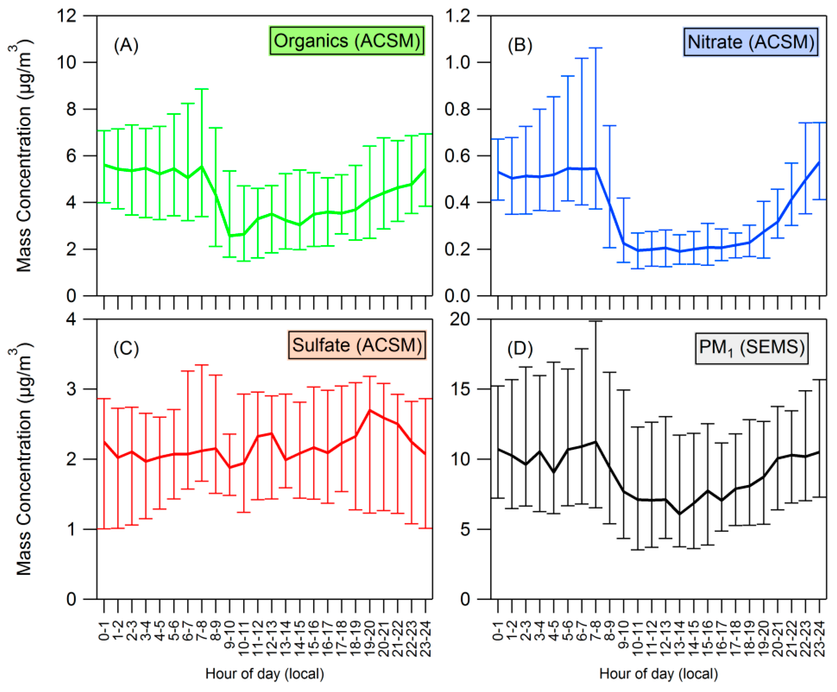
3.1. Bulk Concentrations and Diurnal Cycle

Figure 1 shows a time series of particle size distributions (top), a time series of bulk concentrations measured by the ACSM (bottom), and the campaign-average bulk concentration (right). The ACSM nitrate measurements (sum of NO+ and NO2+ fragments) can be attributed to inorganic nitrate and/or -ONO2 functional groups on organic nitrates. Measurements indicate that the nitrate measured by the ACSM in Conroe is mostly organic. One indication of this is the NO+:NO2+ ratio in ACSM measurements, which is estimated from the fragmentation table-corrected unit mass resolution data. In the ACSM used for this study a ratio of 2.6–3.9 has been measured for ammonium nitrate. For organic nitrate this ratio has varied but has always been greater than 5 for this instrument. The average NO+:NO2+ ratio for this data set is 13.4, which is consistent with organic nitrate (and inconsistent with ammonium nitrate). Filter measurements also indicate that nitrate measured by the ACSM was mostly organic (see Appendix B): filter measurements of inorganic nitrate are significantly lower than ACSM measurements of total nitrate (Figure A4C). Further, the molar ratio of NH4:SO4 indicates that on average there was no excess NH4 as required for the formation of ammonium nitrate.
As seen in Figure 1, a large portion of PM1 measured in Conroe was organic (64% on average, including nitrate). PM composition from filter measurements agreed with ACSM measurements—71% of PM from the filter samples was OM, with most of the remainder being ammonium and sulfate (as well as 1.7% EC). Sulfate is a significant part of PM1 in Conroe. Ammonium concentrations were often below the detection limit of the ACSM but when it was measured, the aerosol had an average ammonium/sulfate molar ratio of 2. Figure 1 also shows the PM1 number distributions from the SEMS. Nucleation events are not easily identified and do not seem to play a major role in PM concentrations in this area during this time period.
Consistent diurnal profiles were seen for both organics and nitrate in PM1 measurements. Figure 2 shows the average (median) diurnal variation of organics, nitrate, sulfate and total PM1 measured by the SEMS; the error bars indicate the 25th and 75th percentiles. ANOVA reveals statistically significant variation by time of day for organic, nitrate, and total PM1 concentrations (p < 10−16), but no statistically significant variation by time of day for sulfate concentrations (p = 0.65). Harmonic analysis suggests that the phase (between 0 and 2π) for these diurnal trends is 0.4, 0.7, and 0.5 for organics, nitrate, and (SEMS) PM1 respectively-indicating that concentrations of these species increase and decrease at approximately the same time. The first harmonic explains 78%, 88% and 87% of the variance for organics, nitrate, and (SEMS) PM1, respectively. The analysis further reveals that the amplitude-to-mean ratio of the nitrate diurnal is 0.55, compared to the amplitude-to-mean ratio of the organics and PM1 diurnal profiles which are 0.29 and 0.20, respectively.

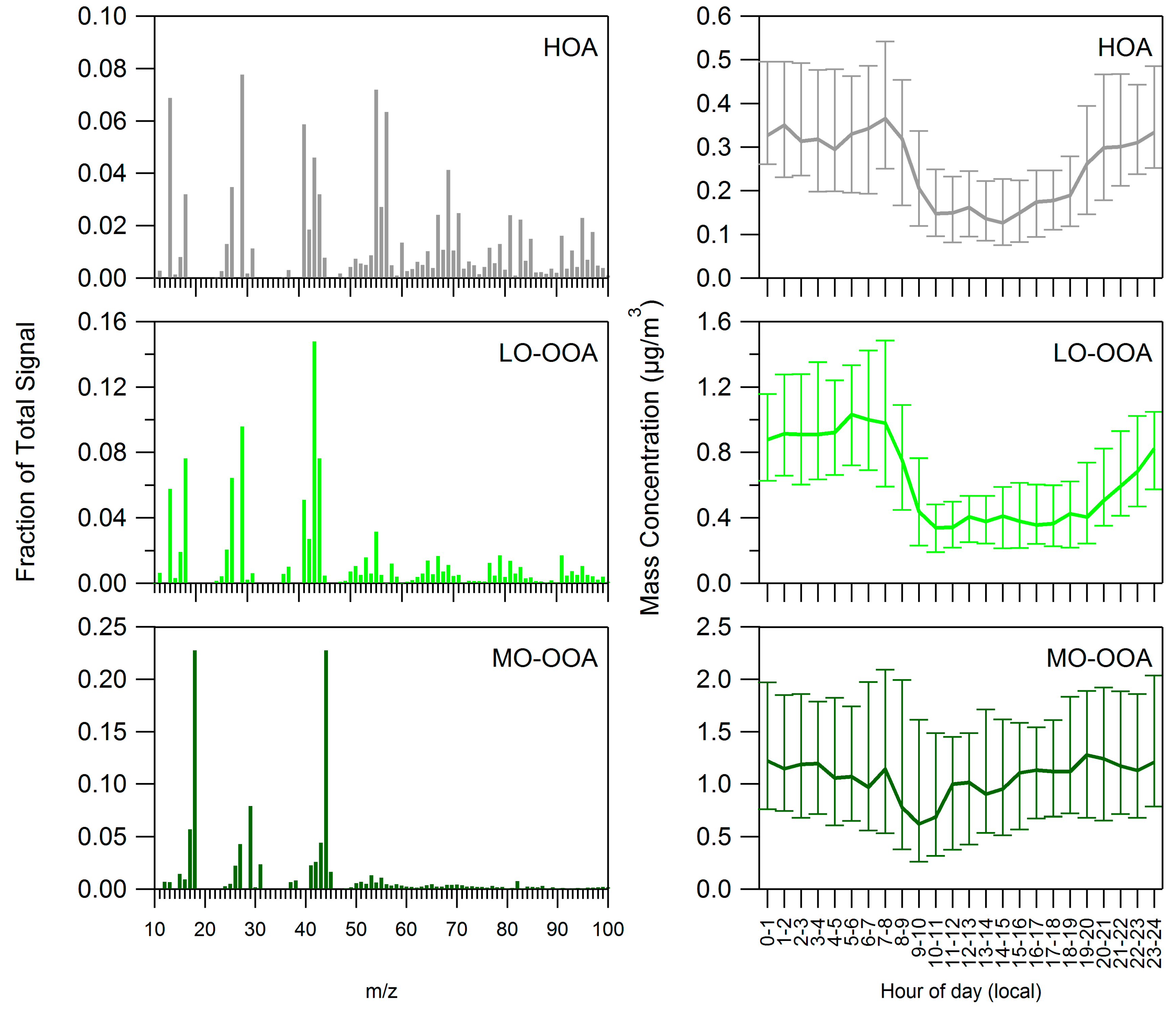
3.2. Positive Matrix Factorization

Various PMF solutions (obtained by varying the number of factors and other PMF settings, See Section 2.2.2) were examined and evaluated with respect to mathematical diagnostics and ancillary data (not included in the PMF analysis, e.g., ACSM-sulfate). The three-factor solution was found to best represent these data. Possible solutions of up to 8 factors were considered but factor splitting was observed and no additional information was obtained from the use of more than three factors.
The mass spectra and diurnal cycles of the three factors are shown in Figure 3. Two of the factors resemble oxygenated organic aerosol (OOA), the other factor resembles fresher organic aerosol. We name the more oxidized OAA factor (f43 = 4.4%, f44 = 22.7%) MO-OOA (more oxidized OOA) and the less oxidized OOA factor (f43 = 14.8%, f44 = 7.6%) LO-OOA (less oxidized OOA). The third factor has mass spectral signatures representative of hydrocarbon like organic aerosol (HOA) and biomass burning organic aerosol (BBOA), but we refer to the third factor (f43 = 4.6%, f44 = 3.2%) as HOA for simplicity.
The time series of MO-OOA showed a correlation with the time series of sulfate measured by the ACSM (R2 = 0.46), whereas LO-OOA did not (R2 = 0.10). Thus, MO-OOA correlated with a low-volatility inorganic component (sulfate). LO-OOA and HOA showed correlation with NOx (R2 = 0.35 and 0.34, respectively), a proxy for fresh anthropogenic emissions, while MO-OOA did not (R2 = 0.06). We also examined correlations of the factor profiles with factor profiles identified in previous work [47]. The MO-OOA profile correlated most strongly with previously identified MO-OOA (R2 = 0.92), the LO-OOA profile correlated most strongly with previously identified LO-OOA (R2 = 0.92), and the HOA correlated most strongly to previously identified HOA (R2 = 0.67) and BBOA (R2 = 0.74).
Figure 3 (right panel) shows the diurnal cycle of the three PMF factors. According to ANOVA, all three factors exhibited statistically significant variation by time of day (p < 10−16 for HOA and LO-OOA, p = 6 × 10⁻⁸ for MO-OOA). LO-OOA and HOA exhibited a clear pattern with higher concentrations at night, the same pattern exhibited by total OA (see Section 3.1). MO-OOA did not show this clear pattern, presumably because during the afternoon some LO-OOA and HOA is converted to the MO-OOA, which is more highly oxidized. MO-OOA can also form directly from oxidized VOCs. Harmonic analysis suggests that the diurnal cycle of LO-OOA has an amplitude-to-mean ratio of 0.53 and phase of 0.8 and can explain 84% of the variance; the diurnal cycle of HOA has an amplitude-to-mean ratio of 0.41, phase of 0.5 and can explain 79% of the variance. These two PMF factors (LO-OOA and HOA) hence have diurnal cycles of similar phase, which is also similar to the phase of the diurnal cycle of total OA (Section 3.1).
Figure 4 shows time series of the factors in terms of fraction of total organics (the sum of all 3 factors). The 12 days before 6 September were included in PMF calculations but excluded from Figure 4 to facilitate viewing of radiocarbon results. HOA can constitute 30% or more of OA on days when overall PM concentrations are low (7 September, 16–21 September). However, fresh emissions represented by HOA constitute a smaller fraction (less than 20%) of PM on high concentrations days, such as 10–15 September and 25–28 September. On these higher concentration days a larger fraction of the increased PM levels are due to MO-OOA (and LO-OOA to a lesser extent), consistent with atmospheric conditions which transport highly processed OA or allow existing OA to become highly oxidized. The results of radiocarbon analysis (see Section 2.2.4) are also shown in Figure 4. Fossil carbon constituted as little as 10% of carbon in OA during the low concentration period from 21–23 September but was approximately 30% of carbon during the high concentration period from 25–28 September, suggesting that a higher fraction of OA originates from fossil sources of carbon on higher concentrations days.

4. Discussion

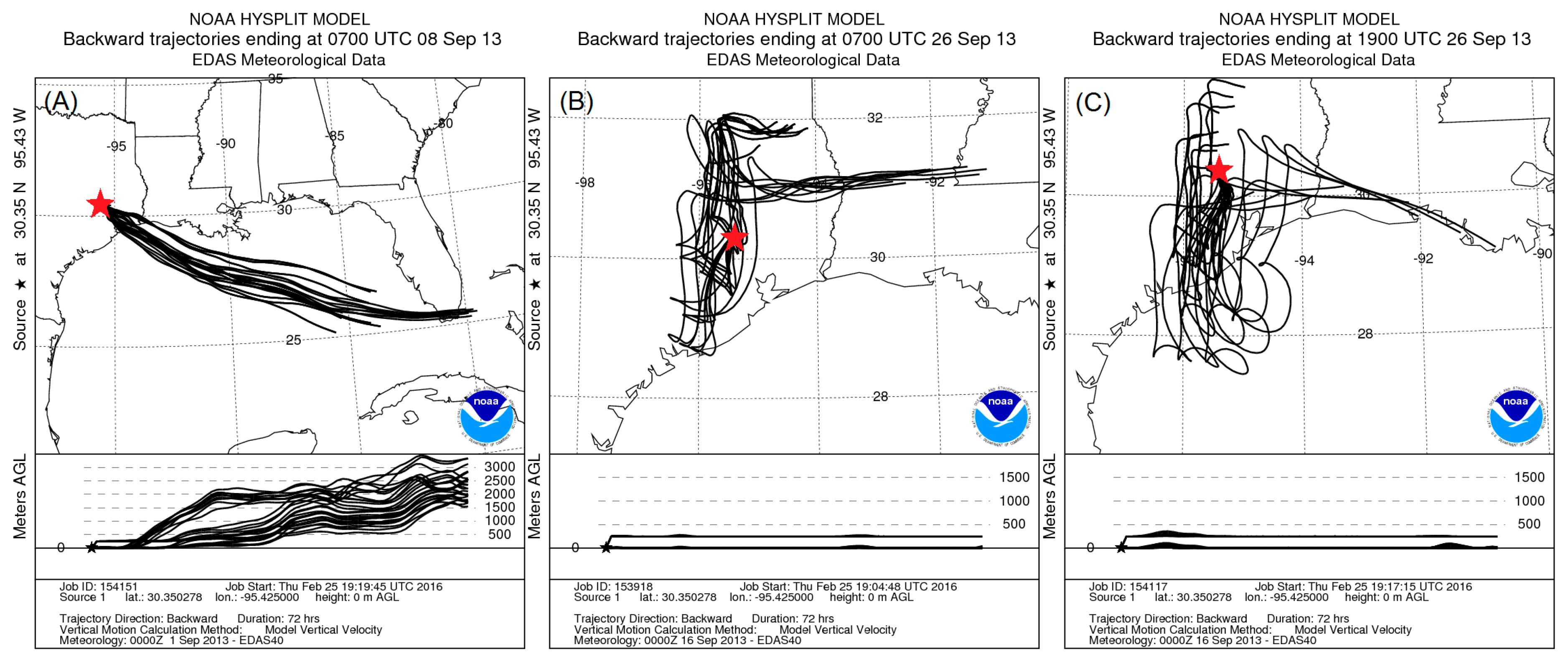
4.1. Composition of PM and Source Regions

Because very little inorganic nitrate appears to be present (see Section 3.1), we assume that all nitrate measured by the ACSM is organic in order to estimate the organic nitrate contribution to organic aerosol. For an assumed MW range of 200–300 g·mol−1 [48] organic nitrates constitute 27%–41% of organic aerosol. If nitrate was overestimated by up to 60% (Figure A3) then organic nitrates would still constitute 18%–27% of OA. Either estimate would suggest that organic nitrates play a larger role in Conroe than has been measured in other areas. Using the same estimate for molecular weight of organic nitrates, Xu et al. [19] estimated that organic nitrates constitute 5%–16% of OA during the summer in Alabama and Georgia locations. Mylones et al. [49] assumed an average molecular weight of 150 g·mol−1 for organic nitrates and calculated that they are 13% of OA in Los Angeles. Studies in Houston using the same methods as Mylones et al. have observed an organic nitrate fraction similar to the one observed in Los Angeles [50,51]. O’Brien et al. [52] estimated organic nitrates constituted 17% of OA in Los Angeles in 1975. The prominence of organic nitrates in OA highlights the importance of anthropogenic emissions for this region as nitrate formation requires anthropogenic NOx or NO3 in addition to VOCs.
Concentrations of PM1 vary both diurnally and over the course of several days. Increases and decreases in PM1 concentrations in the timeframe of days and weeks are often associated with changes in regional air flow. Figure 5 shows 72-h back trajectories calculated using the Hybrid Single Particle Lagrangian Integrated Trajectory Model (HYSPLIT) [53]. Figure 5A,B shows the trajectory for characteristic lower and higher concentration days, respectively. HYSPLIT uses archived meteorological data to compute the back trajectory of a particle or parcel of air which arrives at a location at a specified time. The trajectory ensemble method is used, in which grid points are offset by small amounts to produce multiple potential trajectories as shown in Figure 5. Back trajectories for times indicated by vertical dashed lines “A” and “B” in Figure 1 are shown in Figure 5A,B, respectively. The air source of a characteristic high concentration day is slower moving continental air (Figure 5B) while a low concentration day is supplied with quickly moving oceanic air with significant vertical mixing (Figure 5A). PMF results (Section 3.2) suggest that high concentration days are the result of increased levels of OOA but not HOA. The 7-day period of radiocarbon results (Figure 4) shows higher portions of fossil carbon in OA during times of increased concentrations. The fact that fossil carbon increases along with MO-OOA and LO-OOA while HOA does not suggests that oxidized anthropogenic emissions are a larger contributor during this time of increased PM levels, consistent with transport of pollutants from the Houston metropolitan and/or industrial centers. On average, 87% of the measured PM1 organics was due to OOA, which is representative of organic aerosol that has been processed in the atmosphere, highlighting the importance of atmospheric processing on controlling fine PM concentrations in Conroe.
While the source of air mass can explain variation in OA over the course of days and weeks, it does not adequately explain the consistent diurnal variation that was observed. HYSPLIT back-trajectories (Figure 5B,C) show that there are often only small differences between day and night air sources. During the measurement campaign, the average nighttime (0:00–6:00) winds were more easterly (average 48°) and daytime (12:00–18:00) winds were more southerly (average 137°). Daytime winds were typically stronger (average 6.3 miles/h) than nighttime winds (average 2.7 miles/h). Despite these differences between day and night Figure 6 shows that there is significant variation in wind speed and direction during the day and night. This variation suggests that regional air flow is not a main factor in the observed diurnal cycle. In addition, the higher nighttime concentrations were observed when wind was predominantly from the east, which would likely be a cleaner air mass than the daytime, southeastern winds which pass through Houston. Thus, for Conroe the source of the air mass appears to play a large role in multi-day and weekly high and low concentration trends but has significantly less influence on the daily trends in OA levels.

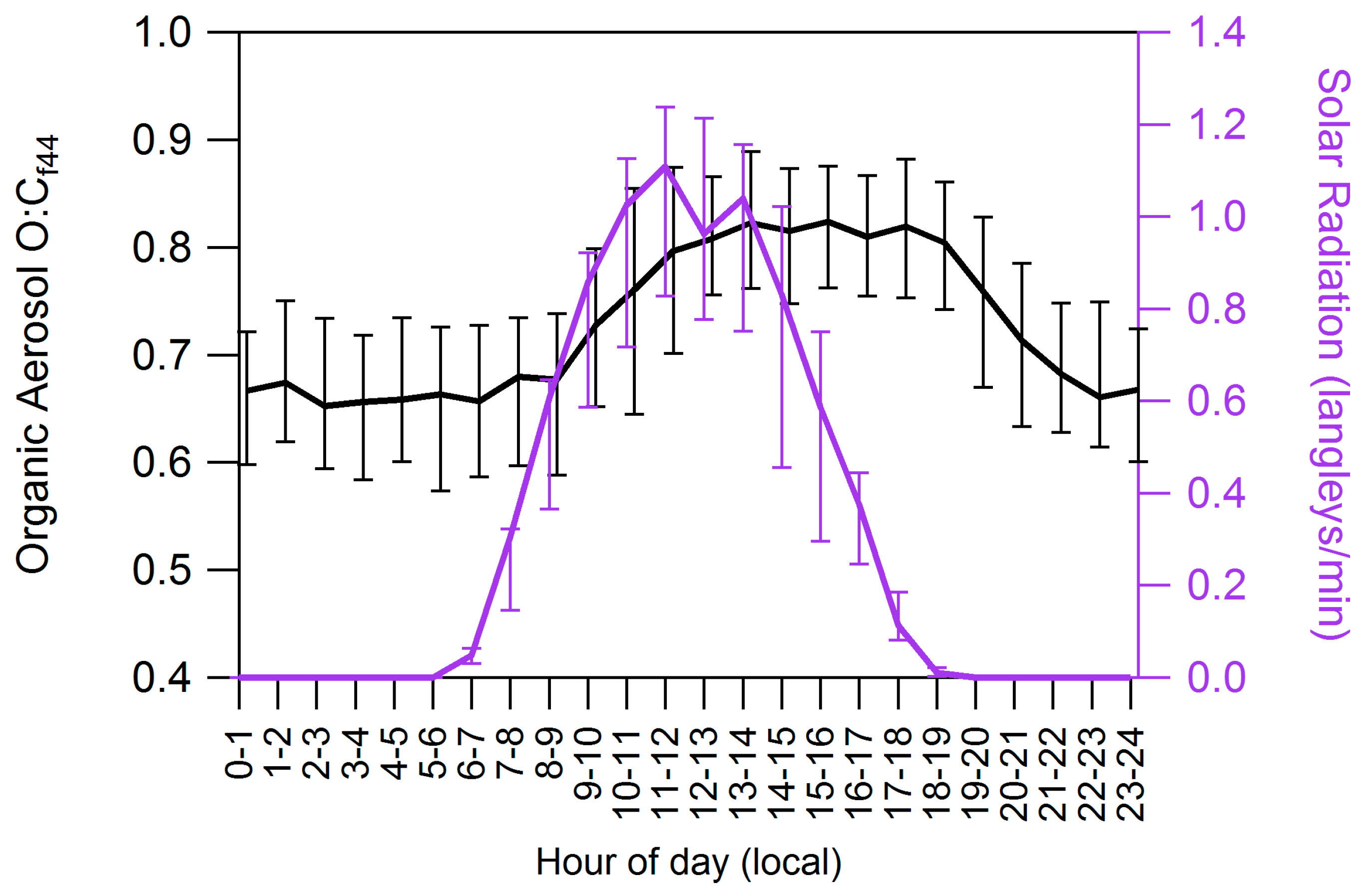
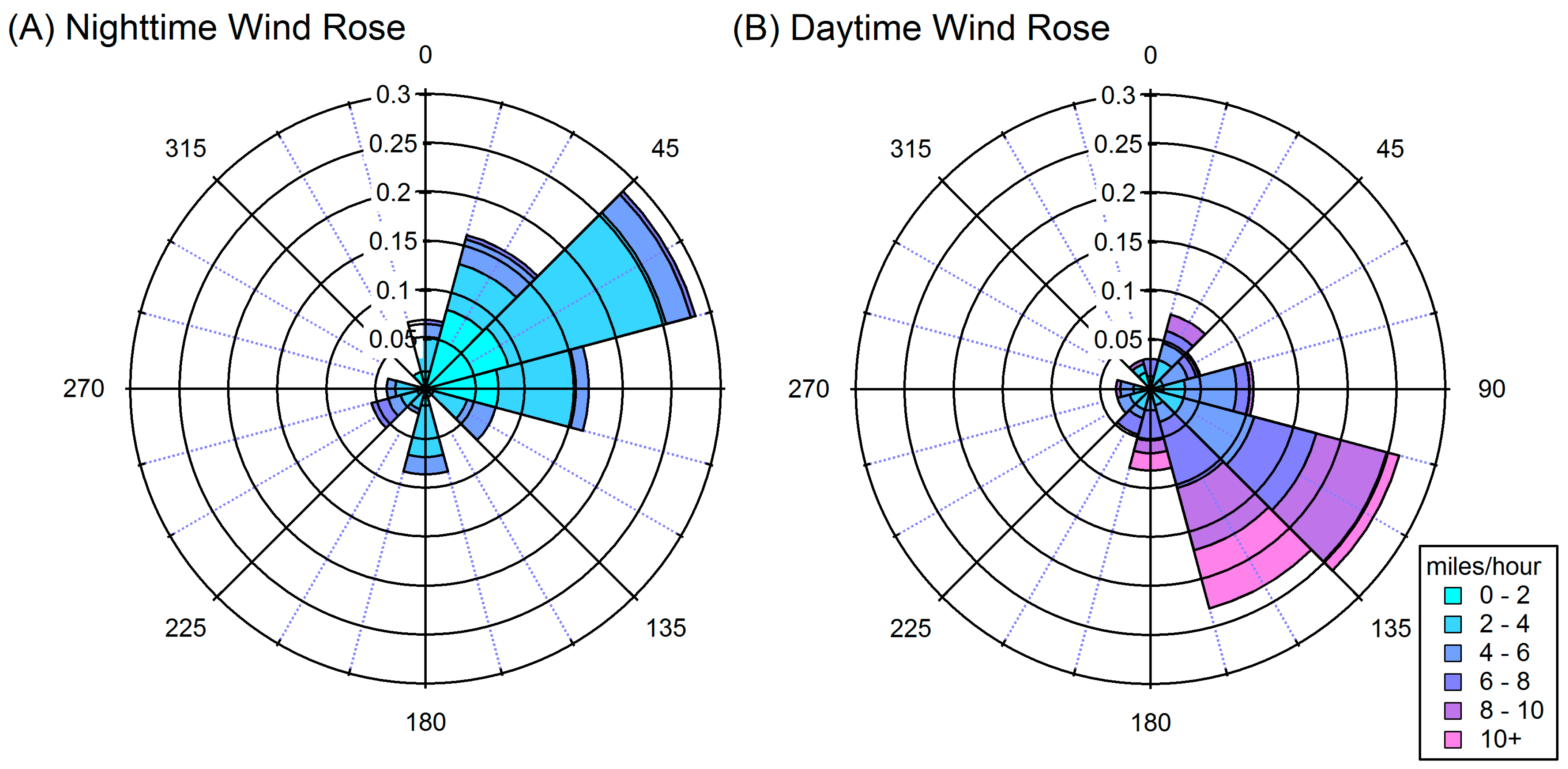
4.2. Influences on Diurnal Cycle

The strong diurnal cycle for organics and nitrate but lack of diurnal cycle for sulfate is consistent with a more regional source of sulfate and a more local source of organics and organic nitrates. The higher amplitude-to-mean ratio of nitrate indicates that the diurnal trend is especially prominent for nitrate and suggests that organic nitrates play a large role in the observed diurnal trends. The more pronounced diurnal changes in organic nitrates could be attributed to evaporation with increasing daytime temperatures or nighttime growth due to NO3 chemistry. NO3, formed from the reaction of NO2 and O3, is considered a night-time oxidant because it photolyzes quickly during the day.
The shape of the diurnal profile shows highest concentrations at night and quick decreases in concentration during daylight hours. Photo-oxidation of organics predominantly decreases their vapor pressure and can result in overall increases of organic particulate matter during the day. The diurnal cycle of the organic aerosol O:C ratio (Figure 7) suggests that organic aerosol is more oxygenated during daylight hours, as expected with increasing photochemical activity. PMF results also support this, as daytime decreases are seen in HOA and LO-OOA, potentially indicating conversion to MO-OOA. However, total organic concentrations also decrease during this time, indicating that photochemical activity is not the main factor affecting concentrations of OA.
Some meteorological factors may play a significant role in diurnal trends. Temperature and boundary layer height (BLH) effects on concentrations of PM are explored in Figure 8. Temperature increases when the sun rises, increasing the saturation vapor pressure of particle-phase compounds which causes the higher vapor-pressure species to evaporate. According to absorptive partitioning theory [54,55], the gas-particle partitioning of an organic species depends on its vapor pressure and the concentration of organic material already in the condensed phase. The fraction of a compound i in the particle phase (Yi) is given by [55]:
Y i = ( 1 + C i * C O A ) 1
where C i * is a function of the vapor pressure, If C i * is known at one temperature then it can be predicted at a second temperature if Δ H v a p is known using the Clausius-Clapeyron equation [48]:
C * ( T 2 ) = C * ( T 1 ) e x p ( Δ H v a p R ( 1 T 1 1 T 2 ) )
In a simplified yet illustrative calculation, we assume that Δ H v a p = 40   k J · m o l 1 [55] and assume an initial set of C i * values of those used by Murphy and Pandis [56] for high-NOx terpene SOA. We assume this set of C i * values applies to the average OA concentration (including both the organics and nitrate measured by the ACSM) measured from 0:00 to 6:00 (the time period when concentrations and temperatures were stable) at the average temperature from 0:00 to 6:00 and then calculate the expected OA concentrations, based on observed temperature changes, for the entire day as seen in Figure 8C. Though these assumptions greatly simplify evaporation behavior of the organic aerosol, it is illustrative to see that the resulting predicted OA concentrations match the observed trend. Temperature is likely to be partially responsible for the observed diurnal cycle.
The effect of BLH on atmospheric mixing may also play a role, and a similar estimate was performed to illustrate the effect this might have. Carbon monoxide (CO) measurements from the TCEQ Jones Forest site (~10 miles southwest of Conroe site) were used for an estimate of mixing effects. The average CO and OA concentrations between 0:00 and 6:00 were used as a baseline, and then this baseline was diluted or concentrated based on the CO concentrations as seen in Figure 8C. The increase in predicted OA from 6–8 a.m. is most likely a reflection of traffic conditions, but otherwise the CO-predicted OA concentrations match the trend of measurements and show the effect that BLH and mixing may have had on daytime concentrations as the air mass was diluted. Tucker et al. [57] observed that BLH effects on pollutant concentrations in the Houston region are complicated and depend on many factors including the location of source air and turbulence levels. The lack of significant diurnal variation of sulfate could suggest that the effect of BLH on observed concentrations is lower than suggested by our analysis, and/or that BLH and daytime oxidation of SO2 leading to sulfate had opposite effects. It is also consistent with a more regional source of sulfate and similar concentrations above and below the boundary layer. Daytime oxidation of organics is also expected to increase concentrations of OA and partially offset the changes due to temperature and BLH. Nonetheless, the shape of the organic aerosol diurnal variation is consistent with changes in either BLH or temperature, and both are potential influences on the observed diurnal trend.
In order to further explore this diurnal trend we considered PM2.5 (TEOM) measurements at four Houston area sites operated by the TCEQ [22]. Figure 9 shows diurnal cycles of PM2.5 measurements averaged over the month of September and January taken at Conroe (Figure 9A, same site as our location), Kingwood (Figure 9B, midway between Conroe and downtown Houston), Clinton (Figure 9C, downtown Houston location), and Fayette County (Figure 9D, a rural Texas location). Figure 9 shows that the diurnal trend observed in Conroe is not specific to that area; similar patterns are observed in all three of the other areas, and use of ANOVA reveals statistically significant variation by time of day at all four of these monitoring sites. A similar trend is seen in the winter at all locations as also shown in Figure 9. This indicates that colder temperatures and shorter daylight hours do not eliminate the trend, though the decrease in PM concentration starts later in the day.
Variation in the hourly averaged PM2.5 concentrations measured at the Conroe location are reasonably well described with first order harmonic analysis, which can explain 54% of the variation in TEOM readings. Only 15%, 14% and 6% of the variation is explained by first-order harmonic analysis for Clinton, Kingwood, and Fayette County, respectively. We estimate the magnitude of the diurnal cycle as (Avghigh − Avglow)/Mean, where Avghigh and Avglow are calculated as the mean of the six highest and lowest concentrations in the diurnal trend, respectively. The magnitude of diurnal variation using this method is 0.57 for Conroe and 0.45, 0.39, and 0.39 for Kingwood, Clinton, and Fayette County, respectively, suggesting that PM2.5 concentrations measured at Conroe exhibited the strongest diurnal cycle. It is notable that neither Clinton, which has the most anthropogenic influence, nor Fayette County, which has the least anthropogenic influence, has the most pronounced diurnal profile. Distance from the coast can affect diurnal temperature patterns, with coastal areas having milder temperature swings. However, TCEQ data show that the Conroe and Fayette County sites have nearly identical diurnal temperature profiles, suggesting that more than temperature is needed to describe the observed diurnal trend in organic aerosol concentrations. The strong diurnal cycle in Conroe may in part be due to the interaction of anthropogenic oxidants with biogenic hydrocarbons. Vegetation type may play a large role in this as the Conroe area is where the ecosystem transforms from prairie and marsh to the piney woods of the US Southeast, which are known to have higher biogenic emissions [58]. Xu et al. [19] saw a similar diurnal pattern for a less oxidized OA factor in PMF analysis from measurements in Alabama and Georgia, places that have a piney woods ecosystem.
Observations from the HR-ToF-CIMS support the hypothesis that biogenic VOCs are an important contributor to the diurnal cycle seen in OA in Conroe. Recent work [19,20] has suggested that monoterpene reactions with the NO3 radical at night are a significant source of SOA. Gas-phase organic nitrates observed during DISCOVER-AQ, which likely formed from monoterpenes (C10), also exhibited a diurnal trend of elevated concentrations at night. Data from the HR-ToF-CIMS in Figure 10 show increased levels of monoterpene organic nitrates at night, the time when monoterpene and NO3 concentrations are typically highest [59]. Increasing concentrations are also seen in the time just after sunrise when monoterpene concentrations are still high and NO concentrations are increasing. Lee et al. [59] observed a similar increase in gas phase concentrations of biogenic organic nitrates in the hours following sunrise in the SOAS campaign.
The SIMPOL.1 model [60] was used to estimate changes in volatility from the oxidation of VOCs. The SIMPOL.1 model predicts vapor pressure based on molecular functional groups and in this case was used to predict changes in vapor pressure to biogenic VOCs due to the addition of nitrate and hydroxyl functional groups. Using Equation (10) and conditions in Conroe we find that α-pinene or β-pinene which have been oxidized to C10H16NO4 would partition less than 1% to the particle phase. C10H16NO5 would partition 11%–25%, and C10H16NO6 would partition 95%–98% to the particle phase. Thus, C10H16NO6 and compounds that are more oxidized are not likely found at high concentrations in the gas phase but may be important components of the particle phase as was observed by Lee et al. [59]. Most oxidized gas-phase hydrocarbons observed with the HR-ToF-CIMS have a diurnal cycle with elevated daytime concentrations due to photochemistry similar to C5H8NO4 shown on Figure 10. C5H8NO4 is likely an isoprene hydroxyl-nitrate that is formed through an isoprene peroxy-radical and NO, a similar mechanism to the early morning formation of monoterpene nitrates but different from the night-time monoterpene nitrate formation mechanism through reaction with NO3. Isoprene nitrates could be partially responsible for the diurnal trend in OA in the region. Though they mostly form during the day when isoprene concentrations are highest, according to the SIMPOL.1 model a compound such as C5H8NO6 would partition 15% to the particle phase during the day but nearly double that (28%) during the night, which would increase total organic nitrate concentrations.

5. Conclusions

Measurements were taken in Conroe, TX during 24 August–1 October, 2013, as part of DISCOVER-AQ. Organic aerosol (OA) was a major component of the measured particulate matter, constituting 64% of PM1, and up to 41% of the measured OA in the region was organic nitrates. Through PMF the OA was divided into three factors: Two factors were classified as OOA—one more oxidized (MO-OOA) and one less (LO-OOA). A third factor, named HOA, had similarities to hydrocarbon-like OA and biomass burning OA. The LO-OOA and the HOA displayed diurnal cycles in which concentrations increased in the evening and decreased in the morning. This pattern was also seen in the bulk ACSM measurements of organics and nitrate. Night-time chemistry between biogenic compounds (isoprene, terpenes) and anthropogenic oxidants (O3, NO3) appears to contribute to this variation. Temperature and changes in boundary layer height also appear to contribute to the trend.
Understanding diurnal and multi-day trends in PM levels is crucial as regions continue to strive to achieve lower PM levels. Both the anthropogenic and biogenic drivers that cause concentrations to fluctuate need to be understood and correctly modeled for policy-makers to make informed decisions about regulations. Decreasing PM formation can be especially challenging in locations such as Conroe, TX where organic aerosol formation appears to be strongly influenced by the interaction of biogenic hydrocarbons and anthropogenic oxidants.

Acknowledgments

This work was financed in part through six grants from the Texas Commission on Environmental Quality (TCEQ), administered by The University of Texas through the Air Quality Research Program (Projects 12-012, 12-032, 13-022, 14-009, 14-024 and 14-029). The contents, findings opinions and conclusions are the work of the authors and do not necessarily represent findings, opinions or conclusions of the TCEQ. The authors would like to thank the US EPA for the loan of the PM2.5 high volume sampler. The authors gratefully acknowledge the NOAA Air Resources Laboratory (ARL) for the provision of the HYSPLIT transport and dispersion model and/or READY website (http://www.ready.noaa.gov) used in this publication.

Author Contributions

Jeffrey Bean, Cameron Faxon, and Lea Hildebrandt Ruiz planned, prepared and conducted the ambient measurements. Jeffrey Bean analyzed the ambient ACSM and SEMS data presented in this work. Under the guidance of Robert Griffin, Yu Jun Leong, Basak Karakurt Cevik, and H. William Wallace operated the HR-ToF-AMS and analyzed the subsequent data. Under the guidance of Rebecca Sheesley and Sascha Usenko, Stephanie Ortiz analyzed the filter samples, which were collected by Jeffrey Bean and Cameron Faxon. Under the guidance of Lea Hildebrandt Ruiz and Manjula Canagaratna, Jeffrey Bean conducted and interpreted PMF. The manuscript was written by Jeffrey Bean with the guidance of Lea Hildebrandt Ruiz.

Conflicts of Interest

The authors declare no financial conflict of interest.

Appendix A: ACSM Calibration and Data Preparation

A1. ACSM Calibration

The nitrate ionization efficiency (IE) of the ACSM, as well as the relative ionization efficiencies (RIEs) of sulfate and ammonium were measured four times between 24 August and 30 September (the time period during which ACSM data were acquired) using dried ammonium nitrate and ammonium sulfate particles with a diameter of 300 nm. The ratio of IE to the MS airbeam (AB) was constant for these calibrations (within noise), so the average IE/AB value of 3.29 × 10⁻¹¹ Hz−1 was used for the whole campaign, and the IE was determined at any point by multiplying IE/AB by the current AB. The RIE of ammonium measured during the IE calibrations ranged from 4.57 to 5.82, and the measured RIE of sulfate ranged from 0.49 to 0.67. The variation in the values appeared random; therefore the average values of 5.02 and 0.57 were used for the entire campaign for ammonium and sulfate, respectively. The flow rate in the ACSM was 100 cm3·min−1. Lens alignment and flow calibrations were performed at the beginning of the campaign.

A2. Adjustments to the Standard Fragmentation Table

The collected data were analyzed using a standard AMS fragmentation table and batch table [29], with a few modifications: The fragmentation patterns of air at m/z 44 (CO2+), m/z 29 (N15N+) and m/z 16 (O+) were evaluated using filter data that were collected continuously throughout the campaign. N15N+ and CO2+ were calculated as constant fractions of the N2+ signal at m/z 28; the calculated fractions were 7.3 × 10⁻³ and 1.2 × 10⁻³ for N15N+ and CO2+, respectively. O+ was calculated as a constant fraction of N+; the calculated ratio was 0.48. The correction for CO2+ from air using the N2+ signal was calculated by averaging the filter measurements throughout the campaign when particle-phase organics were below 1 µg·m−3 in order to avoid interference of organics being interpreted as CO2+ from air. The correction for N15N+ was calculated as an average of all filter data throughout the campaign.

A3. Data Averaging

For bulk composition analysis (organics, sulfate, ammonium, nitrate), every 10 ACSM data points were averaged, resulting in a time resolution of approximately 25 min (including 12.5 min of averaged sample and 12.5 min of averaged filter data), and 1475 data points throughout the campaign. (ACSM measurements were taken 24 August–30 September 2013). The following detection limits were then calculated considering the 12.5 min sample averaging time [24]: 0.440 µg·m−3 (ammonium), 0.229 µg·m−3 (organics), 0.037 µg·m−3 (sulfate), 0.017 µg·m−3 (nitrate). Application of the detection limits resulted in removal of 68% of the ammonium data, no removal of sulfate data, and removal of 0.3% and 0.7% of organics and nitrate data, respectively. A 42-h period (4–5 September) in which the airbeam was abnormally high and a 68-h period (1–3 September) during which the vaporizer temperature was set to 700 °C were also removed. The f44 data were cleaned as follows: first, every five data points were averaged. Then datapoints for which f44 < 0 or f44 > 1 were removed since these are not physically possible. (7 data points were below zero, and 1 data point was above 1). Then, every four data points were averaged again for an overall time resolution of approximately 50 min. Then data were removed for which the signal of organics at m/z 44 (i.e., f44 × org) was below the detection limit of organics for the 25 min averaging time. This resulted in removal of 17% of the final averaged data.

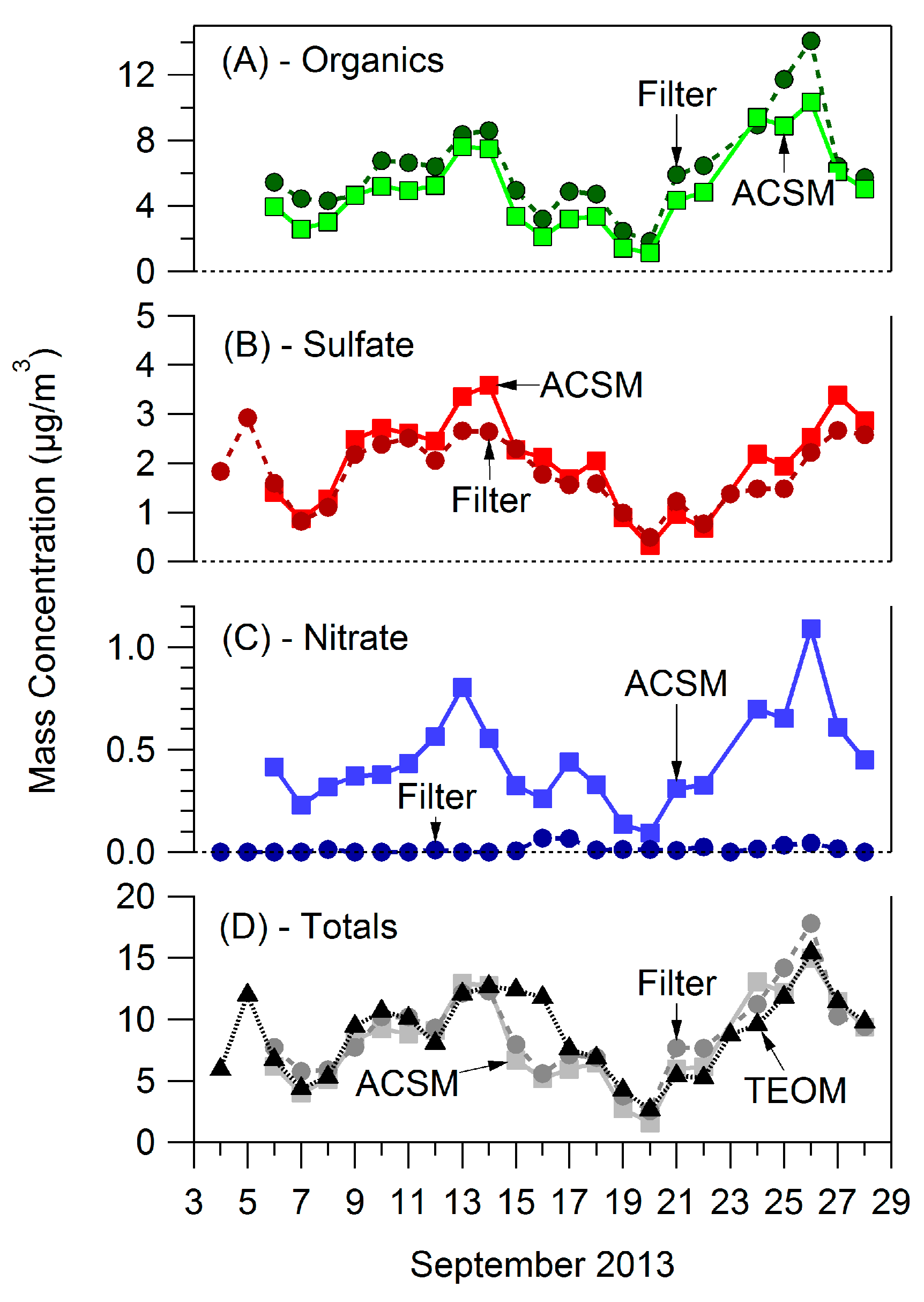
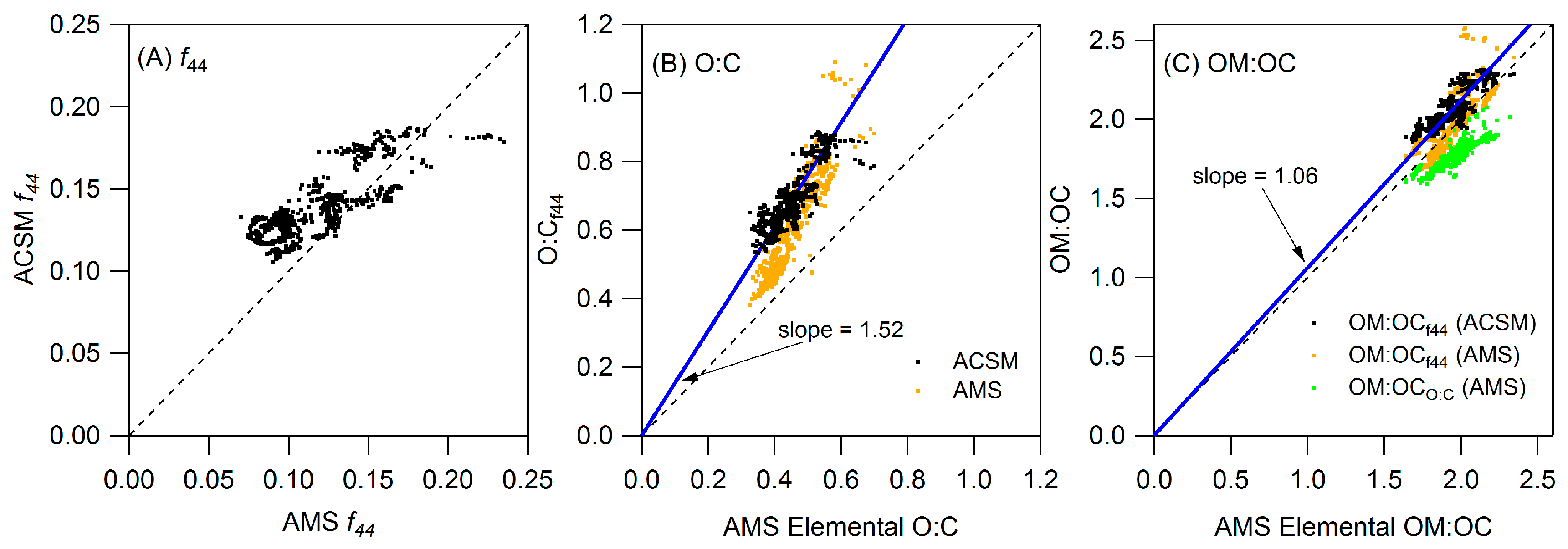
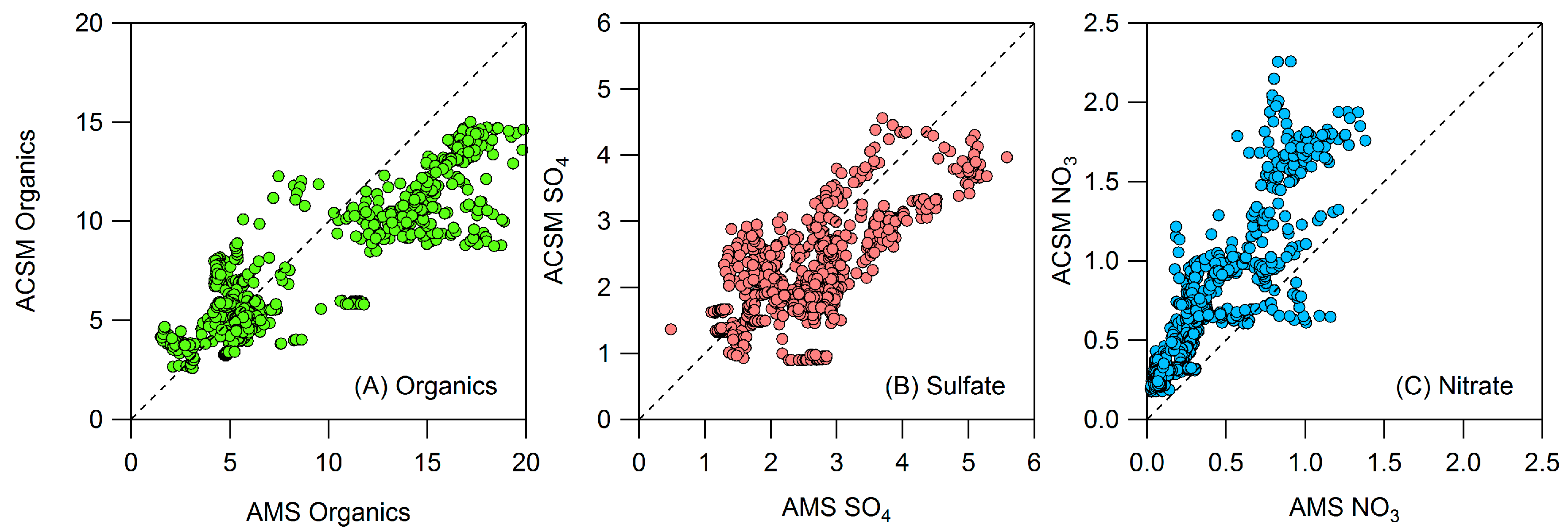
Appendix B: Comparison of Co-Located Instruments

Measurements across different instruments generally agreed throughout the campaign. In Figure A1 we show the comparison between PM1 mass concentrations measured by the ACSM (corrected for CE) and by the SEMS. The volume concentration from the SEMS was converted to mass concentration using the density 1.77 g·cm−3 for ammonium and sulfate and 1.4 g·cm−3 for organics and nitrate [61]. On average the SEMS measured higher PM1 mass (slope = 1.35), which could be due to uncertainties in the density estimate and the SEMS measurement including refractory compounds which are not measured by the ACSM.
Figure A1. Comparison of PM1 mass measured by the SEMS and ACSM throughout the campaign.
Atmosphere 07 00073 g011
Figure A2 compares O:C and OM:OC measurements and estimations by the ACSM and HR-ToF-AMS when the HR-ToF-AMS was at the Conroe site (see Section 2.2.1). There is relatively good agreement in f44 and total organic aerosol mass (Figure A2A and Figure A3A); however, the O:C calculated from measured f44 using Equation (1) (O:Cf44) is significantly higher than the O:C calculated from elemental analysis of the high resolution HR-ToF-AMS spectra (Figure A2B). Despite this difference the calculated OM:OC is similar to the OM:OC from elemental analysis of the co-located HR-ToF-AMS (Figure A2C). This is important as OM:OC is used to convert filter measurements of organic carbon to organic mass (as described below).
Figure A2. Comparison of (A) f44; (B) O:C and (C) OM:OC between the HR-ToF-AMS and ACSM.
Atmosphere 07 00073 g012
ACSM PM1 measurements are also compared with PM2.5 measurements from filter samples (see Section 2.2.4) and the TCEQ-operated TEOM (see Figure A4). The filter measurements of OC are converted to organic mass using the calculated OM:OC ratio described in Section 2.2.1. In general, measurements from the filters are consistent with those from the ACSM, suggesting that the majority of the mass in PM2.5 is found in particles with a diameter below 1 μm (Figure A4A,B,D). The total concentrations from the ACSM and filter measurements are also consistent with the TCEQ-operated TEOM (Figure A4D). The total filter measurement also includes elemental carbon (about 7% of total carbon), which is not measured by the ACSM.
Figure A3. ACSM and HR-ToF-AMS comparison of (A) organics, (B) sulfate, and (C) nitrate. HR-ToF-AMS measurements are high resolution while ACSM measurements are unit mass resolution.
Atmosphere 07 00073 g013
Figure A3 shows that, with the exception of nitrate, speciated measurements between the HR-ToF-AMS (high resolution) and ACSM (unit mass resolution) were reasonably consistent during the times when the HR-ToF-AMS was co-located (61 h over the course of the campaign). Nitrate was measured 60% higher by the ACSM, on average, than by the HR-ToF-AMS. Unit mass resolution measurements of nitrate from the ACSM rely on the standard fragmentation table to estimate the split of m/z 30 between nitrate (NO+) and organics (mostly CH2O+). Conditions with high levels of CH2O+ can result in over-prediction of nitrate by the ACSM. The HR-ToF-AMS directly measures NO+ and CH2O+. In this campaign, the ACSM measurements of nitrate were, on average, 60% higher than the high resolution measurements of nitrate by the HR-ToF-AMS; ACSM measurements were only 20% higher than unit mass resolution measurements by the HR-ToF-AMS, which rely on the same fragmentation table as the ACSM.
Figure A4. Instrument comparisons between the PM1 ACSM, PM2.5 filter, and PM2.5 TEOM measurements for. (A) Organics, (B) Sulfate, (C) Nitrate, (D) Totals.
Atmosphere 07 00073 g014

References

  1. Lim, S.S.; Vos, T.; Flaxman, A.D.; Danaei, G.; Shibuya, K.; Adair-Rohani, H.; Amann, M.; Anderson, H.R.; Andrews, K.G.; Aryee, M.; et al. A comparative risk assessment of burden of disease and injury attributable to 67 risk factors and risk factor clusters in 21 regions, 1990–2010: A systematic analysis for the Global Burden of Disease Study 2010. Lancet 2012, 380, 2224–2260. [Google Scholar] [CrossRef]
  2. Dockery, D.; Pope, C.A.; Xiping, X.; Spengler, J.D.; Ware, J.H.; Fay, M.E.; Ferris, B.G.; Speizer, F.E. An association between air pollution and mortality in six USA cities. N. Engl. J. Med. 1993, 329, 1753–1759. [Google Scholar] [CrossRef] [PubMed]
  3. Tong, D.Q.; Yu, S.; Kan, H. Ozone exposure and mortality. N. Engl. J. Med. 2009, 360, 2788–2789. [Google Scholar] [PubMed]
  4. NAAQS Table. Available online: https://www.epa.gov/criteria-air-pollutants/naaqs-table (accessed on 26 February 2016).
  5. United States Environmental Protection Agency. National Ambient Air Quality Standards for Particulate Matter. Fed. Reg. 2013, 78, 3085–3287. [Google Scholar]
  6. United States Environmental Protection Agency. National Ambient Air Quality Standards for Ozone. Fed. Reg. 2015, 80, 75233–75411. [Google Scholar]
  7. Allen, D.T.; McDonald-Buller, E.C.; McGaughey, G.R. State of the Science of Air Quality in Texas: Scientific Findings from the Air Quality Research Program (AQRP) and Recommendations for Future Research; Air Quality Research Program: Austin, TX, USA, 2016. [Google Scholar]
  8. Allen, D.; Estes, M.; Smith, J.; Jeffries, H. Accelerated Science Evaluation of Ozone Formation in the Houston-Galveston Area; University of Texas: Austin, TX, USA, 2001. [Google Scholar]
  9. Allen, D.T.; Fraser, M. An overview of the gulf coast aerosol research and characterization study: The Houston fine particulate matter supersite. J. Air Waste Manag. Assoc. 2006, 56, 456–466. [Google Scholar] [CrossRef] [PubMed]
  10. Olaguer, E.; Kolb, C.; Lefer, B.; Rappenglueck, B.; Zhang, R.; Pinto, J. Overview of the SHARP campaign: Motivation, design, and major outcomes. J. Geophys. Res. Atmos. 2014, 119, 2597–2610. [Google Scholar] [CrossRef]
  11. Allen, D.T.; Torres, V.M.; Thomas, J.; Sullivan, D.W.; Harrison, M.; Hendler, A.; Herndon, S.C.; Kolb, C.E.; Fraser, M.P.; Hill, A.D.; et al. Measurements of methane emissions at natural gas production sites in the United States. Proc. Natl. Acad. Sci. USA 2013, 110, 17768–17773. [Google Scholar] [CrossRef] [PubMed]
  12. Pasci, A.; Kimura, Y.; McGaughey, G.; McDonald-Buller, E.; Allen, D.T. Regional ozone impacts of increased natural gas use in the Texas power sector and development in the Eagle Ford shale. Environ. Sci. Technol. 2015, 49, 3966–3973. [Google Scholar]
  13. Zavala-Araiza, D.; Sullivan, D.W.; Allen, D.T. Atmospheric hydrocarbon emissions and concentrations in the Barnett Shale natural gas production region. Environ. Sci. Technol. 2014, 48, 5314–5321. [Google Scholar] [CrossRef] [PubMed]
  14. Bahreini, R.; Ervens, B.; Middlebrook, A.M.; Warneke, C.; de Gouw, J.A.; DeCarlo, P.F.; Jimenez, J.L.; Brock, C.A.; Neuman, J.A.; Ryerson, T.B.; et al. Organic aerosol formation in urban and industrial plumes near Houston and Dallas, Texas. J. Geophys. Res. Atmos. 2009, 114, 1–17. [Google Scholar] [CrossRef]
  15. Murphy, B.N.; Donahue, N.M.; Robinson, A.L.; Pandis, S.N. A naming convention for atmospheric organic aerosol. Atmos. Chem. Phys. 2014, 14, 5825–5839. [Google Scholar] [CrossRef] [Green Version]
  16. Parrish, D.D.; Allen, D.T.; Bates, T.S.; Estes, M.; Fehsenfeld, F.C.; Feingold, G.; Ferrare, R.; Hardesty, R.M.; Meagher, J.F.; Nielsen-Gammon, J.W.; et al. Overview of the second texas air quality study (TexAQS II) and the Gulf of Mexico atmospheric composition and climate study (GoMACCS). J. Geophys. Res. Atmos. 2009, 114, 1–28. [Google Scholar] [CrossRef]
  17. Weber, R.; Sullivan, A.; Peltier, R.; Russell, A.; Yan, B.; Zheng, M.; de Gouw, J.; Warneke, C.; Brock, C.; Holloway, J.; et al. A study of secondary organic aerosol formation in the anthropogenic-influenced southeastern United States. J. Geophys. Res. Atmos. 2007, 112. [Google Scholar] [CrossRef]
  18. Xu, L.; Guo, H.; Boyd, C.M.; Bougiatioti, A.; Cerully, K.M.; Hite, J.R.; Isaacman-Vanwertz, G.; Kreisberg, N.M.; Olson, K.; Koss, A.; et al. Effects of anthropogenic emissions on aerosol formation from isoprene and monoterpenes in the southeastern United States. Proc. Natl. Acad. Sci. USA 2015, 112, 37–42. [Google Scholar] [CrossRef] [PubMed]
  19. Xu, L.; Suresh, S.; Guo, H.; Weber, R.J.; Ng, N.L. Aerosol characterization over the southeastern United States using high-resolution aerosol mass spectrometry: Spatial and seasonal variation of aerosol composition and sources with a focus on organic nitrates. Atmos. Chem. Phys. 2015, 15, 7307–7336. [Google Scholar] [CrossRef]
  20. Boyd, C.M.; Sanchez, J.; Xu, L.; Eugene, A.J.; Nah, T.; Tuet, W.Y.; Guzman, M.I.; Ng, N.L. Secondary organic aerosol formation from the β-pinene+NO3 system: Effect of humidity and peroxy radical fate. Atmos. Chem. Phys. 2015, 15, 7497–7522. [Google Scholar] [CrossRef]
  21. DISCOVER-AQ Home. Available online: http://discover-aq.larc.nasa.gov/ (accessed on 26 February 2016).
  22. Texas Air Monitoring Information System (TAMIS) Web Interface. Available online: http://www17.tceq.texas.gov/tamis/ (accessed on 26 February 2016).
  23. Kebabian, P.L.; Wood, E.C.; Herndon, S.C.; Freedman, A. A Practical Alternative to Detection of Nitrogen Dioxide: Cavity Attenuated Phase Shift Spectroscopy. Environ. Sci. Technol. 2008, 42, 6040–6045. [Google Scholar] [CrossRef] [PubMed]
  24. Ng, N.L.; Herndon, S.C.; Trimborn, A.; Canagaratna, M.R.; Croteau, P.L.; Onasch, T.B.; Sueper, D.; Worsnop, D.R.; Zhang, Q.; Sun, Y.L.; et al. An Aerosol Chemical Speciation Monitor (ACSM) for routine monitoring of the composition and mass concentrations of ambient aerosol. Aerosol Sci. Technol. 2011, 45, 780–794. [Google Scholar] [CrossRef]
  25. Bertram, T.H.; Kimmel, J.R.; Crisp, T.A.; Ryder, O.S.; Yatavelli, R.L.N.; Thornton, J.A.; Cubison, M.J.; Gonin, M.; Worsnop, D.R. A field-deployable, chemical ionization time-of-flight mass spectrometer. Atmos. Meas. Tech. 2011, 4, 1471–1479. [Google Scholar] [CrossRef]
  26. Yatavelli, R.L.N.; Lopez-Hilfiker, F.; Wargo, J.D.; Kimmel, J.R.; Cubison, M.J.; Bertram, T.H.; Jimenez, J.L.; Gonin, M.; Worsnop, D.R.; Thornton, J.A. A chemical ionization high-resolution time-of-flight mass spectrometer coupled to a Micro Orifice Volatilization Impactor (MOVI-HRToF-CIMS) for analysis of gas and particle-phase organic species. Aerosol Sci. Technol. 2012, 46, 1313–1327. [Google Scholar] [CrossRef]
  27. Lee, B.H.; Lopez-Hilfiker, F.D.; Mohr, C.; Kurtén, T.; Worsnop, D.R.; Thornton, J.A. An iodide-adduct high-resolution time-of-flight chemical-ionization mass spectrometer: Application to atmospheric inorganic and organic compounds. Environ. Sci. Technol. 2014, 48, 6309–6317. [Google Scholar] [CrossRef] [PubMed]
  28. Aljawhary, D.; Lee, A.K.Y.; Abbatt, J.P.D. High-resolution chemical ionization mass spectrometry (ToF-CIMS): Application to study SOA composition and processing. Atmos. Meas. Tech. 2013, 6, 3211–3224. [Google Scholar] [CrossRef]
  29. Allan, J.D.; Delia, A.E.; Coe, H.; Bower, K.N.; Alfarra, M.R.; Jimenez, J.L.; Middlebrook, A.M.; Drewnick, F.; Onasch, T.B.; Canagaratna, M.R.; et al. A generalised method for the extraction of chemically resolved mass spectra from Aerodyne aerosol mass spectrometer data. J. Aerosol Sci. 2004, 35, 909–922. [Google Scholar] [CrossRef]
  30. Leong, Y.J.; Sanchez, N.P.; Wallace, H.W.; Karakurt Cevik, B.; Hernandez, C.S.; Han, Y.; Choi, Y.; Flynn, J.H.; Massoli, P.; Floerchinger, C.; et al. Overview of Surface Measurements and Spatial Characterization of Submicron Particulate Matter during the DISCOVER-AQ 2013 Campaign in Houston, TX, USA, 2016. in preparation.
  31. Aiken, A.C.; Decarlo, P.F.; Kroll, J.H.; Worsnop, D.R.; Huffman, J.A.; Docherty, K.S.; Ulbrich, I.M.; Mohr, C.; Kimmel, J.R.; Sueper, D.; et al. O/C and OM/OC Ratios of primary, secondary, and ambient organic aerosols with high-resolution time-of-flight aerosol mass spectrometry. Environ. Sci. Technol. 2008, 42, 4478–4485. [Google Scholar] [CrossRef] [PubMed]
  32. Canagaratna, M.R.; Jimenez, J.L.; Kroll, J.H.; Chen, Q.; Kessler, S.H.; Massoli, P.; Hildebrandt Ruiz, L.; Fortner, E.; Williams, L.R.; Wilson, K.R.; et al. Elemental ratio measurements of organic compounds using aerosol mass spectrometry: Characterization, improved calibration, and implications. Atmos. Chem. Phys. 2015, 15, 253–272. [Google Scholar] [CrossRef]
  33. Paatero, P.; Tapper, U. Positive matrix factorization: A nonnegative factor model with optimal utilization of error estimates of data values. Environmetrics 1994, 5, 111–126. [Google Scholar] [CrossRef]
  34. Hildebrandt, L.; Engelhart, G.J.; Mohr, C.; Kostenidou, E.; Lanz, V.A.; Bougiatioti, A.; DeCarlo, P.F.; Prevot, A.S.H.; Baltensperger, U.; Mihalopoulos, N.; et al. Aged organic aerosol in the eastern Mediterranean: The finokalia aerosol measurement experiment–2008. Atmos. Chem. Phys. 2010, 10, 4167–4186. [Google Scholar] [CrossRef]
  35. Hildebrandt, L.; Kostenidou, E.; Lanz, V.A.; Prevot, A.S.H.; Baltensperger, U.; Mihalopoulos, N.; Donahue, N.M.; Pandis, S.N. Sources and atmospheric processing of organic aerosol in the Mediterranean: Insights from aerosol mass spectrometer factor analysis. Atmos. Chem. Phys. 2011, 11, 12499–12515. [Google Scholar] [CrossRef]
  36. Lanz, V.A.; Alfarra, M.R.; Baltensperger, U.; Buchmann, B.; Hueglin, C.; Prevot, A.S.H. Source apportionment of submicron organic aerosols at an urban site by factor analytical modelling of aerosol mass spectra. Atmos. Chem. Phys. 2007, 7, 1503–1522. [Google Scholar] [CrossRef]
  37. Lanz, V.A.; Prévôt, A.S.H.; Alfarra, M.R.; Weimer, S.; Mohr, C.; DeCarlo, P.F.; Gianini, M.F.D.; Hueglin, C.; Schneider, J.; Favez, O.; et al. Characterization of aerosol chemical composition with aerosol mass spectrometry in Central Europe: An overview. Atmos. Chem. Phys. 2010, 10, 10453–10471. [Google Scholar] [CrossRef]
  38. Ulbrich, I.M.; Canagaratna, M.R.; Zhang, Q.; Worsnop, D.R.; Jimenez, J.L. Interpretation of organic components from Positive Matrix Factorization of aerosol mass spectrometric data. Atmos. Chem. Phys. 2009, 9, 2891–2918. [Google Scholar] [CrossRef]
  39. Faxon, C.; Bean, J.; Hildebrandt Ruiz, L. Inland concentrations of ClNO2 in Southeast Texas suggest chlorine chemistry significantly contributes to atmospheric reactivity. Atmosphere 2015, 6, 1487–1506. [Google Scholar] [CrossRef]
  40. Birch, M.; Cary, R. Elemental carbon-based method for monitoring occupational exposures to particulate diesel exhaust. Aerosol Sci. Technol. 1996, 25, 221–241. [Google Scholar] [CrossRef]
  41. Zaveri, R.A.; Shaw, W.J.; Cziczo, D.J.; Schmid, B.; Ferrare, R.A.; Alexander, M.L.; Alexandrov, M.; Alvarez, R.J.; Arnott, W.P.; Atkinson, D.B.; et al. Overview of the 2010 Carbonaceous Aerosols and Radiative Effects Study (CARES). Atmos. Chem. Phys. 2012, 12, 7647–7687. [Google Scholar] [CrossRef] [Green Version]
  42. Zotter, P.; El-Haddad, I.; Zhang, Y.; Hayes, P.L.; Zhang, X.; Lin, Y.; Wacker, L.; Schnelle-Kreis, J.; Abbaszade, G.; Zimmermann, R.; et al. Diurnal cycle of fossil and nonfossil carbon using radiocarbon analyses during CalNex. J. Geophys. Res. Atmos. 2014, 119, 6818–6835. [Google Scholar] [CrossRef]
  43. Barrett, T.E.; Robinson, E.M.; Usenko, S.; Sheesley, R.J. Source contributions to wintertime elemental and organic carbon in the western arctic based on radiocarbon and tracer apportionment. Environ. Sci. Technol. 2015, 49, 11631–11639. [Google Scholar] [CrossRef] [PubMed]
  44. Gustafsson, Ö.; Kruså, M.; Zencak, Z.; Sheesley, R.J.; Granat, L.; Engström, E.; Praveen, P.S.; Rao, P.S.P.; Leck, C.; Rodhe, H. Brown clouds over South Asia: Biomass or fossil fuel combustion? Science 2009, 323, 495–498. [Google Scholar] [CrossRef] [PubMed]
  45. Atkinson-Palombo, C.M.; Miller, J.A.; Balling, R.C., Jr. Quantifying the ozone “weekend effect” at various locations in Phoenix, Arizona. Atmos. Environ. 2006, 40, 7644–7658. [Google Scholar] [CrossRef]
  46. Wilks, D.S. Statistical Methods in the Atmospheric Science; Academic Press: San Diego, CA, USA, 1995. [Google Scholar]
  47. Ng, N.L.; Canagaratna, M.R.; Jimenez, J.L.; Zhang, Q.; Ulbrich, I.M.; Worsnop, D.R. Real-time methods for estimating organic component mass concentrations from aerosol mass spectrometer data. Environ. Sci. Technol. 2011, 45, 910–916. [Google Scholar] [CrossRef] [PubMed]
  48. Rollins, A.W.; Browne, E.C.; Min, K.-E.; Pusede, S.E.; Wooldridge, P.J.; Gentner, D.R.; Goldstein, A.H.; Liu, S.; Day, D.A.; Russell, L.M.; et al. Evidence for NOx control over nighttime SOA formation. Science 2012, 337, 1210–1212. [Google Scholar] [CrossRef] [PubMed]
  49. Mylonas, D.T.; Allen, D.T.; Ehrmanf, S.H.; Pratsins, S.E. The sources and size distributions of organonitrates in Los Angeles aerosol. Atmos. Environ. 1991, 25A, 2855–2861. [Google Scholar] [CrossRef]
  50. Garnes, L.A.; Allen, D.T. Size distributions of organonitrates in ambient aerosol collected in Houston, Texas. Aerosol Sci. Technol. 2002, 36, 983–992. [Google Scholar] [CrossRef]
  51. Laurent, J.-P.; Allen, D.T. Size distributions of organic functional groups in ambient aerosol collected in Houston, Texas. Aerosol Sci. Technol. 2004, 38, 60–67. [Google Scholar] [CrossRef]
  52. O’Brien, R.J.; Holmes, J.R.; Bockian, A.H. Formation of photochemical aerosol from hydrocarbons. chemical reactivity and products. Environ. Sci. Technol. 1975, 9, 568–576. [Google Scholar] [CrossRef]
  53. Stein, A.F.; Draxler, R.R.; Rolph, G.D.; Stunder, B.J.B.; Cohen, M.D.; Ngan, F. NOAA’S HYSPLIT atmospheric transport and dispersion modeling system. Am. Meteorol. Soc. 2015, 96, 2059–2077. [Google Scholar] [CrossRef]
  54. Pankow, J.F. An absorption model of gas/particle partitioning of organic compounds in the atmosphere. Atmos. Environ. 1994, 28, 185–188. [Google Scholar] [CrossRef]
  55. Donahue, N.M.; Robinson, A.L.; Stanier, C.O.; Pandis, S.N. Coupled partitioning, dilution, and chemical aging of semivolatile organics. Environ. Sci. Technol. 2006, 40, 2635–2643. [Google Scholar] [CrossRef] [PubMed]
  56. Murphy, B.N.; Pandis, S.N. Exploring summertime organic aerosol formation in the eastern United States using a regional-scale budget approach and ambient measurements. J. Geophys. Res. 2010, 115, D24216. [Google Scholar] [CrossRef]
  57. Tucker, S.C.; Banta, R.M.; Langford, A.O.; Senff, C.J.; Brewer, W.A.; Williams, E.J.; Lerner, B.M.; Osthoff, H.D.; Hardesty, R.M. Relationships of coastal nocturnal boundary layer winds and turbulence to Houston ozone concentrations during TexAQS 2006. J. Geophys. Res. 2010, 115, 1–17. [Google Scholar] [CrossRef]
  58. Vizuete, W.; Junquera, V.; McDonald-Buller, E.; McGaughey, G.; Yarwood, G.; Allen, D. Effects of temperature and land use on predictions of biogenic emissions in Eastern Texas, USA. Atmos. Environ. 2002, 36, 3321–3337. [Google Scholar] [CrossRef]
  59. Lee, B.H.; Mohr, C.; Lopez-Hilfiker, F.D.; Lutz, A.; Hallquist, M.; Lee, L.; Romer, P.; Cohen, R.C.; Iyer, S.; Kurtén, T.; et al. Highly functionalized organic nitrates in the southeast United States: Contribution to secondary organic aerosol and reactive nitrogen budgets. Proc. Natl. Acad. Sci. USA 2016, 113, 1516–1521. [Google Scholar] [CrossRef] [PubMed]
  60. Pankow, J.F.; Asher, W.E. SIMPOL.1: A simple group contribution method for predicting vapor pressures and enthalpies of vaporization of multifunctional organic compounds. Atmos. Chem. Phys. 2008, 8, 2773–2796. [Google Scholar] [CrossRef]
  61. Ng, N.L.; Chhabra, P.S.; Chan, A.W.H.; Surratt, J.D.; Kroll, J.H.; Kwan, A.J.; McCabe, D.C.; Wennberg, P.O.; Sorooshian, A.; Murphy, S.M.; et al. Effect of NOx level on secondary organic aerosol (SOA) formation from the photooxidation of terpenes. Atmos. Chem. Phys. Discuss. 2007, 7, 10131–10177. [Google Scholar] [CrossRef]
Figure 1. Campaign measurements from ACSM, SEMS.
Atmosphere 07 00073 g001
Figure 2. (AC) Diurnal plots for organics, nitrate, and sulfate measured by the ACSM; (D) PM1 measured by the SEMS. Median values are plotted, with error bars showing the 25th and 75th percentiles.
Atmosphere 07 00073 g002
Figure 3. Mass spectra (left) and diurnal profiles (right) of PMF factors.
Atmosphere 07 00073 g003
Figure 4. Time series of PMF factors in terms of fractional concentrations.
Atmosphere 07 00073 g004
Figure 5. HYSPLIT 72-h back trajectories showing the differences between lower (A) and higher (B) concentration days. The low and high trajectories correspond to 2:00, 8 September and 2:00 26 September, respectively. Seventy-two-hour back trajectories are also shown for 14:00 26 September (C), so (B,C) show a typical 12 h difference.
Atmosphere 07 00073 g005
Figure 6. Wind rose plots for (A) night (0:00–6:00) and (B) day (12:00–18:00) averaged over the course of the campaign.
Atmosphere 07 00073 g006
Figure 7. Diurnal cycle of organic aerosol oxygen to carbon ratio (O:Cf44) and solar radiation.
Atmosphere 07 00073 g007
Figure 8. Diurnal profiles of (A) temperature and (B) carbon monoxide. (C) shows the diurnal profile of OA as well as the diurnal profile of OA predicted by temperature and boundary layer height changes. Starting concentrations in predictions are the average of measured concentrations between 0:00 and 6:00.
Atmosphere 07 00073 g008
Figure 9. Diurnal plots for Conroe and neighboring areas based on tapered element oscillating microbalance (TEOM) measurements of PM2.5 by the Texas Commission on Environmental Quality (TCEQ). (A) Conroe, (B) Kingwood, (C) Clinton, (D) Fayette County.
Atmosphere 07 00073 g009
Figure 10. Diurnal plot of gas-phase organic nitrates which appear to have formed from biogenic compounds. These HR-ToF-CIMS data are taken from the high-concentration period of 11–14 September.
Atmosphere 07 00073 g010

