Article

Impacts of Soil Moisture on Typical Frontal Rainstorm in Yangtze River Basin

1
Collaborative Innovation Center on Forecast and Evaluation of Meteorological Disasters, Nanjing University of Information Science and Technology, Nanjing 210044, China
2
Key Laboratory of Meteorological Disaster of Ministry of Education, Nanjing University of Information Science and Technology, Nanjing 210044, China
3
Department of Atmospheric Science, Nanjing University of Information Science and Technology, Nanjing 210044, China
4
Department of Geography and Remote Sensing, Nanjing University of Information Science and Technology, Nanjing 210044, China
*
Author to whom correspondence should be addressed.
Atmosphere 2016, 7(3), 42; https://doi.org/10.3390/atmos7030042
Submission received: 20 January 2016 / Revised: 25 February 2016 / Accepted: 26 February 2016 / Published: 11 March 2016

Abstract

:
By using a coupled land surface-atmosphere model with initial conditions of varying resolution and ensembles of systematically changed soil moisture, convective-scale simulations of a typical frontal rainstorm in the Yangtze River Basin are collected to investigate: (1) effects of different datasets on the simulated frontal mesoscale convective systems (MCSs); (2) possible linkages between soil moisture, planetary boundary layer (PBL), MCSs and precipitation in this modeled rainstorm. Firstly, initial soil moisture differences can affect the PBL, MCSs and precipitation of this frontal rainstorm. Specially, for a 90 mm precipitation forecast, the Threat score (TS) can increase 6.61% by using the Global Land Data Assimilation System (GLDAS) soil moisture. Secondly, sensitivity experiment results show that the near-surface thermodynamic conditions are more sensitive to dry soil than wet due to the initial moist surface; atmosphere conditions have suppressed the relations between soil and atmosphere; and decreased precipitation can be found over both wet and dry surfaces. Generally, a positive feedback between soil moisture and the near-surface thermodynamic conditions is identified, while the relations between soil moisture and precipitation are quite complicated. This relationship shows a daytime mixing of warm surface soil over dry surfaces and a daytime evaporation of adequate moisture over wet surfaces. The large-scale forcing can affect these relations and finally cause decreased precipitation over both wet and dry surfaces.

1. Introduction

Soil moisture has been widely recognized as one of the key factors for rainfall prediction [1,2,3,4,5,6]. The relationship between soil moisture and precipitation is typically described as a closed feedback loop [7,8,9]. This feedback has been verified by many observational and numerical studies in the transition zones between dry and wet climatic regions, where the high coupling between the land surface and the planetary boundary layer (PBL) could significantly influence the mesoscale convective systems (MCSs) [10,11]. In climate scales, positive effects of soil moisture on atmosphere in this closed feedback loop are suggested as the following: soil moisture partitions available net radiation into latent heat for evapotranspiration and sensible heat for temperature increase [12,13,14,15,16]. Therefore, soil moisture controls, to some extent, the thermodynamic conditions of the overlying lower atmosphere, which alters the PBL depth and moist static energy (MSE), and thus ultimately modulates the convective activities of the upper layers [8,9]. Especially, a decrease in soil moisture may actually increase the clouds of the PBL in several observational cases [17,18], which has supported the negative relations between land surface moisture and its overlaying atmosphere. Additionally, these interactions between the shallow cumulus of the PBL and the land surface moisture can further regulate these large-scale effects [19].
The effects of soil moisture on atmosphere are found to be relevant at a variety of spatial and temporal scales [8,20,21]. In convective scales, it has been found that soil moisture can notably influence the precipitation [10]; however, these effects are mostly modulated by the surface variability [22] and atmosphere conditions. The well-known sea-breeze-like circulation [23,24], induced by horizontal variations of surface fluxes, could favor deep convections [25]. Although such thermal circulations are not easy to capture in realistic weather [26], they have been verified by several observational studies [27,28] and further reported in a high resolution simulation of a fair weather with the Weather Research and Forecasting (WRF) model [29]. Recently, several studies have suggested that surface variability could trigger the overlying convective activities [30,31,32], and this inhomogeneous surface could affect the pathways and intensity of deep convections [11,33]; in addition, other studies have suggested that the mid-layer background winds could exert an influence of the MCSs over this surface variability [34,35]. Generally, these convective-scale effects could govern the ways of the aforementioned large-scale feedbacks.
As the linkages between PBL cumulus and land surface moisture in these effects are complicated by the thermodynamic conditions and environmental winds [19], earlier observational work has reported the atmospheric conditions largely determining both the negative and the positive effects of homogeneous surfaces on MCSs by using a measurement based on the low-level temperature and humidity to identify the favorable or unfavorable atmospheric conditions in soil-atmosphere interactions [20]. Several numerical studies have further pointed out that a weak forcing atmosphere can promise a high coupling between soil moisture and atmosphere in convective-scale simulations [36,37,38]. However, it has been reported that these effects in convective scales are mostly decided by the model resolutions because of imperfect model physics [29,39], and even different models within the same initial conditions have been shown to simulate these effects [40].
In the Yangtze River Basin, observational studies have reported that the correlations between soil moisture and atmosphere are notably positive in precipitation and negative in the near-surface temperature [41]. These relationships are relatively significant during the local summertime [42]. Several numerical studies have verified this significant effect of soil moisture on low-level atmosphere in the summer [43,44,45,46]. Zhang et al. [47] have studied the contributions of land-atmosphere coupling to the inter-annual variability of the summer climate by using the WRF model and pointed out this coupling is likely determined by other physical processes besides surface conditions. Li et al. [48], however, have simulated weak correlations between soil moisture and precipitation over East Asia by using the coupled atmospheric general circulation model (AGCM) and inter-annually varying soil moisture. However, the mechanism of the interactions between soil moisture and PBL variables is still unknown, and the relationship between soil moisture and precipitation in this region is still argued about the unfavorable atmosphere and moist surface [47,49]. Regional climate model simulations employed over sub-seasonal or greater time scales are exposed to uncertainty in the linkages among land surface effects, the PBL, and the precipitation that arise from the necessary use of model physics, in which closure assumptions that affect convection initiation are quite varied [39].
The main objective in this study is to understand how the land surface might influence the typical frontal rainstorm embedded in the summer monsoon. Firstly, the effect of soil moisture on the frontally convective-scale characteristics in the Yangtze River Basin is an important topic in this study. As resolution and specificity of initial land surface conditions are crucial in simulating the interactions between the land surface and atmosphere in convective scales [50], several studies have suggested large biases of surface variables [51,52] in the climatic reanalysis over the Yangtze River Basin. Secondly, in order to obtain the realistic soil-atmosphere relations, the effects of three different datasets on this convective-scale simulation are primarily identified by being compared to the observed rainstorm. The current study applies a different approach to analyzing the sensitivity of the PBL and precipitation to land surface conditions, which can help us understand the local land surface effects on typical frontal convection development.
In the Yangtze River Basin, many previous studies that concentrated on the sub-seasonal or inter-annual scales were incapable of identifying the gaps in the spatial and temporal scales. Our study which employs a high resolution simulation with a short time period will broaden our understandings in the convective-scale soil-atmosphere interactions and can enhance our knowledge in the model forecast resulting from different datasets. This could improve numerical weather prediction, which is quite important for agricultural irrigation management [53,54,55,56].

2. Simulation Description

2.1. Model and Data

The model used for this study is the Advanced Research WRF (ARW version 3) described by Skamarock et al. [57], coupled with the Unified Noah Land Surface Model (Noah LSM), as described by Chen and Duhia [58]. The Noah LSM contains four soil layers at depths of 10 cm, 30 cm, 60 cm and 100 cm, within a canopy surface and a deep root zone layer. Two one-way nested domains are employed, centered at Nanjing (32.0°N, 118.5°E), with the horizontal grid spacings of 12 km and 4 km, respectively (Figure 1). Our choices of domain size and grid spacing reflect a compromise that allows us to assess effects of surface conditions on the PBL and isolated MCSs over a relatively small region. Each domain has 50 vertical levels, among which 21 layers under a 5-km model height are selected to study the boundary layer characteristics; the bottom model layer is about at 35–45 m and the model top pressure is 50 hPa. The United States Geological survey (USGs) static underlying data, including topography and various land surface resources, are chosen here as a natural surface with 2′ and 30″ in each domain (Figure 1).
In both domains, we use RRTMG long-wave and short-wave radiation schemes [59], the Single-moment 3-class microphysics (WSM3) algorithm [60], the Kain-Fritsch (KF) cumulus physics scheme [61], and the Monin-Obukhov near-surface layer scheme [62] in WRF simulations. The Yonsei University (YSU) planetary boundary layer scheme [63], including a nonlocal mixing scheme, is sufficient to simulate the low level conditions of mesoscale convection that occurs between late afternoon and early night, unlike Hu’s report which discussed the daytime PBL [64].
The initial and lateral boundary conditions are obtained from the National Centers for Environmental Prediction (NCEP) final reanalysis (FNL) with a resolution of 1° × 1°, European Center of Medium-range Weather Forecast (ECMWF) Interim reanalysis data (ERA-Interim) with a resolution of 0.7° × 0.7° and National Aeronautics and Space Administration (NASA) Global Land Data Assimilation System (GLDAS) reanalysis with a resolution of 0.25° × 0.25°. Gravity water content (g⋅kg−1) in GLDAS has been converted into volumetric water content (%) that is consistent with the WRF model, as instructed on the NASA website [65].
Since this study focuses on the relationships between soil moisture, PBL and precipitation, it is reasonable to consider both atmospheric forcing and soil moisture of varying resolutions and sophistications so as to determine a reliable performance of the MCSs and surface-PBL simulations. Three natural runs, initialized with FNL, ERA-Interim and the merged datasets (Merged hereafter) are conducted to fulfill the ongoing purpose. Specially, during the Merged simulation, we use the ERA-Interim data to drive the atmospheric model; also we use both the soil moisture of GLDAS data and ERA-Interim surface data except soil moisture to drive the land surface model. The differences between the FNL and the ERA runs could account for the effects of atmospheric conditions on the simulation and the differences between the ERA and the Merged runs could account for the effects of soil moisture datasets on this simulation; based on the Merged run, additional sensitivity experiments are conducted with initial soil moisture systematically increased (reduced) to 15% in 5% intervals with a slightly changed horizontal gradient for the effect of special surface characteristics (e.g., soil moisture is always 100% for water body); all of the nine simulations are summarized as Table 1. Additionally, all the simulations start from 00 a.m. UTC 5 July to 12 a.m. UTC 7 July 2013, covering the whole time period of this typical rainstorm.

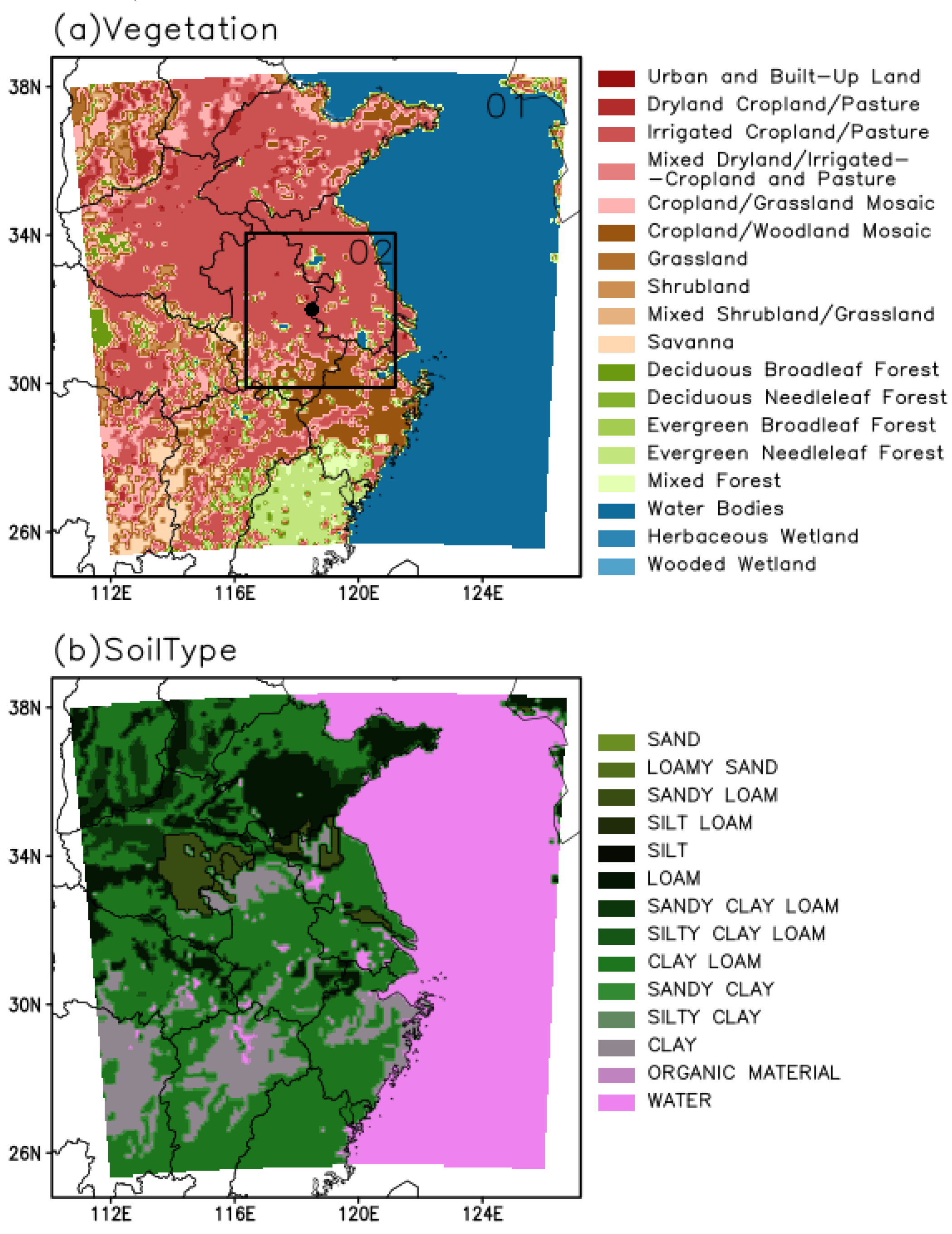
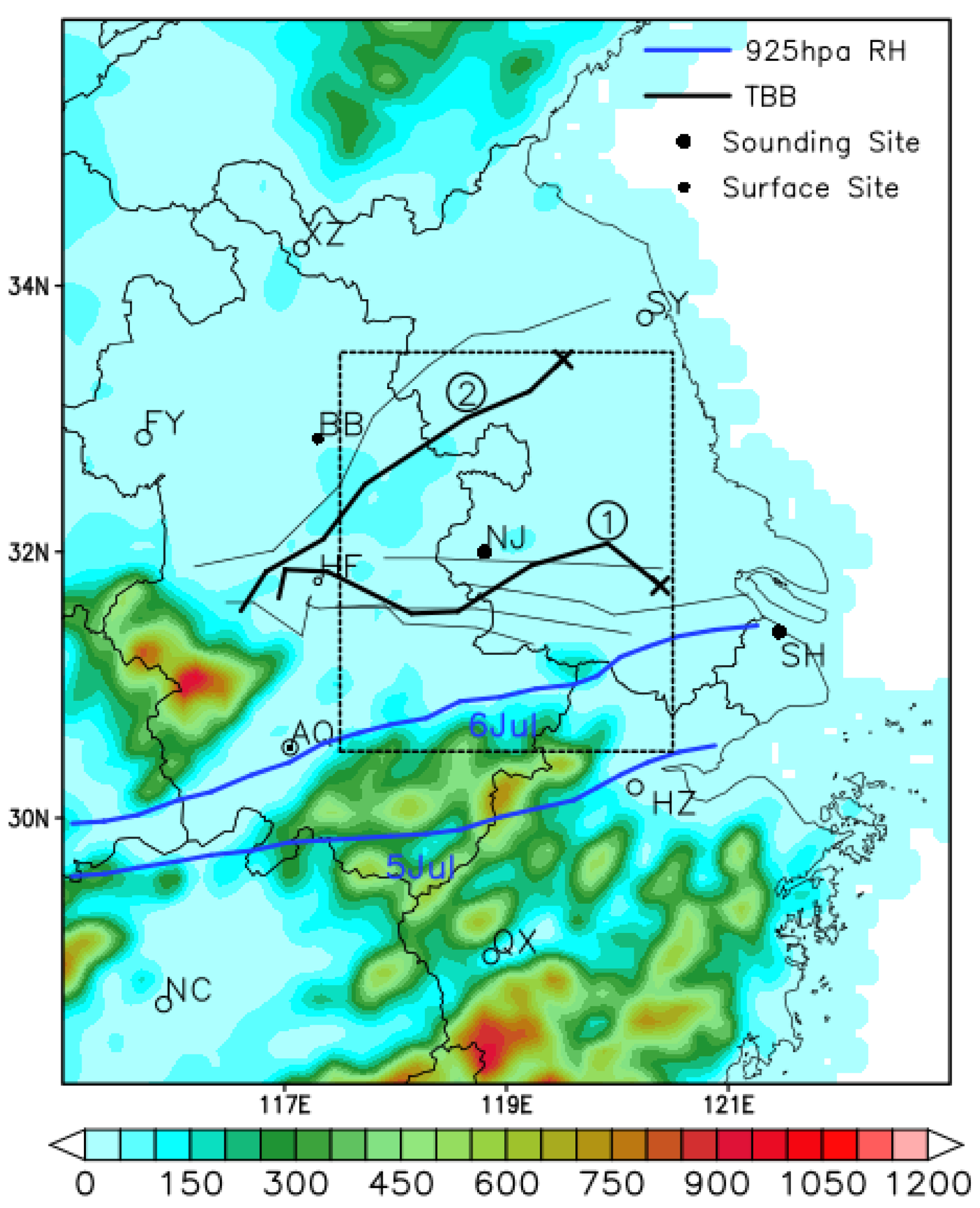
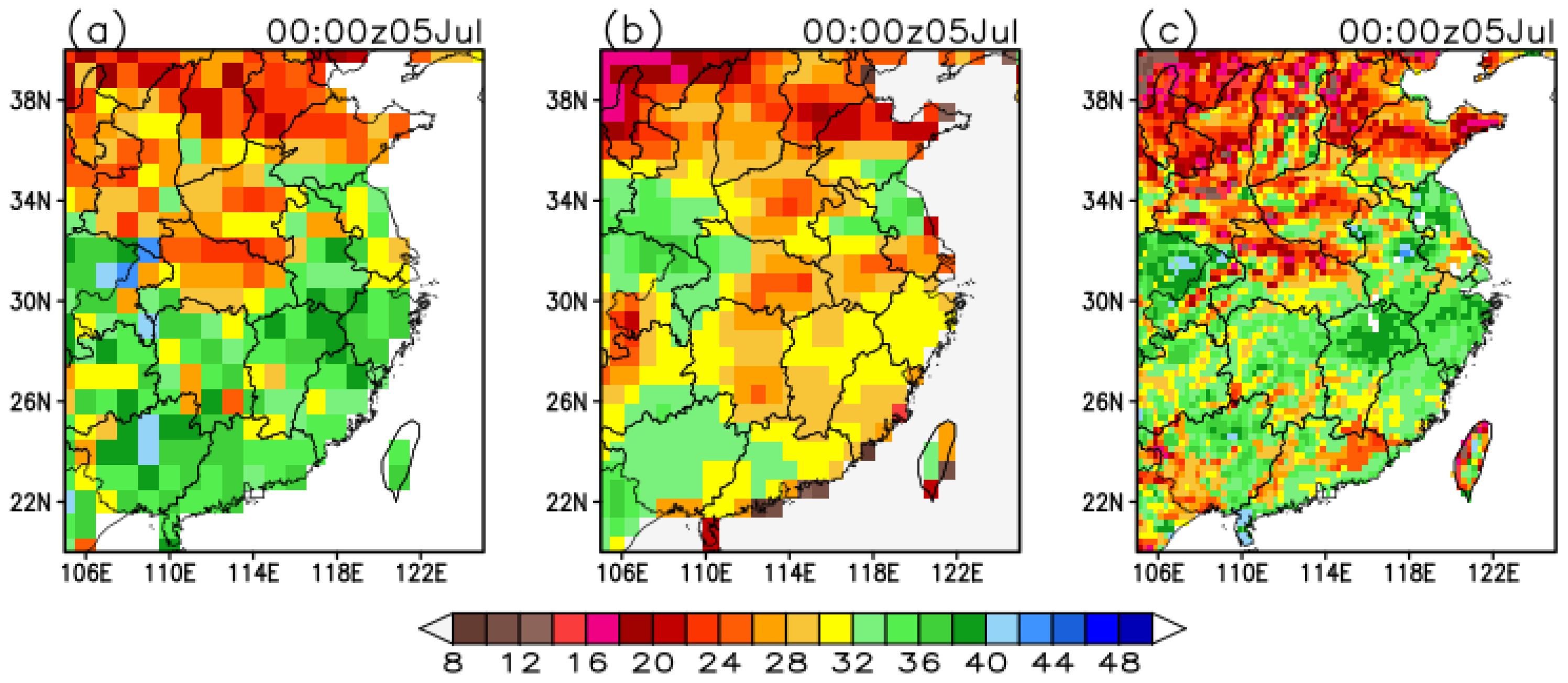
2.2. Brief Description of Frontal Rainstorm and Land Surface Conditions

The large-scale synoptic conditions that characterized July of 2013 are typical of this time of the year, with frontal rainfall systems frequently crossing the Yangtze River Basin. On the morning of 5 July, two troughs lie in the geopotential and thermal isopleths at 500 hPa while the Western Pacific Subtropical High lies to the south of China; an intense Westerly Wind Jet (WWJ) at 200 hPa parallels the north edge of our studied area and a strong Low-Level Jet (LLJ) at 850 hPa extends to the south of the Yangtze River Basin and “meets together with” the upper WWJ at the Yangtze River estuary (not shown). The synoptic conditions could favor frontal MCSs [66]. While the dry and cold air from the north joins the warm and wet air from south and acts as the so-called “Meiyu” front, it further forms clear humidity gradients near the land surface (Figure 2). From 5 July to 6 July, the front moves north and leans northeast. The gravity waves generated by the topography in the cold pool north of the front, with the cooperation of the front and large-scale favorable conditions, form into two MCSs (Figure 2).
The hourly temperature of brightness (TBB) gridded at 4 km, derived from the MTSAT-1R data provided by the Center for Environmental Remote Sensing of Chiba University of Japan (CEReS), are used as a reliable description of the frontal MCSs’ movements. On the late afternoon of 5 July, a multicellular storm (MUS) within a “cloud street” which lies in the south of the Yangtze River Basin when the coldest cap is less than −50 °C has lasted for several hours. On the late afternoon of 6 July, an isolated thunderstorm cell (TUS) lies to the north of Nanjing city, has lasted for three hours, and the coldest cap exceeds 1° × 1° (Figure 2). Surface cooling has been captured when the two convective lines cross this area (Figure 3). From 3 a.m. to 6 p.m. UTC on 6 July, the pressure of the BengBu (BB) site first increases and later decreases (Figure 3b); this indicates that a low-mesoscale high perturbation has developed with the mature TUS. On 5 July, the pressure of the AnQing (AQ) site mainly increases, indicating the mesoscale high perturbation in the MUS (Figure 3a). Although no soundings are available over the region that could experience the MUS and the TUS, a nearby thermodynamic profile of the Nanjing (NJ) site (not shown) shows a shallow and moist boundary layer with a cape of 22.33 J⋅kg−1 at 12 p.m. UTC on 5 July, while there is a deep PBL with a cape of 548.18 J⋅kg−1 at 12 p.m. UTC on 6 July.
The LLJ can bring moisture and favors low-level convergence, which can favor the nighttime (from 12 p.m. to 12 a.m. UTC) convections [66]. The winds of the NJ site show weak southwest LLJ with warm advection under 1.1 km and strong northwest cold winds above at 12 p.m. UTC on 5 July (Figure 4a), while the ShangHai (SH) site shows an opposite situation because the ocean near the SH site has highly affected the nighttime low-level winds (Figure 4c). Warm advection under 3 km and strong southwest winds, the velocity of which has exceeded 20 m⋅s−1 at 0.5 km, can be found in the NJ site at 12 p.m. UTC on 6 July (Figure 4b), and this intense southwest and warm advection also can be found in the SH site above a 0.5 km height (Figure 4d). Clearly, the LLJ has contributed greatly to the TUS on 6 July.
The main land surface characteristics in our simulations are cropland and clay loam (Figure 1b). Numerical experiments are designed by using datasets of FNL, ERA and Merged to evaluate the model simulations. Trier et al. [50] have reported that sophistication and resolution of initial soil moisture are important in a high-resolution simulation of PBL characteristics, and the soil moisture gradient can notably affect the PBL in the middle United States. Parada and Liang [67] have pointed out the spatial resolutions and data quality of soil moisture can notably affect the model outputs during a study of data assimilation. However, there are no available observations in our studied region at this specific time period. Surface soil moisture in the ERA experiment shows a positive west-to-east gradient, while both the FNL and the Merged experiments show positive south-to-north gradients, and the Merged experiment shows a sophisticated land surface (Figure 5). Zhang et al. [51] and two other later studies [68,69] suggested a spatial distribution of a climate scale that is consistent with the FNL and the Merged experiments. The Merged data shows a “climatic” soil moisture pattern, with more sophisticated soil moisture than others.

3. Model Evaluation

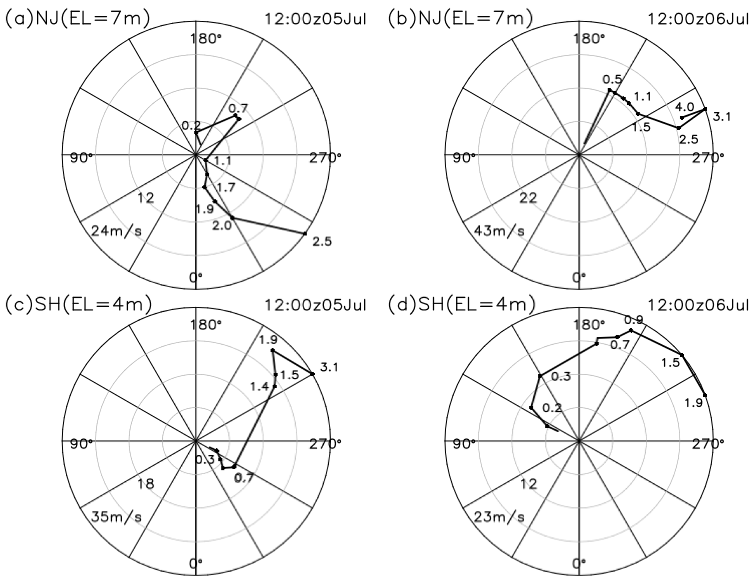
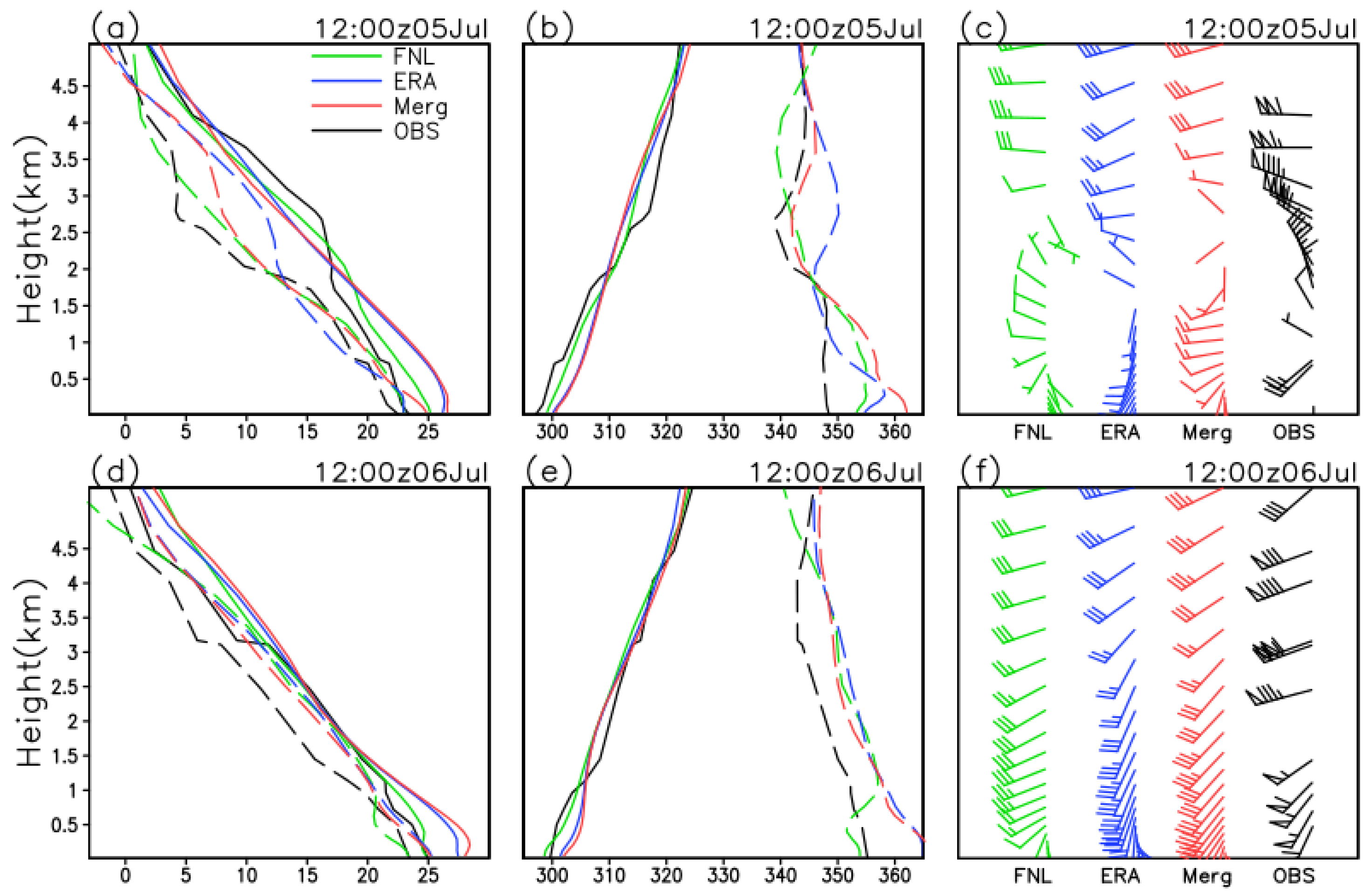
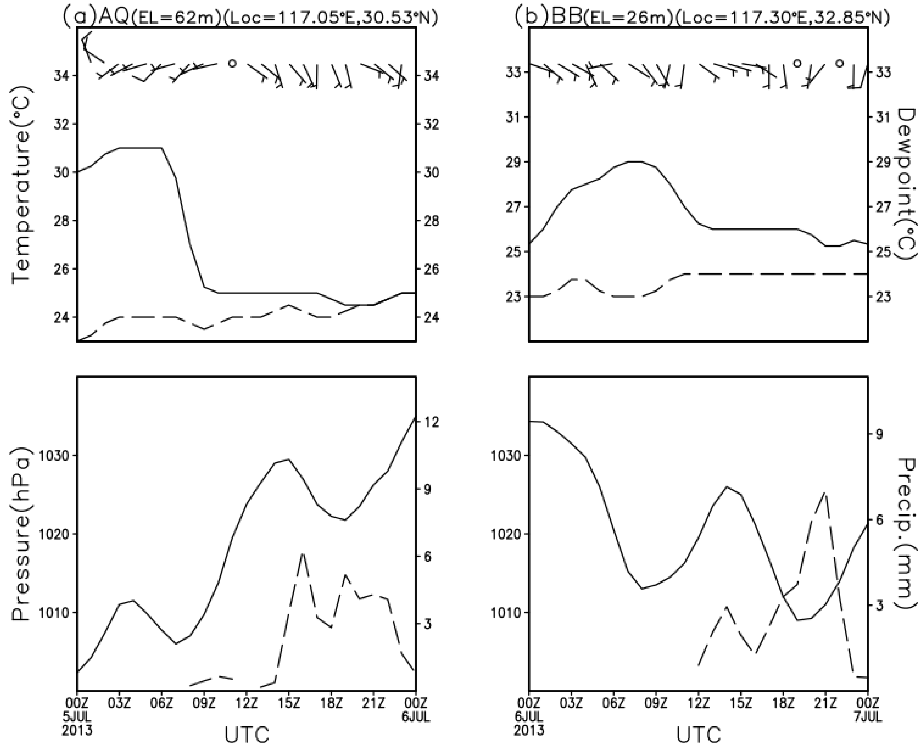
3.1. Comparison with Observation of Vertical Thermodynamic Profiles

The vertical thermodynamic profiles can represent the atmosphere conditions of a large area and they can supply the favorable or unfavorable conditions when simulating the MCS development [11]. To investigate the impact of datasets on PBL thermodynamic simulations, we have analyzed the differences between modeled and observed vertical profiles of temperature, potential temperature and winds less than 5.0 km in height at the NJ site on 5 and 6 July (Figure 6).
In the observed profiles at 12p.m. UTC on 5 July, in the lower 1.5~2.5 km a typical residual layer top can be distinguished, where temperatures are constant and inversed winds can be found. Among all the simulated profiles, the temperature (Figure 6a), potential temperature and equivalent potential temperature (Figure 6b) in this residual layer are all overestimated, indicating deep PBL, strong subsidence and moist atmosphere compared to the observation. However, in the experimental FNL the wind velocity is underestimated (Figure 6c). On 6 July, a typical residual layer top of the lower 1~1.5 km can be distinguished in the observed profiles, where temperature is constant (Figure 6d) and strongly increased potential temperature (Figure 6e) can be found. In this layer, all the simulations have overestimated the temperature and potential temperature, but have simulated the strong LLJ (Figure 6f) well. Differences between the dew point and temperature in all simulated profiles are larger than the observed profiles and this indicates an overestimation of moisture (Figure 6d).
A warmer and wetter residual layer can be found in all simulations while weaker LLJ in the FNL experiment can be found when compared to the observations on 5 July. This should be attributed to model defects and possible data differences. The warming of the potential temperature of this layer indicates intense subsidence, and the surplus moisture will favor the sustained precipitation. Generally, the experimental FNL has simulated quite different wind profiles from the observations, while the other two in ERA and Merged agree well with the observed wind profiles. Thus, this could account for differences in datasets.

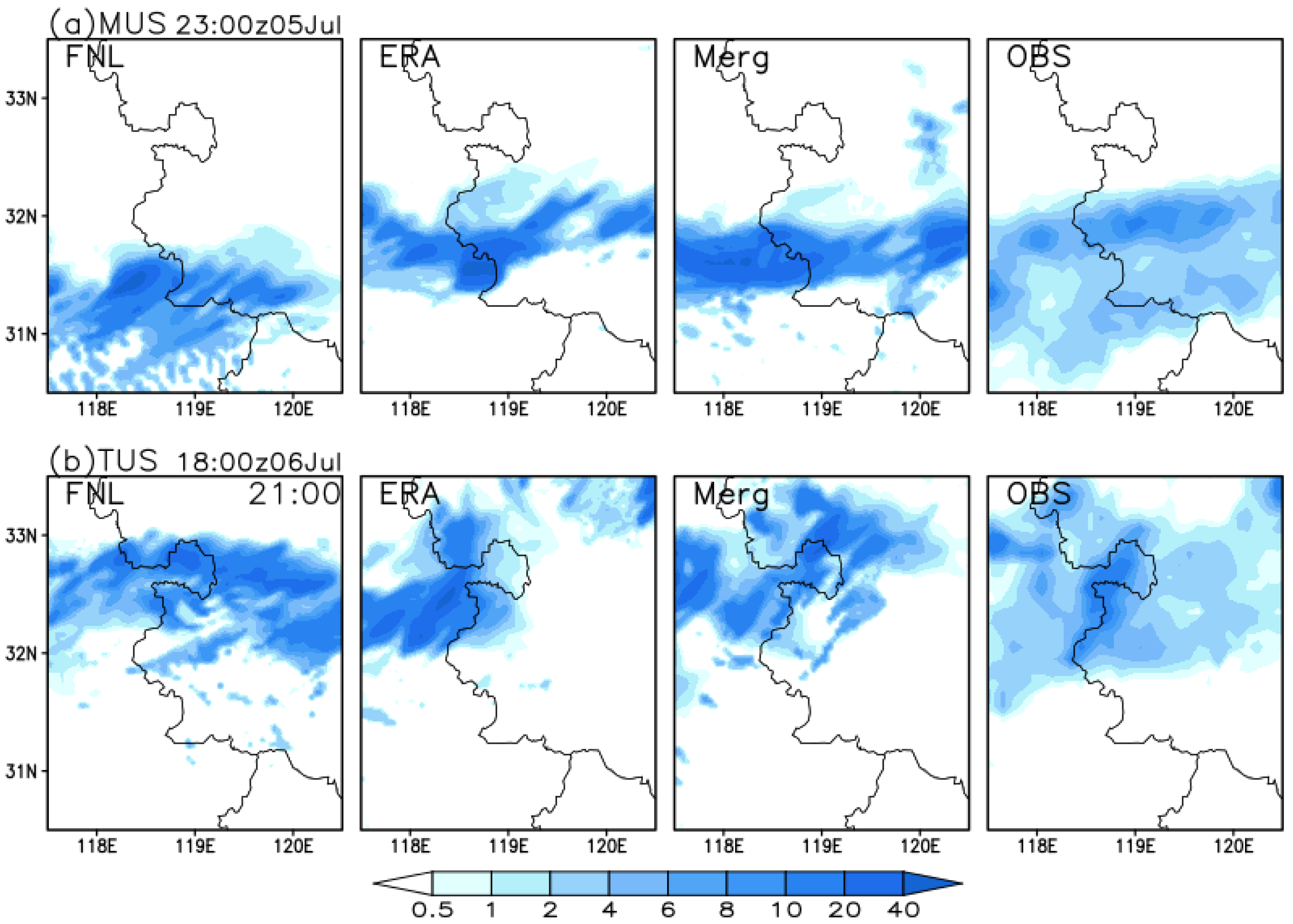
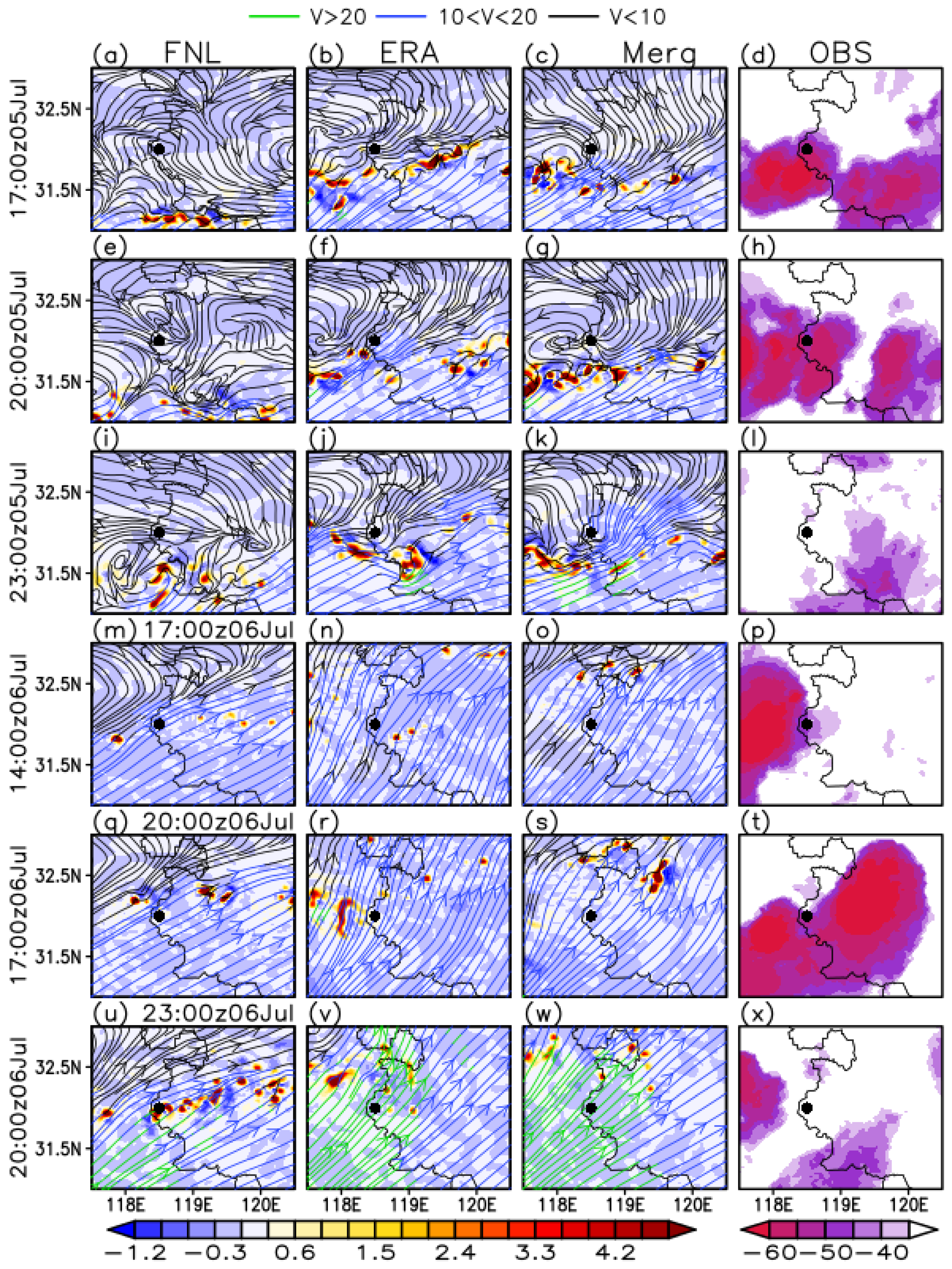
3.2. Comparison of MCSs’ Patterns and Intensity with the Observed TBB and Precipitation

Dirk et al. [11] suggested that land surface can affect MCS by verifying the low-level flow patterns and upper layer convections in West Africa. As in the Yangtze River Basin, local intensely developing convections can break the geostrophy constraint of the troposphere in small regions [70]; thus we think this method, as Dirk suggested, is valid in middle-latitude atmosphere. Firstly, the flows at the 1.5-km height and vertical velocity at the 5.5-km height, which represent the low-level convergence and the upper intense convection, are used as the MCSs’ pattern and location, respectively. The above-mentioned TBB data supplies the observed distributions of upper convections. Second, the maximum of precipitation that exceeds 50 mm⋅h−1 and the area of which exceeds 100 × 100 km2 is defined as the MCSs’ intensity by regarding the hourly Climate Prediction Center Morphing Technique (CMORPH) observations gridded at around10 km which are derived from the Chinese Meteorological Administration (CMA). Then the MCSs’ patterns and intensity are compared between the simulations and observations.
Seen from the streamlines (Figure 7), a convergence zone can be located where the inflows have turned into outflows. First, at 8 p.m. UTC on 5 July, the main pattern of MCSs shows that the MUS lies along latitude 31.5°N with several scattered cloud clusters, and this agrees well with strongest convections in the experiments for ERA and Merged; in the FNL experiment, however, the area of this convergence zone is overestimated by around 5000 km2 while the intense convections show a modification of 50 km south to observations (Figure 7e–h). Subsequently, the TUS occurs in the north of the NJ site at 5 p.m. UTC on 6 July, and the coldest cap has centered at 33°N, 119.5°E. An isolated convection of 5.5 km in the Merged experiment shows a matched location of the observed TUS and intense southwest flows where the velocity exceeds 20 m⋅s−1; the FNL experiment, however, shows weak LLJs and a northward modification at 8 p.m. UTC on 6 July, while the ERA experiment shows a westward modification (Figure 7g–t). Between the model experiments of FNL, ERA and Merged, quite different low-level flow patterns of two main MCSs are found, when both of the modeled MUS and TUS in the FNL experiment occur at slightly different times. Clearly, both the ERA and Merged simulations have reproduced more suitable cyclonic patterns and smaller modifications of convections than FNL.
A line-like belt of precipitation of MUS is reproduced in all experiments at 11 p.m. UTC on 5 July; however, a modification of this belt by around 50 km south of the observation can be found in the FNL experiment, while the ERA experiment has underestimated the strongest precipitation (Figure 8a; ERA). Both the ERA and Merged experiments show a clearly south-to-north rain belt of TUS at 6 p.m. UTC on 6 July, which fits the observation well; however, the FNL experiment has missed this pattern and the ERA experiment shows a slightly westward modification (Figure 8b). The strength of MCSs is overestimated in all experiments, while the rain belts of the Merged experiment agree better with the observations than the others.
Earlier, it was mentioned that differences of datasets can cause wind differences and possible moisture differences in the residual layer, which should account for the differences in MUS and TUS among the three simulations. That the FNL experiment has simulated weak LLJ on 12 p.m. UTC 5 July possibly causes a southward modification of the convergence line of MUS later. Additionally, a moister and warmer atmosphere in all simulations could result in stronger convections in contrast to the observations.

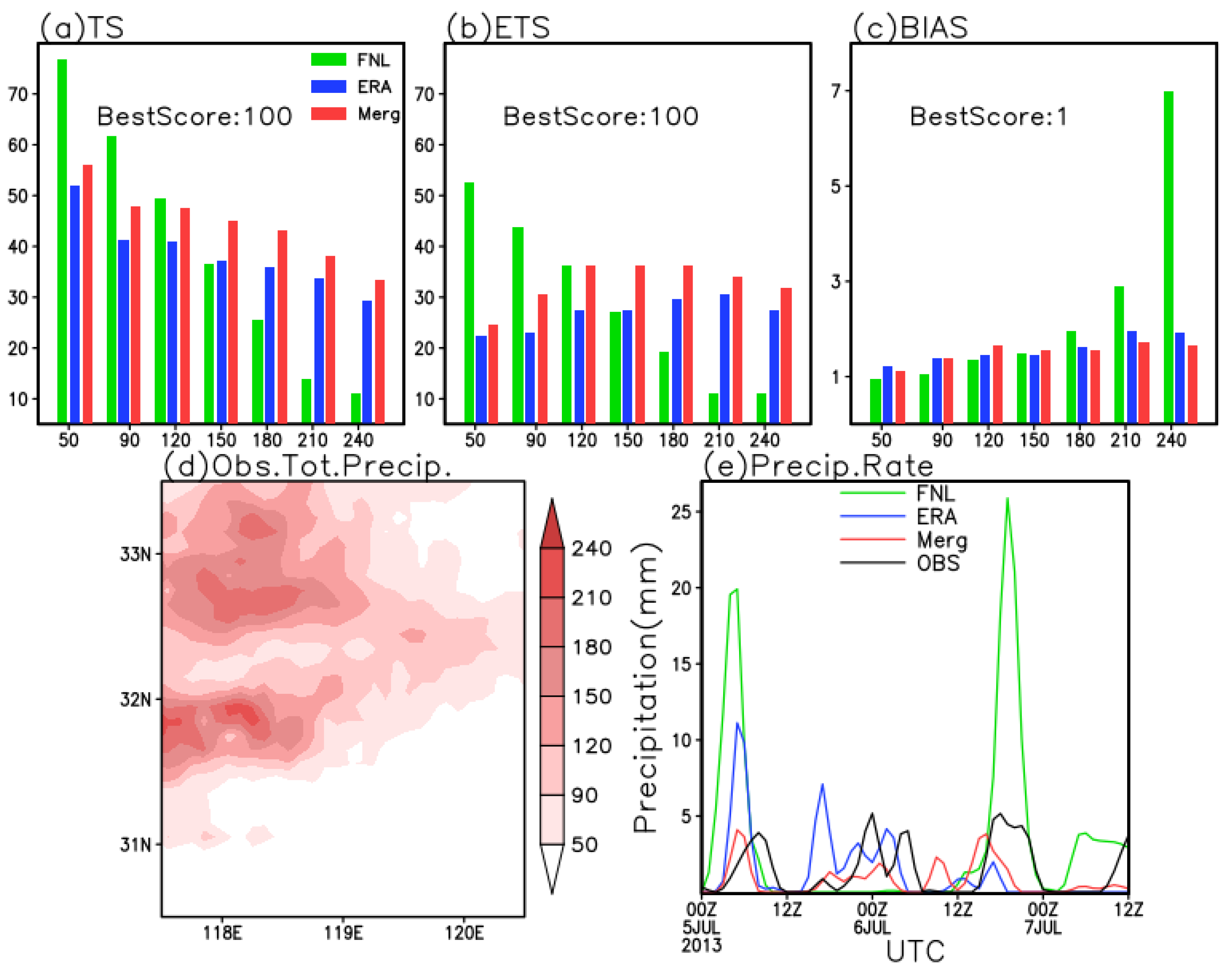
3.3. Comparison of Total Precipitation and Precipitation Rate with Observation

Several widely used skill scores are used as a quantitative evolution of total precipitation during the 2.5-day simulations, and precipitation rates are compared with the CMORPH products. In the observed total precipitation, two rain belts along the two ongoing discussed convergence lines agree well with the MCSs’ patterns (Figure 9d). However, in the FNL experiment a southward modification of the rain belt is found and the total precipitation in the north district is clearly underestimated (not shown), which is consistent with previous results.
For a certain referenced area, at any given precipitation threshold over an accumulation period, the observed rain area exceeding the criterion is O and the model-predicted area is F. Their intersection (e.g., the hit area) is denoted by H, while the entire verification domain is N. The above skill scores are defined as (more detail described by Wang [71]):
TS = 100 × H / ( O + F H ) ,
ETS = 100 × ( H R ) / ( O + F H R ) ,
R = ( O / N ) × ( F / N ) × N = F × ( O / N ) = O × ( F / N ) ,  and
BIAS = F / O
Thus, the TS has a value between 0 and 100 (as the hit area cannot be greater than the union of O and F), and a higher (lower) value represents better (poorer) performance. Due to this assumption of R being random and thus reflecting no model skill, it is excluded from the calculation of equivalent threat score (ETS) and is therefore subtracted. As the same TS or ETS can result from either an over-forecast or an under-forecast of rain by the model, thus the BIAS often needs to be provided to interpret the verification results more accurately.
In 50~120 mm thresholds, the TS (Figure 9a) and ETS (Figure 9b) in the FNL experiment are higher than the other two simulations, but lower for heavier thresholds; the BIAS scores of FNL experiments are higher than that of the other two in 180~240 mm thresholds, but lower for lighter thresholds (Figure 9c). Both the Merged and the ERA simulations reproduce more accurate precipitation than the FNL experiment for heavier thresholds. The Merged experiment shows less biases of precipitation rate than the other two experiments when compared to the observations (Figure 9e).
Seen from Table 2, the Merged experiment has general improvements for both TS, ETS and BIAS. The Merged experiment reproduces a slightly lower BIAS than ERA for most thresholds except 120 and 150 mm, as the lower BIAS indicates being closer to the Best Score (Figure 8). Especially, the TS and ETS increased by 6.61% and 7.74% for the 90-mm threshold, respectively.
In general, the FNL experiment has reproduced a larger deviation in PBL profiles, MCSs and precipitation compared to the observations than ERA and Merged. However, Merged reproduces MCSs more consistent with the observations and better statistical results in precipitation than ERA. The major differences of the three experiments are the above-mentioned varying datasets (as FNL and ERA) and soil moisture (as ERA and Merged). This indicates the necessary use of both ERA-Interim reanalysis and Global Land Data Assimilation System (GLDAS) soil moisture in improving model results for both weather forecast and agricultural irrigation. Therefore, to some extent, sophistication in soil moisture can notably impact the model performance of frontal systems.

4. Sensitivity of the Rainstorm to Soil Moisture

We use the Merged run as the control experiment (CTL) and sensitivity experiments are conducted as two ensembles of systemically increasing (decreasing) initial soil moisture (as summarized in Table 1), which are defined as WP (DP) ensembles. The near-surface PBL characteristics and precipitation are compared between the CTL and sensitivity experiments.
In order to investigate the possible responses of this modeled rainstorm to soil moisture, we use the averaged differences between the dry or wet ensembles and the CTL experiment to assess the determined “DRY” and “WET” biases. We define 1 N k = 1 k = N X d k and 1 N k = 1 k = N X w k as the mean “DRY” and “WET” statements, and D R Y =   1 N k = 1 k = N ( X d k X c t l ) and W E T =   1 N k = 1 k = N ( X w k X c t l ) as the “DRY” and “WET” biases, in which X is the averaged state variable of our studied area at a given height, k   is the ensemble member and N is the number of members ( N = 3 ). X d k ,   X w k and X c t l mean the variable X in DP, WP and CTL experiments. This will help us understand the relations in case of some unrealistic factors (for instance, the initial soil moisture in the WP15 experiment somehow possibly exceeds the field capacity, and this may cause fake responses of atmosphere at the beginning). The possible relations between the surface fluxes, PBL thermodynamic variables and precipitation are distinguished by comparing the variations of ongoing discussed biases in PBL to the mean statements of near-surface variables and also comparing the variation of these biases in PBL to the variation of biases in precipitation over dry or wet surfaces.

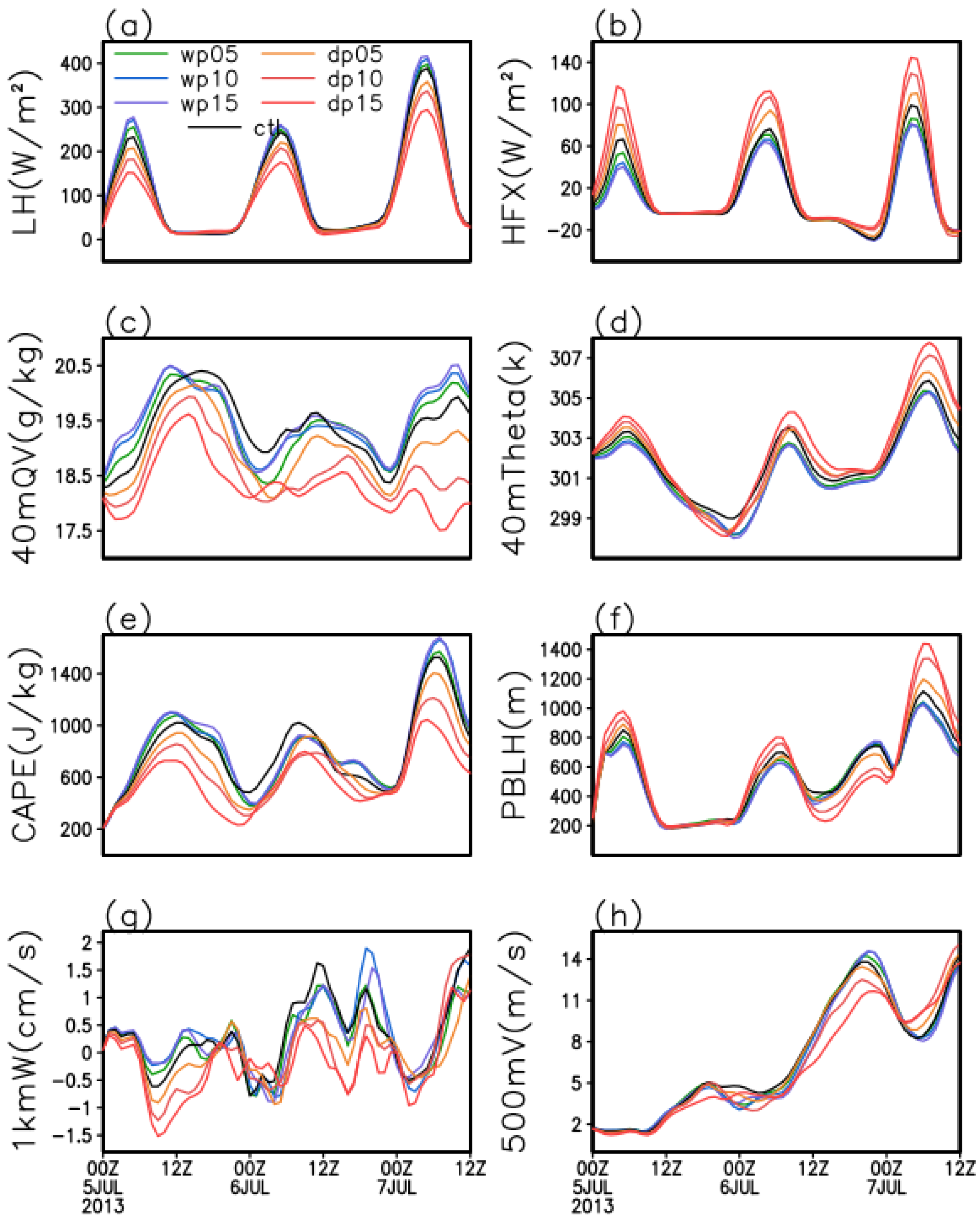
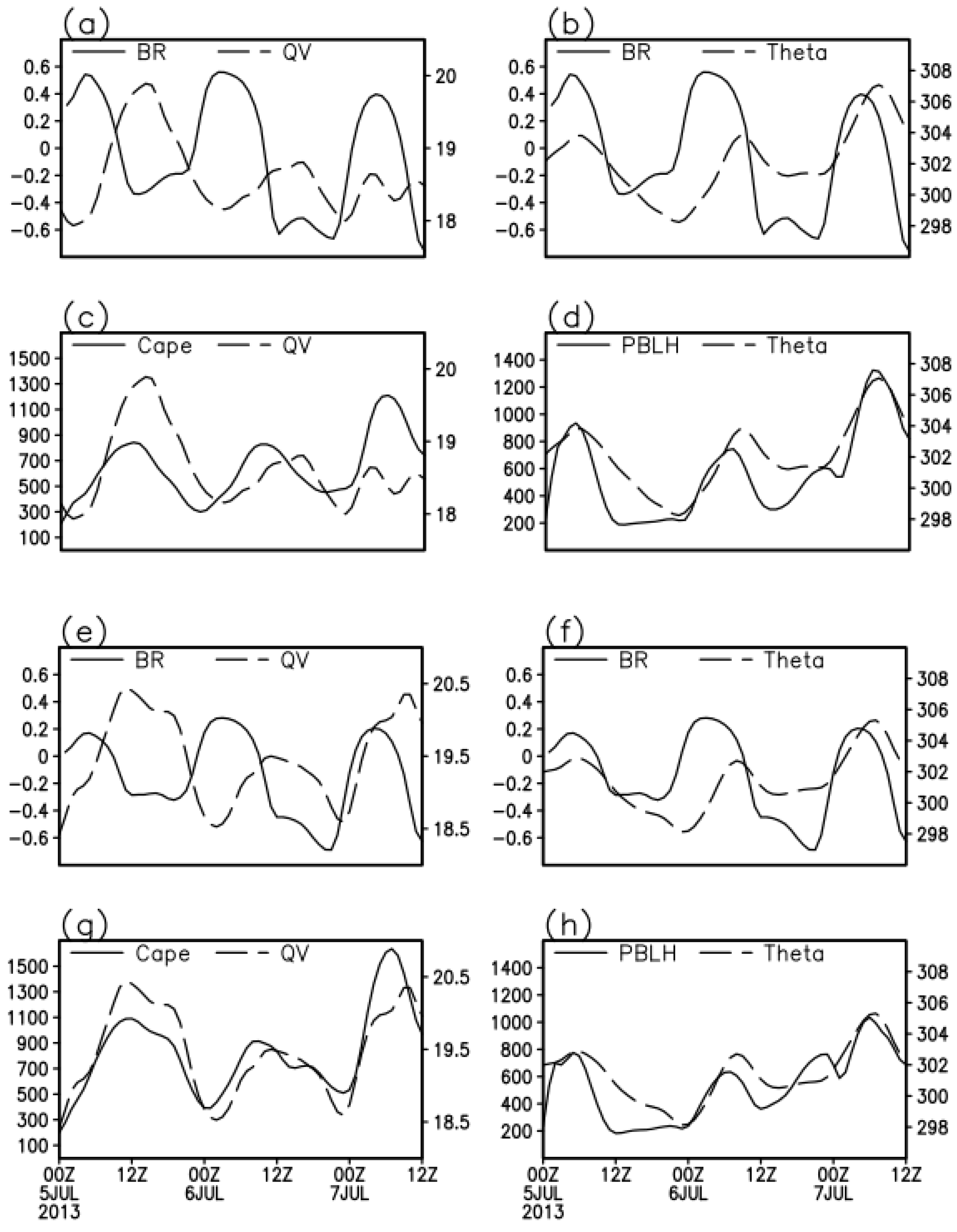
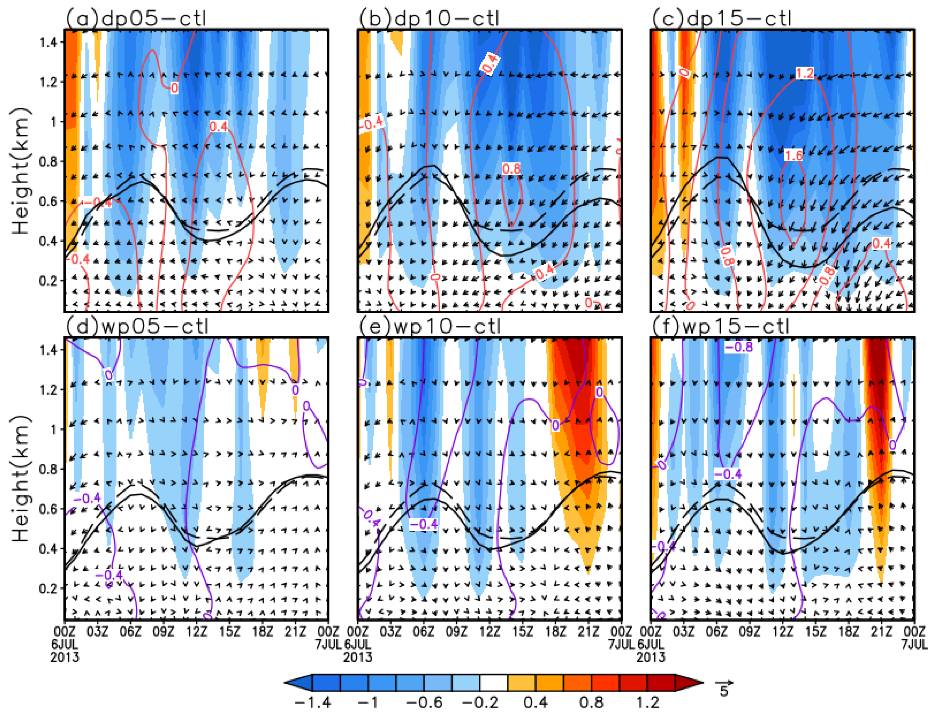
4.1. Sensitivity of Near-Surface and Upper PBL Characteristics to Soil Moisture

The diurnal variations of near-surface thermodynamic variables are examined by comparing the sensitivity and the CTL experiments. The largest differences in 40-m potential temperature (Theta) are found between the DP15 and the CTL experiments, where a maximum bias about 2.5 K is found at 5 a.m. UTC on 7 July (Figure 10d). However, the largest differences in the 40-m water vapor mix ratio (QV) are found between the DP10 and the CTL experiments, with a maximum bias of 4 g⋅kg−1 at 6 a.m. UTC on 7 July (Figure 10c). These near-surface moisture and temperature variables show consistent variations with surface fluxes, and this indicates the soil moisture has modulated the near-surface thermodynamic conditions during this event. Moreover, DP ensembles show relatively larger differences in near-surface variables than the WP ensembles when compared to the CTL experiment. Recall that the top-layer soil moisture of our study area in the Merged run mostly exceeds 30% (Figure 5), where the dominant field capacity is about 40%, indicating that the soil moisture availability fields of wet ensembles (as WP10 and WP15) are mostly saturated with intense moisture stress, which could account for the larger differences of both the latent heat fluxes (LH) (Figure 10a) and sensible heat fluxes (HFX) (Figure 10b) in the DP ensembles compared to the CTL versus the WP. Thus, due to the very wet initial soil conditions, the near-surface thermodynamic variables are more sensitive to the dry surface, and these results are consistent with the previous results in climatic scales [43,46].
The convective available energy (CAPE) for the most unstable 500-m-deep air parcel and the PBL height (PBLH) are also examined. The differences of PBLH among all simulations mostly show positive biases in the DP experiments compared to the CTL experiment (Figure 10f), and the differences of CAPE (Figure 10e) show negative biases; however, negative biases of PBLH are found between 12 p.m. UTC on 6 July and 12 a.m. UTC on 7 July when the TUS occurs. Furthermore, in the 1-km vertical velocity (W) referenced as the vertical mixing of daytime at the PBL top, negative biases are found in DP experiments compared to the CTL experiment (Figure 10g). At the time when the TUS occurs, the largest difference (~6 m⋅s−1) of 500-m meridional wind velocity (V) referenced as the dominant movement of low-level atmosphere is found in the DP15 experiment compared to the CTL experiment (Figure 10h). The variations of the PBLH and V differences on 6 July indicate that atmospheric conditions notably influenced the PBL winds during the nighttime when the surface fluxes decrease.
The relationships between surfaces fluxes, near-surface variables, CAPE and PBLH are identified by the variations in “DRY” and “WET” statements (Figure 11), in which the Bowen Ration (BR) is defined as HFX/LH, representing the dominant surface fluxes. The BR increase shows consistent variation with the near-surface temperature increase (Figure 11a,e) and the near-surface moisture decrease (Figure 11b,f). This implies the near-surface variables are significantly modulated by the surface fluxes. The CAPE variations accompanied the near-surface moisture (Figure 11c,g) and the PBLH variations similarly with the near-surface temperature (Figure 11d,h). In fact, the differences of latent heat flux in the low-level atmosphere, induced by differences in near-surface moisture, can cause moist static energy (MSE) differences (not shown) during the late afternoon when the largest differences in CAPE can be found in both “DRY” and “WET” statements. The differences of CAPE between the CTL and sensitivity ensembles resulting from latent heat can be affected by near-surface moisture here, while the differences of PBLH during the daytime are mostly attributed to the differences of surface temperature.
In general, the local heating and moistening mainly dominate the diurnal characteristics of the near-surface thermodynamic characteristics and are likely affected by the atmospheric forcing. Results show a positive feedback between the soil moisture and the PBL, which means wetter soils favor higher latent heat flux, lower sensible heat flux and shallower PBL height; net fluxes at the wetter surface thereby increase the moist entropy flux into the PBL, which strengthens the MSE (increase the CAPE) in the PBL and decreases the PBLH. These act in concert to increase the potential for convective activities, while the drier surfaces act in an opposite way. The relations between soil moisture and the PBL are consistent with many previous works of greater scales [7,72]. However, negative anomalies of 500-m meridional winds and PBLH in DP ensembles on 6 July indicate that atmospheric controls have played an important role in the relationships between soil moisture and the PBL when the surface impact weakens.

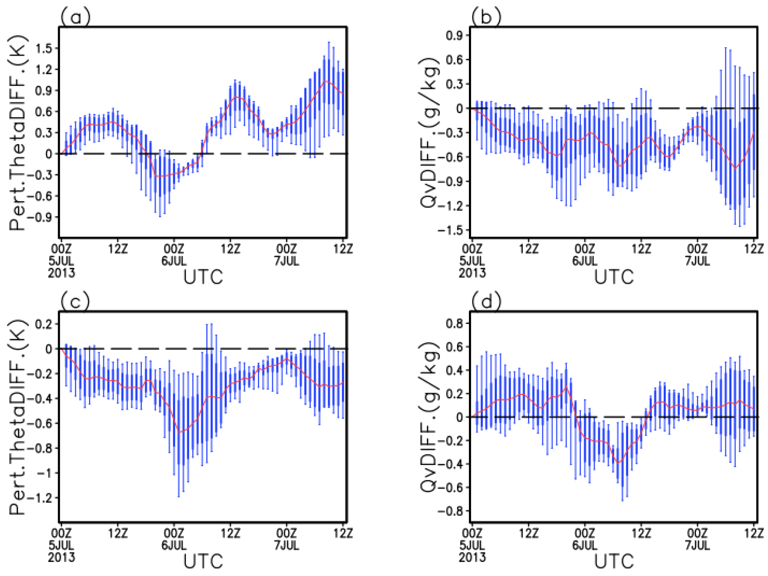
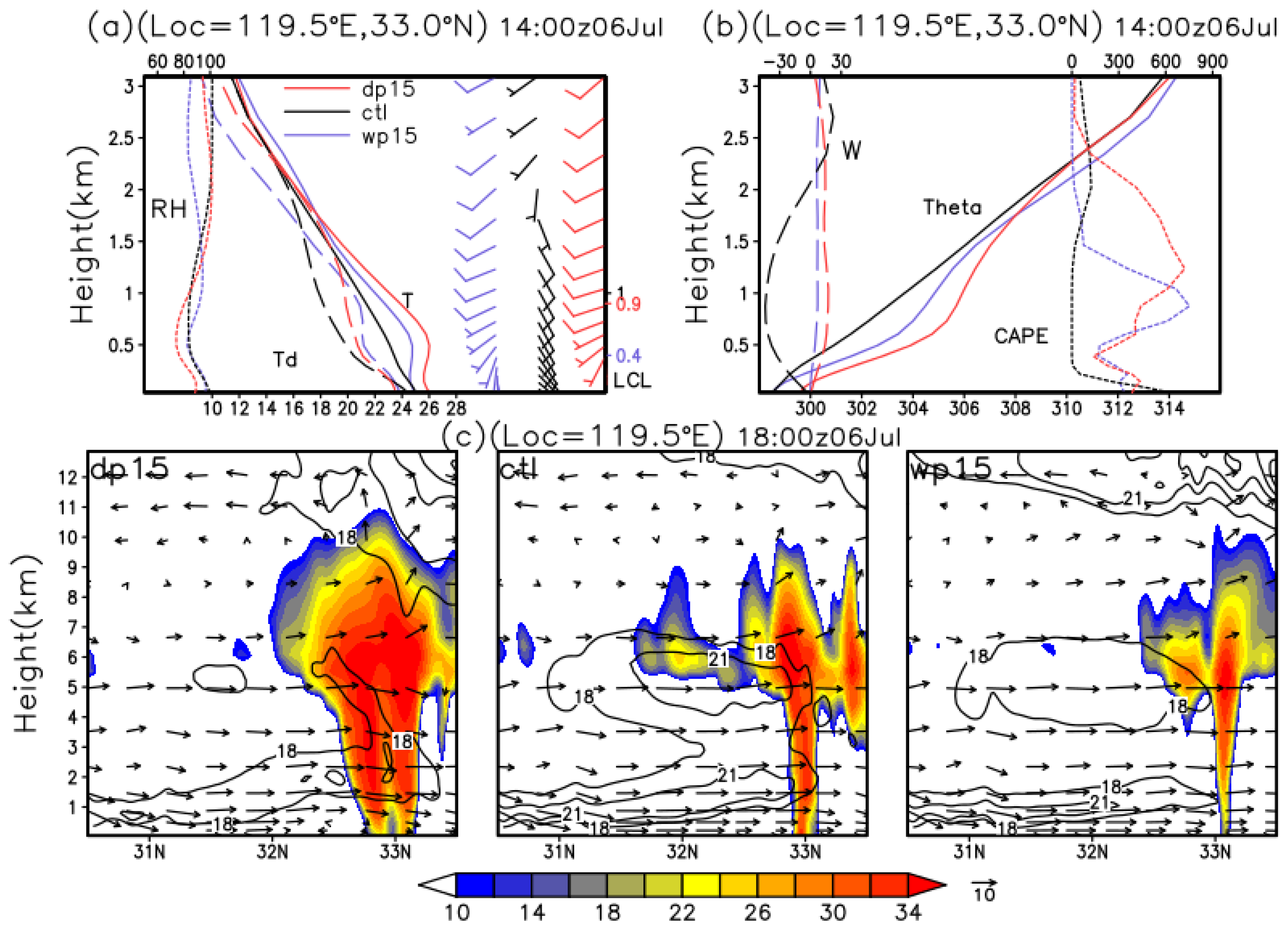
4.2. The Possible Relations between Land Surface and Upper MCSs

The ongoing discussed soil moisture–PBL relationships have established the knowledge of interactions that are regulated through releasing the MSE during the late afternoon over wet soil and strengthening the daytime turbulence mixing over dry soil, also highlighting the significant influences of atmospheric forcing on these relations. We have examined the characteristics of the “DRY” and “WET” biases of moisture and temperature in PBL, which is different from the Findell’s method [20], to identify the impact of atmospheric controls on the PBL. Also, the reasons for the largest differences of low-level winds and negative anomalies of PBLH in the TUS period are examined.
Here the mean “DRY” and “WET” biases represent the determined differences of the PBL between the DP, WP ensembles and the CTL experiment at 0~1.5 km height, and the deviations and standard deviations show the variations of these biases in the vertical layer (Figure 12). If we assume the PBL conditions are mostly affected by the surface fluxes, then temperature in mean “DRY” biases and moisture in mean “WET” biases should be positive, which means above the ZERO line (where the biases are equal to 0); however, negative biases could be found on 6 July, which means the atmospheric controls of a “cold invading” in the PBL are significant (Figure 12a). During this period the moisture in “DRY” biases (Figure 12b) and the temperature in “WET” biases (Figure 12c)are more likely affected by the surface fluxes. The error bars show the chaotic variations of these biases in the PBL. These negative “DRY” biases in temperature mean the cooling of the PBL over dry surfaces, while the negative “WET” biases in moisture indicate a “dry invading” in the PBL (Figure 12d). The reasons causing this “cold invading” over dry surfaces and “dry invading” over wet surfaces are complicated because the large-scale soil-PBL interactions can affect the convective-scale relations, which will not be discussed in this paper.
The PBLH differences, 0~1.5 km vertical velocity differences and horizontal wind vector differences between sensitivity and the CTL experiments are further present to examine the PBL variable differences that might be affected by the cold or dry invading (Figure 13). Firstly, the negative potential temperature differences in the DP experiments (QV differences in WP ensembles) can be observed in the whole PBL during the daytime (before 12 p.m. UTC) when the PBLH increase (decrease) indicating the cold (dry) invading occurs. Moreover, the horizontal wind vector differences in the DP (WP) experiments rotate anti-clockwise (slightly rotate clockwise) at around 12 p.m. UTC when the PBLH decreases (increases), during which time these differences in the DP experiments are almost three times of that in the WP experiments. In addition, vertical wind differences in the WP ensembles are negative and turned positive at around 6 p.m. UTC, with the maximum of 2.5 m⋅s−1 in the WP15 experiment (Figure 13c); in DP ensembles these differences are mostly negative. Generally, these descending biases during the daytime indicate the inhibition of vertical mixing resulting from the stronger invasion of cold air in both the DP and WP experiments as compared to the CTL, while the PBLH increase in DP ensembles indicates the impact of near-surface warming. Also, these intense descending motions during the nighttime in DP experiments indicate larger wind divergence in the PBL, which can cause weakened LLJs (Figure 10h) and decreased PBLHs ([63]; Figure 10f), and further suppress low-level convections while the WP ensembles show an opposite trend during the nighttime.
The large-scale forcing of atmosphere can affect the PBL in various ways besides the surface fluxes, for example the remote moisture transpiration and temperature advection through environmental winds. We mainly discuss how the daytime surface fluxes affect the PBL under these environmental forcing conditions (e.g., the warm front and the upper vertical shear). Recall the fact that, in the DP15 experiment, weak moistening and intense warming can be distinguished from the near-surface thermodynamic variations, accompanied by weakened LLJs during the late afternoon on 6 July (Figure 10); this indicates that a larger divergence of TUS in the DP15 experiment is simulated compared to other experiments. The largest anomalies of 500-m V in the DP ensembles can result from daytime PBL differences, and an explanation is provided for these differences. First, we relate the differences of nighttime low-level winds to the different TUSs. Subsequently, we link the different TUSs to the differences of PBL potential temperature and moisture, which are likely affected by surface fluxes and atmosphere conditions.
The DP15 experiment has generated a strong TUS at 6 p.m. UTC on 6 July (Figure 14c), accompanied by a weakened southward LLJ, which should be attributed to the northward flows induced by the low-level divergence of a mature thunderstorm. The thermodynamic profiles of 2 p.m. UTC have showed a quite lower CAPE in the WP15 and DP15 experiments than the CTL experiment (Figure 14b). As for the “cold invading” in DP ensembles in the daytime of 6 July (Figure 12a), the decreased potential temperature of PBL in both the WP15 and DP15 as compared to the CTL experiments can be found (Figure 14b), and this could favor the development of ascending motions caused by the thermal perturbing of the PBL top and further assemble more CAPE in both the WP15 and DP15 experiments. However, the “dry invading” in WP ensembles favors the unsaturated conditions at the top PBL (Figure 14a), and causes quite a lower lifting condensation level (LCL) in WP15 than in the other two experiments, which is inconvenient for strong systems (Figure 14c). In addition, the weak winds of the WP15 and DP15 experiments could favor the development of MCSs at an early stage (Figure 14a). Many previous studies have suggested the environmental winds have modulated the ways of the soil-moisture-PBL relationships at convective scales [11,34,35]. However, the PBL wind differences indirectly resulting from the land surface characteristics through the MCSs are different from the 24-hour studies [38,40].

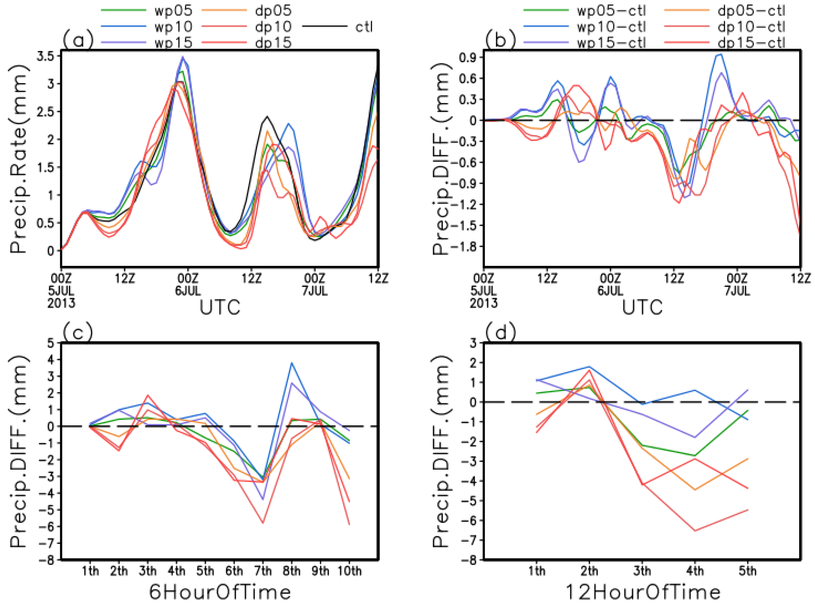
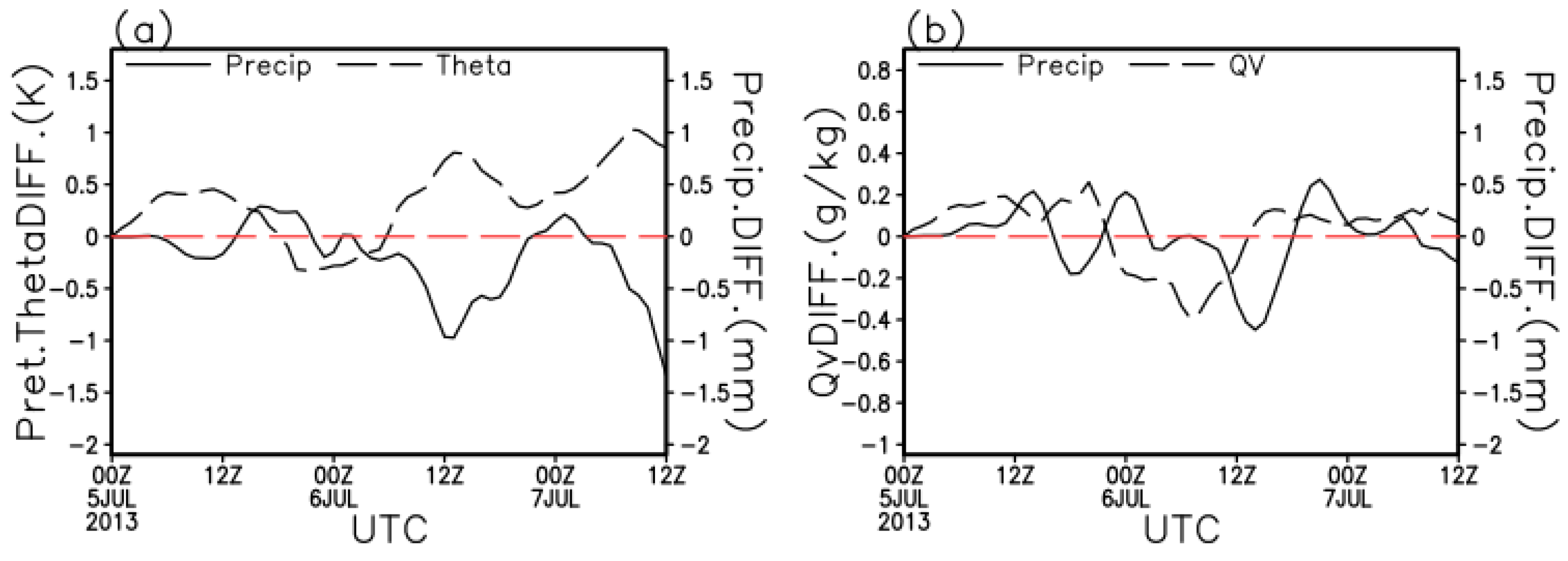
4.3. Sensitivity of Precipitation to Soil Moisture

The two peaks of the precipitation rate in all experiments show comparable relations with the two main MCSs of this 2.5-day rainstorm; in the WP ensembles, a 2-h backward modification of these peaks in the TUS period indicates that, in the WP ensembles, the TUSs have occurred almost two hours later than that in both the DP and CTL experiments (Figure 15a). In addition, in the DP experiments, differences in the precipitation rate are small and mostly negative compared to the CTL experiment except for small positive biases at around 3 p.m. UTC on 5 July or at 12 a.m. UTC on 7 July. In the WP experiments, small and positive biases can be found over most time periods, during which the maximum is ~0.5 mm at 12 a.m. TUC on 6 July; however, small and negative biases are reproduced between 3 p.m. and 6 p.m. UTC on 5 July (Figure 15b). Clearly, the DP ensembles have reproduced smaller precipitation rates than the CTL experiment, while the WP experiments have reproduced larger precipitation rates. The precipitation rates in DP and WP show consistent variations. These positive (or negative) biases in WP (or DP) ensembles are relatively smaller than 1 mm and seem to vary in different time periods.
We have further examined differences of the 6-h and 12-h total precipitation between the DP, WP and CTL experiments. In the DP ensembles, the differences of 6-h (Figure 15c) and 12-h (Figure 15d) precipitation compared to the CTL experiment appear to be negative in most time periods except the beginning time, which indicates that less precipitation has been reproduced in DP ensembles by the MUS; in the WP ensembles these differences show small and positive values at beginning but they become negative in the TUS period. Larger precipitation differences in the DP ensembles than in the WP ensembles indicate that precipitation is more sensitive to dry surfaces than wet. Additionally, decreased precipitation can be found in both the DP and WP ensembles, which are mostly affected by the different MCSs induced by different PBL conditions as has been discussed.
The comparative relations between precipitation and the PBL thermodynamic conditions are identified by the variations of precipitation differences and the mean PBL temperature (moisture) differences in the “DRY” and “WET” biases (Figure 16). Precipitation increase varies consistently with the temperature decrease over dry surfaces and the moisture increase over wet. Temperature increase over dry soil deepens the PBL and further suppresses the MSE from releasing in the PBL, and then it weakens the low-level convections; moisture decrease shows the opposite effect. This relation is more significant in “DRY” biases than in “WET” biases, indicating the effect of the initial wet surface. However, the atmospheric control (defined as the negative biases in temperature over dry surfaces or moisture over wet surfaces in Section 4.2) has greatly contributed to negative biases in precipitation over both wet and dry surfaces.
The relationships between land surface and PBL in this modeled rainstorm are well established in Section 4.1, and the indirect relations between PBL and low-level winds modulated by nighttime MCSs have been analyzed in Section 4.2. Regarding the soil moisture-precipitation feedback [9], the net surface fluxes increase (decrease) over wet (dry) soil, further increase (decrease) the MSE in the PBL and decrease (increase) the PBL depth, thus increasing (decrease) the potential convective activities and precipitation. Additionally, the sensitivity of precipitation in many previous works has been studied by using various measurements, such as maximum precipitation [19], peak precipitation [10] and precipitation frequency [34]; trends of positive feedbacks between soil moisture and precipitation are suggested in their studies, though these feedbacks can be affected by surface variability, environmental factors and model parameterization. However, in this study, decreased precipitation can be found over both wet and dry soils (Figure 14b). The significant wind anomalies induced by the nighttime TUS differences which can be affected by both the late afternoon surface and atmosphere conditions have played a dominant role in suppressing the low-level convections during nighttime when surface impact weakens, and the atmospheric controls during daytime show a clear relationship with precipitation decrease. This indicates that frontal forcing has suppressed the above-mentioned feedbacks during this event.

5. Conclusions and Discussion

A typical 2.5-day rainstorm in the Yangtze River Basin during the East Asia summer monsoon, including a multicellular storm (MUS) and a subsequent thunder storm (TUS), is studied by using the WRF model (ARW, Version 3) coupled with the Noah LSM model and different reanalysis (as FNL, ERA and Merged; see Section 2), in order to evaluate the model results by comparing the PBL, MCSs and precipitation in the simulations compared to the observed rainstorms. Results show that MCSs are reproduced in all simulations with different PBL profiles, low-level stream patterns and precipitation, showing that (1) both the ERA and Merged experiments agree better with the observations than the FNL experiment; (2) fewer biases of MCSs and precipitation are reproduced in the Merged experiment than in the other two experiments. These differences, resulting from different sophistications of atmospheric conditions (as FNL and ERA) and soil moisture (as ERA and Merged), indicate that soil moisture has significantly influenced the patterns of MCSs and precipitation in the convective-scale simulations.
The Merged simulation is the best duplicate of this observed rainstorm among all the above experiments, and six following sensitivity experiments with systematically increased and decreased soil moisture (WP and DP ensembles) are collected to investigate the impact of soil moisture on this modeled simulation. It is found that (1) soil moisture has notably modulated the diurnal variations of near-surface thermodynamics through the MSE releasing in the late afternoon; however, significant anomalies of 500-m meridional winds in the local nighttime TUS are identified in the DP ensembles compared to the CTL experiment, indicating the dominate role of environmental winds in the soil-moisture-PBL relationships. It is also found that (2) these anomalies, resulting from the different intensity of the TUS strengthened by the intense vertical shears, which is affected by the late afternoon PBL anomalies induced by soil moisture, in turn suppress the local nighttime convective activities in the PBL; and (3) two peaks of the precipitation rate show consistent variations with the main two MCSs, and decreased precipitation could be found in both the WP and DP experiments.
In this paper, we have examined the internal relations between soil moisture, PBL and precipitation by analyzing the near-surface thermodynamic conditions and exploring the varying temperature in PBL, and precipitation differences between sensitivity and control experiments. Results show that both the perturbed potential temperature over dry surfaces and the moisture over wet surfaces are managed by the atmosphere conditions (Figure 12), and the former is also modulated by surface heat exchange and the latter is also modulated by surface moisture exchange because HFX is larger over dry surfaces than wet while LH is smaller (Figure 11), and sensitivities between PBL and soil moisture are stronger over dry surfaces than wet surfaces due to the very wet initial surface [49]. These relations between soil moisture and near-surface thermodynamic conditions have been verified by many previous large-scale works [43,47,48]. However, different from these works, results also show a significant negative relationship between precipitation and the varying temperature of PBL over dry surfaces, as well as a positive relationship between precipitation and moisture over wet (Figure 16); decreased precipitation at the late stage of this rainstorm over both wet and dry surfaces is attributed to the impact of the atmospheric forcing on the temperature and moisture of the whole PBL through the MCSs. An earlier work [47] has pointed out that soil-atmosphere coupling is determined by the ability of soil moisture to modulate surface fluxes and physical conditions of convections in moist atmosphere. Generally, for a moist surface without clear soil moisture gradients in the Yangtze River Basin, relations between soil moisture and near surface conditions are positive feedbacks as previously mentioned, and the relations between soil moisture and the upper PBL and the final precipitation are highly affected by thermodynamic variables of atmosphere conditions.
In general, the sophistication of soil-moisture datasets has largely determined an accurate MCS’s performance to some extent, as it has been verified that perturbing soil moisture can improve the precipitation forecast in a quite different climate [73]. The typical frontal rainstorm in two to three days has contributed greatly to the summer precipitation [66]. The above-discussed effects of soil moisture on model simulations as well as its effects on the PBL and precipitation are mostly qualitative. More detailed and qualitative analyses should be carried out in other regions and with different models in order to learn more about the linkages between soil moisture and the frontal rainstorms. Improving our knowledge of these linkages and incorporating them into numerical models could improve precipitation forecasts locally in the summertime.

Acknowledgments

This context is jointly sponsored by the National Basic Research Program of China (grant number 2013CB430102), the Natural Science Foundation of China (grant number 241430427, 41375099, 41561124014), the Priority Academic Program Development of Jiangsu Higher Education Institutions (PAPD), Key University Science Research Project of Jiangsu Province (grant number 11KJA170001).

Author Contributions

Yakai Guo wrote the majority of the manuscript and performed much of the data analysis. Guojie Wang provided scientific insight, writing and editing. Jingzhong Min contributed valuable scientific direction, insight and supplied the computing resources.

Conflicts of Interest

The authors declare no conflict of interest.

References

  1. Beljaars, A.C.M.; Viterbo, P.; Miller, M.J.; Betts, A.K. The anomalous rainfall over the United States during July 1993: Sensitivity to land surface parameterization and SM anomalies. Mon. Weather Rev. 1996, 124, 362–383. [Google Scholar] [CrossRef]
  2. Betts, A.K.; Ball, J.H.; Beljaars, A.C.M.; Miller, M.J.; Viterbo, P.A. The land surface-atmosphere interaction: A review based on observational and global perspectives. J. Geophys. Res. 1996, 101, 7209–7225. [Google Scholar] [CrossRef]
  3. Jeremy, S.P.; Elfatih, A.B. Eltahir, Pathways relating soil moisture conditions to future summer rainfall within a model of the land-atmosphere system. J. Clim. 2000, 14, 1227–1242. [Google Scholar]
  4. Valipour, M. Critical areas of Iran for agriculture water management according to the annual rainfall. Eur. J. Sci. Res. 2012, 84, 600–608. [Google Scholar]
  5. Valipour, M. Evaluation of radiation methods to study potential evapotranspiration of 31 provinces. Meteorol. Atmos. Phys. 2015, 127, 289–303. [Google Scholar] [CrossRef]
  6. Valipour, M. Optimization of neural networks for precipitation analysis in a humid region to detect drought and wet year alarms. Meteorol. Appl. 2016, 23, 91–100. [Google Scholar] [CrossRef]
  7. Eltahir, E.A.B. A soil moisture-rainfall feedback mechanism: Theory and observations. Water Resour. Res. 1998, 34, 765–776. [Google Scholar] [CrossRef]
  8. Pielke, R.A. Influence of the spatial distribution of vegetation and soils on the prediction of cumulus convective rain. Rev. Geophys. 2001, 39, 151–177. [Google Scholar] [CrossRef]
  9. Seneviratne, S.I.; Corti, T.; Davin, E.L.; Hirschi, M.; Jaeger, E.B.; Lehner, I.; Orlowsky, B.; Teuling, A.J. Investigating soil moisture-climate interactions in a changing climate: A review. Earth-Sci. Rev. 2010, 99, 125–161. [Google Scholar] [CrossRef]
  10. Gallus, W.A., Jr.; Segal, M. Sensitivity of forecasted rainfall in a Texas convective system to soil moisture and convective parameterization. Weather Forecast. 2000, 15, 509–525. [Google Scholar] [CrossRef]
  11. Wolters, D.; van Heerwaarden, C.C.; Vilà-Guerau de Arellano, J.; Cappelaere, B.; Ramier, D. Effects of soil moisture gradients on the path and the intesity of a West Africa aquall line. Q. J. R. Meteorol. Soc. 2010, 156, 2162–2175. [Google Scholar]
  12. Valipour, M.; Eslamian, S. Analysis of potential evapotranspiration using 11 modified temperature-based models. Int. J. Hydrol. Sci. Technol. 2014, 4, 192–207. [Google Scholar] [CrossRef]
  13. Valipour, M. Comparative evaluation of radiation-based methods for estimation of potential evapotranspiration. J. Hydrol. Eng. 2014, 10, 1943–5584. [Google Scholar] [CrossRef]
  14. Valipour, M. Long-term runoff study using SARIMA and ARIMA models in the United States. Meteorol. Appl. 2015, 22, 592–598. [Google Scholar] [CrossRef]
  15. Valipour, M. Study of different climatic conditions to assess the role of solar radiation in reference crop evapotranspiration equations. Arch. Agron. Soil Sci. 2015, 61, 679–694. [Google Scholar] [CrossRef]
  16. Valipour, M. Investigation of Valiantzas’ evapotranspiration equation in Iran. Theor. Appl. Climatol. 2015, 121, 267–278. [Google Scholar] [CrossRef]
  17. Ek, M.; Mahrt, L. Daytime evolution of relative humidity at the boundary layer top. Mon. Weather Rev. 1994, 122, 2709–2721. [Google Scholar] [CrossRef]
  18. Ek, M.; Holstag, A.A.M. Influence of soil moisture on boundary layer development. J. Hydrometeorol. 2004, 5, 86–99. [Google Scholar] [CrossRef]
  19. Chen, F.; Avissar, R. Impact of land surface moisture variability on local shallow convective cumulus and precipitation in large scale models. J. Meteorol. 1994, 33, 1382–1401. [Google Scholar] [CrossRef]
  20. Findell, K.L.; Eltahir, E.A.B. Atmospheric controls on soil moisture-boundary layer interactions. Part I: Framework development. J. Hydrometeorol. 2003, 4, 552–569. [Google Scholar] [CrossRef]
  21. Seneviratne, S.; Lüthi, D.; Litschi, M.; Schär, C. Land-atmosphere coupling and climate change in Europe. Nature 2006, 443, 205–209. [Google Scholar] [CrossRef] [PubMed]
  22. Ronda, R.J.; van den Hurk, B.J.J.M.; Holtslag, A.A.M. Spatial heterogeneity of the soil moisture content and its impact on surface flux densities and near-surface meteorology. J. Hydrometeorol. 2002, 3, 556–570. [Google Scholar] [CrossRef]
  23. Ookouchi, Y.; Segal, M.; Kessler, R.C.; Pielke, R.A. Evaluation of soil moisture effect on the generation and modification of mesoscale circulation. Mon. Weather Rev. 1984, 112, 2281–2292. [Google Scholar] [CrossRef]
  24. Segal, M.; Arritt, W.R. Nonclassical mesoscale circulations caused by surface sensible heat-flux gradients. Bull. Am. Meteorol. Soc. 1992, 73, 1593–1604. [Google Scholar] [CrossRef]
  25. Weaver, C.P. Coupling between Large-Scale Atmospheric Processes and Mesoscale Land–Atmosphere Interactions in the U.S. Southern Great Plains during summer. Part I: Case Studies. J. Hydrometeor. 2005, 5, 1223–1246. [Google Scholar] [CrossRef]
  26. Baker, R.D.; Lynn, B.H.; Boone, A.; Tao, W.T.; Simpson, J. The influence of soil moisture, coastline curvature, and land-breeze circulation on sea-breeze-initiated precipitation. J. Hydrometeorol. 2001, 2, 193–211. [Google Scholar] [CrossRef]
  27. Eric, A.S.; Mickey, M.K.W.; Harry, J.C.; Michael, T.R.; Ann, H. Linking boundary-layer circulations and surface processed during FIFE89. Part I: Observational analysis. J. Atmos. Sci. 1994, 51, 1497–1529. [Google Scholar]
  28. Taylor, C.M.; Ellis, R.J. Satellite detection of soil moisture impacts on convection at the mesoscale. Geophys. Res. Lett. 2006, 34, L03404. [Google Scholar] [CrossRef]
  29. LeMone Margaret, A.; Chen, F.; Mukul, T.; Tewari, M.; Dudhia, J.; Geerts, B.; Miao, Q.; Coulter, R.L.; Grossman, R.L. Simulating the IHOP_2002 Fair-Weather CBL with the WRF-ARW-Noah modeling system. Part I: Surface fluxes and CBL structure and evolution along the eastern track. Mon. Weather Rev. 2010, 138, 722–744. [Google Scholar] [CrossRef]
  30. Bianca, A.; Norbert, K.; Leonhard, G. Initiation of deep convection caused by land surface inhomogeneities in West Africa: A modelled case study. Meteorol. Atmos. Phys. 2011, 112, 15–27. [Google Scholar]
  31. Jones, A.R.; Brunsell, N.A. A scaling analysis of soil moisture-precipitation interactions in a regional climate model. Theor. Appl. Climatol. 2009, 98, 221–235. [Google Scholar] [CrossRef]
  32. Moira, E.D.; Javier, T.; Daniel, A.R.; Sin, C.C. Experiments using new initial soil moisture conditions and soil map in the Eta model over La Plata basin. Meteorol. Atmos. Phys. 2013, 121, 119–136. [Google Scholar]
  33. Leonhard, G.; Norbert, K. Sensitivity of a modelled life cycle of a mesoscale convective system to soil conditions over West Africa. Q. J. R. Meteorol. Soc. 2010, 136, 471–482. [Google Scholar]
  34. Clark, D.B.; Taylor, C.; Thorpe, A.J. Feedback between the land surface and rainfall at convective length scales. J. Hydrometeorol. 2004, 5, 625–639. [Google Scholar] [CrossRef]
  35. Paul, F.; Linda, S.; Juerg, S.; Wolfgang, L.; Christoph, S. Influence of the background wind on the local soil moisture precipitation feedback. J. Atmos. Sci. 2013, 71, 782–797. [Google Scholar]
  36. Leeper, R.; Mahmood, R.; Quintanar, A.I. Near-surface atmospheric response to simulated changes in land-cover vegetation fraction, and soil moisture over Western Kentucky. Publ. Clim. 2009, 62, 41. [Google Scholar]
  37. Leeper, R.; Mahmood, R.; Quintanar, A.I. Influence of karst landscape on planetary boundary layer atmosphere: A Weather Research and Forecasting (WRF) model-based investigation. J. Hydrometeorol. 2011, 12, 1512–1529. [Google Scholar] [CrossRef]
  38. Quintanar, A.I.; Mahmood, R.; Loughrin, J.; Lovanh, N.C. A coupled MM5-NOAH land surface model-based assessment of sensitivity of planetary boundary layer variables to anomalous soil moisture conditions. Phys. Geogr. 2008, 29, 54–78. [Google Scholar] [CrossRef]
  39. Hohenegger, C.; Brockhaus, P.; Bretherton, C.S.; Schär, C. The soil moisture-precipitation feedback in simulations with explicit and parameterized convection. J. Clim. 2009, 22, 5003–5020. [Google Scholar] [CrossRef]
  40. Astrid, S.; Rezaul, M.; Arturo, I.Q.; Adriana, B.P.; Roger, P. A comparison of the MM5 and the regional atmospheric modeling system simulations for land-atmosphere interactions under varying soil moisture. Tellus A 2014, 66, 12486. [Google Scholar]
  41. Ma, Z.; We, H.; Fu, C. Relationship between regional soil moisture variation and climatic varaiblity over East China. Acta Meteorol. Sin. 2000, 3, 278–287. (In Chinese) [Google Scholar]
  42. Sun, C.H.; Li, W.; Zhang, Z.; He, J.H. Distribution and variation feature of soil humidity anomaly in HuaiHe River basin and its relationship with climatic anomaly. Chin. Appl. Meteorol. Sci. 2005, 16, 129–138. (In Chinese) [Google Scholar]
  43. Ding, Y.; Shi, X.; Liu, Y.M.; Liu, Y.; Li, Q.; Qian, Y.F.; Miao, M.; Zhai, G.; Gao, K. Multi-year simulations and experimental seasonal predictions for rainy seasons in China by using a nested regional climate model (RegCM_NCC). Part I: Sensitivity study. Adv. Atmos. Sci. 2006, 23, 324–341. [Google Scholar] [CrossRef]
  44. Hu, Y.M. A Numerical Simulation Study of abnormal Meiyu in Yangtze-Huaihe Region and the Data Assimilation of Soil Moisture on its Improvement. Ph.D. Phesis, Nanjing University of Information Science and Technology, Nanjing, China, 2006. [Google Scholar]
  45. Lin, C.; Yang, X.; Guo, Y. Sensitivity of the IAP95 model to the initial condition of soil moisture. Clim. Environ. Res. 2001, 6, 240–248. (In Chinese) [Google Scholar]
  46. Shi, X. Numerical study of initial soil moisture impacts on regional surface climate. Atmos. Clim. Sci. 2011, 1, 172–185. [Google Scholar] [CrossRef]
  47. Zhang, J.; Wu, L.; Dong, W. Land-atmosphere coupling and summer climate variability over East Asia. J. Geophys. Res. 2011, 116, D05117. [Google Scholar] [CrossRef]
  48. Li, Z.; Zhou, T.; Chen, H.; Ni, D.; Zhang, R.H. Modeling the effect of soil moisture variability on summer precipitation variability over East Asia. Int. J. Climatol. 2015, 35, 879–889. [Google Scholar] [CrossRef]
  49. Douville, H.; Chauvin, F.; Broqua, H. Influence of soil moisture on the Asian and African Monsoons. Part I: Mean monsoon and daily precipitation. J. Clim. 2001, 14, 2381–2403. [Google Scholar] [CrossRef]
  50. Trier, S.B.; Chen, F.; Manning, K.W.; LeMone, M.A.; Davis, C.A. Sensitivity of the PBL and precipitation in 12-day simulations of warm-season convection using different land surface models and soil wetness conditions. Mon. Weather Rev. 2008, 136, 2321–2343. [Google Scholar] [CrossRef]
  51. Zhang, W.; Zhou, T.; Yu, R. Spatial distribution and temporal variation of soil moisture over China Part I: multi-data intercomparison. Chin. J. Atmos. Sci. 2008, 32, 581–596. (In Chinese) [Google Scholar]
  52. Gao, Q.J.; Guan, Z.; Du, N.; Hu, T. Comparison of in situ station data and reanalysis data in winter and summer temperature in China. Proc. SPIE 2008, 7083, 1–12. [Google Scholar]
  53. Valipour, M. Sprinkle and Trickle irrigation system design using tapered pipes for pressure loss adjusting. J. Agric. Sci. 2012, 4. [Google Scholar] [CrossRef]
  54. Valipour, M. Comparison of surface irrigation simulation models: Full hydrodynamic, zero inertia, kinematic wave. J. Agricul. Sci. 2012, 4. [Google Scholar] [CrossRef]
  55. Valipour, M.; Ali, G.S.M.; Eslamian, S. Surface irrigation simulation models: A review. Int. J. Hydrol. Sci. Technol. 2015, 5. [Google Scholar] [CrossRef]
  56. Valipour, M.; Khasraghia, M.M.; Ali, G.S.M. Simulation of open-and closed-end border irrigation systems using SIRMOD. Arch. Agron. Soil Sci. 2015, 61, 929–941. [Google Scholar]
  57. Skamarock, W.C.; Klemp, J.B.; Dudhia, J.; Gill, D.O.; Barker, D.M.; Duda, M.; Huang, X.Y.; Wang, W.; Powers, J.G. A Description of the Advanced Research WRF Version 3; Report NCAR/TN-475+STR; National Center for Atmospheric Research: Boulder, CO, USA, 2008. [Google Scholar]
  58. Chen, F.; Duhia, J. Coupling and advanced land surface hydrology model with the Penn State-NCAR MM5 modeling system part I: Model implementation and sensitivity. Mon. Weather Rev. 2001, 129, 569–585. [Google Scholar] [CrossRef]
  59. Iacono, M.J.; Delamere, J.S.; Mlawer, E.J.; Shephard, M.W.; Clough, S.A.; Collins, W.D. Radiative forcing by long–lived greenhouse gases: Calculations with the AER radiative transfer models. J. Geophys. Res. 2008, 113, D13103. [Google Scholar] [CrossRef]
  60. Hong, S.-Y.; Dudhia, J.; Chen, S. A revised approach to ice microphysical processes for the bulk parameterization of clouds and precipitation. Mon. Weather Rev. 2004, 132, 103–120. [Google Scholar] [CrossRef]
  61. Kain, J.S. The Kain-Fritsch convective parameterization: An update. J. Appl. Meteorol. 2004, 43, 170–181. [Google Scholar] [CrossRef]
  62. Beljaars, A.C.M. The parameterization of surface fluxes in large-scale models under free convection. Q. J. R. Meteorol. Soc. 1994, 121, 255–270. [Google Scholar] [CrossRef]
  63. Hong, S.Y.; Pan, H.L. Nonlocal boundary layer vertical diffusion in a medium-range forecast model. Mon. Weather Rev. 1996, 124, 2322–2339. [Google Scholar] [CrossRef]
  64. Hu, X.M.; Nielsen-Gammon, J.W.; Zhang, F. Evaluation of three planetary boundary layer schemes in the WRF model. J. Appl. Meteorol. Climatol. 2010, 49, 1831–1844. [Google Scholar] [CrossRef]
  65. Frequently Asked Questions (FAQ) on NASA Land Data Assimilation System. Available online: http://ldas.gsfc.nasa.gov/faq/#SoilMoist (accessed on 9 March 2016).
  66. Tao, S.Y. Chinese Heavy Rains; Science Press: Beijing, China, 1990. (In Chinese) [Google Scholar]
  67. Parada, L.M.; Liang, X. Impacts of spatial resolutions and data quality on soil moisture data assimilation. J. Geophys. Res. 2008, 113, D10101. [Google Scholar] [CrossRef]
  68. Liu, L.; Zhang, R.H.; Zuo, Z.Y. Intercomparision of spring soil moisture among multiple reanalysis datasets over Eastern China. J. Geophys. Res. Atmos. 2014, 1, 54–64. [Google Scholar] [CrossRef]
  69. Cheng, S.; Guan, X.; Huang, J.; Ji, F.; Guo, R. Long-term trend and variability of soil moisture over East Asia. J. Geophys. Res. Atmos. 2015, 120, 8658–8670. [Google Scholar] [CrossRef]
  70. Zhao, Y. Numerical investigation of a localized extremely heavy rainfall event in complex topographic area during midsummer. Atmos. Res. 2012, 113, 22–39. [Google Scholar] [CrossRef]
  71. Wang, C.-C. On the calculation and correction of equitable threat score for model quantitative precipitation forecasts for small verification areas: The example of Taiwan. Weather Forecast. 2014, 29, 788–798. [Google Scholar] [CrossRef]
  72. Christoph, S.; Daniel, L.; Urs, B.; Erdmann, H. The soil-precipitation feedback: A process study with a regional climate model. J. Clim. 1998, 12, 722–741. [Google Scholar]
  73. Sutton, C.; Hamill, T.M.; Warner, T.T. Will perturbing soil moisture improve warm-season ensemble forecasts? A proof of concept. Mon. Weather Rev. 2006, 134, 3174–3189. [Google Scholar] [CrossRef]
Figure 1. (a) Map of model domains (thick solid box), surface vegetation (shaded) and model domains centered at Nanjing (thick black solid circle, at 32.0°N, 118.5°E); and (b) soil type (shaded).
Atmosphere 07 00042 g001
Figure 2. Topography (shaded, units: m), the largest gradients of relative humidity at 925 hPa (blue thick solid line) on 5 and 6 July. The track of the coldest cloud top temperature (black thick line) when the two main MCSs cross the studied area (dotted box), in which the dashed black thick lines show the track of the early stage when the area of the convective systems is less than 1° × 1°. The surface and sounding sites of the CMA (Chinese Meteorological Administration) which have experienced the 2.5-day rainstorm over the studied region are plotted with solid circles.
Atmosphere 07 00042 g002
Figure 3. Time series of winds, temperature (solid line, units: °C) and dew point (dashed line, units: °C), surface pressure (solid line, units: hPa) and precipitation (dashed line, units: mm) of (a) AnQing (AQ) site on 5 July; and (b) BengBu (BB) site on 6 July. Winds are plotted with a full barb of 4 m⋅s−1.
Atmosphere 07 00042 g003
Figure 4. The observed winds (units: m⋅s−1) of Nanjing (NJ) site at (a) 12 p.m. UTC on 5 July and (b) 12 p.m. UTC on 6 July; (c,d) are the same as (a,b), but for ShangHai (SH) site.
Atmosphere 07 00042 g004
Figure 5. The top-layer soil moisture of (a) the FNL (units: %); (b) the ERA (units: %) and (c) the Merged (units: %) simulations.
Atmosphere 07 00042 g005
Figure 6. Comparison of the 0~5 km simulated and observed thermodynamic profiles at Nanjing site. (a) Temperature (solid line, units: °C) and dew point (dashed line, units: °C); (b) potential temperature (solid line, units: K) and equivalent potential temperature (dotted line, units: K); and (c) wind barbs are plotted with a full barb of 4 m⋅s−1 at 12 p.m. UTC on 5 July; (df) is the same as (ac), but at 12 p.m. UTC on 6 July.
Atmosphere 07 00042 g006
Figure 7. Comparison of the simulated 1.5-km streamlines, 5-km vertical velocity (shaded; units: m⋅s−1) and the observed TBB values (shaded on the right panel; units: K). (a), (b), (c) and (d) Show the patterns of the MUS in FNL, ERA and Merged respectively at 5 p.m. UTC on 5 July; and (eh), (il) are the same as (ad), but for 8 p.m. and 11 p.m. respectively. (m-x), is the same as (a-l), but for the TUS period. In the 1.5-km streamlines, black line shows the velocity is less than 10 m⋅s−1, blue line shows the velocity is larger than 10 m⋅s−1 but less than 20 m⋅s−1 and green line shows velocity is larger than 20 m⋅s−1. The thick black circles show the locations of NJ site.
Atmosphere 07 00042 g007
Figure 8. Comparison of the strongest precipitation (units: mm) of the three simulated MCSs and observed MCSs. (a) Shows the MUS on 5 July and (b) shows the TUS on 6 July.
Atmosphere 07 00042 g008
Figure 9. Comparison of the total precipitation and the precipitation rate and the observation. (ac) The skill scores of total precipitation (units: %); (d) observed total precipitation (units: mm); and (e) precipitation rate (units: mm).
Atmosphere 07 00042 g009
Figure 10. Area-averaged time series of thermal dynamical conditions near surface. (a) Surface latent heat fluxes (units: W⋅m−2); (b) sensible heat fluxes (units: W⋅m−2); (c) 40-m qv (units: g⋅kg−1); (d) 40-m potential temperature (units: k); (e) CAPE (units: J⋅kg−1); (f) PBL height (units: m); (g) 1-km vertical velocities (units: 10−1 m⋅s−1) and (h) 500-m meridional velocities (units: m⋅s−1).
Atmosphere 07 00042 g010
Figure 11. Time series of (a) Bowen Ratio (solid line, units: %) and 40-m water vapor mix ratio (dashed line, units: g⋅kg−1); (b) Bowen Ratio (solid line, units: %) and 40-m potential temperature (dashed line, units: K); (c) 500-m CAPE (solid line, units: J⋅kg−1) and 40-m water vapor mix ratio (dashed line, units: g⋅kg−1); and (d) PBL height (solid line, units: m) and 40-m potential temperature (dashed line, units: K) in DRY ensembles. (eh) are the same as (ad), but for the WP ensembles.
Atmosphere 07 00042 g011
Figure 12. Time series of mean values (thick solid red line), standard deviations (blue boxes) and deviations (thin blue lines) of (a) 0~1.5 km perturbed potential temperature differences (units: K) and (b) 0~1.5 km water vapor mix ratio differences (units: g⋅kg−1) between the DP ensembles and the CTL experiment. (c,d) are the same as (a,b), but for the WP ensembles.
Atmosphere 07 00042 g012
Figure 13. Time versus height vertical coordinate cross-sections of area-averaged vertical wind velocity (shaded; units: cm∙s−1), horizontal winds (vectors; units: m∙s−1) for the sensitivity minus the CTL experiments, and PBL top of sensitivity experiments (dashed thick black line) and the CTL experiment (solid thick black line) on 6 July. The perturbed potential temperature differences between DP ensembles and CTL experiment are plotted in red lines and contoured in 0.4 (units: K), the water vapor mix differences between WP ensembles and CTL experiment are plotted in blue lines and contoured in 0.4 (units: g∙kg−1). (a) dp05 – CTL, (b) dp10 – CTL, (c) dp15 – CTL, (d) wp05 – CTL, (e) wp10 – CTL, (f) wp15 – CTL.
Atmosphere 07 00042 g013
Figure 14. Comparison of the 0~3 km PBL characteristic profiles at 2 p.m. UTC on 6 July and the mature TUSs at 6 p.m. UTC on 6 July. (a) Temperature (solid line; units: °C), dew point (dashed line; units: °C), relative humidity (dotted line; units: %), LCL (units: km) and winds are plotted in a full barb of 4 m⋅s−1; (b) Potential temperature (solid line; units: k), vertical velocity (dashed line; units: m∙s−1) and CAPE (dotted line; units: J∙kg−1); (c) Height-longitude cross-section of a wind velocity greater than 16 m⋅s−1, radar reflectivity (shaded; units: dbz) and vertical wind vectors (v, w) along 119.5°E. In (c), units of v are m⋅s−1 and units of w are 10−1 m⋅s−1.
Atmosphere 07 00042 g014
Figure 15. (a) The precipitation rate (units: mm); (b) Differences in precipitation rate (units: mm), and differences of 6-h (c) and 12-h (d) area-averaged accumulated precipitation between sensitivity experiments and the CTL experiment (units: mm).
Atmosphere 07 00042 g015
Figure 16. (a) Time series of precipitation differences (units: mm) and mean values of 0~1.5 km perturbed potential temperature differences (units: K) between the DP ensembles and the CTL experiment; (b) Time series of precipitation differences (units: mm) and mean values of 0~1.5 km water vapor mix ratio differences (units: g⋅kg−1) between the WP ensembles and the CTL experiment.
Atmosphere 07 00042 g016
Table 1. List of numerical simulations. More detailed descriptions are found in Section 2.
SimulationSoil MoistureAtmospheric DataComments
FNLFNL, 10, 30, 60, 100 cm depthsFNL, 28 vertical layersGridded at 100 km
ERAERA-Interim, 7, 21, 72, 155 cm depthsERA-Interim, 38 vertical layersGridded at 70 km
MergedGLDAS, 10, 30, 60, 100 cm depthsERA-Interim, 38 vertical layersGridded at 70 km except 25 km of soil moisture
DPsMerged, systemically decreased by 5%, 10% and 15%MergedDry soil ensemble
WPsMerged, systemically increased by 5%, 10% and 15%MergedWet soil ensemble
Table 2. Differences of skill scores between Merged and ERA experiments.
ThresholdsTSETSBIAS
503.982.11−0.12
906.617.74−0.01
1206.498.650.23
1507.668.720.1
1807.066.73−0.07
2104.233.39−0.24
2404.064.21−0.27

