Article

Patterns of Dekadal Rainfall Variation Over a Selected Region in Lake Victoria Basin, Uganda

1
Department of Geography, Geoinformatics and Climatic Sciences, Makerere University, P.O. Box 7062 Kampala, Uganda
2
Uni Research Climate, Bjerknes Centre for Climate Research, Allegaten 70, 5007 Bergen, Norway
3
Geophysical Institute, University of Bergen, and Bjerknes Centre for Climate Research, Allegaten 70, 5007 Bergen, Norway
4
Uganda National Meteorological Authority, P.O. Box 7025 Kampala, Uganda
5
School of Atmospheric Sciences, and Key Laboratory of Mesoscale Severe Weather of Ministry of Education, Nanjing University, Nanjing 210023, China
6
Department of General Studies, Dar es Salaam Institute of Technology, P.O. Box 2958 Dar-es-Salaam, Tanzania
*
Authors to whom correspondence should be addressed.
These authors contributed equally to this work.
Atmosphere 2016, 7(11), 150; https://doi.org/10.3390/atmos7110150
Submission received: 15 September 2016 / Revised: 4 November 2016 / Accepted: 15 November 2016 / Published: 22 November 2016
(This article belongs to the Special Issue Global Precipitation with Climate Change)

Abstract

:
Understanding variations in rainfall in tropical regions is important due to its impacts on water resources, health and agriculture. This study assessed the dekadal rainfall patterns and rain days to determine intra-seasonal rainfall variability during the March–May season using the Mann–Kendall ( M K ) trend test and simple linear regression ( S L R ) over the period 2000–2015. Results showed an increasing trend of both dekadal rainfall amount and rain days (third and seventh dekads). The light rain days ( S L R = 0.181; M K = 0.350) and wet days ( S L R = 0.092; M K = 0.118) also depict an increasing trend. The rate of increase of light rain days and wet days during the third dekad (light rain days: S L R = 0.020; M K = 0.279 and wet days: S L R = 0.146; M K = 0.376) was slightly greater than during the seventh dekad (light rain days: S L R = 0.014; M K = 0.018 and wet days: S L R = 0.061; M K = 0.315) dekad. Seventy-four percent accounted for 2–4 consecutive dry days, but no significant trend was detected. The extreme rainfall was increasing over the third ( M K = 0.363) and seventh ( M K = 0.429) dekads. The rainfall amount and rain days were highly correlated (r: 0.43–0.72).

1. Introduction

Rainfall is one of the key climatic variables [1,2,3], and its temporal variability over the Lake Victoria Basin (LVB) has far reaching effects on the social, economic and ecological aspects of the region [4,5]. The LVB has an area of about 198,000 km 2 and is home to about 340 million people [6]; most of whom depend on rain-fed agriculture and fishing [7]. Previous studies on areal rainfall over the LVB found a strong influence of rainfall on agriculture and hydrology. For example, Sabiiti et al. [8] found that banana yields in the LVB could reduce by 46% due to reduced rainfall. Over the LVB, heavy rainfall has normally caused floods, which are exacerbated by poor drainage systems, especially in urban areas [9]. Rainfall is also the major source of water for Lake Victoria, which is the main source of the Nile River [4].
The rainfall over the LVB is affected by a number of factors, including the Inter-Tropical Convergence Zone (ITCZ), El Niño/La Niña episodes, the Indian Ocean Dipole, as well as quasi-biennial oscillation and other extra-tropical weather systems [4,5,6]. The diurnal variations are influenced by lake-land circulation [4,5,10], and these have an influence on a number of activities, like fishing and tourism. Anyah et al. [5] also attribute the inter-annual variability of rainfall over LVB to the periodic episodes of anomalously wet or dry conditions associated with sea surface temperature anomalies over the equatorial Indian Ocean and also to the Pacific Ocean sea surface temperature perturbations.
The rainfall variability on different temporal scales, such as the inter-annual, seasonal and inter-decadal, is extensively studied globally as observed by Barron et al. [11]. For example, Goswami et al. [12] studied rainfall variability over central India and found rising trends in the magnitude and frequency of extreme rain events during the monsoon from 1951–2000. Cheung et al. [13] found an increasing trend of June–September rainfall over Ethiopia. Kizza et al. [4], and Nsubuga et al. [2] found a positive rainfall trend over the 20th century, while Awange et al. [6] found a slight increasing annual rainfall trend over LVB. Additional seasonal rainfall investigation has been carried out by Nimusiima et al. [14] who found the potential of the December–February season becoming wetter over Uganda for the period 2020–2050, and Awange et al. [6] expect these projected changes in rainfall over LVB to impact the population around LVB.
The intra-seasonal rainfall studies have been carried out over different areas for different seasons and using different methods. For example, Bowden and Semazzi [15] used empirical orthogonal analysis for the October–December season from 1979 to 2001. They observed that the dominant cause of October–December seasonal rainfall variations was the El Niño/La Niña episodes and Indian Ocean Dipole. However, they did not consider intra-season rainfall characteristics, which are important especially in agriculture production. A thorough analysis of intra-seasonal rainfall variability should attempt to answer the questions: (1) What period of season has a rainfall reduction/increase? (2) What are the characteristics of the onset and cessation of seasonal rainfall? Grouping seasonal rainfall into dekads can segment the periods of the season. A dekad is a ten-day rainfall period. We studied the variation of seasonal rainfall within dekads to illustrate the period within the March–April–May (MAM) season that have an increase/reduction in rainfall.
Over the LVB, many studies about rainfall variability have been carried out, such as Awange et al. [6], Kizza et al. [4] and Anyah et al. [5]. Kizza et al. [4] suggested the need of constantly carrying out temporal analysis of precipitation using updated datasets in order to analyze the current trends in precipitation over LVB, and Hartter et al. [16] urged the need of using fine-scale climatic information on trends. Additionally, Ogwang et al. [1] illustrated the necessity of having a clear understanding of the past climatic trends. Studies by Nimusiima et al. [17] established that the community believed there was a changing temporal and spatial rainfall pattern and that seasonal rainfall has become unpredictable. What is not clear are the intra-seasonal changes regarding wet and dry spells. The community perceives that dry spells have become longer, but is not sure which period (month) of the season is more affected than the other.
Our study addresses the uncertainty regarding intra-seasonal rainfall variability with the focus on dekadal trends of the MAM season. We aimed at identifying the periods within the MAM season that are becoming drier or wetter and considered variability in rainfall characteristics over the LVB because this variability is important due to its impact on water levels of the lake [4], health [18] and agriculture [8,19]. The objectives of our paper were: (1) to examine the dekadal rainfall trends during the MAM season; (2) to analyze the trend of dekadal rain days during the MAM season; and (3) to assess the trend of rainfall events (i.e., light rain days and wet days).

2. Methods and Data Sources
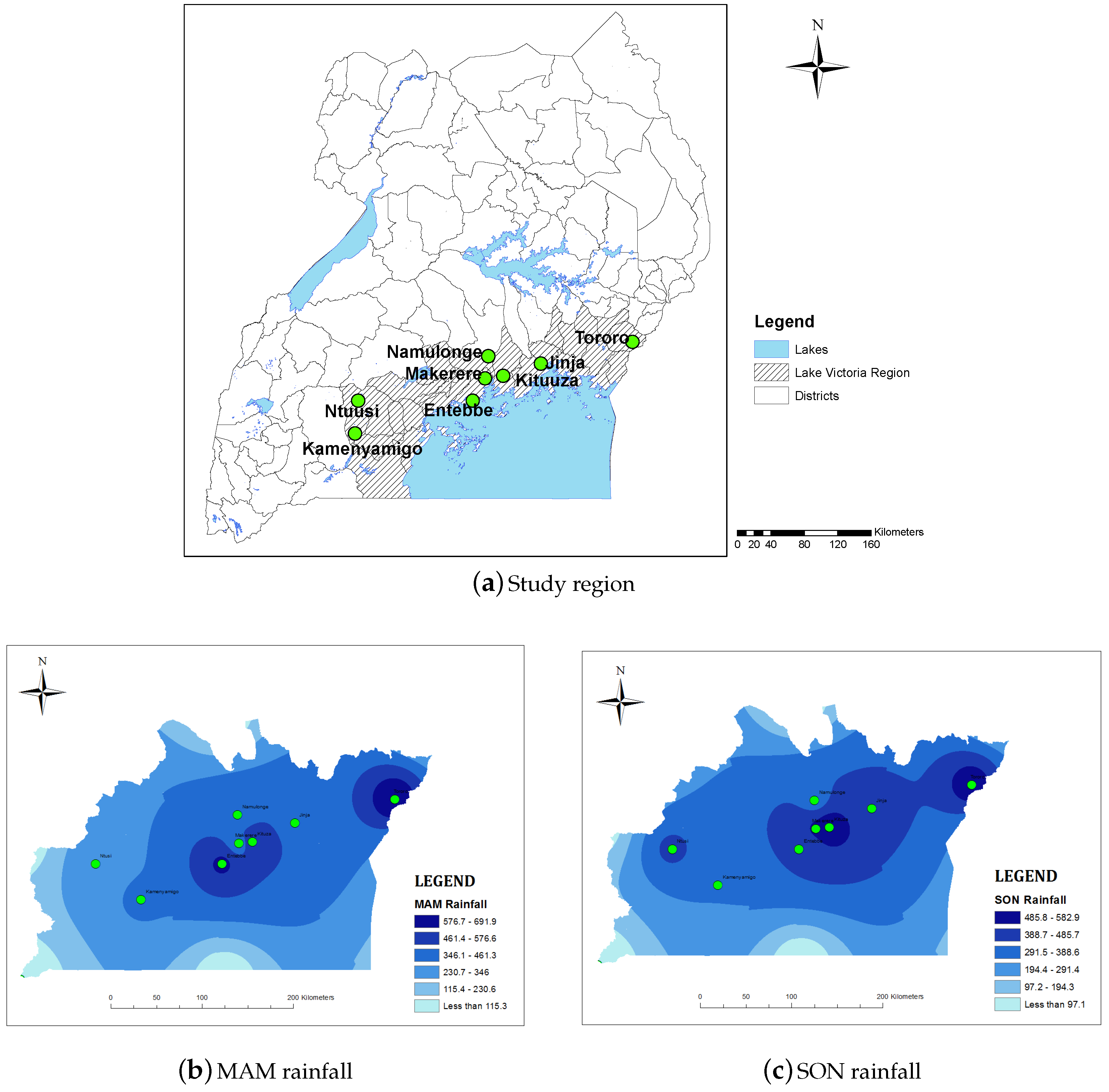
2.1. Study Area

The study was focused on the Ugandan side of Lake Victoria Basin (Figure 1a), which is found in East Africa covering three countries: Uganda, Kenya and Tanzania. Geographically, Lake Victoria spans latitudes 0.33°N–3°S and longitudes 31.67°E–34.88°E [4,6] and is the second largest lake in the world [10]. The LVB experiences annual rainfall of about 1200 mm throughout the year [5,10] generally distributed into two distinct rainfall seasons (Figure 1b,c). These seasons are March–April–May (MAM) and September–October–November (SON) , which coincide with the seasonal migration of the ITCZ. The LVB has a population of about 340 million people [6] with an annual growth rate of between 2.5% and 11.5% [20].

2.2. Data

Daily rain gauge rainfall data were obtained from the Uganda National Meteorological Authority (UNMA) for eight stations, namely Entebbe, Makerere, Namulonge, Jinja, Kituza, Ntuusi, Kamenyamigo and Tororo, drawn from the same climatological zone [21], as illustrated in Figure 1. These data are for 16 years (2000–2015) and were treated to quality control measures by testing homogeneity using the double–mass method suggested by [22,23] (Appendix A.1) and normality using Shapiro–Wilk’s test (w) described by Royston [24,25,26] (Appendix A.2). Although limitations of the double–mass curve have been discussed by Wigbout [23], it is extensively used in hydrological studies, e.g., by Tabari and Aghajanloo [27] and Sayemuzzaman and Jha [28]. The missing values in the data were filled using a simplified normal ratio method (Appendix A.3), Equation (1), which is recommended by the World Meteorology Organization (WMO) [29] and is presented as:
b i = B ¯ × a i ( A ¯ )
where b i is the missing record to be filled of station B; a i is the observed record of station A; A ¯ and B ¯ are the mean of observed records of stations A and B, respectively. The condition for using this method is that the missing records should be less than 5% of total observations, and the stations A and B should be highly correlated.
We then computed dekadal rainfall by summing up ten-day accumulated rainfall [13,30]; the total rain days over the dekads and obtained nine dekads over the entire MAM season. In order to comprehensively study rain days, the number of consecutive dry days (i.e., no rain), ‘light rain days’, ‘wet days’ and ‘days with extreme rainfall’ over the MAM season are also analyzed. The light rain day is defined by Tennant and Hewitson [31], and adopted by UNMA [32], as a day having total rainfall less than 1 mm; the wet day is defined by Kiktev et al. [33] as a day having accumulated rainfall greater than 10 mm, while days with extreme rainfall are days having total rainfall greater than the 95 percentile [34,35]. We also investigated the rainfall intensity over the dekads by using a proxy estimate computed as the ratio of accumulated dekadal rainfall to the dekadal number of rain days.

2.3. Data Analysis

The trends in rainfall were determined using the Mann–Kendall MK trend test (Appendix A.4) and simple linear regression, S L R (Appendix A.5). The M K trend test is a non-parametric test used to investigate the trends of hydro-meteorological variables. It has been used widely, e.g., by Kizza et al. [4] investigating rainfall trends over LVB and Mugume et al. [36] analyzing temperature trends over Northern China. When using the M K trend test, Zende et al. [37] suggested a null hypothesis of “there is no trend” at the 95% confidence level. If say M K < 0, the trend is considered a decreasing trend, and if M K > 0, it is considered an increasing trend. The S L R is a popular parametric trend analysis tool used in many trend studies; e.g., Lacerda et al. [38] used S L R to obtain negative precipitation trends over Northeast Brazil and Cape Verde. This combination of methods is also used by Nsubuga et al. [2] while investigating rainfall trends over western Uganda.

3. Results and Discussion

3.1. Seasonal Rainfall Amount and Rain Days for the Period 2000–2015

The average rainfall amount and the number of rain days registered during the MAM and SON seasons over LVB is presented in Table 1. It is noticeable that the total seasonal rainfall amount of MAM is marginally greater than that of SON (471 mm for MAM vis-à-vis 437 mm for SON) and on overage the same rainfall days. We also noted that the MAM season had slightly fewer light rain days and slightly more wet days than the SON season.
The rainfall data were tested for homogeneity using the double-mass curve (Figure 2) and found to be homogeneous. Tororo station experienced comparatively more rainfall than the other stations, which is illustrated by the its steep slope (i.e., the yellow line).
The gradient of the curves varies due to the spatial variation of rainfall events. Additional data quality control was inspecting the rainfall data to make sure we did not have bogus data, such as rainfall less than 0 mm. We then carried out normality tests using Shapiro–Wilk’s normality tests (w) (Table 2). The w results show that our data were homogeneous, and 65% of the dekads used had a normal distribution. The values with an asterisk (*), i.e., 35% of the dekads in Table 2, are not significant at the 95% confidence level.
We also determined the correlation of dekadal rainfall and dekadal rain days (Table 3). The results show a significant high correlation at the 95% confidence level. The high correlation coefficient (r) (i.e., r: 0.43–0.72) implies that the dekadal rainfall variability is affected by the variation of dekadal rain days and is in line with the observation by Zhai et al. [39] that the variation of total rainfall is attributed to the changes in the frequency of rain days. The exception case occurred for the sixth dekad that had a low correlation (r: 0.43) with Jinja giving a negative correlation (r: −0.57).

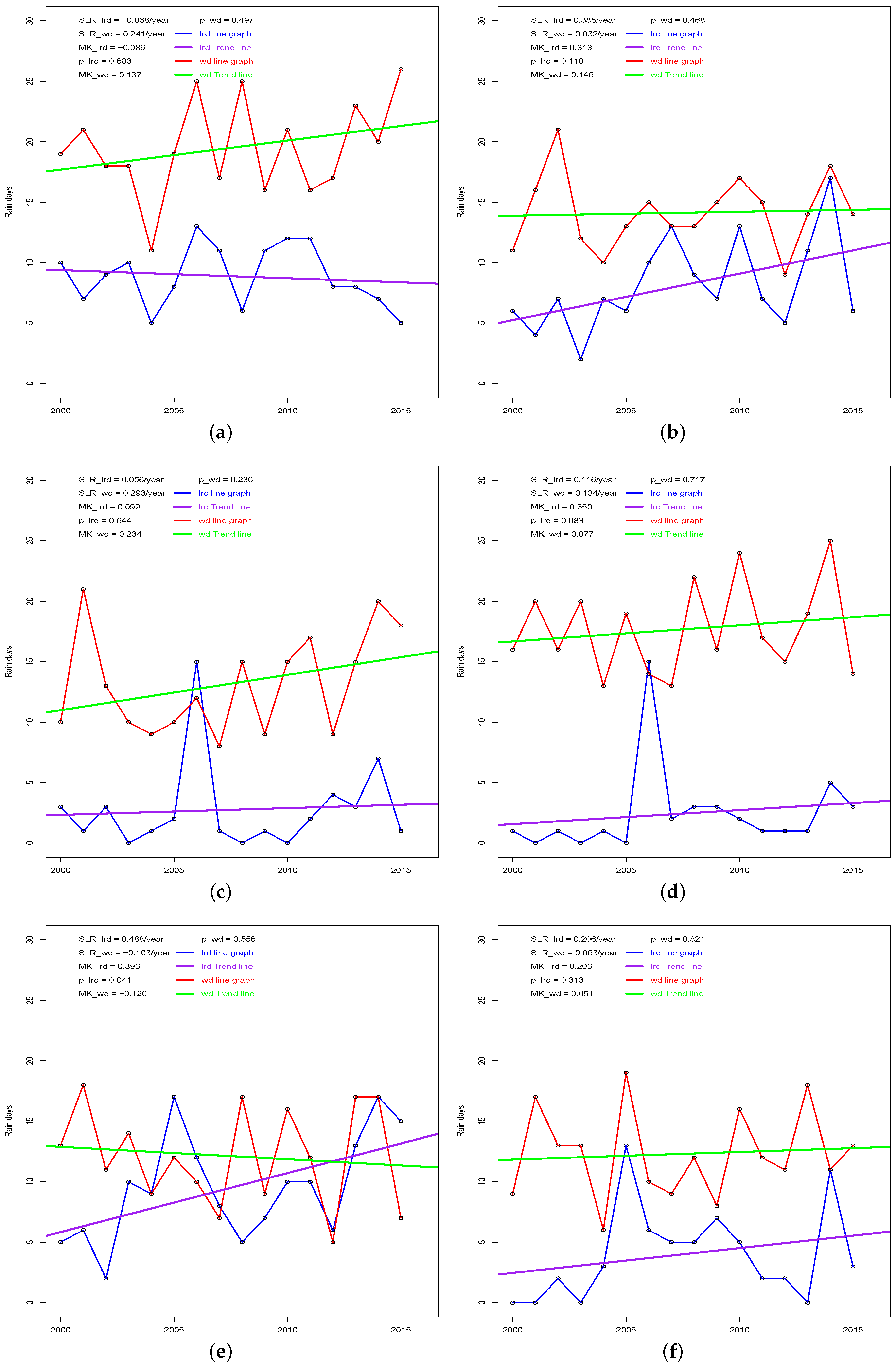
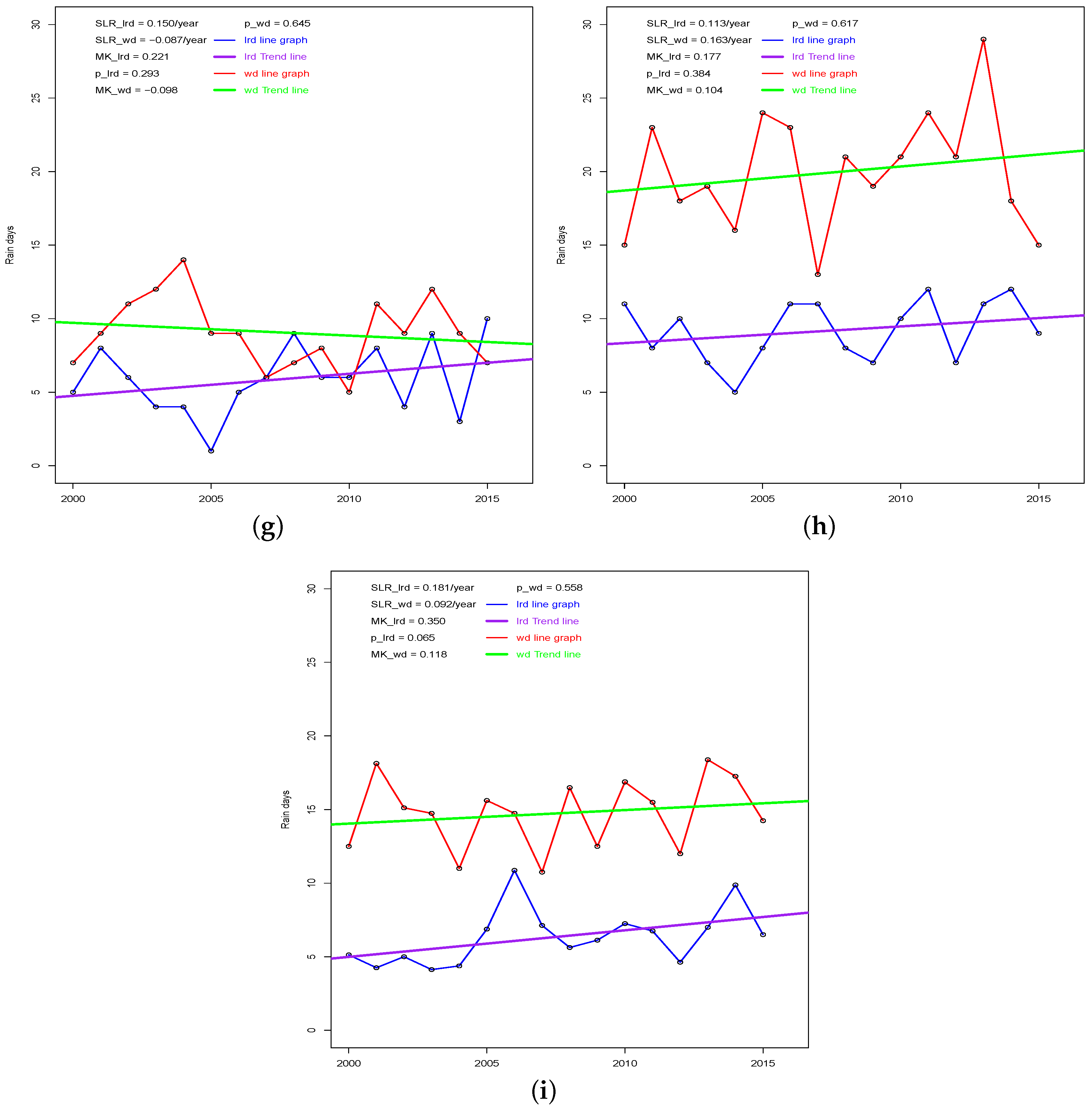
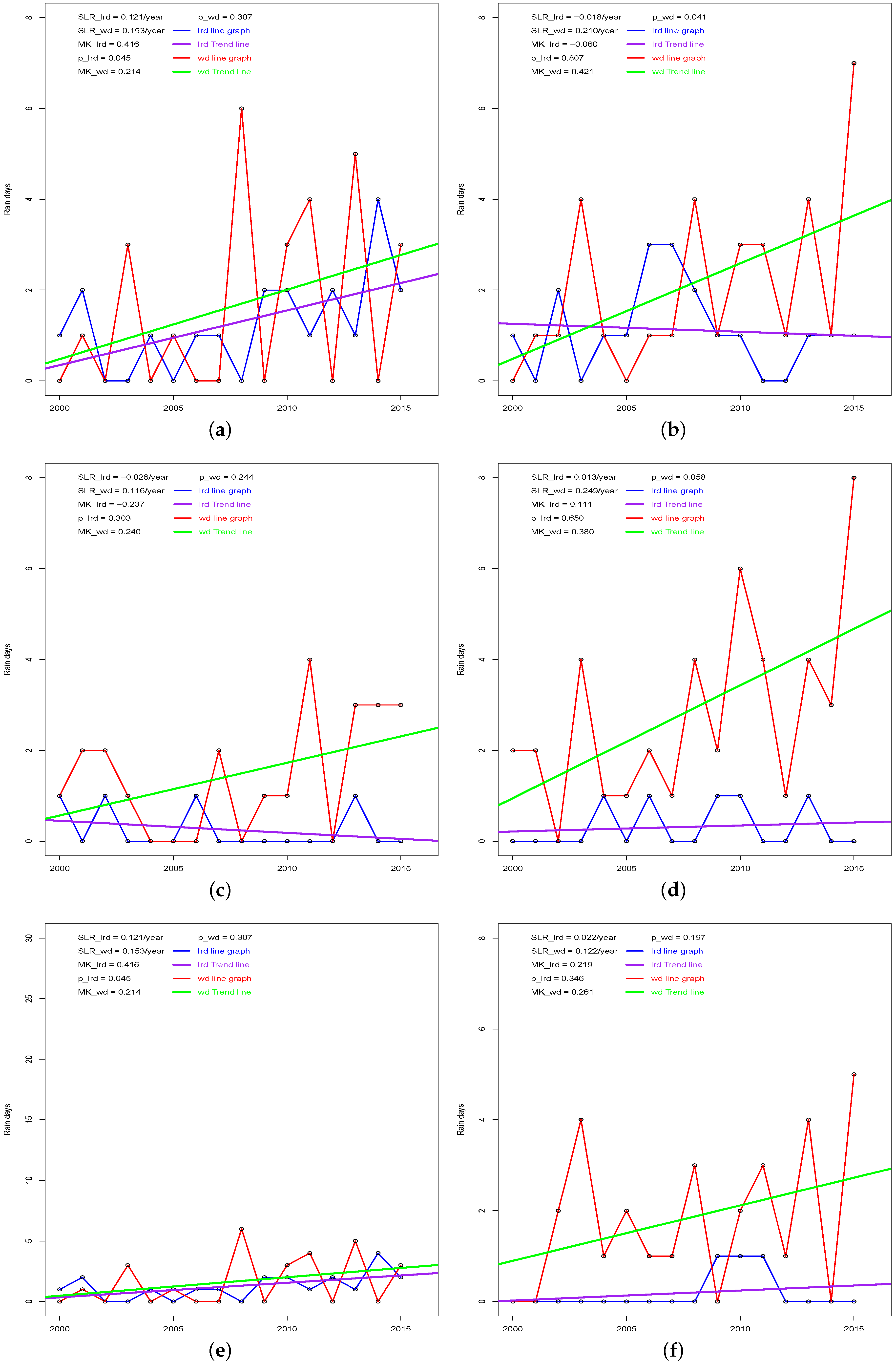
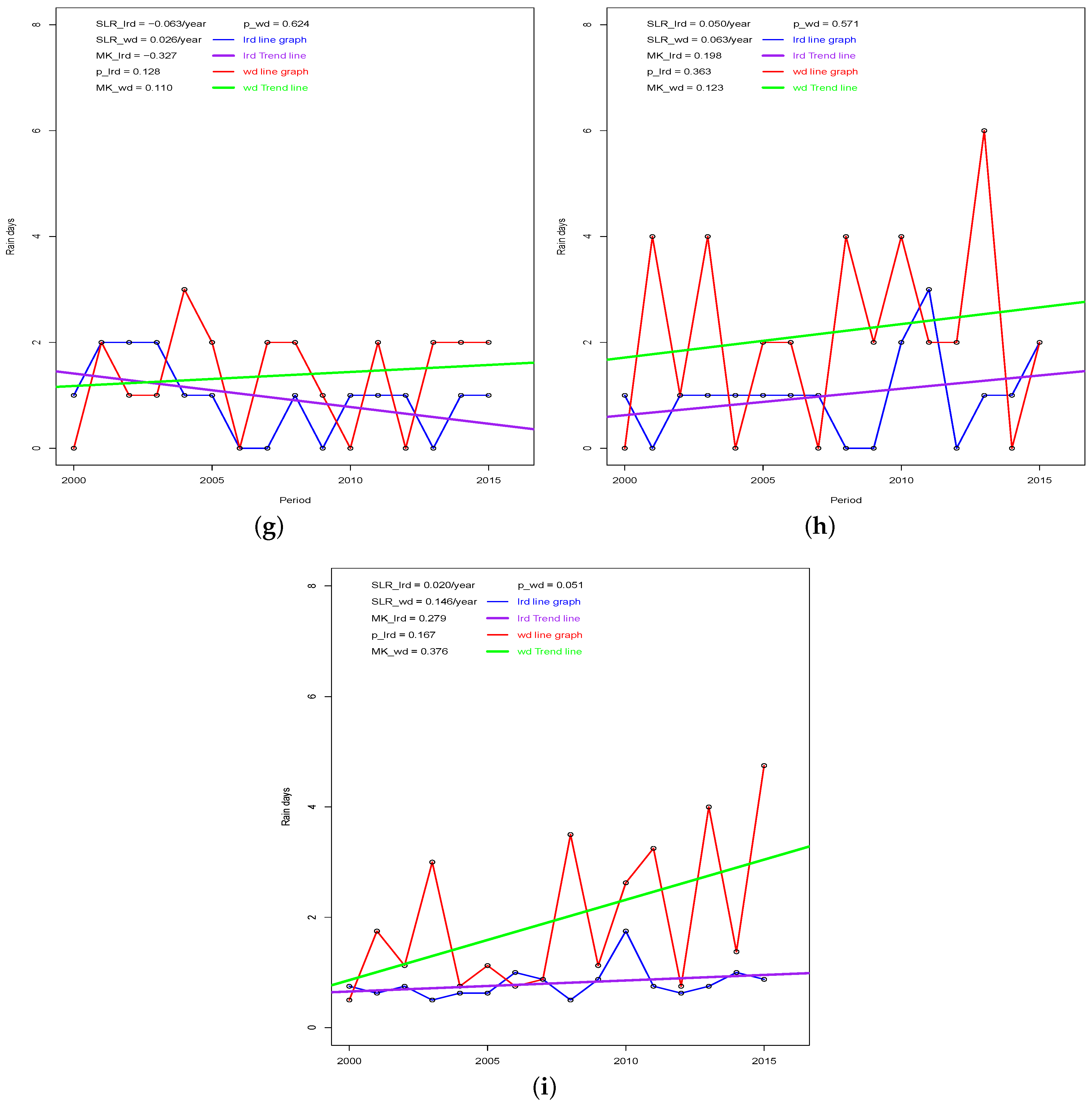
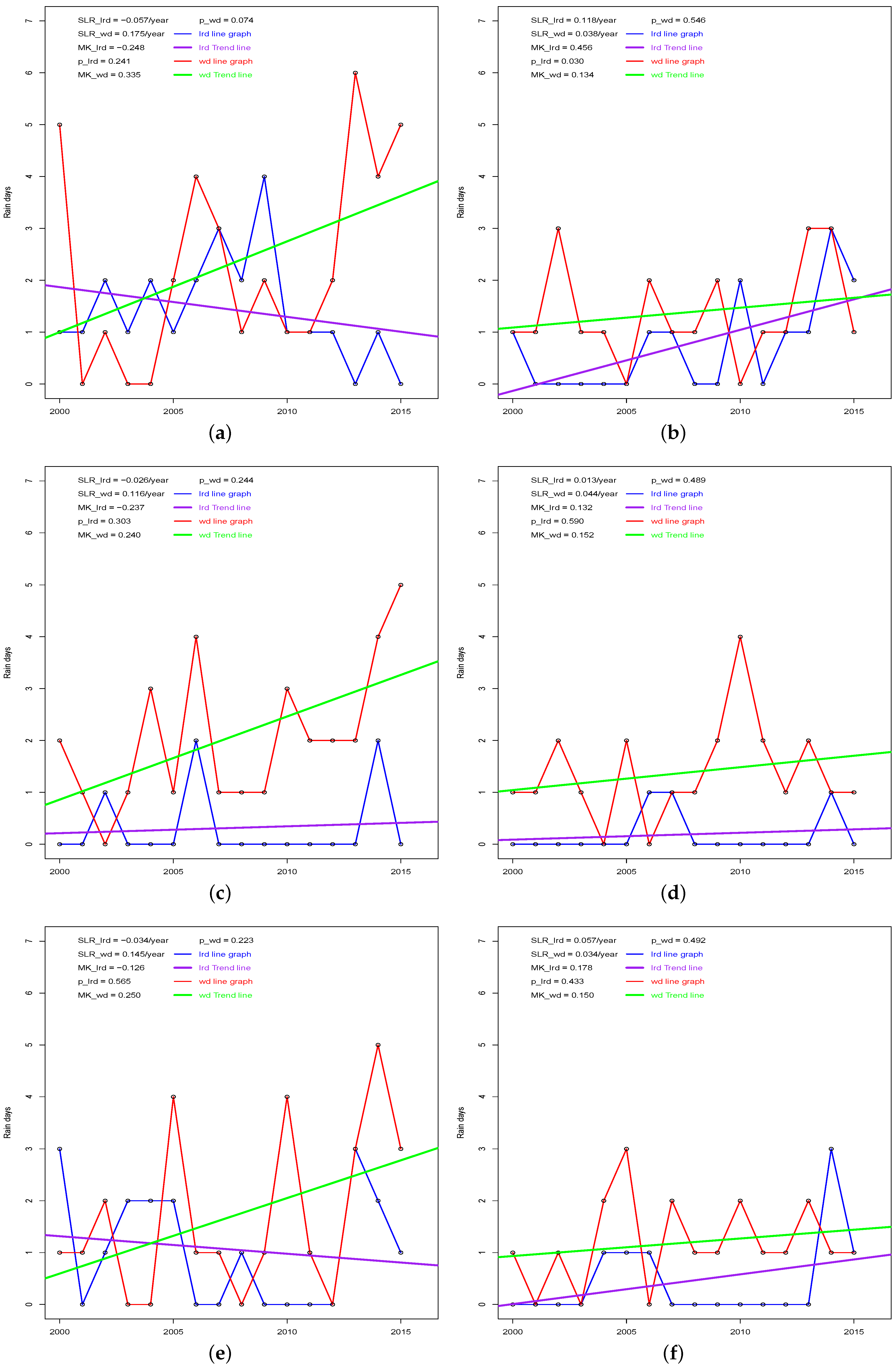
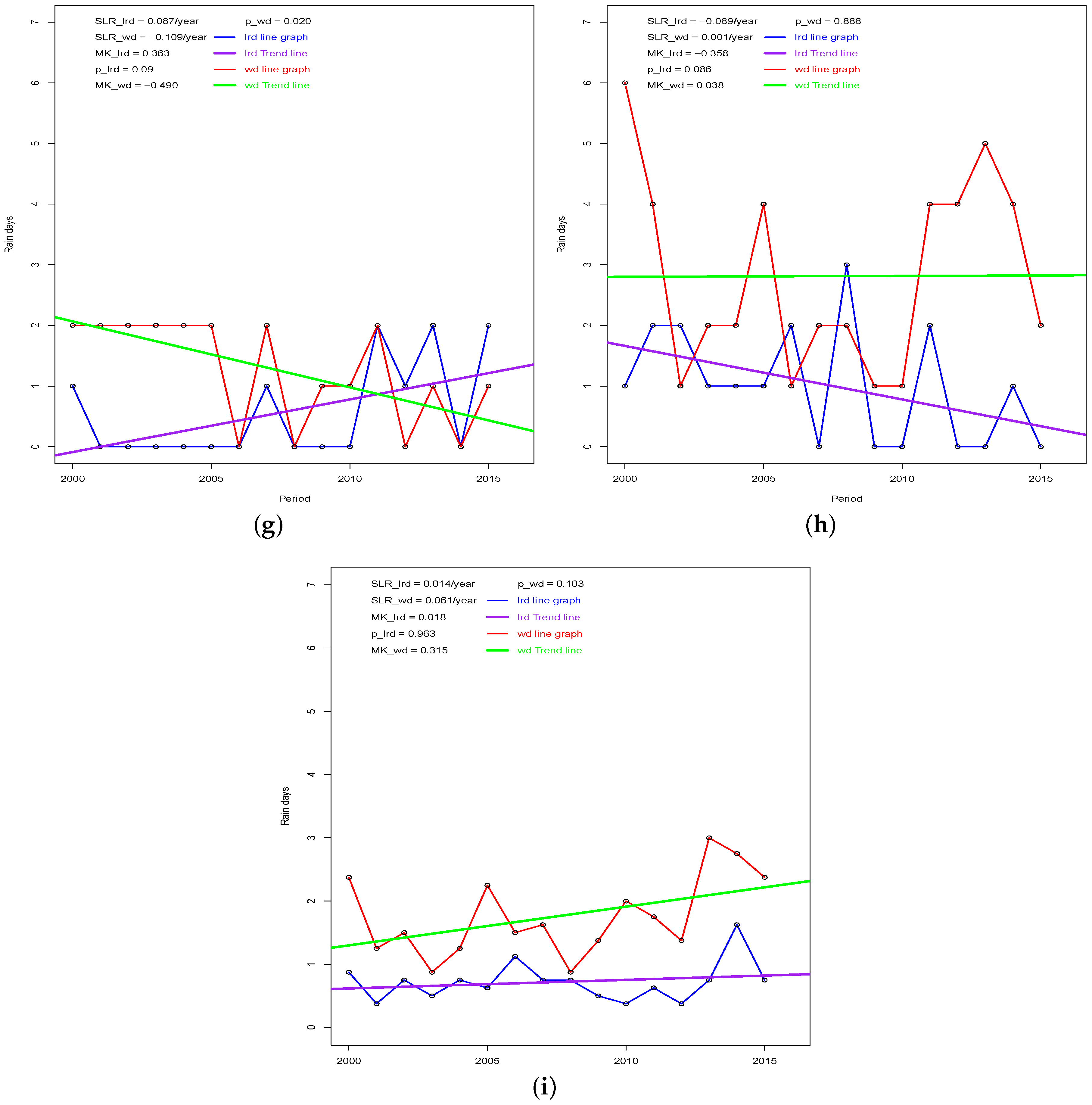
3.2. The Trend of Dekadal Rain Days

Table 4 presents the results of the M K trend of individual stations under study for the dekadal rain days. The results show that 6/8 stations in the third dekad ( M K : 0.179–0.330) had an increasing trend of dekadal rain days, which is also observed during the seventh dekad ( M K : 0.091–0.559). However, these trends were not significant at the 95% confidence level, but the small variation among the trends of individual stations (e.g., indicated by standard deviation of 0.148 for the third dekad) suggest consistency and probably demonstrate that rain days are increasing over these dekads. With the exception of Namulonge (which had 8/9 dekads with decreasing M K score), all of the other stations presented an increasing trend; increasing in the range of 0.099–0.259 days/year an average of 0.192 days/year. Further investigation of the trend of the light rain days over the MAM season (SLR; Figure 3) revealed that with the exception of Entebbe ( S L R : −0.068 per year; M K : −0.086; Figure 3a), all of the other stations had an increasing trend with an average of S L R : 0.181 per year; M K : 0.35 and p-value = 0.065. For the “wet days”, apart from Makerere ( S L R : −0.103 per year and M K : −0.120) and Ntusi ( S L R : −0.087 per year and M K : −0.098), all of other stations had an increasing trend of the MAM wet days. We obtained a general increasing trend of MAM wet days over the region ( S L R : 0.092 per year and M K : 0.118, p = 0.5576 ; Figure 3i). In general, the rate of increase of light rain days ( S L R : 0.181 per year and M K : 0.350) is twice the rate of the increase of wet days ( S L R : 0.092 per year and M K : 0.118). The increasing trend of light rain days, greater than the wet days will likely impact hydrological and agriculture sectors negatively since light rain events have little use in agriculture and hydrology.
Additional analysis of the trend of light rain days and the wet days during the third and seventh dekads is presented using Figure 4 and Figure 5, respectively. For the third dekad, only Jinja, Kamenyamigo and Ntusi had a decreasing trend of light rain days, but all other stations had an increasing trend of light rain days. For the wet days, all of the stations had an increasing trend during the third dekads. Analysis of the seventh dekad showed that Entebbe, Kamenyamigo, Makerere and Tororo had a decreasing trend of rain days. For the wet days, only Ntusi had a decreasing trend. Generally, for the third dekad, the rate of increase of light rain days ( S L R : 0.020 per year and M K : 0.279) is slightly smaller than the rate of increase of wet days ( S L R : 0.146 per year and M K : 0.376), which was also noted for the seventh dekad (wet days: S L R = 0.061 per year; M K = 0.315 and rain days: S L R = 0.014 per year; M K = 0.018).
Rain days have profound importance to agricultural production [40], and the decreasing trend of rain days during the first and the second dekads can have a negative impact on the onset of seasonal rainfall. It can create a serious shortage of available soil water to support crop germination [41], thus rendering a late start of the season. The change in rain days can also impact the presence and severity of dry spells or drought within a given season. If a severe dry spell occurs during the flowering period, e.g., during the 5th–6th dekad (which is considered to have a peak rainfall regarding the MAM season by Camberlin et al. [42]), caused by a decreasing number of rain days over the same period, crop loss may result [43]. The actual severe impact will depend on the available water in the soil, especially the water holding capacity of the soil in question [11,43]. The decreasing number of dekadal rain days during the ninth dekad can have a positive impact during the harvesting period and even lead to a reduction in post-harvest losses [44].

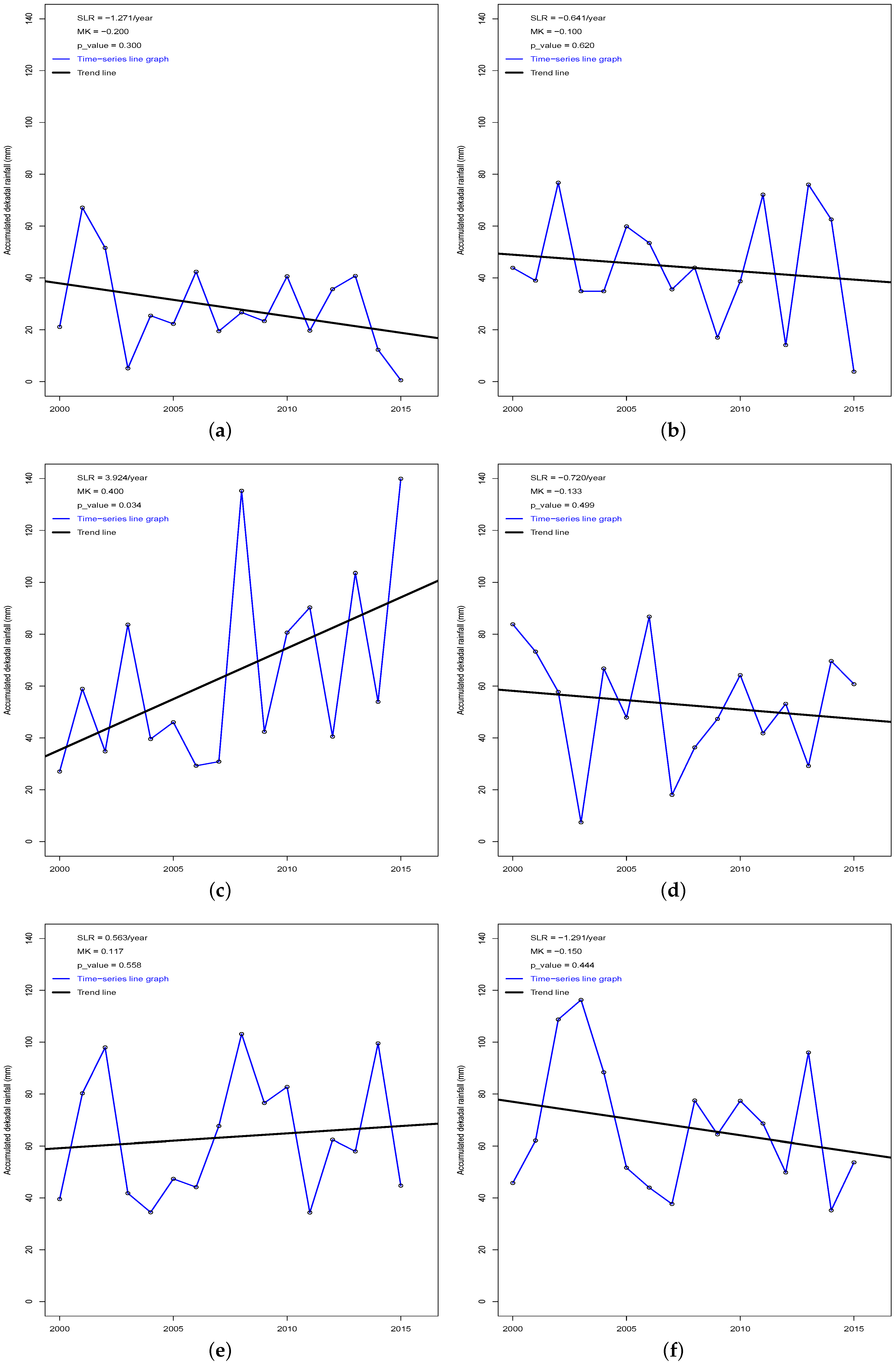
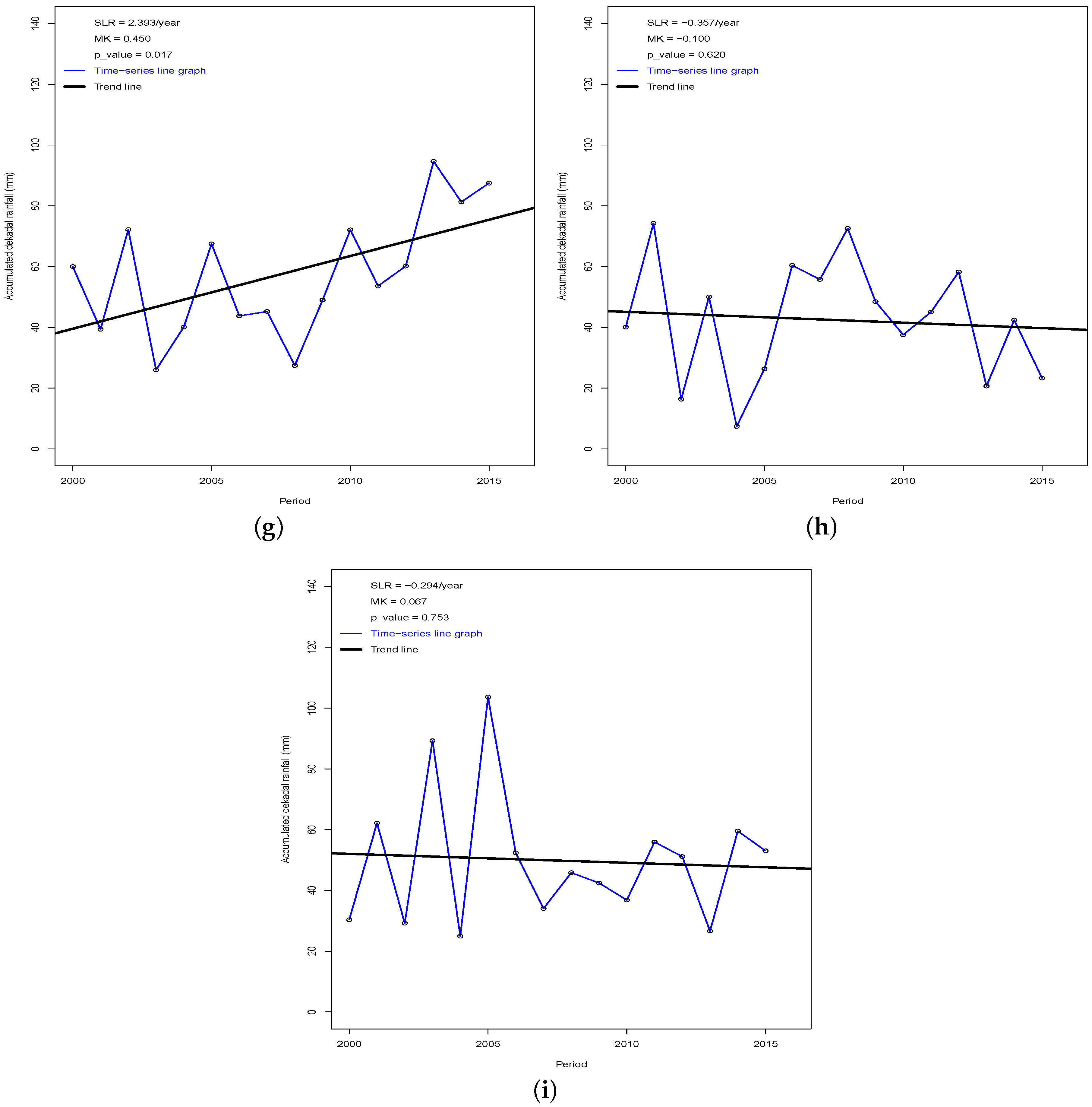
3.3. The Trend of the Dekadal Rainfall Amount

The general time-series trend of dekadal rainfall over the LVB is presented using Figure 6 by averaging the daily rainfall of individual stations. The results of S L R and the M K trend were put inside the respective figure. We noted that the average dekadal rainfall over the third and the seventh dekads is increased at S L R : 3.924 and 2.393 per year, respectively. The M K trend also showed an increasing trend, significant at the 95% confidence level with the third and seventh increasing at M K : 0.400 and p-value = 0.034 (Figure 6c) and M K : 0.450 and p-value = 0.017 (Figure 6g), respectively. Additional results of the M K trend for each station are presented using Table 5.
The S L R results are in line with the M K trend results, and the dekadal rainfall trend of individual stations was increasing at 0.25–5.48 mm annually for each of the MAM seasons, aggregating to an average of 2.62 mm annually. We also noted an insignificant decreasing trend in dekadal rainfall amount during the first ( M K : −0.158; S L R : −1.271 mm/year), second ( M K : −0.101; S L R : −0.641 mm/year) and sixth ( M K : −0.097; S L R : −1.291 mm/year) dekads. This probably implies a decrease in rainfall intensity over the dekads identified and an increase in wetness over the third and seventh dekads. This view of increased wetness over a given period was pointed out by Zende et al. [37] while studying the rainfall trend over a semi-arid region of India, but they used monthly rainfall totals.
The decreasing rainfall amount during the first and second dekads can impact negatively the onset of the MAM season, as there will be less moisture to support crop germination [40,45,46], yet on-set is important regarding the performance of MAM rains over East Africa [45]. However, Mugalavai et al. [46] found no significant shift in MAM seasonal rainfall on-set and cessation over LVB during the last century, and Awange et al. [6] noted that spatial and temporal rainfall patterns have not changed appreciably over LVB for the period 1998–2012. The noted variations of dekadal rainfall can therefore be attributed to the variability of mesoscale systems. These results of varying dekadal rainfall are consistent with the variation of dekadal rain days over the same period described in Section 3.3.

3.4. The Dekadal Rainfall Intensity

Table 6 presents the results of the M K trend for the dekadal rainfall intensity defined in Section 2.2. We did not compute the S L R trend since dekadal rainfall intensity is a derived proxy parameter, yet S L R being a parametric tool requires actual values. For the third and seventh dekads, 6/8 stations had increase trend of dekadal rainfall intensity in the range of M K : 0.150–0.276 and M K : 0.033–0.317, respectively. Since both dekadal rainfall and dekadal rain days are increasing during the third and seventh dekads, these results probably suggest that the dekadal rainfall is increasing at a slightly greater rate compared to the dekadal rain days. We also noted a decreasing trend of dekadal rainfall intensity during the first dekad ( M K : −0.276 to −0.019) with the exception of Ntusi and the sixth dekad ( M K : −0.219 to −0.010) with the exception of Kamenyamigo, and we had earlier noted a decreasing trend of dekadal rainfall (Section 3.3) and dekadal rain days (Section 3.2) during the same period, which make us confirm a decreasing trend of dekadal rainfall since dekadal rainfall and dekadal rain days are positively correlated (r: 0.63 and 0.43, respectively).

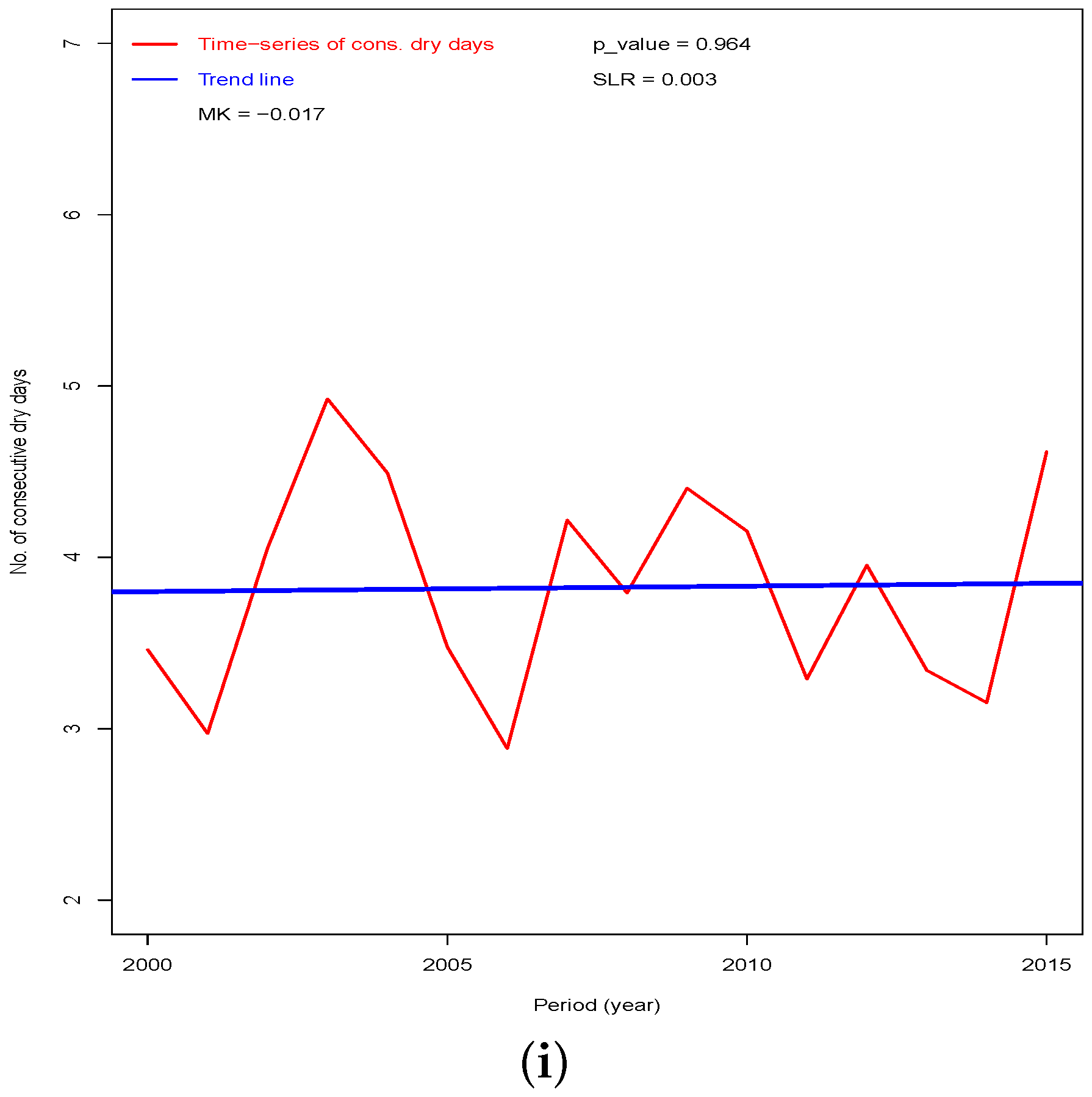
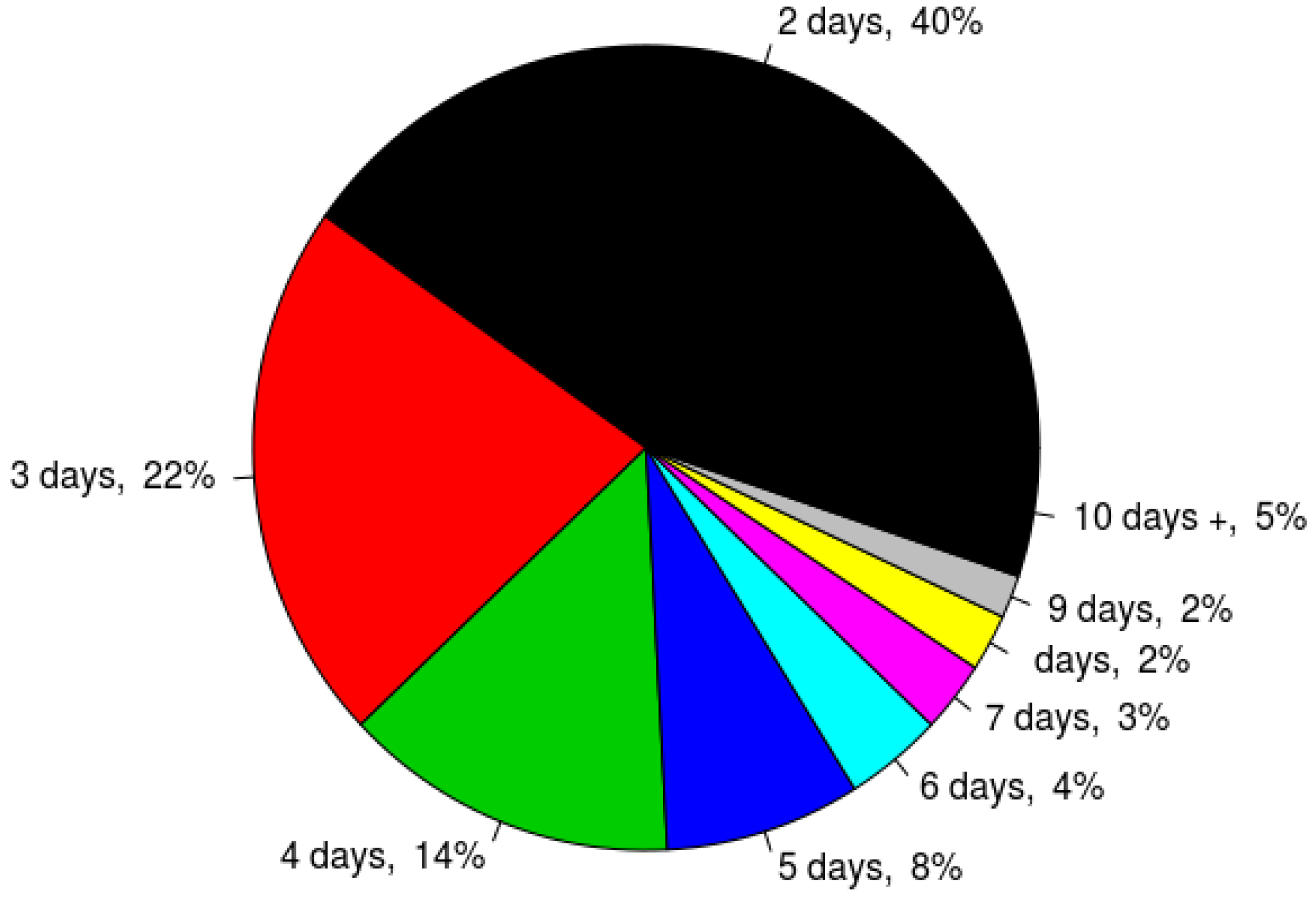
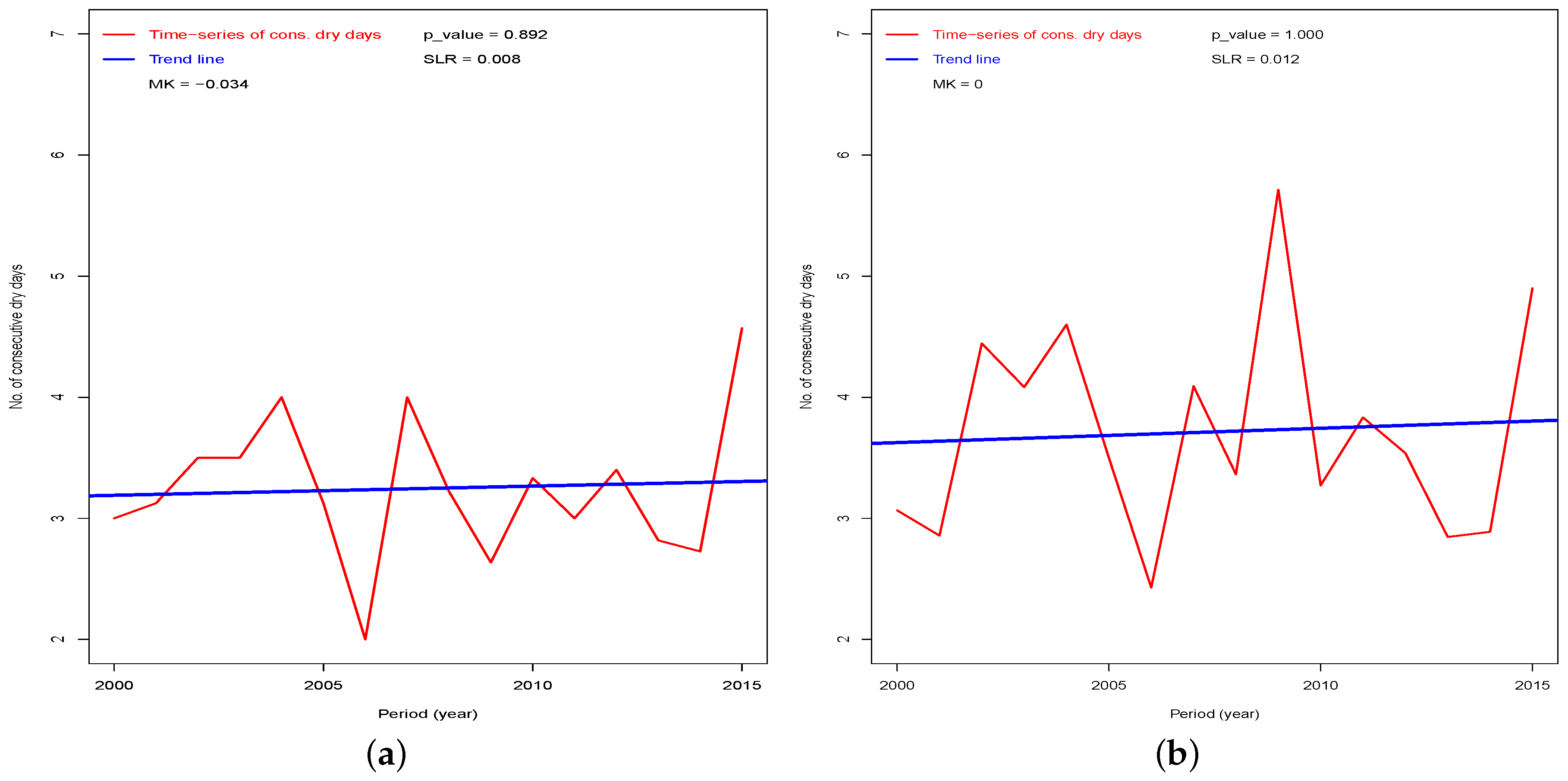
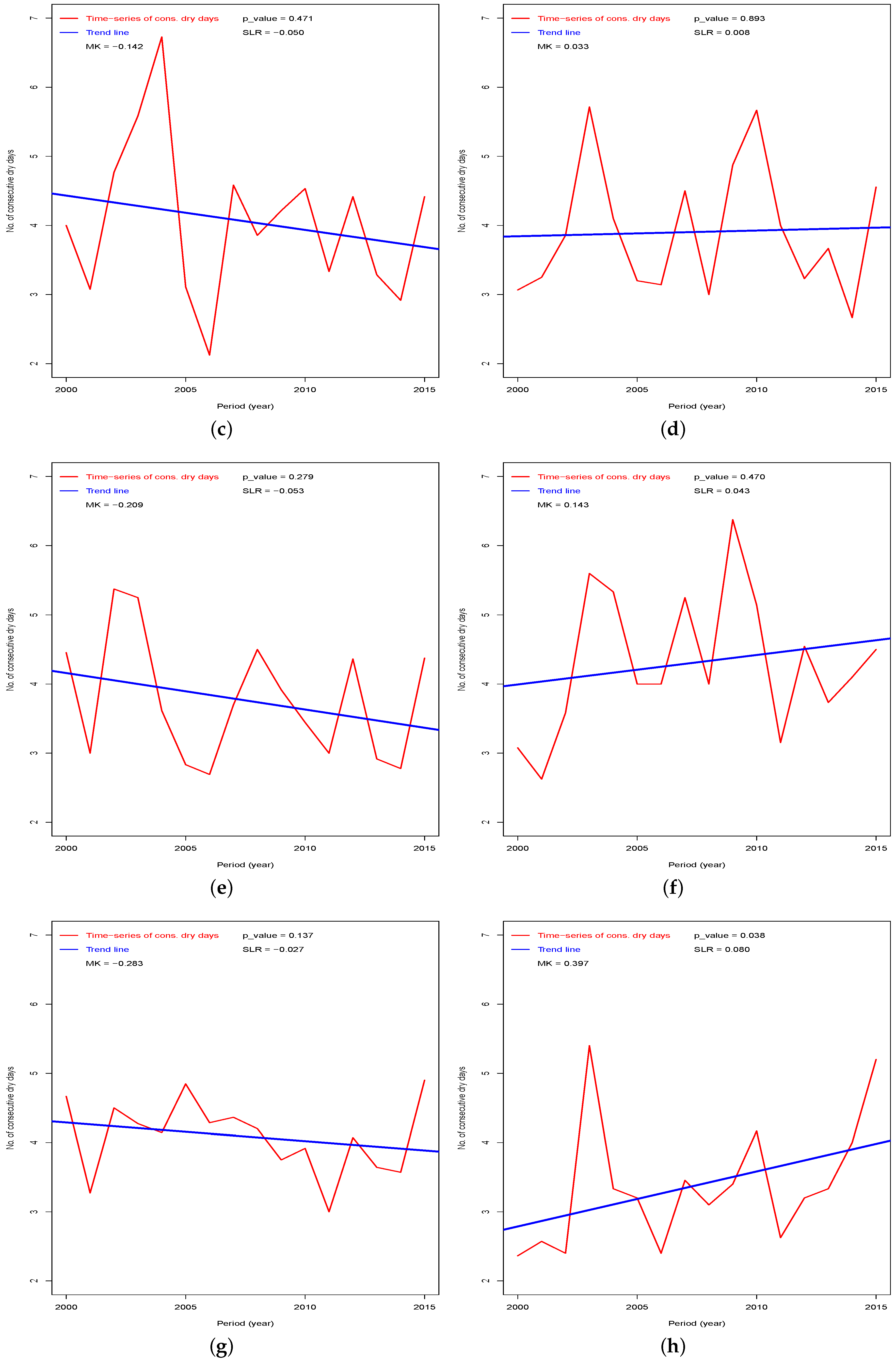
3.5. The Trend of Extreme Weather

The results for the trend of consecutive dry days during the MAM season of 2000–2015 are presented using Table 7 and Figure 7 and Figure 8. Table 7 shows the absolute number of consecutive dry days for each station over 2000–2015; Figure 7 shows the seasonal average number of consecutive dry days for each station per year; while Figure 8 shows the percentage number of the consecutive dry days over the study period. The results show that there was more frequent short dry spells with 2 days, 3 days and 4 days of consecutively no rain forming 40%, 22% and 14%, respectively (Figure 8). We noted that Jinja ( M K : 0; S L R : 0.012), Kituza ( M K : 0.033; S L R : 0.008), Namulonge ( M K : 0.143; S L R : 0.043) and Tororo ( M K : 0.397; S L R : 0.080) had increasing trends and that Tororo’s trend was increased significantly at 90%, and since we found that Tororo could have experienced more rainfall in Section 3.1, it could probably indicate an increased frequency of consecutive dry days with occasional heavy rainfall. The other stations had decreasing trends, and we also found a general non-significant decreasing trend (Figure 7i) on aggregating all of the stations ( M K : −0.017; S L R : 0.003 and p-value: 0.964). The increasing trend of consecutive dry days has implications for dry spells [47] within a given season. The dry spells can result in meteorological drought whose effects can cascade, affecting agriculture and hydrology negatively.
The M K trend results for extreme rainfall over the study region are presented in Table 8. The values with an asterisk (*) and a double asterisk (**) are significant at the 90% and 95% significance levels, respectively. We noted that during the third dekad, 6/8 stations had an increasing trend, while 7/8 stations had an increasing trend during the seventh dekad. On aggregating the dekads, results indicated that extreme rainfall is increasing significantly during the third and seventh dekads compared to the overall season.

4. Summary and Conclusions

The main aim of our study was to investigate the intra-seasonal rainfall variability over LVB by analyzing dekadal rainfall. The daily rainfall obtained from UNMA was first treated to the normality test using Shapiro–Wilk’s normality test and homogeneity test using double-mass curves. Sixty five percent of the data was found normally distributed at the 95% confidence level, and all stations had homogeneous rainfall data records. The missing rainfall data were less than 5% and filled using the modified normal ratio method. The rainfall data were then classified in dekads from which dekadal rainfall amount and dekadal rain days were computed. The average rainfall and rain days during the March–May and September–November seasons over LVB was almost similar in magnitude, and we also noted that the March–May season had fewer light rain days and more wet days than the September–November season.
The trend of accumulated rainfall and the total number of rain days over a given dekad were analyzed using the Mann–Kendall trend test and simple linear regression and presented using tables and figures. The majority of the trends were generally not significant at the 95% confidence level, but consistent and pointed to an increasing trend in both accumulated rainfall and total number of rain days during the third and seventh dekads and decreasing trends during the 1st, 2nd and 6th dekads. We also noted a greater and significant increase of dekadal rainfall of the seventh dekad compared to the third dekad over the last ten years (2006–2015) and a corresponding significant decrease in dekadal rainfall during the eight dekad.
Additionally, we found that the trend of light rain days was generally twice as much as the increase of wet days, which was also evident during the third and seventh dekads. We also analyzed the trends of dekadal rainfall intensity and found them consistent with earlier results showing increasing trends during the third and seventh dekads and decreasing trends for the first and sixth dekads. Analysis of consecutive dry days showed that 2–4 days with consecutively no rainfall accounted for 74%, and we did not find a significant trend. The days with extreme rainfall increased significantly during the third and seventh dekads. Since other studies over the same region have pointed to a ‘no significant change’ in March–May seasonal rainfall regarding on-set and cessation, our results suggest intra-seasonal shift in March–May seasonal rainfall, making the third and seventh dekads become wetter.

Acknowledgments

The authors are grateful to the WIMEA-ICTproject for the support and to the reviewers for the constructive feedback. We are also grateful to UNMA for availing the rainfall data used in the study. The authors also acknowledge the help of Romano Ssembajwe and Daniel Kisitu for the graphics.

Author Contributions

Isaac Mugume, Godfrey Mujuni, and Triphonia Jacob Ngailo conceived, designed and carried out the study under the guidance and supervision of Michel d.S. Mesquita, Charles Basalirwa, Daniel Waiswa and Joachim Reduer. Alex Nimusiima, Yazidhi Bamutaze and Sulin Tao discussed the results.

Conflicts of Interest

The authors declare no conflict of interest.

Appendix A.

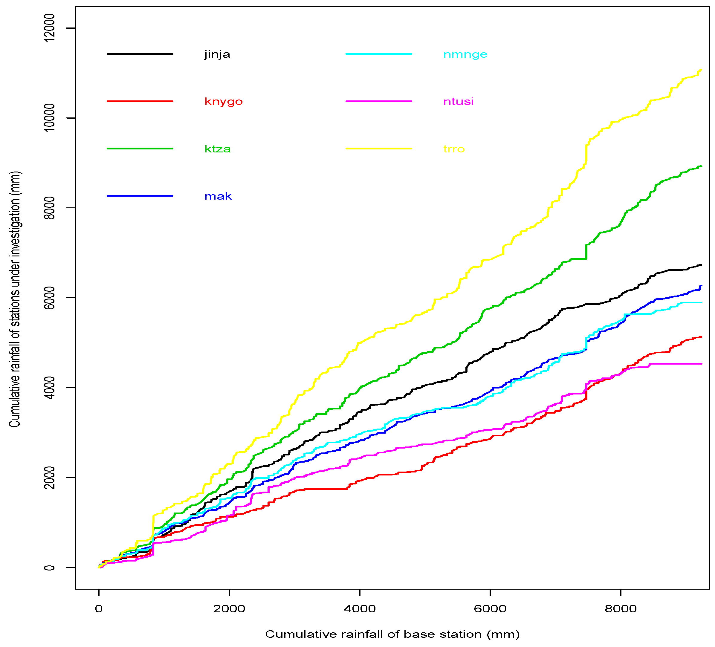
Appendix A.1. The Double-Mass Curve

Given two datasets:
y = y 1 , y 2 , , y n
and
x = x 1 , x 2 , , x n
such that Y and X are the cumulative values of y and x, respectively, and that:
Y i = i = 1 n y i
and
X i = i = 1 n x i
the graph of a curve passing through the coordinate ( X i , Y i ) is a double-mass curve [23]. We used “ebb” as the reference dataset.

Appendix A.2. Shapiro–Wilk’s Normality Test

Given dekadal rainfall data:
R 1 , R 2 , , R n
from which we get an order data:
R ( 1 ) , R ( 2 ) , , R ( n )
Shapiro–Wilk’s statistic tests normality by using a null hypothesis of ‘the population is normally distributed’. We use the Shapiro–Wilk (w) test statistic as:
w = i = 1 n α i R ( i ) 2 i = 1 n ( R ( i ) R ¯ i ) 2
where R i is the smallest i-th dekadal rainfall value, R ¯ i is the mean dekadal rainfall computed using:
w = 1 n i = 1 n R i
and α i constants depending on expected values of order statistics from a standard normal distribution. The values of w are such that:
0 < w < 1
with values of w closer to one indicating high normality.

Appendix A.3. The Normal Ratio Method

According to Subramanya [48], given a rainfall time-series,
R 1 , R 2 , , R n
with normal rainfall within 10% of a station with missing rainfall R i , the rainfall, R i can be estimated by:
R i = ( R i ¯ ) N R 1 ( R 1 ¯ ) + R 2 ( R 2 ¯ ) + + R n ( R n ¯ )
where R j ¯ is the j-th mean rainfall for the period under consideration and N is the number of stations used. For daily rainfall, we can take a station with high correlation to help estimate the rainfall of a missing station. If we simplify and take one station (i.e., N = 1 ) with the highest correlation to estimate the missing rainfall, Equation (A5) becomes:
R i = R i ¯ × R 1 ( R 1 ¯ )
Equation (A6) is used to estimate missing rainfall values as Equation (1) with two conditions that (1) the station with missing data is highly correlated with the station having all of the data and (2) the missing data should be less than 5%.

Appendix A.4. The Mann–Kendall Trend Test

The M K test is a sign test for detecting trends in stationery hydro-meteorological variables. The sign (S) is obtained using Equations (A7) and (A8) and following the algorithm written by McLeod [49].
S = i = 1 n 1 j + i = 1 n s g n ( R j R i )
where R i and R j are rainfall amounts (or rain days) sequentially, and s g n ( R j R i ) is obtained as:
s g n ( R j R i ) = + 1 : if R j R i > 0 0 : if R j R i = 0 1 : if R j R i < 0
For non-tied values of R i , the variance δ 2 ( S ) of the distribution of S is computed using:
δ 2 ( S ) = n ( n 1 ) ( 2 n + 5 ) 18
For tied values of R i , the variance is given by:
δ 2 ( S ) = n ( n 1 ) ( 2 n + 5 ) t i ( i ) ( i 1 ) ( 2 i + 5 ) 18
t i is number of ties of extent i. The M K test statistic is then given by the standard Gaussian value, M K defined as:
M K = S 1 δ ( S ) : if S > 0 0 : if S = 0 S + 1 δ ( S ) : if S < 0

Appendix A.5. Regression Analysis

Linear regression is a simple method for determining the trends of time-series data [41]. Given an n time-ordered rainfall (rain days) dataset: { R 1 , R 2 , , R n 1 , R n }, ordered in time, t the simple linear regression is given as (A12):
R i = α t i + ε
where
i = 1 , 2 , , n
α is the rate of change, ε is the error and the decadal rate of change of rainfall (rain days) over the study period and α is the gradient of the regression line.

References

  1. Ogwang, B.A.; Guirong, T.; Haishan, C. Diagnosis of September–November drought and the associated circulation anomalies over Uganda. Pak. J. Meteorol. 2012, 9, 11–24. [Google Scholar]
  2. Nsubuga, F.N.W.; Olwoch, J.M.; Rautenbach, C.J.; Botai, O.J. Analysis of mid-twentieth century rainfall trends and variability over southwestern Uganda. Theor. Appl. Climatol. 2014, 15, 53–71. [Google Scholar] [CrossRef]
  3. Ongoma, V.; Guirong, T.; Ogwang, B.A.; Ngarukiyimana, J.P. Diagnosis of seasonal rainfall variability over east africa: A case study of 2010–2011 drought over Kenya. Pak. J. Meteorol. 2015, 11, 13–21. [Google Scholar]
  4. Kizza, M.; Rodhe, A.; Xu, C.Y.; Ntale, H.K.; Halldin, S. Temporal rainfall variability in the lake victoria basin in east africa during the twentieth century. Theor. Appl. Climatol. 2009, 98, 119–135. [Google Scholar] [CrossRef]
  5. Anyah, R.O.; Semazzi, F.H.; Xie, L. Simulated physical mechanisms associated with climate variability over lake Victoria basin in East Africa. Mon. Weather Rev. 2006, 134, 3588–3609. [Google Scholar] [CrossRef]
  6. Awange, J.; Anyah, R.; Agola, N.; Forootan, E.; Omondi, P. Potential impacts of climate and environmental change on the stored water of lake Victoria basin and economic implications. Water Resour. Res. 2013, 49, 8160–8173. [Google Scholar] [CrossRef]
  7. Mailu, A.M. Biological and integrated control of water hyacinth, eichhornia crassipes. ACIAR Proc. 2001, 102, 130–139. [Google Scholar]
  8. Sabiiti, G.; Ininda, J.M.; Ogallo, L.; Opijah, F.; Nimusiima, A.; Otieno, G.; Ddumba, D.S.; Nanteza, J.; Basalirwa, C. Empirical relationships between banana yields and climate variability over Uganda. J. Environ. Agric. Sci. 2016, 7, 3–13. [Google Scholar]
  9. Mukwaya, P.I.; Sengendo, H.; Lwasa, S. Enhancing security and resilience of low-income communities to climate change in growing cities: An assessment of flood management and planning regimes in Kampala City, Uganda. In Climate Change, Human Security and Violent Conflict; Scheffran, J., Brzoska, M., Brauch, G., Link, M.P., Schilling, J., Eds.; Springer: Berlin/Heidelberg, Germany, 2012; pp. 543–557. [Google Scholar]
  10. Williams, K.; Chamberlain, J.; Buontempo, C.; Bain, C. Regional climate model performance in the lake Victoria basin. Clim. Dynam. 2015, 44, 1699–1713. [Google Scholar] [CrossRef]
  11. Barron, J.; Rockström, J.; Gichuki, F.; Hatibu, N. Dry spell analysis and maize yields for two semi-arid locations in East Africa. Agric. For. Meteorol. 2003, 117, 23–37. [Google Scholar] [CrossRef]
  12. Goswami, B.; Venugopal, V.; Sengupta, D.; Madhusoodanan, M.; Xavier, P.K. Increasing trend of extreme rain events over India in a warming environment. Science 2006, 314, 1442–1445. [Google Scholar] [CrossRef] [PubMed]
  13. Cheung, W.H.; Senay, G.B.; Singh, A. Trends and spatial distribution of annual and seasonal rainfall in Ethiopia. Int. J. Climatol. 2008, 28, 1723–1734. [Google Scholar] [CrossRef]
  14. Nimusiima, A.; Basalirwa, C.; Majaliwa, J.; Mbogga, S.; Mwavu, E.; Namaalwa, J.; Okello-Onen, J. Analysis of future climate scenarios over central Uganda cattle corridor. J. Earth Sci. Clima. Chang. 2014, 2014, 1–13. [Google Scholar]
  15. Bowden, J.H.; Semazzi, F.H. Empirical analysis of intraseasonal climate variability over the Greater Horn of Africa. J. Clim. 2007, 20, 5715–5731. [Google Scholar] [CrossRef]
  16. Hartter, J.; Stampone, M.D.; Ryan, S.J.; Kirner, K.; Chapman, C.A.; Goldman, A. Patterns and perceptions of climate change in a biodiversity conservation hotspot. PLoS ONE 2012, 7, 1–12. [Google Scholar] [CrossRef] [PubMed]
  17. Nimusiima, A.; Basalirwa, C.; Majaliwa, J.; Otim-Nape, W.; Okello-Onen, J.; Rubaire-Akiiki, C.; Konde-Lule, J.; Ogwal-Byenek, S. Nature and dynamics of climate variability in the uganda cattle corridor. Afr. J. Environ. Sci. Technol. 2013, 7, 770–782. [Google Scholar] [CrossRef]
  18. Chaves, L.F.; Satake, A.; Hashizume, M.; Minakawa, N. Indian ocean dipole and rainfall drive a moran effect in east africa malaria transmission. J. Infect. Dis. 2012, 205, 1885–1891. [Google Scholar] [CrossRef] [PubMed]
  19. Tao, S.; Shen, S.; Li, Y.; Wang, Q.; Gao, P.; Mugume, I. Projected crop production under regional climate change using scenario data and modeling: Sensitivity to chosen sowing date and cultivar. Sustainability 2016, 8, 214. [Google Scholar] [CrossRef]
  20. Odada, E.O.; Ochola, W.O.; Olago, D.O. Drivers of ecosystem change and their impacts on human well-being in Lake Victoria basin. Afr. J. Ecol. 2009, 47, 46–54. [Google Scholar] [CrossRef]
  21. Basalirwa, C. Delineation of uganda into climatological rainfall zones using the method of principal component analysis. Int. J. Climatol. 1995, 15, 1161–1177. [Google Scholar] [CrossRef]
  22. Searcy, J.K.; Hardison, C.H. Double-mass curves. In Manual of Hydrology: Part 1. General Surface-Water Techniques; Pecora, W.T., Ed.; USA Department of Interior: Washington, DC, USA, 1960; pp. 33–64. [Google Scholar]
  23. Wigbout, M. Limitations in the use of double-mass curves. J. Hydrol. 1973, 12, 132–138. [Google Scholar]
  24. Royston, J.P. Algorithm as 181: The w test for normality. J. R. Stat. Soc. Ser. C Appl. Stat. 1982, 31, 176–180. [Google Scholar] [CrossRef]
  25. Royston, J.P. An extension of shapiro and wilk’s w test for normality to large samples. J. R. Stat. Soc. Ser. C Appl. Stat. 1982, 31, 115–124. [Google Scholar] [CrossRef]
  26. Royston, J.P. Remark as R94: A remark on algorithm as 181: The w-test for normality. J. R. Stat. Soc. Ser. C Appl. Stat. 1995, 44, 547–551. [Google Scholar] [CrossRef]
  27. Tabari, H.; Aghajanloo, M.B. Temporal pattern of aridity index in iran with considering precipitation and evapotranspiration trends. Int. J. Climatol. 2013, 33, 396–409. [Google Scholar] [CrossRef]
  28. Sayemuzzaman, M.; Jha, M.K. Seasonal and annual precipitation time series trend analysis in North Carolina, United States. Atmos. Res. 2014, 137, 183–194. [Google Scholar] [CrossRef]
  29. Villazón, M.F.; Willems, P. Filling gaps and daily disaccumulation of precipitation data for rainfall-runoff model. In Proceedings of the 4th International Science Conference BALWOI 2010, Ohrid, Republic of Macedonia, 25–29 May 2010; pp. 25–29.
  30. Diem, J.E.; Hartter, J.; Ryan, S.J.; Palace, W.M. Validation of satellite rainfall products for western Uganda. J. Hydrometeorol. 2014, 15, 2030–2038. [Google Scholar] [CrossRef]
  31. Tennant, W.J.; Hewitson, B.C. Intra-seasonal rainfall characteristics and their importance to the seasonal prediction problem. Int. J. Climatol. 2002, 22, 1033–1048. [Google Scholar] [CrossRef]
  32. Uganda National Meteorological Authority (UNMA). The 2nd July 2016 dekad. In Dekadal Agromet-Hydrometeorological Bulletin; UNMA: Kabupaten Majalengka, Indonesia, 2016; Volume 7, pp. 1–3. [Google Scholar]
  33. Kiktev, D.; Sexton, D.M.H.; Alexander, L.; Folland, C.K. Comparison of modeled and observed trends in indices of daily climate extremes. J. Clim. 2003, 16, 3560–3571. [Google Scholar] [CrossRef]
  34. Boers, N.; Bookhagen, B.; Marengo, J.; Marwan, N.; von Storch, J.-S.; Kurths, K. Extreme rainfall of the South American monsoon system: A dataset comparison using complex networks. J. Clim. 2015, 28, 1031–1056. [Google Scholar] [CrossRef]
  35. Ngailo, J.T.; Reuder, J.; Rutalebwa, E.; Nyimvua, S.; Mesquita, D.S.M. Modelling of extreme maximum rainfall using extreme value theory for Tanzania. Int. J. Sci. Innov. Math. Res. 2016, 4, 34–45. [Google Scholar]
  36. Mugume, I.; Shen, S.; Tao, S.; Mujuni, G. Analysis of temperature variability over desert and urban areas of Northern China. J. Climatol. Weather Forecast. 2016, 4, 1–9. [Google Scholar] [CrossRef]
  37. Zende, A.M.; Nagarajan, R.; Atal, R.K. Rainfall trends in semi arid region—Yerala river basin of western maharashtra, India. Int. J. Adv. Technol. 2012, 3, 137–145. [Google Scholar]
  38. Lacerda, F.; Nobre, P.; Sobral, M.; Lopes, G.; Chou, S.; Assad, E.; Brito, E. Long-term temperature and rainfall trends over Northeast Brazil and Cape Verde. J. Earth Sci. Clim. Chang. 2015, 6, 1–8. [Google Scholar]
  39. Zhai, P.; Xuebin, Z.; Hui, W.; Xiaohua, P. Trends in total precipitation and frequency of daily precipitation extremes over China. J. Clim. 2005, 18, 1096–1108. [Google Scholar] [CrossRef]
  40. Odekunle, T.O. Determining rainy season onset and retreat over Nigeria from precipitation amount and number of rainy days. Theor. Appl. Climatol. 2006, 83, 193–201. [Google Scholar] [CrossRef]
  41. Nyatuame, M.; Owusu-Gyimah, V.; Ampiaw, F. Statistical analysis of rainfall trend for volta region in Ghana. Int. J. Atmos. Sci. 2014, 2014, 1–11. [Google Scholar] [CrossRef]
  42. Camberlin, P.; Moron, V.; Okoola, R.; Philippon, N.; Gitau, W. Components of rainy seasons’ variability in equatorial East Africa: Onset, cessation, rainfall frequency and intensity. Theor. Appl. Climatol. 2009, 98, 237–249. [Google Scholar] [CrossRef] [Green Version]
  43. Anjum, S.A.; Xie, X.Y.; Wang, L.C.; Saleem, M.F.; Man, C.; Lei, W. Morphological, physiological and biochemical responses of plants to drought stress. Afr. J. Agric. Res. 2011, 6, 2026–2032. [Google Scholar]
  44. Lipinski, B.; Hanson, C.; Lomax, J.; Kitinoja, L.; Waite, R.; Searchinger, T. Reducing food loss and waste. In World Resources Institute Working Paper; World Resources Institute: Washington, DC, USA, 2013. [Google Scholar]
  45. Camberlin, P.; Okoola, R.E. The onset and cessation of the “long rains” in Eastern Africa and their interannual variability. Theor. Appl. Climatol. 2003, 75, 43–54. [Google Scholar]
  46. Mugalavai, E.M.; Kipkorir, E.C.; Raes, D.; Rao, M.S. Analysis of rainfall onset, cessation and length of growing season for Western Kenya. Agric. For. Meteorol. 2008, 148, 1123–1135. [Google Scholar] [CrossRef]
  47. Byun, H.R.; Wilhite, D.A. Objective quantification of drought severity and duration. J. Clim. 1999, 12, 2747–2756. [Google Scholar] [CrossRef]
  48. Subramanya, K. 2013 Estimation of missing data. In Engineering Hydrology; McGraw-Hill Education Private Limited: New Delhi, India, 2103; pp. 31–34. [Google Scholar]
  49. McLeod, A.I. Kendall rank correlation and Mann–Kendall trend test. Available online: http://btr0x2.rz.uni-bayreuth.de/math/statlib/R/CRAN/doc/packages/Kendall.pdf (accessed on 5 December 2015).
Figure 1. (a) The map of Uganda and the study region; (b) average Lake Victoria Basin (LVB) MAM seasonal rainfall; and (c) the average LVB SON seasonal rainfall.
Atmosphere 07 00150 g001
Figure 2. Double-mass curves for the study areas in reference to Entebbe station.
Atmosphere 07 00150 g002
Figure 3. The figure is for MAM light rain days and MAM wet days for each of the study locations with (i) indicating the average over the study region. “ S L R _lrd” is the regression rate for light rain days; “ S L R _wd” is the regression rate for wet days; “ M K _lrd” is the Mann–Kendall trend score for light rain days; “ M K _wd” is the Mann–Kendall trend score for wet days; “p_lrd” is the significance level for light rain days; “p_wd” is the significance level for wet days; “lrd” means light rain days; and “wd” is wet days. (a) Entebbe; (b) Jinja; (c) Kamenyamigo; (d) Kituza; (e) Makerere; (f) Namulonge; (g) Ntusi; (h) Tororo; (i) average.
Atmosphere 07 00150 g003aAtmosphere 07 00150 g003b
Figure 4. The figure represents the analysis of the light rain days and wet days over the third dekad. The vertical axis is the number of rain days, and the horizontal axis is the period. (a) Entebbe; (b) Jinja; (c) Kamenyamigo; (d) Kituza; (e) Makerere; (f) Namulonge; (g) Ntusi; (h) Tororo; (i) Average over the entire region representing the stations.
Atmosphere 07 00150 g004aAtmosphere 07 00150 g004b
Figure 5. The figure represents the analysis of the light rain days and wet days over the seventh dekad. The vertical axis is the number of rain days, and the horizontal axis is the period. (a) Entebbe; (b) Jinja; (c) Kamenyamigo; (d) Kituza; (e) Makerere; (f) Namulonge; (g) Ntusi; (h) Tororo; (i) Average over the entire region representing the stations.
Atmosphere 07 00150 g005aAtmosphere 07 00150 g005b
Figure 6. The figure is for accumulated dekadal rainfall averaged over the study locations. The vertical axis represents average dekadal rainfall for a given dekad, and we have used same scale for the ease of comparison. The rate of decrease/increase of the average dekadal rainfall; the Mann–Kendall trend along with its significant level is presented along with each subfigure (ai). “dk” means dekad. (a) First dekad rainfall; (b) second dkrainfall; (c) third dk rainfall; (d) fourth dk rainfall; (e) fifth dk rainfall; (f) sixth dk rainfall; (g) seventh dk rainfall; (h) eighth dk rainfall; (i) ninth dk rainfall.
Atmosphere 07 00150 g006aAtmosphere 07 00150 g006b
Figure 7. The figure is for consecutive dry days. For each station, an average of consecutive dry days (days with no rainfall) is computed to give the trend for different stations. (a) Entebbe; (b) Jinja; (c) Kamenyamigo; (d) Kituza; (e) Makerere; (f) Namulonge; (g) Ntusi; (h) Tororo; (i) An average over the number of consecutive dry days over the study area.
Atmosphere 07 00150 g007aAtmosphere 07 00150 g007bAtmosphere 07 00150 g007c
Figure 8. Figure representing the percentage of dry consecutive days over the period 2000–2015.
Atmosphere 07 00150 g008
Table 1. Average MAM and SON seasonal rainfall characteristics.
StationRainfall Amount (mm)Rainfall DaysLight Rain DaysWet Days
MAM (mm)SON (mm)MAMSONMAMSONMAMSON
Entebbe6113874431992012
Jinja44344633368101414
Kamenyamigo3672913025331311
Kituza5645834243231818
Makerere394495344010141216
Namulonge3933253430441211
Ntusi300415283867914
Tororo69255745449102017
Average4714373636681514
Table 2. Shapiro–Wilk statistic (w) for normality.
Stationdk_01dk_02dk_03dk_04dk_05dk_06dk_07dk_08dk_09
Entebbe0.880.950.79 *0.86 *0.87 *0.890.940.930.94
Jinja0.890.900.900.85 *0.900.890.910.920.72 *
Kamenyamigo0.950.940.980.900.940.950.940.940.91
Kituza0.86 *0.910.87 *0.930.86 *0.910.950.940.90
Makerere0.85 *0.900.73 *0.910.88 *0.960.86 *0.970.85 *
Namulonge0.940.960.85 *0.950.990.85 *0.85 *0.74 *0.89
Ntusi0.83 *0.83 *0.890.970.80 *0.78 *0.920.76 *0.82 *
Tororo0.900.890.88 *0.910.970.900.86 *0.940.92
*: those values were significant at 95%.
Table 3. Dekadal Pearson correlation coefficient over MAM.
Stationdk_01dk_02dk_03dk_04dk_05dk_06dk_07dk_08dk_09
Entebbe0.710.540.670.820.670.490.640.750.69
Jinja0.650.660.610.570.82−0.570.500.910.66
Kamenyamigo0.700.500.550.720.830.570.730.830.65
Kituza0.670.740.720.520.600.220.700.910.60
Makerere0.640.700.490.630.530.360.770.650.51
Namulonge0.660.750.480.690.750.310.630.440.82
Ntusi0.680.320.680.770.530.720.540.600.54
Tororo0.320.740.690.670.260.370.210.630.35
Average0.630.620.610.670.620.430.590.720.60
Table 4. M K results for the dekadal trend of rain days.
Stationdk_01dk_02dk_03dk_04dk_05dk_06dk_07dk_08dk_09
Entebbe−0.219−0.5180.3300.054−0.0870.0370.559−0.221−0.044
Jinja−0.199−0.0090.256−0.197−0.1530.0100.241−0.009−0.164
Kamenyamigo0.159−0.1070.1790.2230.1130.1610.4520.3220.183
Kituza0.000−0.0540.2340.1510.009−0.1320.301−0.0720.027
Makerere−0.067−0.1270.299−0.0090.019−0.0730.251−0.052−0.009
Namulonge−0.235−0.284−0.0800.093−0.328−0.071−0.337−0.286−0.279
Ntusi−0.081−0.3110.000−0.139−0.097−0.135−0.366−0.0630.000
Tororo−0.312−0.0350.2690.1580.110−0.0910.0910.1110.277
Table 5. M K results for dekadal accumulated rainfall.
Stationdk_01dk_02dk_03dk_04dk_05dk_06dk_07dk_08dk_09
Entebbe−0.019−0.0860.295−0.1240.219−0.1620.333−0.067−0.159
Jinja−0.191−0.1430.333−0.2090.033−0.0770.1170.100−0.183
Kamenyamigo−0.135−0.295−0.0330.2530.1650.0770.6410.077−0.271
Kituza−0.2760.050.257−0.1830.067−0.1240.287−0.1050.086
Makerere−0.219−0.0830.167−0.150−0.067−0.2190.283−0.0570.133
Namulonge−0.38700.0500.1050.029−0.1430.055−0.0660.165
Ntusi0.153−0.0960.221−0.0860.086−0.121−0.390−0.0480.209
Tororo−0.192−0.1530.0830.1000.050−0.0100.2330.100−0.033
Table 6. M K results for dekadal rain intensity.
Stationdk_01dk_02dk_03dk_04dk_05dk_06dk_07dk_08dk_09
Entebbe0.1540.2380.162−0.0100.257−0.2190.317−0.200−0.067
Jinja−0.253−0.3330.200−0.308−0.033−0.1430.033−0.017−0.100
Kamenyamigo−0.364−0.390−0.2050.2650.0770.2050.179−0.026−0.244
Kituza−0.385−0.0330.276−0.2570.083−0.162−0.010−0.0770.124
Makerere−0.2380.0330.150−0.183−0.117−0.3140.067−0.1210.117
Namulonge−0.3190.1830.1500.3190.276−0.0770.2820.0550.308
Ntusi0.087−0.0770.243−0.162−0.124−0.143−0.3140.0770.143
Tororo−0.159−0.05500.0500.133−0.0100.250−0.283−0.105
Table 7. Number of consecutive dry days.
Station2 Days3 Days4 Days5 Days6 Days7 Days8 Days9 Days10 Days+
Entebbe6834191123123
Jinja7341331634346
Kamenyamigo754238161239212
Kituza6638121085528
Makerere7438171284536
Namulonge66272314934215
Ntusi644231248102511
Tororo7641211079017
Average7038241475439
Table 8. Trend of extreme rainfall.
Stationdk_3dk_7MAM
Entebbe0.371 *0.502 **0.036
Jinja0.2750.178−0.269
Kamenyamigo−0.0110.472 **0.168
Kituza0.389 *0.2590.184
Makerere0.364 *0.179−0.009
Namulonge0.1820.2280.052
Ntusi0.225−0.254−0.127
Tororo−0.0840.227−0.157
Average0.363 *0.429 **0.209
*: significant at 90%; **: significant at 95%.

