Article

Tracing the Source of the Errors in Hourly IMERG Using a Decomposition Evaluation Scheme

1
The State Key Laboratory of Remote Sensing Science, Institute of Remote Sensing and Digital Earth, Chinese Academy of Sciences, Beijing 100101, China
2
National Meteorological Information Center (NMIC), China Meteorological Administration (CMA), Beijing 100081, China
3
College of Land and Resources, Hebei Agricultural University, Baoding 071001, China
*
Author to whom correspondence should be addressed.
Atmosphere 2016, 7(12), 161; https://doi.org/10.3390/atmos7120161
Submission received: 27 October 2016 / Revised: 3 December 2016 / Accepted: 8 December 2016 / Published: 13 December 2016
(This article belongs to the Special Issue Global Precipitation with Climate Change)

Abstract

:
Integrated Multi-satellite Retrievals for Global Precipitation Measurement (IMERG) is an important satellite precipitation product of Global Precipitation Measurement (GPM) mission. Quantitative information about the errors of IMERG has great significance for the data developers and end users. In order to investigate the characteristics and the source of the errors contained in IMERG, a bias-decomposition scheme was employed to evaluate the hourly IMERG over the eastern part of Mainland China during the warm season. First, the total bias of IMERG before and after calibration (termed as precipitationUncal and precipitationCal) was calculated using rain gauge measurements as reference. Then the bias was decomposed into three independent components including false bias, missed bias, and hit bias. Finally, the hit bias was further decomposed according to the rainfall intensity measured by rain gauges. The results indicate that (1) the bias of precipitationUncal over the north part is dominated by hit bias and false bias, leading to the serious overestimation for the precipitation over this area, but it underestimates the precipitation over the south part with the false bias and missed bias acting as major contributors; (2) the precipitationCal overestimates the precipitation over more than 80% of the study areas mainly as a result of a large amplitude of false bias; (3) the calibration algorithm used by IMERG could not reduce the missed bias and enlarges the false bias over some regions, revealing a shortcoming of this algorithm in that it could not effectively alleviate the bias resulting from the rain areas delineation; (4) the hit bias of IMERG is strongly related with the rainfall intensity of rain gauge measurements, which should be beneficial for reducing the errors of IMERG. This study provides a deep insight into the characteristics and sources of the biases inherent in IMERG, which is significant for its utilization and possible correction in future.

Graphical Abstract

1. Introduction

Accurate precipitation observations have great significance for preventing nature disasters, managing water resources, and simulating hydrological process [1,2]. However, it is still a great challenge to monitor precipitation over many developing and mountainous regions where the rain gauge network is still very sparse and the coverage of radar stations is seriously restricted by high mountains [3,4]. In contrast, satellite remote sensing could provide vast-coverage and cost-effective information about the spatial distribution and physical characteristics of rainfall particles in the clouds (such as the distribution of ice crystals and droplets), which have quantitative or qualitative relationships with the occurrence and intensity of precipitation [5,6,7]. Therefore, great efforts have been taken to retrieve precipitation from satellite observations at visible/infrared and microwave channels over the past decades, generating numerous satellite precipitation datasets (termed as SPDs) at both global and regional scales [8,9,10].
Global Precipitation Measurement (GPM) mission is an international program mainly performed by National Aeronautics and Space Administration (NASA) and Japan Aerospace Exploration Agency (JAXA) to generate reliable and high-resolution global precipitation estimates [1,11]. The dual-frequency precipitation radar (DPR; the Ku-band at 13.6 GHz and Ka-band at 35.5 GHz) and a multichannel GPM microwave imager (GMI; frequency range between 10 and 183 GHz) loaded on GPM Core Observatory provide unprecedented knowledge about light rainfall and snow which could significantly advance the development of satellite-based precipitation retrieval algorithms [12,13]. The first global precipitation product of GPM was released by NASA in January 2015 termed as Integrated Multi-satellite Retrievals for GPM (IMERG). Currently, several research studies have been conducted to assess the performance of IMERG, revealing that IMERG could bring better estimates of precipitation than existing SPDs (such as Tropical Rainfall Measuring Mission (TRMM) 3B42) [14,15,16]. As such, this is anticipated to significantly promote the studies of hydrology, meteorology, and ecology.
However, extensive studies have pointed out that SPDs usually contain notable biases and random errors, which could be inherited and exaggerated by hydrological models driven by SPDs because of the highly nonlinear relationship between the hydrological process and precipitation [17,18,19,20]. Therefore, it is critical to quantitatively evaluate the performance of SPDs both for the algorithm developer finding the source of the errors and for guiding external users in selecting suitable SPD for their application(s) [21,22]. Conceptually, retrieving precipitation from satellite observations mainly consist of two steps, including rain/no-rain areas delineation and rainfall rate estimation, and each step is the source of the errors in SPDs. In the first step, errors will arise if some raining pixels are not detected or some pixels under no-raining condition are misclassified as raining pixels. Even for the correctly identified raining-pixels, the second step will generate errors when the rainfall rates are not accurately estimated [23]. Traditional evaluation metrics (such as bias, determination of coefficients) used by previous studies are unable to assess these errors separately from various sources, making them insufficient to comprehensively reflect the characteristics of the errors in SPDs.
To resolve this problem, Tian et al. [23] proposed an evaluation scheme which decomposed the bias of SPDs into three independent components (i.e., false bias, missed bias, and hit bias), thereby providing a new perspective to identify the sources of the biases. Tang et al. [24] applied this scheme to analyze the errors in TRMM over the continental United States and found that the bias of TRMM over this region is mainly from hit bias during warm seasons and false bias and missed bias during cold seasons. Furthermore, decomposing the total bias of SPDs is beneficial for understanding the uncertainty in hydrological models driven by SPDs. For example, Gebregiorgis et al. [25] investigated the relationship between the hydrologic model simulation error and the three decomposed components, revealing that the hit bias and missed bias are responsible for runoff error and soil moisture error, respectively. As revealed by these research studies, decomposing the bias of SPDs could provide quantitative evidence to trace the source of errors (from rain areas delineation step or from rainfall rate estimation step) as well as in hydrological models driven by SPDs. Therefore, it is a significant issue to decompose the bias of IMERG which has not been well investigated until now.
In this study, the total bias of the hourly IMERG before and after calibration by Global Precipitation Climatology Centre precipitation datasets (termed as precipitationUncal and precipitationCal, respectively) are assessed using the rain gauge measurements over the eastern part of mainland China. Subsequently, the biases of the two datasets are decomposed into false bias, missed bias, and hit bias according to the algorithm proposed by [23], with the aim of providing comprehensive characteristics of the errors in IMERG and revealing the strengths and limitations of the calibration algorithm used by IMERG. Finally, the hit bias is further decomposed according to the precipitation intensity measured by rain gauges, which may provide quantitative information for the possible correction of this datasets.

2. Data and Method

2.1. Study Area

This study focuses on the eastern part of mainland China between 18° N and 54° N, 97° E and 135° E (as shown by Figure 1). The climate of this region presented high variation in space. The north part is dominated by medium latitude monsoon climate characterized by wet summers and dry winters, while the south part is mainly affected by the monsoons from the Indian and Pacific Oceans which bring abundant precipitation to this area. In contrast, the northwest part presented less precipitation than other parts because of the long distance away from oceans.

2.2. Data

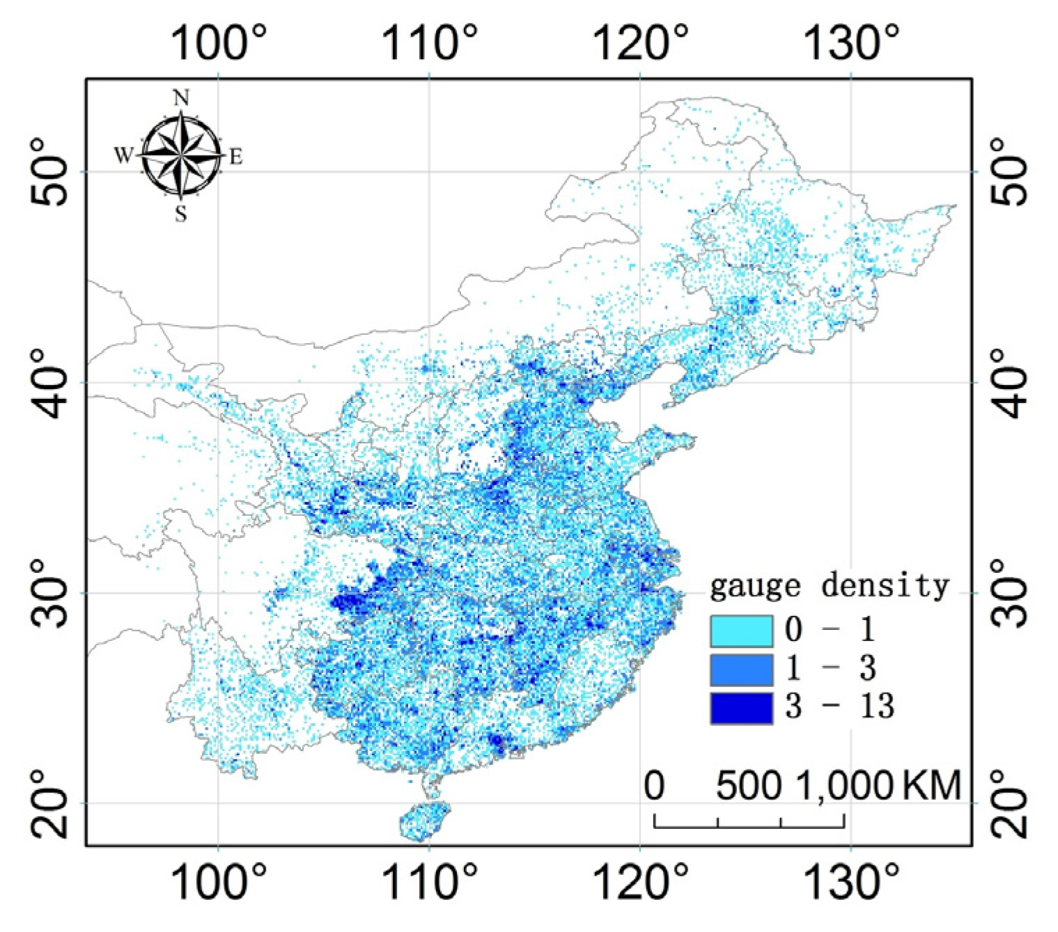
2.2.1. Rain Gauge Data

In this study, the hourly rain gauge observations from more than 30,000 automatic weather stations (AWSs) located in mainland China were used as the reference data. These observations undergo serious quality control including analysis of extremes, contiguous values, and spatial consistency checking. The quality-controlled data is then interpolated onto regular grid dataset with 0.1° using a modified climatology-based OI interpolation algorithm [26]. Currently, this dataset has been successfully used to validate high-resolution SPDs and generate multi-source precipitation datasets over mainland China [27]. In this study, only the grids with at least one rain gauge were selected to evaluate the IMERG in order to keep the reliability of these reference data. The spatial distribution of the rain gauges is heterogeneous (as showed by Figure 1). More than 60% of the rain gauges are located over the south part of the study area, whereas there are sparse rain gauges over the north part.

2.2.2. IMERG Satellite Precipitation Dataset

IMERG is generated by an algorithm based on the studies of producing the Tropical Rainfall Measuring Mission (TRMM) Multi-satellite Precipitation Analysis (TMPA) [8], CMORPH [10], and Precipitation Estimation from Remotely Sensed Information using Artificial Neural Networks-Cloud Classification System (termed as PERSIANN-CCS) [28], respectively. The main procedures of the algorithm used in IMERG include the following steps: (1) the precipitation estimates based on PMW observations from various satellites are inter-calibrated with the GPM Combined Instrument product; (2) the PMW precipitation datasets are propagated by the motion vectors derived from the infrared brightness temperatures; (3) the results of the second step are calibrated by Global Precipitation Climatology Centre precipitation datasets (termed as GPCC). It should be noted that IMERG has three runs for different applications (including Early, Late, and Final run). The Early run and Late run are about 4 h and 12 h after the observation time, which are suitable for time-sensitive applications (such as prediction of flash floods). The Final run is about two months after the observation time with GPCC adjustment to alleviate bias, which can be applied in research studies concerning climatology and ecology. In this study, we focus on considering the Final run IMERG with half-hour scale from April to October in 2014 (downloaded from https://storm-pps.gsfc.nasa.gov/storm/ (in which both of the calibrated and un-calibrated datasets are included)).

2.3. Method

This study focuses on evaluating and comparing the total bias and decomposed bias of IMERG before and after calibration by GPCC (termed as precipitationUncal and precipitationCal, respectively) over the eastern part of mainland China during the warm season. Additionally, the hit bias of IMERG is further decomposed according to rainfall intensity of the rain gauge measurements. The detailed steps of the evaluation process are as follows:
(1)
The rain gauge measurements and IMERG are pre-processed. First, the precipitationUncal and precipitationCal are summed up from half-hour to hourly scale. Second, the rain gauge measurements, precipitationUncal, and precipitationCal at same location and time are matched together.
(2)
The total biases of the precipitationUncal and precipitationCal are calculated according to the Equation (1):
bias = k = 1 n ( I k - O k ) / n
where Ik is the precipitation estimated by IMERG; Ok is the observation of rain gauge;
(3)
The bias calculated by Equation (1) is decomposed into three independent components including missed bias (rain areas which are incorrectly determined as no-rain areas by IMERG, termed as MB), false bias (no-rain areas which are incorrectly determined as rain areas by IMERG, termed as FB), and hit bias (the rain areas correctly determined by IMERG, but the precipitation intensity is inaccurately estimated, termed as HB) by Equations (2)–(4), respectively. It is obvious that the sum of the FB, MB, and HB is equal to the bias, but the magnitude of some components could exceed the total bias because the three components could cancel each other.
F B = f = 1 F ( I f ) / n
H B = h = 1 H ( O h ) / n
M B = m = 1 M ( I m - O m ) / n
where FB, HB, and MB are the false bias, hit bias, and missed bias, and F, H, and M are the number of false alarmed grids, hit grids, and missed detected grids, respectively. Oh, and Om are the rain gauge observation at hit grids and missed detected grids, respectively. In contrast, If, and Im are the precipitation estimated by IMERG at false alarmed grids and missed detected grids, respectively. Ok is the observation measured by rain gauge k, and n is the number of all grids over the study area.
(4)
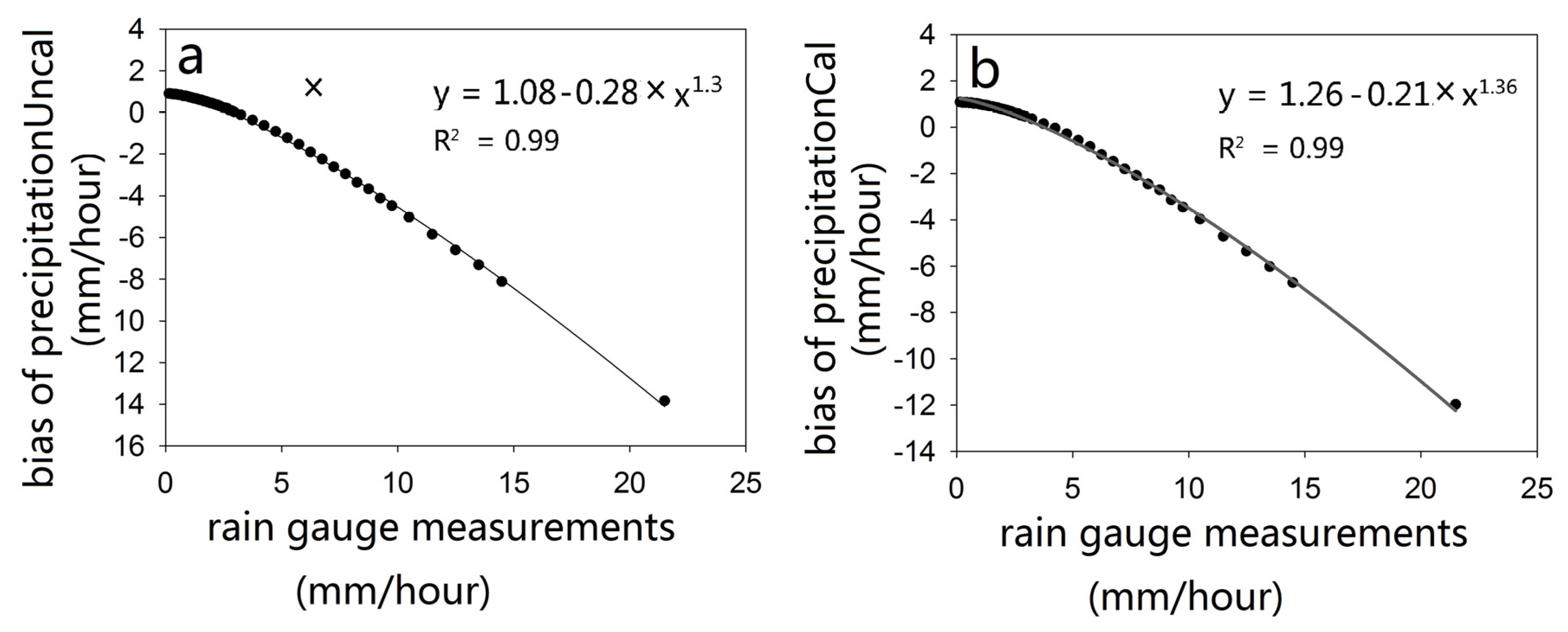
The HB of IMERG is further decomposed according to the precipitation intensity of the rain gauge measurements, with the aim of investigating whether any quantitative or qualitative relationships exist between them. To perform this analysis, all samples of hit bias are separated into 49 groups using the following thresholds: first, the samples with Rain gauge measurements values above 0 and no more than 3 mm/hour are separated into 30 groups with 0.1 mm/hour per step. Second, the samples with rain gauge measurements between 3 mm/hour and 10 mm/hour are separated into 14 groups for each 0.5 mm/hour step. Third, the samples with IMERG between 10 mm/hour and 15 mm/hour are separated into 5 groups at each 1 mm/hour step. Then the bias of each group is calculated according to the Equation (1).

3. Results

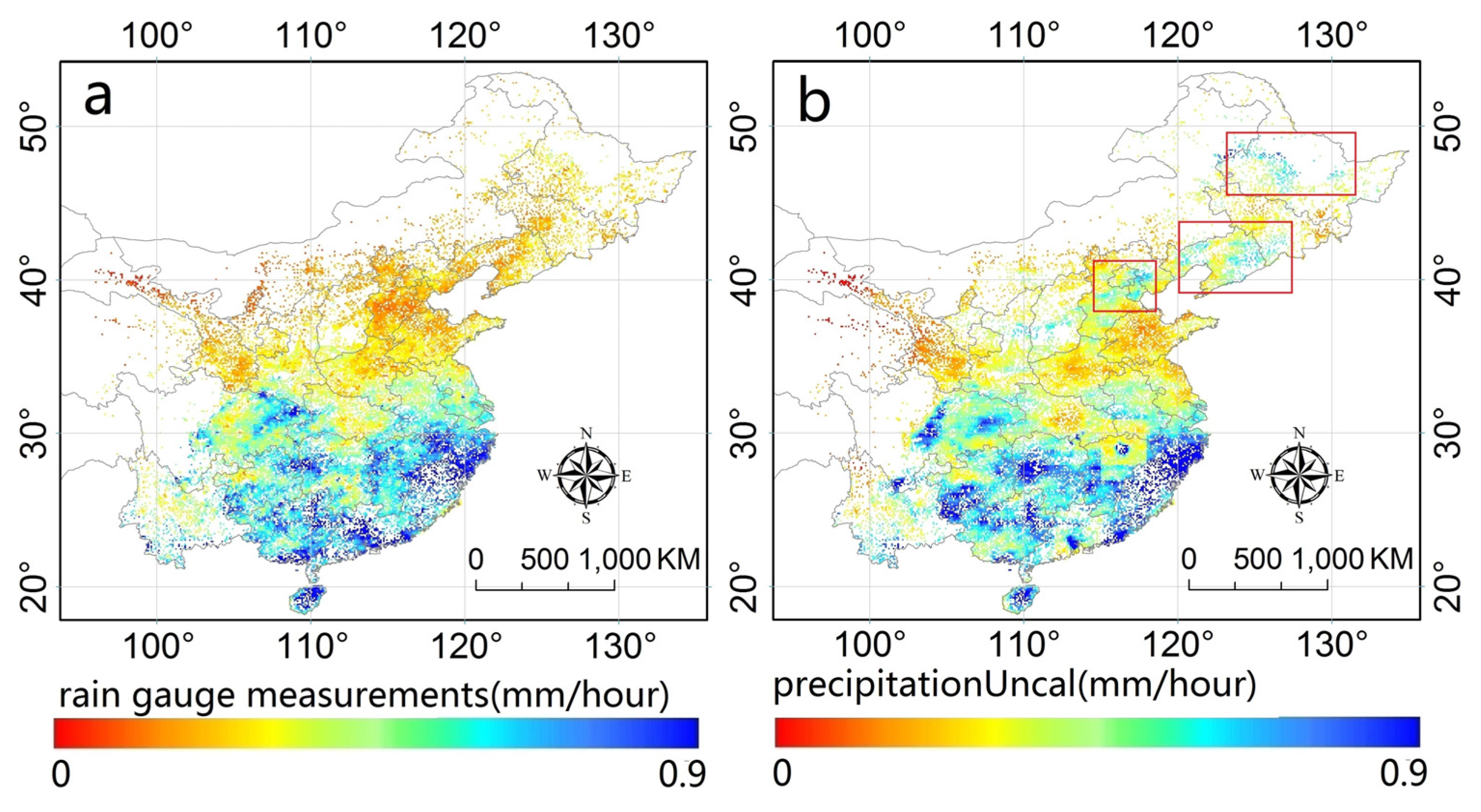
3.1. Spatial Pattern of the IMERG

In this study, we calculated the mean precipitation intensity of the gauge, precipitationUncal, and precipitationCal to analyze whether the IMERG could reflect the spatial pattern of the precipitation over the study area. Additionally, the values of the precipitationUncal and precipitationCal were compared grid by grid to investigate the influence of the calibration algorithm for different regions. As shown in Figure 2a, the spatial pattern of the precipitation over the study area presents an obvious regional characteristic whereby the precipitation increases from north to south. Both precipitationUncal and precipitationCal capture this characteristic relatively well (as shown in Figure 2b,c), but the former tends to overestimate the precipitation over the north part (as marked by red rectangles in Figure 2b). In contrast, the precipitationCal presents much lower precipitation than precipitationUncal over these regions, indicating that these errors in precipitationUncal could be effectively alleviated after the calibration process. Additionally, we compared the values of the precipitationUncal and precipitationCal grid by grid (as shown by Figure 2d), and the result indicates that the calibration algorithm used by IMERG tends to elevate the precipitationUncal over the north part but reduces it over the south part.
Figure 3 presents the scatter plots between the mean hourly rain gauge measurements and precipitationUncal and precipitationCal, respectively. The solid line shows the linear least squares relationship between the rain gauge measurements and the IMERG, and the dash line is the 1:1 line. Considering the precipitation presented obvious regional characteristics (as shown in Figure 2), this research was conducted by dividing the study area into a north part and south part with 36° N serving as the line of demarcation. It can be seen in Figure 3a that the precipitationUncal and rain gauge measurements did not present a very strong relationship over either the north (R2 = 0.43) or south part (R2 = 0.47), and that precipitationUncal showed better performance over the north part of mainland China than the south part. A notable characteristic of precipitationUncal is that it tends to underestimate the precipitation over the north part while it overestimates the precipitation over the south part. In contrast, precipitationCal shows much better performance than precipitationUncal with more than a 50% higher R2 and about 30%~40% lower root-mean-square-error (termed as RMSE). It should be noted that precipitationCal overestimates the precipitation over most of the southern part of mainland China, which is different from precipitationUncal.

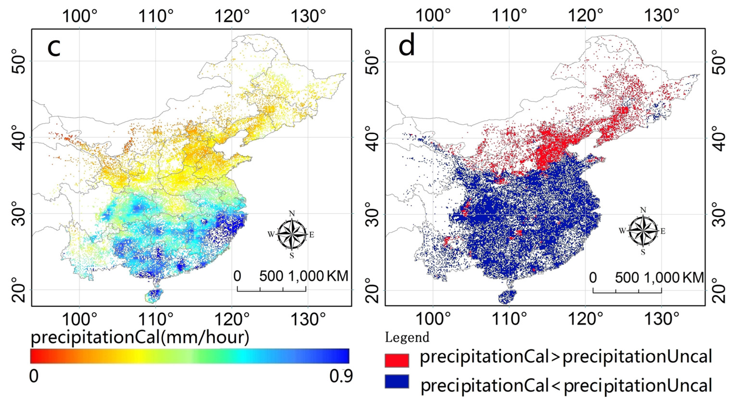
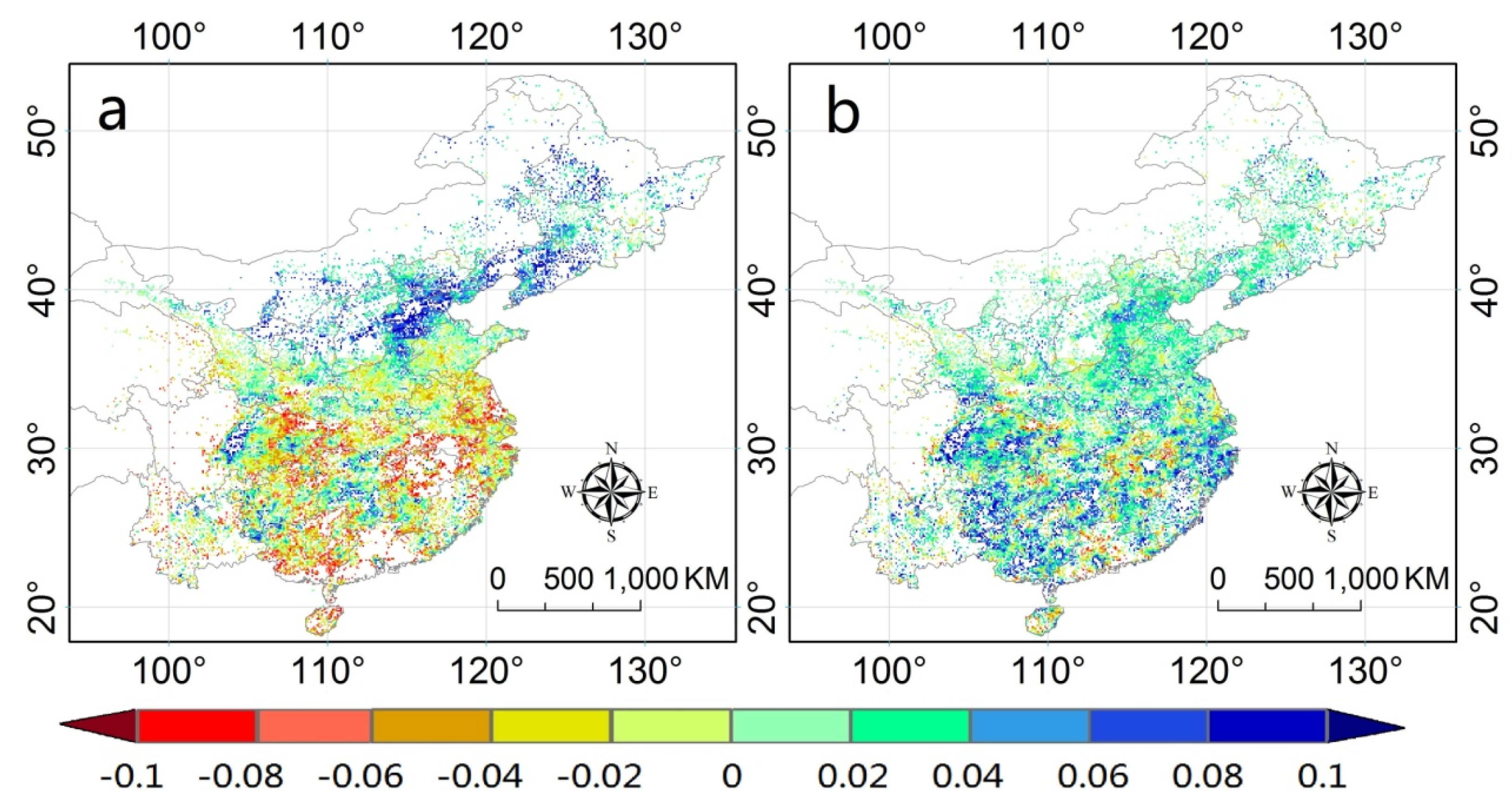
3.2. Bias Decomposition

The total bias of precipitationUncal and precipitationCal was calculated and decomposed into three independent components according to the methods illustrated in Section 2.3. The spatial patterns of the total bias contained in the two datasets are presented by Figure 4. It can be seen from Figure 4a that the total bias of precipitationUncal exhibited obvious regional characteristics, for example, it overestimates the precipitation in the north part while it underestimates precipitation over the south part of the study area. In contrast, the precipitationCal presented overestimations across most grids of the study areas (about 80%), but it showed less bias than precipitationUncal for the north part (Figure 4b).
Figure 5 shows the decomposed components of the total bias contained in precipitationUncal and precipitationCal. It can be inferred from this figure that the calibration algorithm used by IMERG brings different influences to the three decomposed components. The FB of precipitationUncal (Figure 5a) mainly ranges from 0.02 mm/hour to 0.04 mm/hour and presented smooth variation in space. However, we note the relatively high FB for the North China Plain where serious air pollution happens (about 35°~40° E, 112°~120° E, denoted by the red rectangle in Figure 5a), revealing potential evidence that the air pollution may be an important inducement of false bias. By visually comparing the FB of precipitationCal (Figure 5b) and precipitationUncal, it can be concluded that the calibration algorithm of IMERG could alleviate the FB over the North China Plain but enlarge the FB over the south part of the study area. Figure 5c,d illustrated the spatial pattern of the MB of precipitationUncal and precipitationCal. It should be pointed out that the calibrated algorithms used by IMERG could not correct the rain areas delineation, therefore, the MB of precipitationUncal and precipitationCal shared the same spatial pattern. Generally, it can be seen in these figures that the MB increases from north to south with the range between 0.01 and 0.15 mm/hour. The HB of precipitationUncal and precipitationCal is presented in Figure 5e,f, respectively. The precipitationUncal yielded positive HB over 51% of the grids which are mainly distributed over the north part of the study area, while this ratio increased to 82% for precipitationCal. Especially, the calibration algorithm of IMERG seriously enlarged the HB over some regions over the south part (denoted by red rectangles in Figure 5f).
Further analysis was performed to investigate the sources of the bias inherent in IMERG, with the aim of providing quantitative information which is indispensable for its application and possible correction. Table 1 presents the average amplitudes of the total errors and three decomposed components for the north part and south part of mainland China (with 36° N serving as the line of demarcation). It can be seen in this table that both PrecipitationUncal and PrecipitationCal overestimate the precipitation over the south part, but that the calibration algorithm could effectively account for the hit bias contained in PrecipitationUncal in this region. In the north part, the amplitude of the total bias contained in PrecipitationCal is smaller than PrecipitationUncal mainly because the hit bias changed from negative to positive after the calibration process.
The HB of the precipitationUncal and precipitationCal was further decomposed according to the precipitation intensity measured by rain gauges (Figure 6). We found that both precipitationUncal and precipitationCal tend to overestimate the light precipitation while underestimating the heavy precipitation. Additionally, the relationship between the rain gauge measurements and the HB could be described by a three parameters power function with the determination of coefficient above 0.99, which provided useful information to alleviate the HB of IMERG.

4. Discussion

Although previous studies [14,29,30] have revealed that the IMERG showed more notable progress than existing SPDS, it can be inferred from the results of this study that both precipitationUncal and precipitationCal present notable bias over some regions of the study area. In our opinion, two reasons may be responsible for the uncertainty contained in IMERG: (1) Retrieving precipitation from PMW observations using Goddard Profiling Algorithm (GPROF) is the key process to produce IMERG, and the performance of GPROF largely relies upon the quality of the database composed by the pairs between the hydrometeor profile and PMW brightness temperature [31]. The DPR loaded on the GPM Core Observatory is designed to retrieve a high-quality hydrometeor profile which is synchronous with the PWM brightness temperature observed by the GMI. However, the hydrometeor profile acquired by the DPR loaded on the GPM Core Observatory is not used in the first version of IMERG because the number of DPR observations is not enough to finalize this database. Currently, the observations from national oceanic and atmospheric administration (termed as NOAA) National Mosaic and Multi-Sensor quantitative precipitation estimation (termed as QPE) radar are used as substitutes over land and divided into ten classes according to the land surface characteristics, but they could not provide comprehensive characteristics for hydrometeor profiles all over the world, which may lead to uncertainty associated with IMERG; (2) Michaelides et al. [32] revealed that the retrieval algorithm of SPD is usually optimized for particular regions, which could make the SPD less adapted for other regions. To our knowledge, there has been no evidence about the adjustment of the IMERG for mainland China until now. This may be one possible reason for the uncertainty of the IMERG over this area.
The results of this research also reveal a shortcoming of the calibration algorithm used by IMERG which calibrates the precipitation retrieved from satellite observations (termed as SP) by multiplying the ratio of the SP and the satellite-gauge merged precipitation datasets (termed as SG) at a monthly scale [8,9]. The advantage of this algorithm is that it creates a correction coefficient for each grid and for each month, which are beneficial for reducing the regional and seasonal bias contained in SPD. However, it does not change the rain gauge rain areas delineation, so the missed precipitation and false precipitation which are only contained in high resolution SPDs could not be alleviated [33]. This limitation may lead to various influences on the performance of this algorithm. First, for the missed detected precipitation, this algorithm could not influence the missed bias because the value of IMERG over the missed detected grids is zero. For the false alarmed grids, if the SG/MG ratio is smaller or equal to 1, the false bias will be alleviated or kept unchanged, but if the SG/MG ratio is above 1, the multiplication of this ratio and the un-calibrated IMERG will enlarge the magnitude of the false alarmed precipitation. For the grid in which false alarmed precipitation is serious and the SG/MG ratio is above 1, the enlarged false alarmed precipitation may offset the improvement of the hit bias, leading to an even poorer performance of the calibrated IMERG than the un-calibrated IMERG. It can be inferred from Figure 4 that the calibration algorithm tends to elevate the values of the precipitationUncal over the south part of the study area, leading to the deterioration of the false bias. Therefore, we strongly suggest that there is a significant need to pay more attention to eliminate the false alarmed and missed detected precipitation in the IMERG before its application. However, it should be clearly pointed out that this is a preliminary conclusion about the characteristics and sources of the errors contained in the IMERG over mainland China because this dataset was retrieved using the at-launch algorithm. More investigations will be conducted for the future versions of IMERG.

5. Conclusions

In this study, the bias of the hourly IMERG before and after calibration with GPCC was evaluated and compared with each other with supporting rain gauge data for eastern mainland China. Then, the total bias was decomposed into three independent components including false bias, missed bias, and hit bias to investigate the characteristics and the sources of the biases. Additionally, the hit bias was further decomposed according to the precipitation intensity. Several conclusions can be drawn from the results of this study:
(1)
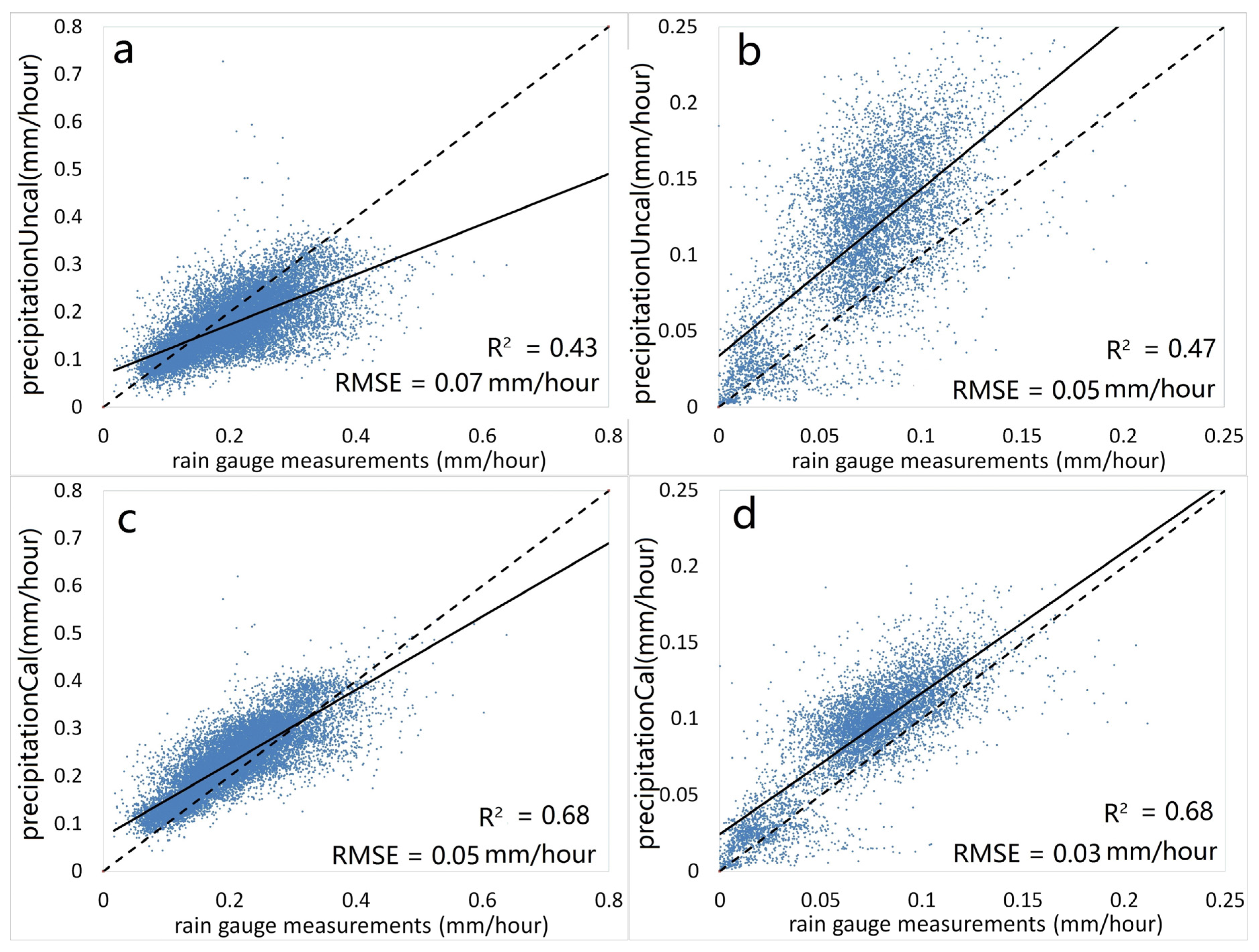
Both precipitationUncal and precipitationCal could capture the spatial pattern of the precipitation over the study, but the former could better estimate the precipitation volume than the latter.
(2)
The calibration algorithm used by IMERG could significantly reduce the hit bias over the south regions, but it exaggerated the false bias over the south part. Additionally, this algorithm could not alleviate the missed bias of IMERG, which is largely responsible for the bias over the south part of the IMERG.
(3)
The false bias and hit bias were responsible for a large part of the total bias of both precipitationUncal and precipitationCal. Therefore, considerations concerning how to retrieve more accurate rain areas delineation using satellite observations deserve more attention in order to better apply and improve the application of IMERG in future work.
(4)
There was a strong non-linear relationship between the hit bias of IMERG and the rainfall intensity measured by rain gauges, which could be beneficial for the further correction of this new satellite precipitation dataset.

Acknowledgments

This work was funded by National Science Foundation of China Major research program (91437214) and National Natural Science Foundation of China (Grant No. 8960327).

Author Contributions

Shiguang Xu and Yan Shen conceived and designed the experiments and analyze the data; Shiguang Xu and Zhe Du performed the experiments; Yan Shen contributed the rain gauge measurements; Shiguang Xu wrote the paper.

Conflicts of Interest

The authors declare no conflict of interest.

References

  1. Yong, B.; Liu, D.; Gourley, J.J.; Tian, Y.; Huffman, G.J.; Ren, L.; Hong, Y. Global view of real-time TRMM multisatellite precipitation analysis: Implications for its successor global precipitation measurement mission. Bull. Am. Meteorol. Soc. 2015, 96, 283–296. [Google Scholar] [CrossRef]
  2. Xu, S.-G.; Niu, Z.; Shen, Y. Understanding the dependence of the uncertainty in a satellite precipitation data set on the underlying surface and a correction method based on geographically weighted regression. Int. J. Remote Sens. 2014, 35, 6508–6521. [Google Scholar] [CrossRef]
  3. Habib, E.; Henschke, A.; Adler, R.F. Evaluation of tmpa satellite-based research and real-time rainfall estimates during six tropical-related heavy rainfall events over louisiana, USA. Atmos. Res. 2009, 94, 373–388. [Google Scholar] [CrossRef]
  4. Haile, A.T.; Yan, F.; Habib, E. Accuracy of the cmorph satellite-rainfall product over lake tana basin in eastern africa. Atmos. Res. 2014, 163, 177–187. [Google Scholar] [CrossRef]
  5. Grody, N.C. Classification of snow cover and precipitation using the special sensor microwave imager. J. Geophys. Res. Atmos. 1991, 96, 7423–7435. [Google Scholar] [CrossRef]
  6. Ferraro, R.R.; Grody, N.C.; Marks, G.F. Effects of surface conditions on rain identification using the DMSP-SSM/I. Remote Sens. Rev. 1994, 11, 195–209. [Google Scholar] [CrossRef]
  7. Gebregiorgis, A.S.; Hossain, F. How well can we estimate error variance of satellite precipitation data around the world? Atmos. Res. 2015, 154, 39–59. [Google Scholar] [CrossRef]
  8. Huffman, G.J.; Adler, R.F.; Arkin, P.; Chang, A.; Ferraro, R.; Gruber, A.; Janowiak, J.; McNab, A.; Rudolf, B.; Schneider, U. The global precipitation climatology project (gpcp) combined precipitation dataset. Bull. Am. Meteorol. Soc. 1997, 78, 5–20. [Google Scholar] [CrossRef]
  9. Huffman, G.J.; Adler, R.F.; Bolvin, D.T.; Gu, G.J.; Nelkin, E.J.; Bowman, K.P.; Hong, Y.; Stocker, E.F.; Wolff, D.B. The TRMM multisatellite precipitation analysis (TMPA): Quasi-global, multiyear, combined-sensor precipitation estimates at fine scales. J. Hydrometeorol. 2007, 8, 38–55. [Google Scholar] [CrossRef]
  10. Joyce, R.J.; Janowiak, J.E.; Arkin, P.A.; Xie, P.P. Cmorph: A method that produces global precipitation estimates from passive microwave and infrared data at high spatial and temporal resolution. J. Hydrometeorol. 2004, 5, 487–503. [Google Scholar] [CrossRef]
  11. Huffman, G.J. The Global Precipitation Measurement (GPM) Mission: An Overview. Available online: https://ntrs.nasa.gov/search.jsp?R=20060026287 (accessed on 12 December 2016).
  12. Tapiador, F.J.; Turk, F.J.; Petersen, W.; Hou, A.Y.; García-Ortega, E.; Machado, L.A.T.; Angelis, C.F.; Salio, P.; Kidd, C.; Huffman, G.J. Global precipitation measurement: Methods, datasets and applications. Atmos. Res. 2012, 104–105, 70–97. [Google Scholar] [CrossRef]
  13. Hou, A.Y.; Kakar, R.K.; Neeck, S.; Azarbarzin, A.A.; Kummerow, C.D.; Kojima, M.; Oki, R.; Nakamura, K.; Iguchi, T. The global precipitation measurement (GPM) mission. Bull. Am. Meteorol. Soc. 2014, 95, 701–722. [Google Scholar] [CrossRef]
  14. Prakash, S.; Mitra, A.K.; Aghakouchak, A.; Liu, Z.; Norouzi, H.; Pai, D.S. A preliminary assessment of GPM-based multi-satellite precipitation estimates over a monsoon dominated region. J. Hydrol. 2016. [Google Scholar] [CrossRef]
  15. Guo, H.; Chen, S.; Bao, A.; Behrangi, A.; Hong, Y.; Ndayisaba, F.; Hu, J.; Stepanian, P.M. Early assessment of integrated multi-satellite retrievals for global precipitation measurement over China. Atmos. Res. 2016, 176–177, 121–133. [Google Scholar] [CrossRef]
  16. Tang, G.; Ma, Y.; Long, D.; Zhong, L.; Hong, Y. Evaluation of GPM day-1 imerg and TMPA version-7 legacy products over mainland China at multiple spatiotemporal scales. J. Hydrol. 2015, 533, 152–167. [Google Scholar] [CrossRef]
  17. Shen, Y.; Xiong, A.Y.; Wang, Y.; Xie, P.P. Performance of high-resolution satellite precipitation products over China. J. Geophys. Res. Atmos. 2010, 115. [Google Scholar] [CrossRef]
  18. Xie, P.P.; Xiong, A.Y. A conceptual model for constructing high-resolution gauge-satellite merged precipitation analyses. J. Geophys. Res. Atmos. 2011, 116. [Google Scholar] [CrossRef]
  19. Salio, P.; Hobouchian, M.P.; Skabar, Y.G.; Vila, D. Evaluation of high-resolution satellite precipitation estimates over southern south america using a dense rain gauge network. Atmos. Res. 2015, 163, 146–161. [Google Scholar] [CrossRef]
  20. Maggioni, V.; Meyers, P.C.; Robinson, M.D. A review of merged high-resolution satellite precipitation product accuracy during the tropical rainfall measuring mission (TRMM) era. J. Hydrometeorol. 2016, 17. [Google Scholar] [CrossRef]
  21. Oliveira, R.A.J.; Braga, R.C.; Vila, D.A.; Morales, C.A. Evaluation of GPROF-SSMI/S rainfall estimates over land during the brazilian chuva-vale campaign. Atmos. Res. 2014, 163, 102–116. [Google Scholar] [CrossRef]
  22. Oliveira, R.; Maggioni, V.; Vila, D.; Morales, C. Characteristics and diurnal cycle of GPM rainfall estimates over the central amazon region. Remote Sens. 2016, 8, 544. [Google Scholar] [CrossRef]
  23. Tian, Y.; Peters-Lidard, C.D.; Eylander, J.B.; Joyce, R.J.; Huffman, G.J.; Adler, R.F.; Hsu, K.L.; Turk, F.J.; Garcia, M.; Zeng, J. Component analysis of errors in satellite-based precipitation estimates. J. Geophys. Res. Atmos. 2009, 114. [Google Scholar] [CrossRef]
  24. Tang, L.; Tian, Y.; Yan, F.; Habib, E. An improved procedure for the validation of satellite-based precipitation estimates. Atmos. Res. 2015, 163, 61–73. [Google Scholar] [CrossRef]
  25. Gebregiorgis, A.S.; Tian, Y.; Peters-Lidard, C.D.; Hossain, F. Tracing hydrologic model simulation error as a function of satellite rainfall estimation bias components and land use and land cover conditions. Water Resour. Res. 2012, 48, W11509. [Google Scholar] [CrossRef]
  26. Xie, P.; Yatagai, A.; Chen, M.; Hayasaka, T.; Fukushima, Y.; Liu, C.; Yang, S. A gauge-based analysis of daily precipitation over east Asia. J. Hydrometeorol. 2007, 8, 607. [Google Scholar] [CrossRef]
  27. Shen, Y.; Zhao, P.; Pan, Y.; Yu, J. A high spatiotemporal gauge-satellite merged precipitation analysis over China. J. Geophys. Res. Atmos. 2014, 119, 3063–3075. [Google Scholar] [CrossRef]
  28. Hsu, K.L.; Gao, X.G.; Sorooshian, S.; Gupta, H.V. Precipitation estimation from remotely sensed information using artificial neural networks. J. Appl. Meteorol. 1997, 36, 1176–1190. [Google Scholar] [CrossRef]
  29. Prakash, S.; Mitra, A.K.; Pai, D.S.; Aghakouchak, A. From TRMM to GPM: How well can heavy rainfall be detected from space? Adv. Water Res. 2015, 88, 1–7. [Google Scholar] [CrossRef]
  30. Gaona, M.F.R.; Overeem, A.; Leijnse, H.; Uijlenhoet, R. First-year evaluation of GPM-rainfall over the Netherlands: Imerg day-1 final run (v03d). J. Hydrometeorol. 2016, 17, 2799–2814. [Google Scholar] [CrossRef]
  31. Kummerow, C.; Hong, Y.; Olson, W.S.; Yang, S.; Adler, R.F.; McCollum, J.; Ferraro, R.; Petty, G.; Shin, D.B.; Wilheit, T.T. The evolution of the goddard profiling algorithm (GPROF) for rainfall estimation from passive microwave sensors. J. Appl. Meteorol. 2001, 40, 1801–1820. [Google Scholar] [CrossRef]
  32. Michaelides, S.; Levizzani, V.; Anagnostou, E.; Bauer, P.; Kasparis, T.; Lane, J.E. Precipitation: Measurement, remote sensing, climatology and modeling. Atmos. Res. 2009, 94, 512–533. [Google Scholar] [CrossRef]
  33. Yong, B.; Ren, L.; Hong, Y.; Gourley, J.J.; Tian, Y.; Huffman, G.J.; Chen, X.; Wang, W.; Wen, Y. First evaluation of the climatological calibration algorithm in the real-time tmpa precipitation estimates over two basins at high and low latitudes. Water Resour. Res. 2013, 49, 2461–2472. [Google Scholar] [CrossRef]
Figure 1. The study area and the locations of the rain gauges during the warm season.
Atmosphere 07 00161 g001
Figure 2. The spatial pattern of the hourly precipitation intensity measured by (a) rain gauge measurements; (b) un-calibrated Integrated Multi-satellite Retrievals for Global Precipitation Measurement (IMERG) (termed as precipitationUncal); (c) calibrated IMERG (termed as precipitationCal); (d) the comparison result of precipitationUncal and precipitationCal for each grid during April~October in 2014.
Atmosphere 07 00161 g002aAtmosphere 07 00161 g002b
Figure 3. The scatter plots between the mean hourly rain gauge measurements and (a) IMERG before calibration (termed as precipitationUncal) over the north part of mainland China; (b) precipitationUncal over the south part of mainland China; (c) IMERG after calibration (termed as precipitationCal) over the north part of mainland China; (d) precipitationCal over the south part of mainland China.
Atmosphere 07 00161 g003
Figure 4. The spatial pattern of the bias contained in (a) un-calibrated IMERG and (b) calibrated IMERG.
Atmosphere 07 00161 g004
Figure 5. The spatial pattern of the decomposed bias of un-calibrated IMERG and calibrated IMERG. (a) the false bias of un-calibrated IMERG; (b) the false bias of calibrated IMERG; (c) the missed bias of un-calibrated IMERG; (d) the missed bias of calibrated IMERG; (e) the hit bias of un-calibrated IMERG; (f) the hit bias of calibrated IMERG.
Atmosphere 07 00161 g005
Figure 6. The scatter plots between the rain gauge measurements and the bias (bias) of hit bias contained in (a) un-calibrated IMERG (termed as precipitationUncal) and (b) calibrated IMERG (termed as precipitationCal).
Atmosphere 07 00161 g006
Table 1. Averaged error components of IMERG before and after calibration (termed as precipitationUncal and precipitationCal) as percentages of total precipitation measured by rain gauges for north and south parts of mainland China
RegionDatasetTotal BiasFalse BiasMissed BiasHit Bias
South partPrecipitationUncal58.2%38.6%−20.8%40.4%
PrecipitationCal27.7%32.5%−20.8%16.0%
North partPrecipitationUncal−13.6%17.0%−23.8%−6.8%
PrecipitationCal12.9%23%−23.8%13.7%

