Future Streamflow Projections in a Semi-Arid Mountain Basin Using Machine Learning and CMIP6 Climate Scenarios: The Case of the Zat River (Morocco)

Abstract

Understanding how climate change may alter river discharge in semi-arid regions is essential for sustainable water-resource management. This study assesses future streamflow in the Zat River Basin (High Atlas Mountains, Morocco) using a hybrid framework that combines machine-learning rainfall–runoff modeling, CMIP6 multi-model climate forcing, monthly quantile-mapping post-processing of simulated discharge, and an exploratory temperature-sensitivity assessment. Monthly hydroclimatic observations of precipitation, air temperature, reference evapotranspiration, and discharge were compiled from February 1962 to August 2024. The period 1962–2005 was used for model development, the 2006–2014 window for chronological validation, and the more recent observations for supplementary evaluation of climate-driven simulations. Four algorithms were compared: Gradient Boosting Regressor (GBR), Histogram-based Gradient Boosting Regressor (HGBR), Random Forest (RF), and Multi-Layer Perceptron (MLP). Performance was assessed using NSE, KGE, RMSE, MAE, and R². GBR provided the best validation performance (NSE = 0.71, KGE = 0.80, and R² = 0.72). The selected model was then forced with CMIP6 projections under SSP2-4.5 and SSP5-8.5 to simulate streamflow to 2100. Quantile mapping was applied to the simulated discharge, rather than separately to precipitation, temperature, and reference evapotranspiration. The multi-model ensemble indicates a persistent drying tendency: relative to the historical baseline and without an additional temperature-sensitivity adjustment, mean annual discharge is projected to decline by approximately 12.1% under SSP2-4.5 and 27.3% under SSP5-8.5 by 2081–2100. Under an exploratory sensitivity case using a runoff-temperature-sensitivity coefficient of 0.04 °C⁻¹, the projected declines increase to approximately 23.3% and 44.1%, respectively. Episodic high-flow events nevertheless remain possible, suggesting a shift toward lower mean flows combined with persistent hydrological extremes.

1. Introduction

Mountainous semi-arid basins are among the most climate-sensitive hydrological systems globally, owing to their dependence on snowpack formation, snowmelt timing, steep topographic gradients, and highly seasonal precipitation regimes [1,2]. In such environments, streamflow generation is controlled by complex interactions between orographic precipitation, snow accumulation and melt, evapotranspiration, soil moisture dynamics, fractured geological formations, and delayed subsurface contributions. These processes often produce strong non-linearities, threshold responses, and hydrological memory effects, which make runoff simulation particularly challenging under both historical and future climate conditions.

The High Atlas Mountains in Morocco form one of the most important water towers in the country, sustaining nearly 70% of surface water resources in the Tensift and Oum-Er-Rbia basins [3,4]. Recent climatic trends show marked warming, intensified drought frequency, declining snow cover, and substantial contraction of mountain cryosphere resources [5,6]. These changes directly affect the seasonal distribution of runoff, particularly by reducing snow accumulation, advancing snowmelt timing, and weakening spring baseflow contributions. Consequently, the reliability of water supplies for downstream agricultural, domestic, and ecological needs is increasingly threatened.

In parallel, Morocco is facing a structural water scarcity crisis, aggravated by a succession of extreme droughts, increasing irrigation demand, groundwater overexploitation, and rapid urban expansion [7]. The Zat Basin, a tributary of the Tensift system, is emblematic of these tensions: it supplies essential seasonal inflows to the Haouz plain, supports rural livelihoods, and contributes to downstream ecological flows [8]. Yet its hydrological balance is highly sensitive to climate-induced perturbations, especially because runoff depends on a limited number of precipitation events, seasonal snowmelt, and highly variable antecedent moisture conditions.

Climate projections for North Africa consistently indicate future warming of +2 °C to +6 °C and a 10–30% decrease in precipitation by the end of the twenty-first century [9,10,11]. These developments are expected to produce nonlinear hydrological impacts due to amplified evapotranspiration, reduced soil moisture, decreased snow accumulation, earlier snowmelt, and altered runoff generation processes [12,13]. For semi-arid mountain basins, even moderate changes in precipitation and temperature may lead to disproportionate reductions in streamflow, because the hydrological response is strongly influenced by threshold effects, storage depletion, and catchment memory.

Climate-change impact assessments have traditionally relied on conceptual and physically based rainfall–runoff models. Physically based models provide explicit process representation and are constrained by water and energy balances, but they generally require detailed spatial data, substantial parameterization, and reliable information on snow, soils, and groundwater exchanges. Conceptual models are more parsimonious, yet their calibrated parameters may not remain transferable under strongly non-stationary conditions. Machine-learning models offer a complementary approach because they can capture nonlinear predictor–response relationships and hydrological memory from available observations; however, they do not explicitly represent all physical processes and may have limited extrapolation capacity outside the historical training domain. The present study therefore does not claim that machine learning replaces process-based modeling; rather, it evaluates a data-driven alternative for a heterogeneous, data-constrained High Atlas basin and explicitly discusses its assumptions and limitations [14,15,16,17].

Recent advances in Artificial Intelligence (AI) and machine learning offer new capabilities for simulating rainfall-runoff dynamics without assuming rigid parametric structures [16,18,19,20]. Machine-learning methods, including Artificial Neural Networks (ANNs), Support Vector Regression (SVR), Random Forest (RF), Gradient Boosting Regression (GBR), Extreme Gradient Boosting (XGBoost), and deep learning approaches such as Long Short-Term Memory networks (LSTM), have been increasingly applied to streamflow simulation and forecasting. Their main advantage lies in their ability to capture complex and nonlinear relationships between precipitation, temperature, evapotranspiration, antecedent wetness conditions, snow-related processes, and discharge response.

Several studies have demonstrated the strong potential of machine learning and deep learning for streamflow simulation. Kratzert et al. [18] showed that LSTM networks can effectively simulate rainfall-runoff processes and learn long-term dependencies that are essential for representing catchment storage and snow-influenced hydrological behavior. In a subsequent large-sample study, Kratzert et al. [21] demonstrated that regional LSTM models trained over hundreds of catchments can learn transferable hydrological behavior and outperform several traditional hydrological modeling benchmarks. These findings indicate that data-driven models are not only useful for short-term forecasting but can also provide robust representations of catchment memory, seasonal storage, and delayed runoff response.

Beyond LSTM models, tree-based ensemble methods such as Random Forest, Gradient Boosting, and XGBoost have also shown strong performance in hydrological prediction because they can handle nonlinear interactions, variable importance ranking, and complex predictor–response relationships. Comparative studies in streamflow prediction have reported that advanced machine-learning algorithms can improve predictive accuracy relative to classical statistical approaches, particularly when hydroclimatic predictors and antecedent conditions are properly included [22,23]. These methods are especially relevant for semi-arid basins where runoff is controlled by intermittent rainfall, strong evapotranspiration demand, and threshold-driven hydrological responses.

In Morocco and similar semi-arid Mediterranean environments, recent studies have confirmed the relevance of machine learning for streamflow modeling. For example, Nifa et al. [24] applied LSTM networks to daily streamflow prediction in the semi-arid Ait Ouchene watershed of the Oum Er-Rbia Basin and showed that model performance improved substantially when lagged hydroclimatic inputs and feature selection were considered. Such results highlight the importance of antecedent precipitation, temperature, snow-related information, and catchment memory in Moroccan mountain hydrology. Nevertheless, most existing applications have focused on short-term or daily streamflow forecasting, while fewer studies have addressed long-term monthly streamflow simulation under climate-change scenarios in snow-influenced High Atlas basins.

Although the general combination of machine learning and climate scenarios is not unprecedented, important context-specific gaps remain. First, applications to semi-arid, snow-influenced High Atlas basins are still limited compared with those in temperate and humid regions. Second, few studies have integrated a hydroclimatic record extending for more than six decades, reference evapotranspiration, hydrologically informed feature engineering, chronological hold-out assessment, and a sixteen-member CMIP6 ensemble within a single monthly streamflow framework. Third, the Zat Basin remains poorly documented despite its strategic contribution to the Tensift system and its pronounced climatic heterogeneity. The contribution of this study therefore lies primarily in adapting and evaluating this integrated framework for a basin characterized by a strong elevation gradient, Mediterranean-continental influences, orographic precipitation, seasonal snow, and marked hydrological memory.

Accordingly, this study develops and evaluates an AI-based rainfall–runoff framework for historical and future monthly streamflow simulation in the Zat Basin. Tree-based ensemble methods and a neural-network model are compared using long-term monthly precipitation, temperature, reference evapotranspiration, and discharge observations. The selected model is then forced with CMIP6-derived climate series under SSP2-4.5 and SSP5-8.5, and the simulated discharge is post-processed using monthly quantile mapping. An additional temperature-sensitivity term is examined only as an exploratory sensitivity analysis. The objectives are to quantify potential streamflow changes to 2100, characterize ensemble uncertainty, and provide information relevant to climate-resilient water-resource planning in a semi-arid, snow-influenced High Atlas basin.

2. Study Area and Data

2.1. Geographical and Climatic Context

The Zat River Basin, with elevations ranging from approximately 900 to 4400 m above sea level, drains part of the northern High Atlas before joining the Tensift River east of Marrakech. It exhibits a pronounced altitudinal climatic gradient shaped by Mediterranean-continental influences, orographic uplift, and snow-dominated winter conditions [6,25].

This topographic gradient exerts fundamental control on climatic heterogeneity, hydrological processes, and surface water–groundwater interactions.

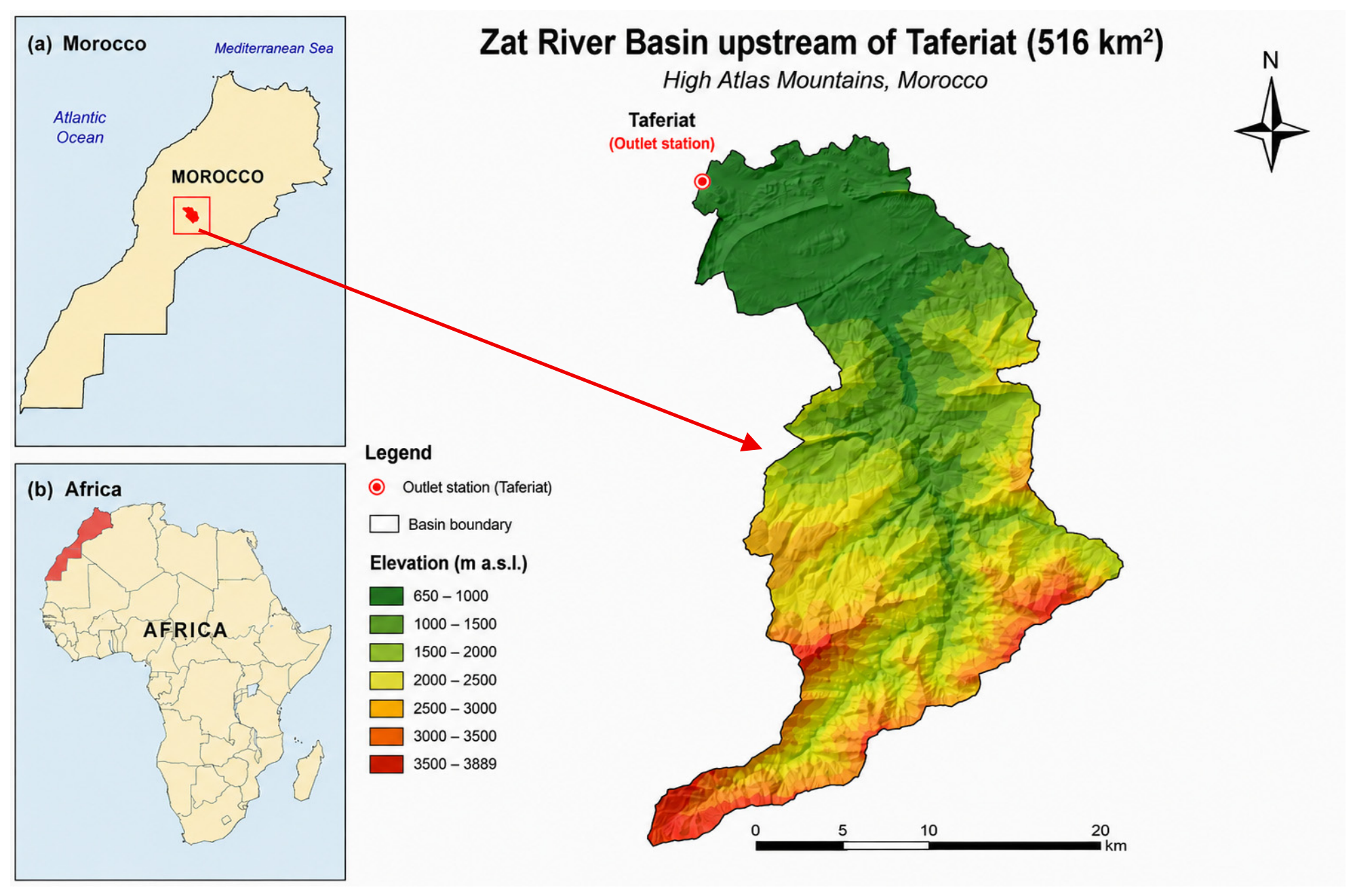
Figure 1 shows the location of the Zat River Basin on the northern flank of the High Atlas Mountains. The Taferiat gauging station defines the hydrological outlet of a catchment of approximately 516 km². The basin extends from elevations exceeding 4000 m upstream to about 900 m downstream; this steep morphology and strong altitudinal contrast contribute to marked hydrological seasonality and snow influence.

The basin has a Mediterranean climate with a semi-arid tendency that is strongly modulated by elevation. In the upper basin, cold winter conditions and snowfall generate a seasonal snowpack that contributes to spring and early-summer runoff. At mid-elevations, precipitation is highly variable and occurs mainly from November to April in association with North Atlantic disturbances. The lower basin has a pronounced dry season from May to September, when temperatures can exceed 40 °C. These climatic contrasts produce marked flow seasonality, with low flows generally occurring from July to September and occasional flash floods generated by convective storms.

Several studies have shown clear evidence of climate-change impacts in the High Atlas, including declining snowfall, rising temperature, and increasing interannual variability of precipitation [1,6]. These changes directly threaten the hydrological functioning of basins such as the Zat, which relies on the delicate balance between rainfall, snow accumulation, and snowmelt.

2.2. Hydrometeorological Dynamics of the Zat Basin

The hydrological functioning of the Zat Basin is governed by snow processes, orographic precipitation, ephemeral tributaries, and soil–vegetation interactions typical of semi-arid mountain environments. Mean annual precipitation increases from less than 250 mm downstream to more than 520 mm in the upper basin, consistent with gradients reported for other High Atlas catchments [8]. Winter precipitation frequently falls as snow above approximately 2600–2800 m. The seasonal snowpack acts as a natural reservoir and contributes substantially to spring runoff during periods of limited summer rainfall.

Temperature plays a critical role in modulating snowmelt timing, evapotranspiration losses, and soil-water availability. Observed records indicate a warming trend of +1.2 °C since the 1970s, consistent with broader regional trends in North Africa [10,11]. This warming accelerates snowmelt, reduces snow accumulation, and enhances evapotranspiration, leading to reduced spring flows and earlier recession of the hydrograph.

Geological and geomorphological features, particularly fractured bedrock and permeable alluvial formations, also contribute to subsurface storage and surface water–groundwater exchanges. These processes introduce time lags and non-linearities into the runoff response. Conceptual and lumped models can represent some of these dynamics, but their calibration may be challenging when observations of snow, soil moisture, and groundwater exchanges are limited. This context motivates the evaluation of machine-learning models as a complementary modeling approach rather than as a substitute for process-based models. The principal hydrometeorological characteristics of the Zat Basin over 1962–2024 are summarized in

Table 1. Summary of hydrometeorological characteristics for 1962–2024.

Variable	Mean	Min	Max	Trend (per Decade)	Notes
Precipitation (mm/year)	410	185	920	−2.3%	Strongly altitudinal gradient
Temperature (°C)	16.8	3.5	38	+0.32 °C	Significant warming trend
ET0 (mm/year)	1360	980	1640	+1.9%	Increasing due to warming
Discharge (m3/s)	2.31	0.01	280	−4%	Declining due to decreased snow contribution

.

2.3. Historical Hydrometeorological Data

Monthly precipitation (P), mean air temperature (T), reference evapotranspiration (ET₀), and discharge (Q) at the basin outlet were compiled from February 1962 to August 2024. The primary discharge data were obtained from the Tensift Hydraulic Bassin Agency (ABHT) monitoring network. The period 1962–2005 was used for model calibration, whereas 2006–2014 was retained for independent validation. Observations available after 2014 were not used to fit the validation metrics; they were used to extend the historical characterization and, where common dates were available, to provide a supplementary assessment of climate-driven simulations over the recent period.

After quality control, gap filling, and temporal aggregation, the dataset comprised:

• Monthly basin-average precipitation (P_mm);
• Monthly mean air temperature (T, °C);
• Monthly reference evapotranspiration (ET0_mm); and
• Monthly mean discharge at the Taferiat station (Q, m³ s⁻¹).

All time series were aligned to a common monthly time axis and expressed in consistent units.

Table 2. Hydroclimatic data used for rainfall–runoff modeling and climate projections in the Zat Basin.

Data	Variable	Period	Resolution	Unit	Source
TerraClimate	Precipitation (P)	1960–2024	~4 km	mm/month	[26]
	Reference evapotranspiration (ET0)	1980–2024	~10 km	mm/month	[27]
CMIP6	Mean air temperature (T)	1960–2100	1°	K	http://Climatsuds.ird.fr URL (accessed on 20 March 2026)
ABHT Hydrometric Network	Discharge of Zat River at Taferiat station (Q)	1962–2024	Monthly	m3/s	ABHT, 2024

summarizes the hydroclimatic datasets used for rainfall–runoff modeling and climate-impact assessment in the Zat Basin.

2.4. Climate Model Projections (CMIP6)

Future climate forcing was derived from an ensemble of sixteen global climate models (GCMs) participating in the Coupled Model Intercomparison Project Phase 6 (CMIP6) [28].

Table 3. CMIP6 models used in this study.

Climate Model	Developing Institution	Country/Region
ACCESS-CM2	CSIRO in collaboration with ARCCSS	Australia
ACCESS-ESM1-5	CSIRO in collaboration with ARCCSS	Australia
BCC-CSM2-MR	Beijing Climate Center (China Meteorological Administration)	China
CanESM5	Canadian Centre for Climate Modelling and Analysis (Environment and Climate Change Canada)	Canada
CMCC-ESM2	Euro-Mediterranean Center on Climate Change	Italy
EC-Earth3	EC-Earth consortium (multi-institutional European collaboration)	Europe
EC-Earth3-Veg-LR	EC-Earth consortium (vegetation-enabled configuration)	Europe
GFDL-ESM4	NOAA Geophysical Fluid Dynamics Laboratory	United States
INM-CM4-8	Institute of Numerical Mathematics, Russian Academy of Sciences	Russia
INM-CM5-0	Institute of Numerical Mathematics, Russian Academy of Sciences	Russia
KACE-1-0-G	Developed by the Korea Meteorological Administration	South Korea
MPI-ESM1-2-HR	Max Planck Institute for Meteorology	Germany
MPI-ESM1-2-LR	Max Planck Institute for Meteorology	Germany
MRI-ESM2-0	Meteorological Research Institute	Japan
NorESM2-LM	Norwegian Climate Centre	Norway
NorESM2-MM	Norwegian Climate Centre	Norway

lists the models, developing institutions, and countries or regions of origin.

The selected GCMs encompass a range of climate sensitivities and coupled atmosphere–ocean representations. Each model was considered under two Shared Socioeconomic Pathways: SSP2-4.5, representing an intermediate stabilization pathway, and SSP5-8.5, representing a high-emissions pathway [10,29,30]. Monthly precipitation and near-surface air temperature were extracted for the grid cells covering the Zat River Basin, and basin-scale series were obtained by spatial averaging. These series provide the climate forcing used in the subsequent machine-learning simulations.

Reference evapotranspiration (ET₀) was subsequently estimated from the projected temperature series using established evapotranspiration formulations. In this study, temperature-based approaches consistent with the FAO Blaney–Criddle were adopted, allowing the derivation of monthly ET₀ time series that remain physically consistent with the projected warming signal [31,32]. This approach ensures that evapotranspiration responds dynamically to temperature changes simulated by the climate models.

The climate-model series were harmonized to the temporal resolution, units, and variable names required by the rainfall–runoff workflow. In this study, monthly quantile mapping is not applied separately to P, T, and ET₀. Instead, the climate variables are used to construct the model predictors, and quantile mapping is subsequently applied as a statistical post-processing correction to the simulated discharge. Bias correction is widely recognized as a necessary step in climate-impact studies, as raw climate-model outputs often contain systematic deviations from observed climatology [33].

Future projections extend to the end of the twenty-first century (2100). Each GCM constitutes an independent ensemble member, allowing the quantification of structural climate-model uncertainty. With sixteen GCMs and two emission scenarios, the resulting framework provides a multi-model ensemble of 16 projections per scenario, enabling a robust assessment of future hydrological changes and associated uncertainty ranges.

3. Methods

3.1. Overall Workflow

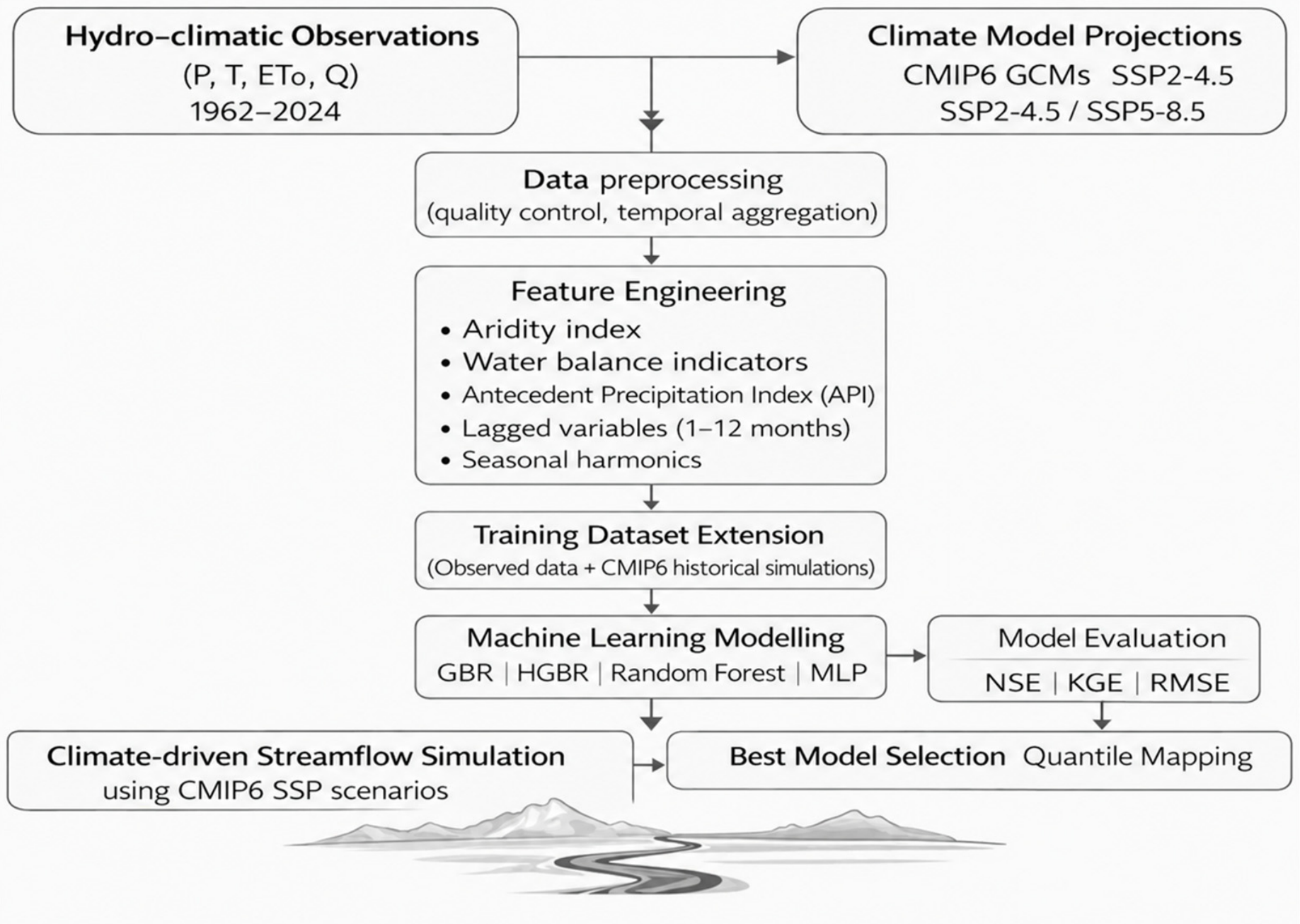
The methodological workflow combines historical hydroclimatic observations, CMIP6 climate forcing, and machine-learning techniques to simulate historical and future monthly streamflow in the Zat River Basin. The observational dataset extends from February 1962 to August 2024 and includes precipitation, air temperature, reference evapotranspiration, and discharge. Hydrologically informed feature engineering is used to derive an aridity indicator, water-balance indicators, antecedent precipitation indices, climatic interaction terms, lagged predictors up to 12 months, and harmonic variables representing seasonality [34,35].

The final rainfall–runoff models were developed using the observed hydroclimatic record. The scenario files available for this analysis begin in 2015 and therefore were not used to extend the 1962–2005 model-development sample with historical GCM simulations.

Using the resulting dataset, four machine-learning algorithms—Gradient Boosting Regressor (GBR), Histogram-based Gradient Boosting Regressor (HGBR), Random Forest (RF), and Multi-Layer Perceptron (MLP)—are trained to reproduce the rainfall–runoff relationship. Model calibration was performed over 1962–2005, while the 2006–2014 window was used for chronological validation. The predictive performance of the models was evaluated using standard hydrological indicators, including NSE, KGE, RMSE, MAE, and R² [14]. Of the tested methods, the Gradient Boosting Regressor (GBR) yielded the highest accuracy and was retained for subsequent projections. This finding agrees with the recent literature emphasizing the robustness of boosting algorithms in rainfall-runoff applications [16,36]. To further improve reliability, simulated streamflow is corrected using a monthly quantile-mapping bias correction, a widely applied method for reducing systematic biases in climate-impact studies [33]. For each model, monthly quantile-mapping transfer functions were fitted between raw simulated and observed discharge during calibration and were then applied without recalibration to validation and future simulations [28,30]. Finally, the selected model was subsequently forced with CMIP6-derived series under SSP2-4.5 and SSP5-8.5. The post-processed discharge was first evaluated without an additional temperature adjustment. The empirical runoff-temperature-sensitivity coefficient α (°C⁻¹) was then examined at 0.02, 0.04, and 0.06 as exploratory sensitivity cases; α = 0 denotes the reference case in which no additional exponential temperature adjustment is applied. The conceptual workflow can be schematically described by Figure 2.

All analyses were performed in Python 3.13.5 using NumPy 2.1.3, pandas 2.2.3, SciPy 1.15.3, scikit-learn 1.6.1, and Matplotlib 3.10.0. A fixed random seed of 42 was used for stochastic model components. The final GBR configuration used 1200 trees, a learning rate of 0.05, a maximum depth of 3, and a subsampling fraction of 0.9. To complement the chronological hold-out assessment, a three-fold expanding-window time-series diagnostic was performed within the model-development period; it was used as a robustness diagnostic rather than for model tuning.

3.2. Feature Engineering and Input Variables

To represent the complex hydroclimatic processes governing streamflow generation in the Zat River Basin, several physically meaningful predictors were derived from the original climatic variables. These predictors were designed to capture climatic water availability, atmospheric evaporative demand, catchment memory effects, delayed hydrological responses, and seasonal controls. Such processes are particularly important in semi-arid mountainous environments, where runoff is influenced by precipitation variability, evapotranspiration, snow accumulation, delayed snowmelt, and groundwater storage.

An aridity indicator was first introduced to quantify the balance between atmospheric water demand and precipitation supply (Equation (1)):

$$A{I}_t={\displaystyle \frac{ET{0}_t}{P_t+1}}$$

(1)

where $A{I}_t$ is the monthly aridity indicator at time $t$, $ET{0}_t$ is the monthly reference evapotranspiration in mm ${\mathrm{m}\mathrm{o}\mathrm{n}\mathrm{t}\mathrm{h}}^{-1}$, and $P_t$ is the monthly precipitation in mm ${\mathrm{m}\mathrm{o}\mathrm{n}\mathrm{t}\mathrm{h}}^{-1}$. The constant value of 1 mm was added to the denominator to avoid numerical instability during months with negligible or zero rainfall. High values of $A{I}_t$ indicate dry conditions where evaporative demand exceeds precipitation supply, whereas low values correspond to wetter conditions.

The climatic water surplus potentially available for runoff generation and groundwater recharge was calculated using Equation (2):

$$W_t=\mathrm{m}\mathrm{a}\mathrm{x}(P_t-ET{0}_t,0)$$

(2)

where $W_t$ represents the monthly water surplus in mm ${\mathrm{m}\mathrm{o}\mathrm{n}\mathrm{t}\mathrm{h}}^{-1}$; this variable expresses the fraction of precipitation that remains after satisfying atmospheric evaporative demand and therefore provides a simple proxy for effective moisture availability within the catchment.

Because the aridity indicator varies substantially across seasons and years, it was standardized using the z-score transformation given in Equation (3):

AI_norm,t = (AI_t − μ_AI)/σ_AI

(3)

where AI_norm,t is the standardized aridity indicator at month t, μ_AI is the mean aridity indicator over the calibration dataset, and σ_AI is the corresponding standard deviation. Positive values indicate conditions drier than the calibration period mean, whereas negative values indicate relatively wetter conditions. The transformation places the indicator on a dimensionless standardized scale and improves numerical stability; it is a z-score transformation.

Two interaction terms were generated to represent nonlinear effects between climate forcing and antecedent basin dryness (Equations (4) and (5)):

$$P_{AI,t}=P_t\times A{I}_{\mathrm{n}\mathrm{o}\mathrm{r}\mathrm{m},t}$$

(4)

$$ET{0}_{AI,t}=ET{0}_t\times A{I}_{\mathrm{n}\mathrm{o}\mathrm{r}\mathrm{m},t}$$

(5)

where $P_{AI,t}$ represents the interaction between precipitation and standardized aridity, while $ET{0}_{AI,t}$ represents the interaction between reference evapotranspiration and standardized aridity. These variables allow the models to account for the fact that the hydrological effect of a given rainfall event or evaporative demand may vary depending on the antecedent dryness of the basin.

Hydrological memory was represented using the antecedent precipitation index (API), defined in Equation (6):

$$AP{I}_t^{\left(\lambda \right)}=P_t+\lambda AP{I}_{t-1}^{\left(\lambda \right)}$$

(6)

where $AP{I}_t^{\left(\lambda \right)}$ is the antecedent precipitation index at month $t$, $AP{I}_{t-1}^{\left(\lambda \right)}$ is the value of the index during the previous month, and $\lambda$ is the recession coefficient controlling the persistence of past precipitation effects. Two values were considered, $\lambda =0.90$ and $\lambda =0.98$, representing short-term and long-term catchment memory, respectively. These indices provide a simplified representation of soil-moisture storage, groundwater recharge, and delayed runoff generation processes.

To further represent delayed hydrological responses, lagged versions of the principal predictors were generated for lags of 1–12 months. The lagged variables included precipitation, ET0, standardized aridity, water surplus, and the two interaction terms. These predictors represent antecedent climatic conditions, seasonal groundwater storage, delayed snowmelt, and subsurface contributions typical of High Atlas catchments.

Seasonality was incorporated using harmonic variables based on the calendar month (Equations (7) and (8)):

$$S_t=\sin \left({\displaystyle \frac{2\pi M_t}{12}}\right)$$

(7)

$$C_t=\cos \left({\displaystyle \frac{2\pi M_t}{12}}\right)$$

(8)

where $S_t$ and $C_t$ are the seasonal indicators, respectively, and $M_t$ denotes the month number, with $M_t=1,\dots ,12$. These cyclic variables preserve the continuity of the annual calendar and enable the models to represent recurring seasonal patterns associated with precipitation regimes, snow dynamics, evapotranspiration cycles, and seasonal runoff variability.

All predictor variables were standardized within a scikit-learn preprocessing pipeline before model calibration. To reduce heteroscedasticity and stabilize variance, the target discharge was transformed using the square-root transformation in Equation (9), and predictions were returned to physical units using the inverse transformation in Equation (10):

$$Q^{*}=\sqrt{Q}$$

(9)

where $Q^{*}$ is the transformed streamflow used during model training and $Q$ is the observed discharge in ${{\mathrm{m}}^3\mathrm{s}}^{-1}$. After prediction, the inverse transformation was applied to recover streamflow estimates in their original physical units:

$$Q=(Q^{*}{)}^2$$

(10)

Overall, these engineered predictors were designed to represent the main hydrological controls of runoff generation in the Zat River Basin, including climatic water availability, atmospheric evaporative demand, antecedent moisture conditions, catchment memory, delayed hydrological responses, and seasonal variability. By integrating both physically based and statistically derived features, the modeling framework enables machine-learning algorithms to better capture the nonlinear behavior of streamflow in semi-arid mountainous environments characterized by strong climatic variability, snow-related processes, and complex storage dynamics.

3.3. Machine-Learning Models

To capture the complex nonlinear rainfall–runoff relationships governing semi-arid mountainous basins, four supervised machine-learning regression algorithms were implemented and comparatively evaluated: Gradient Boosting Regressor (GBR), Histogram-based Gradient Boosting Regressor (HGBR), Random Forest (RF), and a Multi-Layer Perceptron neural network (MLP). These models represent complementary families of data-driven approaches commonly used in hydrological modeling and environmental prediction. Ensemble tree-based algorithms are particularly effective in capturing nonlinear interactions between hydroclimatic variables, while neural networks provide flexible function approximation capabilities suitable for complex hydrological systems [16,34,35].

The use of multiple algorithms enables a robust assessment of the ability of machine-learning techniques to reproduce rainfall–runoff dynamics, seasonal variability, and delayed catchment responses associated with snowmelt and soil-moisture storage processes [18,36].

a. 

Gradient Boosting Regressor (GBR)

Gradient Boosting Regressor is an ensemble-based approach that sequentially develops regression trees, where each successive tree is trained to correct the errors of the preceding ones through gradient-based optimization of a loss function. This progressive learning strategy enhances predictive accuracy and allows the model to capture nonlinear interactions between hydroclimatic inputs and discharge.

Boosting algorithms are effective in hydrological applications because they can represent threshold effects, variable interactions, and nonlinear rainfall–runoff responses [36,37]. In this study, the GBR model was configured with 1200 decision trees, a learning rate of 0.05, a maximum tree depth of three, and a subsampling fraction of 0.9. Subsampling was used to reduce variance and limit overfitting.

b. 

Histogram-based Gradient Boosting Regressor (HGBR)

The Histogram-based Gradient Boosting Regressor represents a computationally optimized implementation of gradient boosting. Instead of evaluating all possible split points for continuous variables, the algorithm discretizes features into histograms, which substantially reduces computational cost while maintaining predictive performance.

This approach is particularly suitable for large datasets or high-dimensional predictor spaces. The model iteratively improves prediction accuracy through gradient-based optimization while applying regularization techniques such as early stopping to prevent overfitting [38].

In the present study, the HGBR model was trained with up to 800 boosting iterations, with early stopping criteria implemented to ensure model generalization and computational efficiency.

c. 

Random Forest (RF)

Random Forest is a bagging-based ensemble method that generates multiple decision trees from bootstrap samples of the training dataset [39]. At each split, a random subset of predictors is used, reducing correlation among trees and enhancing model robustness. Final predictions are obtained by averaging across all trees, which lowers variance and improves stability. Owing to its ability to model nonlinear processes and handle noisy hydrological data, Random Forest is widely applied in hydrology [40,41]. In this work, the model was implemented with several hundred trees and no depth limitation to capture the complexity of rainfall-runoff dynamics.

d. 

Multi-Layer Perceptron (MLP)

The Multi-Layer Perceptron is a feed-forward Artificial Neural Network designed to approximate complex nonlinear functions through multiple layers of interconnected neurons. Each neuron applies a weighted transformation of its inputs followed by a nonlinear activation function.

The architecture implemented in this study consists of two hidden layers containing 80 and 40 neurons, respectively, with Rectified Linear Unit (ReLU) activation functions. Regularization was implemented through an L2 penalty to limit overfitting and improve generalization.

Neural networks have shown strong potential in hydrological modeling, particularly for capturing nonlinear dependencies and temporal interactions between climatic drivers and streamflow responses [16,18].

3.4. Performance Metrics

Model performance was evaluated using five complementary indicators. Their mathematical definitions are provided below, where $Q_{obs,i}$ and $Q_{sim,i}$ denote observed and simulated discharge at time i, ${\overline{Q}}_{obs}$ is the mean observed discharge, and n is the number of paired observations.

• Nash–Sutcliffe Efficiency (NSE)

$$NSE=1-{\displaystyle \frac{\sum (Q_{sim}-Q_{obs}{)}^2}{\sum (Q_{obs}-{\overline{Q}}_{obs}{)}^2}}$$

(11)

The Nash–Sutcliffe efficiency measures the predictive skill of the simulation relative to the observed-mean benchmark. NSE = 1 indicates perfect agreement, NSE = 0 indicates performance equivalent to the observed mean, and negative values indicate poorer performance.

• Kling–Gupta Efficiency (KGE) combines correlation, the variance ratio and bias ratio:

$$KGE=1-\sqrt{\left(r-1{)}^2+(\alpha -1{)}^2+(\beta -1{)}^2\right.}$$

(12)

where r is the Pearson correlation coefficient between observed and simulated discharge, α = σ_sim/σ_obs is the variability ratio, and β = μ_sim/μ_obs is the bias ratio. KGE jointly evaluates correlation, variability, and mean bias.

• Root Mean Square Error (RMSE) and Mean Absolute Error (MAE)

The root mean square error is expressed in the same unit as discharge and gives greater weight to large errors.

$$RMSE=\sqrt{{\displaystyle \frac{1}{n}}\sum (Q_{sim}-Q_{obs}{)}^2}$$

(13)

The mean absolute error represents the average magnitude of the simulation errors in discharge units.

$$MAE={\displaystyle \frac{1}{n}}\sum (Q_{sim}-Q_{obs})$$

(14)

• Coefficient of determination $R^2$

R² = r², where r is the Pearson linear correlation coefficient between observed and simulated discharge. R² therefore measures the strength of the linear association between the two series. Because a high R² does not by itself exclude systematic bias, it was interpreted together with NSE, KGE, RMSE, and MAE.

3.5. Monthly Quantile-Mapping Post-Processing of Simulated Streamflow

Machine-learning rainfall–runoff models may retain systematic errors in the magnitude and distribution of simulated discharge [33,42]. To reduce these residual biases, monthly quantile mapping was applied as a statistical post-processing procedure to the model output. For each calendar month m, the empirical cumulative distribution function of raw simulated discharge during calibration was mapped onto the corresponding distribution of observed discharge:

$$Q_{m,\mathrm{corr}}=F_{\mathrm{obs},m}^{-1}\left(F_{\mathrm{sim},m}\left(Q_{sim}\right)\right)$$

(15)

where $Q_{sim}$ is the raw modeled discharge and $Q_{m,\mathrm{corr}}$ is the post-processed discharge. Here, F_sim,m denotes the empirical cumulative distribution function (CDF) of raw simulated discharge for calendar month m during calibration, and F_obs,m⁻¹ denotes the inverse empirical CDF of observed discharge for the same calendar month.

The twelve-monthly transfer functions were estimated exclusively from the calibration period and then applied without recalibration to the independent validation period and future simulations. Applying the correction at monthly resolution accounts for the pronounced seasonal regime of the basin and corrects residual errors in the integrated rainfall–runoff response. In this study, quantile mapping was applied to simulated streamflow, not separately to P, T, and ET₀. Its use for future periods assumes that the historical monthly transfer functions remain sufficiently stable under changing climatic conditions.

3.6. Temperature-Driven Runoff Correction

Studies of semi-arid and snow-influenced basins indicate that warming can reduce runoff through enhanced evapotranspiration and altered snow accumulation and melt. Because temperature and ET₀ are already included among the machine-learning predictors, the exponential temperature term was treated as an exploratory sensitivity assessment rather than as a compulsory physical correction. Simulations were generated for α = 0, 0.02, 0.04, and 0.06, where $\alpha$ = 0 represents the unadjusted machine-learning projection. This design quantifies the additional effect introduced by the empirical temperature parameter and explicitly addresses the potential double counting of warming effects (Equation (16):

$$Q_{\mathrm{forced},t}=Q_{\mathrm{QM},t}\hspace{0.25em} \exp \left(-\alpha \Delta T_t\right)$$

(16)

In Equation (16), $Q_{\mathrm{QM},t}$ is the monthly discharge after quantile-mapping post-processing, $\Delta T_t$ is the temperature anomaly relative to the 1962–2005 calibration mean, and α is the runoff-temperature-sensitivity parameter. This empirical adjustment does not replace a snow or energy-balance model; it introduces a transparent sensitivity term that should be interpreted as an approximation and considered in the uncertainty analysis. The variable Q_forced,t denotes the final discharge at month t after application of the exploratory temperature-sensitivity adjustment. When α = 0, Q_forced,t = Q_QM,t, so no additional temperature adjustment is applied.

4. Results

4.1. Performance of Machine-Learning Rainfall–Runoff Models

The machine-learning rainfall–runoff models were evaluated over the 1962–2005 model-development period and a chronological 2006–2014 hold-out window using NSE, KGE, RMSE, MAE, and R². Because 12-month lags were required, the formal hold-out metrics cover January 2007 to November 2014.

Table 4. Performance metrics for the calibration period (1962–2005).

Model	NSE	KGE	RMSE	MAE	R2
GBR	0.99	0.99	0.03	0.01	0.99
HGBR	0.81	0.90	2.23	1.08	0.80
RF	0.98	0.98	0.74	0.39	0.98
MLP	0.99	0.99	0.17	0.08	0.99

and

Table 5. Performance metrics for the chronological hold-out window (2006–2014).

Model	NSE	KGE	RMSE	MAE	R2
GBR	0.71	0.80	1.61	1.17	0.72
HGBR	0.38	0.70	2.38	1.46	0.52
RF	0.52	0.76	2.10	1.35	0.62
MLP	0.10	0.51	2.87	1.82	0.47

summarize the corresponding results and provide complementary information on efficiency, correlation, variability, bias, and error magnitude.

GBR provided the best validation performance, with NSE = 0.71, KGE = 0.80, RMSE = 1.61 m³ s⁻¹, MAE = 1.17 m³ s⁻¹, and R² = 0.72. It outperformed RF (NSE = 0.52), HGBR (NSE = 0.38), and MLP (NSE = 0.10) in terms of overall predictive efficiency. These results indicate satisfactory monthly predictive skill, while also showing that performance decreased from calibration to validation. For GBR, monthly quantile mapping (QM) reduced calibration RMSE from 0.076 to 0.028 m³ s⁻¹, but it did not improve hold-out efficiency: NSE changed from 0.720 before QM to 0.714 after, while KGE remained essentially unchanged (0.798 to 0.799) and RMSE changed from 1.594 to 1.612 m³ s⁻¹. QM is therefore interpreted as a distributional post-processing step rather than as a procedure that necessarily increases out-of-sample skill.

Table 6. Effect of monthly discharge quantile mapping on GBR performance.

Period	Correction	NSE	KGE	RMSE (m3 s−1)	MAE (m3 s−1)	R2 (Pearson2)
Model development	Raw	0.9998	0.9925	0.0758	0.0504	0.9998
Model development	QM	1.0000	0.9999	0.0275	0.0137	1.0000
Chronological hold-out	Raw	0.7205	0.7981	1.5940	1.1662	0.7215
Chronological hold-out	QM	0.7142	0.7985	1.6118	1.1737	0.7157

summarizes the corresponding GBR performance metrics before and after monthly quantile mapping for the calibration and chronological hold-out periods.

All four algorithms reproduced part of the seasonal and interannual variability, but their ability to generalize differed substantially. During calibration, GBR and MLP achieved NSE values close to 1.00, RF achieved NSE = 0.98, and HGBR achieved NSE = 0.81. The marked reduction in MLP validation performance, despite its near-perfect calibration score, indicates overfitting. GBR showed the most balanced calibration–validation behavior and was therefore retained for the climate driven simulations.

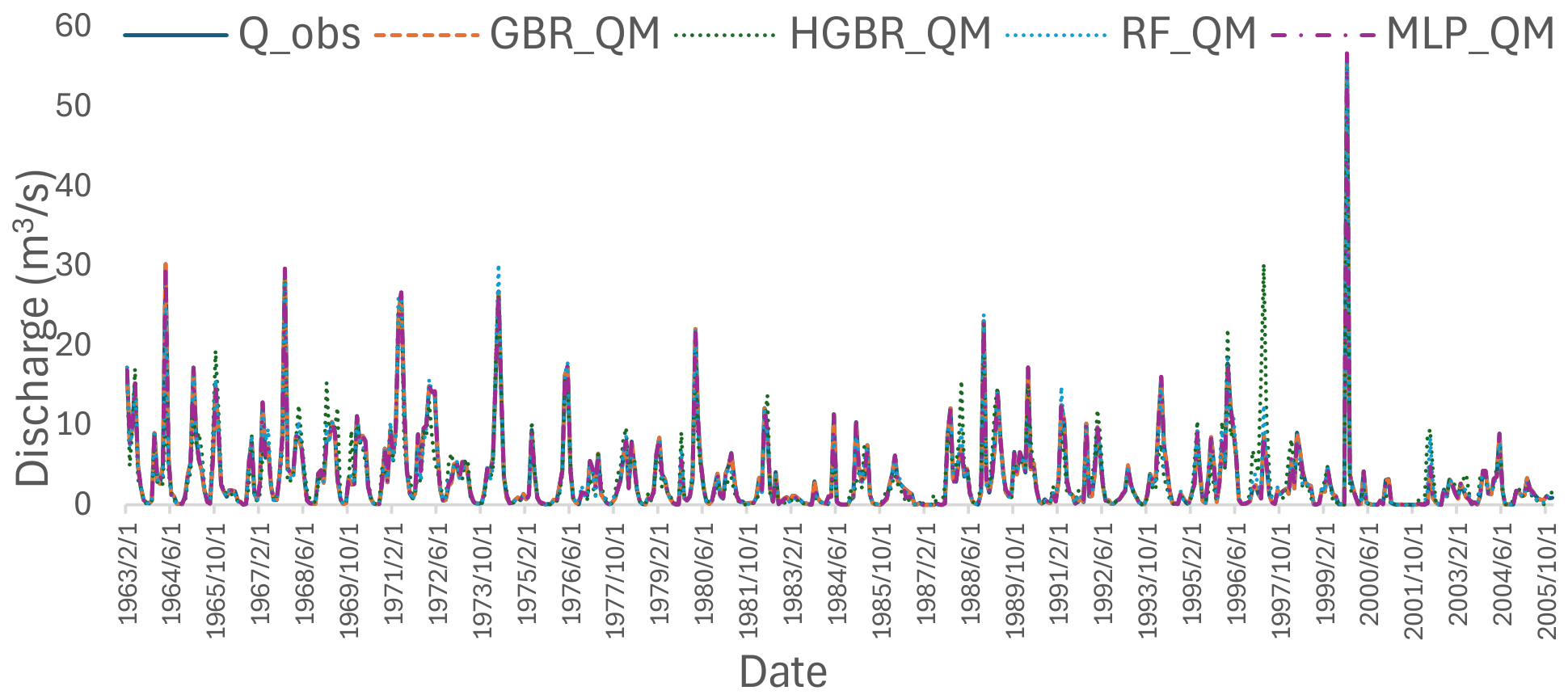
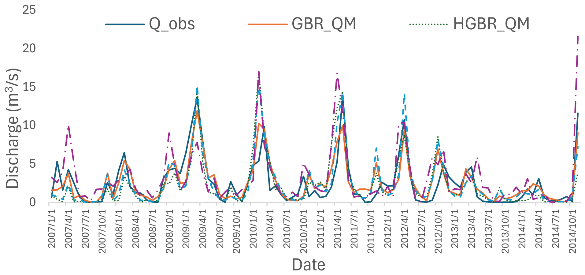
Figure 3 and Figure 4 compare observed and simulated monthly discharge during calibration and validation, respectively. The simulations reproduce the principal seasonal pattern and many high- and low-flow periods, although the agreement is visibly weaker during validation and for some peak-flow events.

Figure 3 and Figure 4 show that GBR reproduces the timing and magnitude of many monthly flow variations more consistently than the other models, including several peak and recession periods. The statistical indicators and the visual comparison jointly support its selection for future simulations. Nevertheless, the reduced validation performance relative to calibration and the remaining peak-flow errors are retained as explicit limitations.

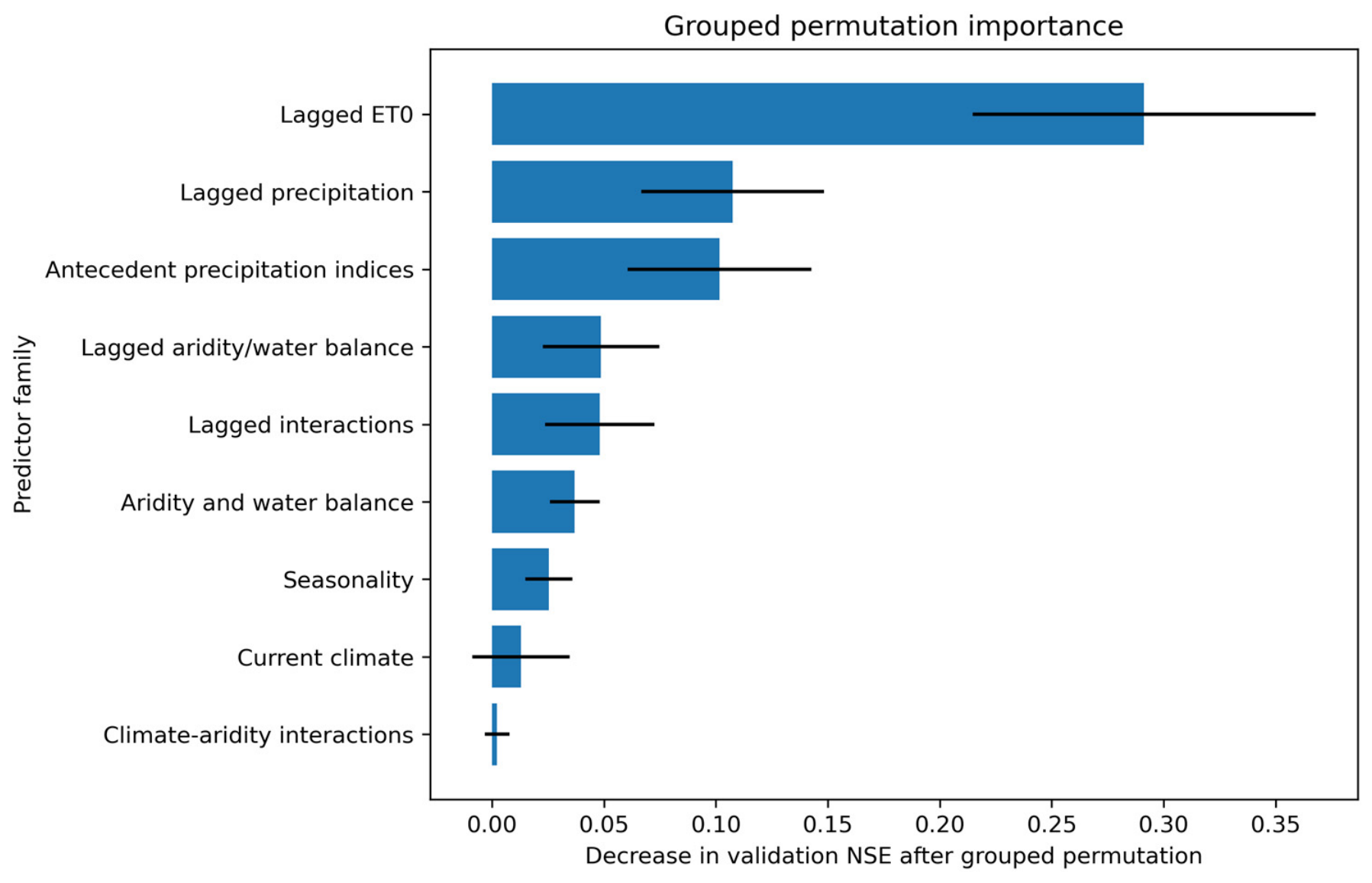
Permutation importance was evaluated on the formal validation sample using ten repeated permutations and the decrease in NSE as the scoring criterion. Lagged ET₀ was the dominant predictor family (mean NSE decrease = 0.291), followed by lagged precipitation (0.107) and the antecedent precipitation indices (0.102). At the individual variable level, ET₀ lagged by one month produced the largest decrease in validation NSE (0.243), followed by API with λ = 0.98 (0.098) and API with λ = 0.90 (0.065). These results emphasize the roles of evaporative demand, antecedent wetness, and delayed catchment response. Because several predictors are correlated, the importance values are interpreted as predictive contributions rather than direct causal effects. To further interpret the selected GBR model, Figure 5 presents the grouped permutation importance of the predictor families.

4.2. Evaluation of Climate-Driven Simulations Against Recent Observations

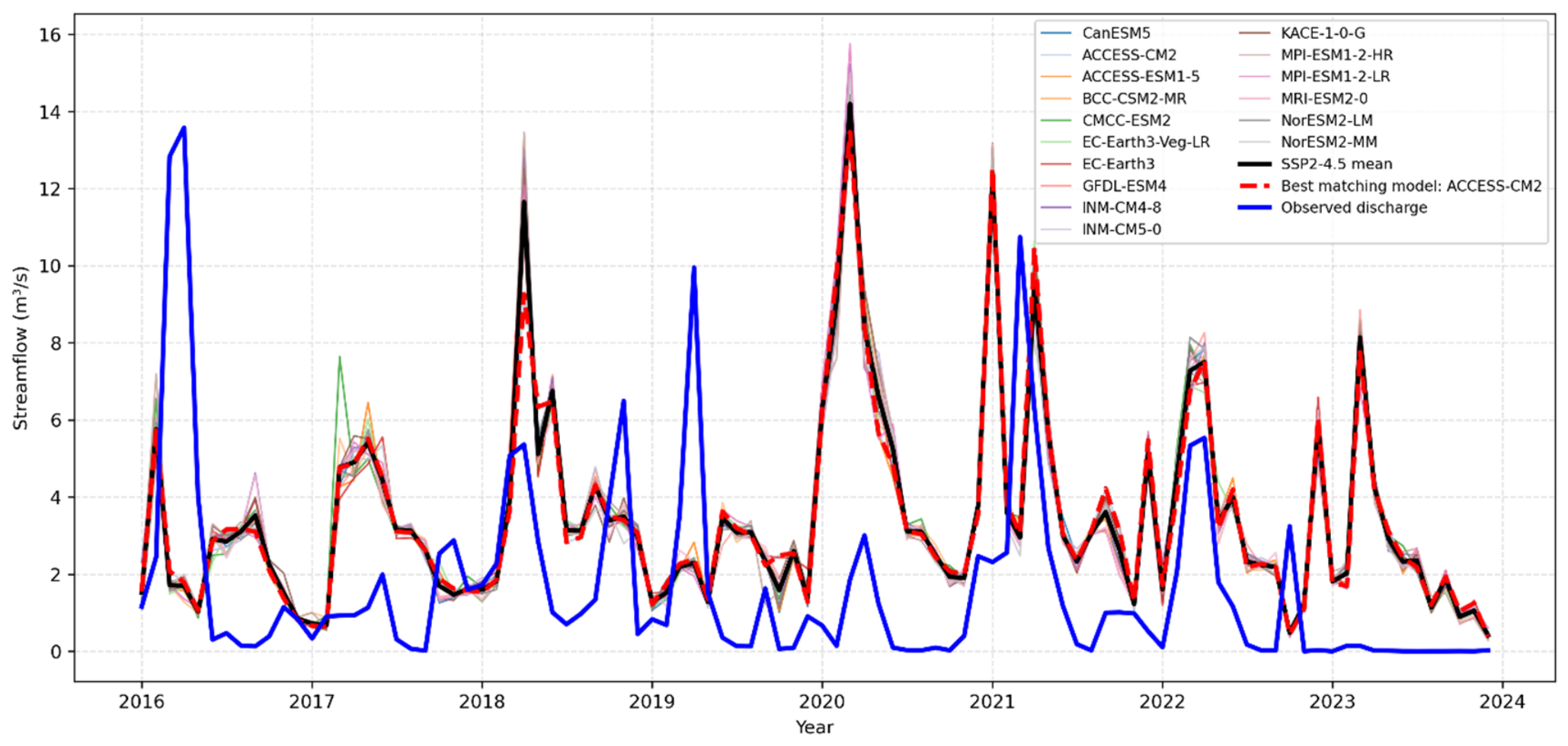
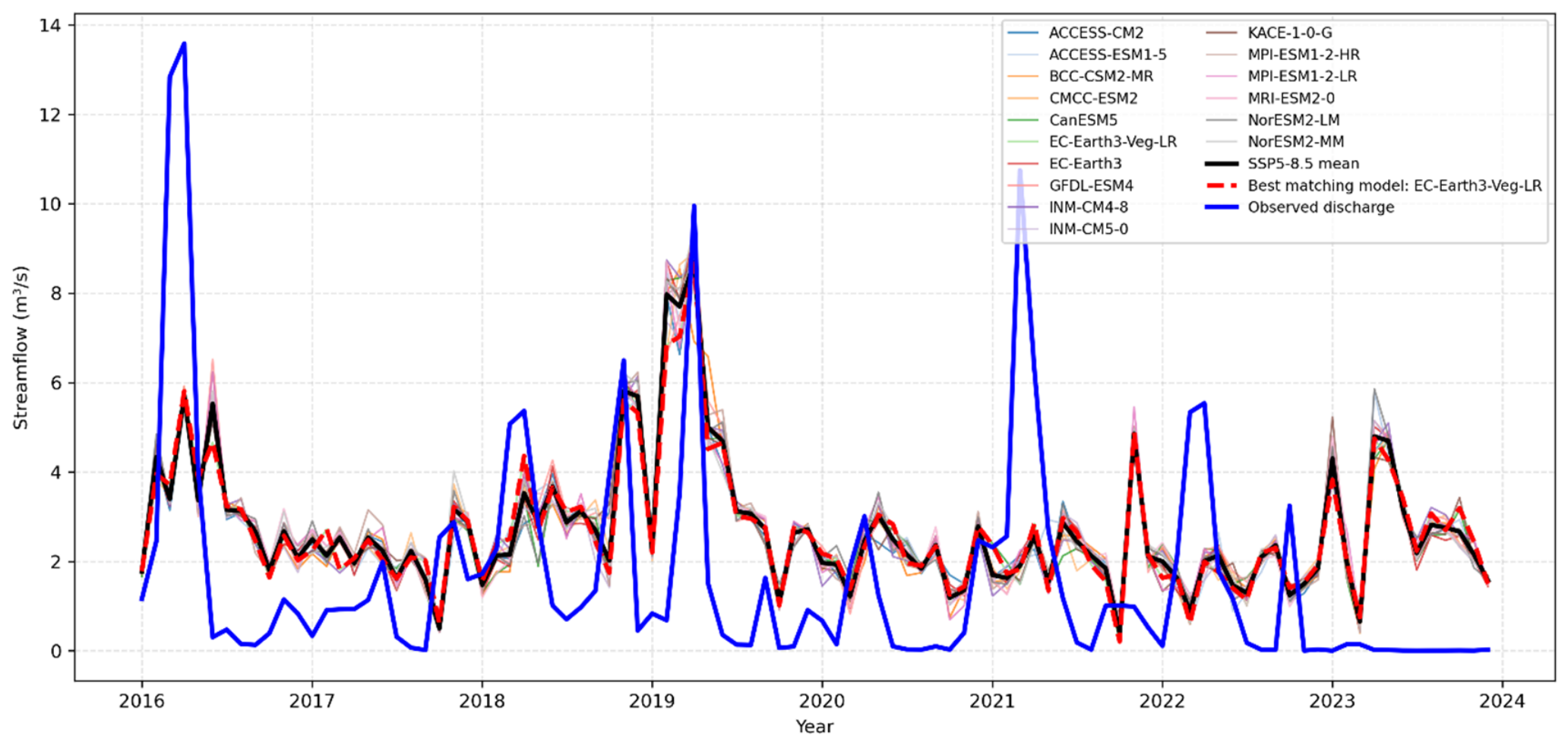
To provide a supplementary assessment over the recent period, climate-driven simulations were compared with observed monthly discharge for 2016–2024, a period that was not used in model calibration or in the formal 2006–2014 validation metrics. Figure 6 and Figure 7 show the comparisons for SSP2-4.5 and SSP5-8.5, respectively.

The multi-model climate-driven simulations reproduce the broad temporal variability of streamflow, but substantial discrepancies remain during extreme events. Under both scenarios, the ensemble mean follows the general evolution of monthly discharge, whereas the observed series contains sharper and larger peaks during several flood episodes. This behavior is consistent with the use of spatially averaged monthly climate forcing, which smooths short-duration precipitation extremes and limits the representation of peak flows.

For SSP2-4.5, ACCESS-CM2 produced the closest visual agreement with observations over 2016–2024. Under SSP5-8.5, EC-Earth3-Veg-LR was the closest individual member in Figure 6, although the spread among models was somewhat larger. These member-specific comparisons are descriptive and should not be interpreted as a formal ranking of GCM skill because the evaluation period is short and the scenarios diverge only weakly during the early decades.

Taken together, Figure 6 and Figure 7 indicate that the framework captures broad recent hydrological variability while underrepresenting some abrupt peaks. Future changes in mean and seasonal streamflow can therefore be interpreted with greater confidence than the magnitude of individual extreme-flow events.

4.3. Future Streamflow Projections Under SSP2-4.5 and SSP5-8.5

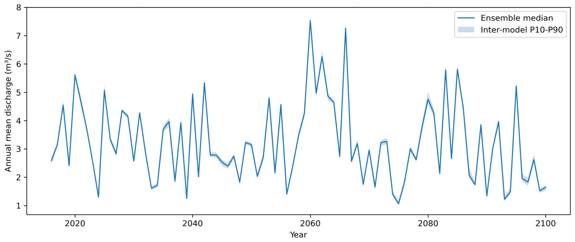
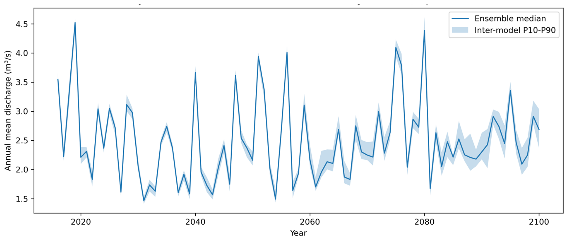
Future streamflow projections were summarized using the ensemble median and the inter-model 10th–90th percentile (P10–P90). The unadjusted machine-learning simulations (α = 0) are presented as the reference projections, while alternative α values are reported as a sensitivity range. Figure 8 and Figure 9 illustrate the projected annual streamflow evolution under SSP2-4.5 and SSP5-8.5, respectively, using the ensemble median of the 16 GCMs and the inter-model P10–P90 range to represent projection spread, with no additional temperature adjustment (α = 0).

Under SSP2-4.5, the reference simulations indicate median changes of −2.7% in 2021–2040 and −4.1% in 2041–2060. A temporary positive anomaly appears in 2061–2080 (+1.7%), followed by an end-century decline of −12.1% (P10-P90: −13.4% to −10.0%). All sixteen GCMs project a decrease during 2081–2100.

Under SSP5-8.5, the reference projections show a stronger and more persistent reduction: the median change is −30.4% in 2021–2040, −27.1% in 2041–2060, −22.4% in 2061–2080, and −27.3% in 2081–2100. The end-century P10-P90 range extends from −30.8% to −21.3%, and all ensemble members indicate lower mean discharge.

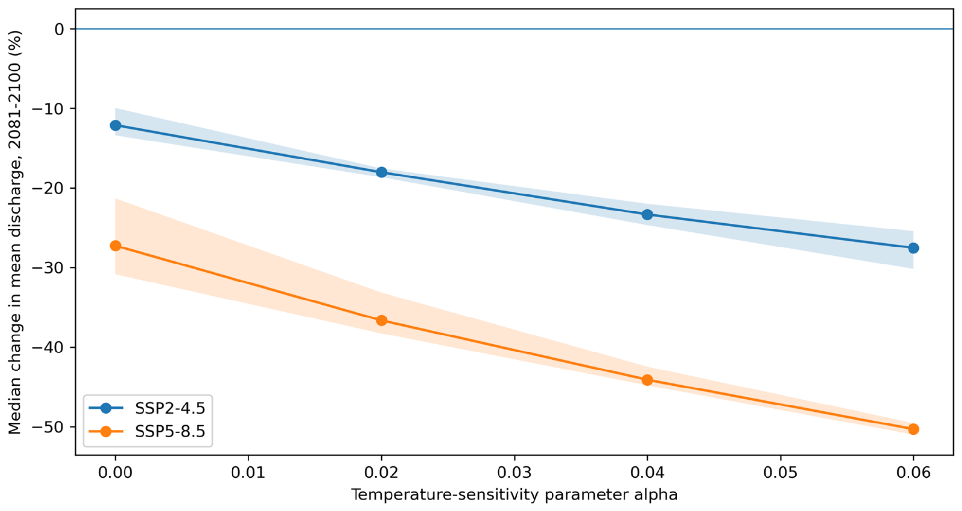
Figure 10 illustrates the sensitivity of the median end-century streamflow change (2081–2100) to the temperature-sensitivity parameter α, while the shaded P10–P90 bands represent the spread across the 16 GCMs.

The sensitivity analysis confirms that the direction of end-century change does not depend on the additional exponential adjustment, but its magnitude does. Under SSP2-4.5, the median reduction varies from −12.1% at α = 0 to −27.5% at α = 0.06. Under SSP5-8.5, it varies from −27.3% to −50.3%. For the α = 0.04 the corresponding reductions are −23.3% and −44.1%. The α adjusted values are therefore interpreted as sensitivity estimates rather than uniquely determined projections.

Table 7. Median projected streamflow changes and inter-model P10–P90 ranges under SSP2-4.5 and SSP5-8.5 for α = 0 and α = 0.04.

Scenario	Period	α = 0 Median (%)	P10–P90 (%)	α = 0.04 Median (%)	P10–P90 (%)
SSP2-4.5	2021–2040	−2.7	−3.8 to −1.9	−9.8	−10.9 to −9.2
SSP2-4.5	2041–2060	−4.1	−5.1 to −2.6	−14.4	−15.4 to −13.2
SSP2-4.5	2061–2080	1.7	0.7 to 3.5	−9.0	−11.2 to −8.1
SSP2-4.5	2081–2100	−12.1	−13.4 to −10.0	−23.3	−24.7 to −22.0
SSP5-8.5	2021–2040	−30.4	−31.7 to −29.3	−36.5	−36.7 to −36.0
SSP5-8.5	2041–2060	−27.1	−28.9 to −25.2	−37.0	−37.5 to −36.6
SSP5-8.5	2061–2080	−22.4	−24.5 to −18.2	−37.2	−37.8 to −36.6
SSP5-8.5	2081–2100	−27.3	−30.8 to −21.3	−44.1	−44.8 to −42.5

presents the projected median streamflow changes and associated inter-model P10–P90 ranges under SSP2-4.5 and SSP5-8.5 for α = 0 and α = 0.04.

5. Discussion

The results indicate a consistent tendency toward lower end-century mean streamflow, with a stronger response under SSP5-8.5. The inter-model ranges show that uncertainty affects the magnitude more than the direction of change. Without additional temperature adjustment, median reductions reach −12.1% under SSP2-4.5 and −27.3% under SSP5-8.5; the α = 0.04 sensitivity case increases these values to −23.3% and −44.1%. Milano et al. [43] reported decreases of approximately 25–50% in freshwater availability across much of the Mediterranean by 2050, with reductions exceeding 50% in some Moroccan and North African catchments. The unadjusted SSP2-4.5 estimate for the Zat Basin is below that regional range, the unadjusted SSP5-8.5 estimate lies within it, and the α = 0.04 SSP5-8.5 sensitivity estimate approaches its upper part. Mastrotheodoros et al. [13] also found that warming-related evapotranspiration feedback amplified an Alpine runoff deficit by 32% during a major heatwave, supporting the sensitivity of mountain runoff to warming, although the basin, event scale, and modeling framework differ from those used here.

The additional diagnostics also qualify the apparent model robustness. Expanding-window time-series tests within the development period produced strongly variable NSE values, revealing sensitivity to hydroclimatic regime shifts and extreme-event composition. The formal chronological hold-out remains more favorable (NSE = 0.714 after QM), but the contrast confirms that the near-perfect calibration score should not be interpreted as uniform temporal transferability. Similarly, the poor event-scale agreement during 2016–August 2024 reflects limitations of the complete climate-driven chain rather than the rainfall–runoff model alone.

The feature-importance results provide a physically coherent interpretation of the data-driven model: lagged ET₀, antecedent precipitation indices, and lagged precipitation dominate the predictive signal, supporting the roles of evaporative demand, catchment wetness, and delayed runoff generation. Nevertheless, these predictors are proxies and do not explicitly resolve snow-water equivalent, energy-balance snowmelt, groundwater storage, or surface–groundwater exchange. Quantile mapping reduces residual distributional bias in simulated discharge but assumes temporal stability of the monthly transfer functions, while the α analysis shows that additional temperature adjustment is a major source of structural uncertainty.

Compared with physically based rainfall–runoff models, the present machine-learning framework requires fewer explicit assumptions about internal process equations and can efficiently represent nonlinear relations among the available predictors. Conversely, it provides less direct process interpretability, does not explicitly conserve mass or energy, and is more dependent on the range of the training data. The two model classes should therefore be viewed as complementary. A direct benchmark against a calibrated conceptual or physically based model would strengthen future work.

The projected decline can be related to the hydrological functioning of semi-arid mountain basins. In the High Atlas, the seasonal snowpack acts as a natural reservoir by storing part of the winter precipitation and releasing water during spring and early summer [44,45]. Under warmer conditions, a larger fraction of cold-season precipitation may fall as rain, snow accumulation may decrease, and snowmelt may occur earlier [1,13]. These changes can weaken seasonal storage and reduce delayed water release during the dry season, contributing to lower spring and annual discharge.

The findings point to a marked decline in future streamflow within the Zat River Basin under projected climate conditions. For the unadjusted reference (α = 0), the ensemble median indicates end-century discharge reductions of 12.1% under SSP2-4.5 and 27.3% under SSP5-8.5 relative to the historical observed baseline. In the α = 0.04 sensitivity case, the corresponding reductions reach 23.3% and 44.1%, respectively. These results indicate a robust drying tendency, while the magnitude of the projected decline remains sensitive to the treatment of temperature effects.

Rising temperature and evaporative demand reduce effective water availability and soil-moisture storage. In a semi-arid mountain basin, relatively small changes in temperature or precipitation can therefore produce amplified changes in runoff. The projected response is consistent with the concept of runoff elasticity, whereby proportional changes in runoff may exceed proportional changes in precipitation [46,47,48]. At the same time, the simulations retain episodic high-flow events, suggesting a regime with lower mean discharge but continued exposure to extremes [49].

The magnitude of the projected reductions is broadly consistent with previous work in Morocco and the Mediterranean. Arjdal et al. [9] reported decreasing water availability under CMIP6 projections for Morocco and North Africa. Tramblay et al. [50] highlighted the sensitivity of Moroccan catchments to uncertainties in rainfall forcing, while Milano et al. [43] emphasized the role of increasing evaporative demand in future Mediterranean water balances. The present estimates should nevertheless be interpreted in relation to the specific characteristics of the Zat Basin and the assumptions of the modeling chain.

The drying tendency is also consistent with the identification of the Mediterranean as a climate-change hotspot. Large-scale circulation changes, including expansion of the Hadley circulation and shifts in mid-latitude storm tracks, may contribute to declining effective precipitation and increasing evaporative demand [10,51,52,53]. These processes can reduce river discharge, soil moisture, and groundwater recharge across semi-arid regions [53].

Several uncertainty sources must be acknowledged. First, GCMs differ in their representation of regional precipitation, temperature, and mountain-scale processes. Second, monthly and spatially averaged forcing cannot fully represent short-duration convective rainfall or flood peaks. Third, machine-learning models depend on statistical relationships learned from historical data and may have limited extrapolation capacity under non-stationary conditions [16,17,20].

Fourth, applying historical monthly quantile-mapping transfer functions to future discharge assumes that the model-error relationship remains sufficiently stable. Fifth, the empirical temperature adjustment simplifies snow and energy-balance processes. Finally, the divergence between SSP2-4.5 and SSP5-8.5 reflects uncertainty in future socioeconomic development and greenhouse-gas emissions [10,30].

Despite these limitations, the use of sixteen climate models, chronological hold-out assessment, multiple performance criteria, and explicit post-processing provides a structured basis for assessing potential hydrological change in a data-constrained basin. The projected reductions in mean discharge could substantially affect irrigation supply, groundwater recharge, and downstream water allocation, particularly under SSP5-8.5 and the higher temperature-sensitivity cases. The results therefore support adaptive planning while emphasizing that ensemble ranges, methodological assumptions, and the lower confidence associated with individual extreme events should accompany any management interpretation.

6. Conclusions

This study assessed future streamflow in the Zat River Basin using machine-learning rainfall–runoff models forced by a sixteen-member CMIP6 ensemble. Monthly quantile mapping was applied only as a post-processing correction to simulated discharge. GBR provided the best chronological validation performance, although supplementary temporal diagnostics revealed sensitivity to hydroclimatic non-stationarity. The unadjusted reference projections indicate median end-century reductions of 12.1% under SSP2-4.5 and 27.3% under SSP5-8.5. The α = 0.04 sensitivity case increases these reductions to 23.3% and 44.1%, respectively, demonstrating that the drying direction is robust while its magnitude remains method-dependent.

The projections consistently indicate lower end-century mean discharge, particularly under SSP5-8.5, but the magnitude varies across GCMs and temperature-sensitivity assumptions. This uncertainty should be considered explicitly in adaptation planning, together with the model’s reduced ability to reproduce individual flood peaks and hydroclimatic regime shifts.

These outcomes are consistent with previous studies conducted in Morocco and across the Mediterranean region, as well as with the broader findings of the IPCC AR6, which identify semi-arid regions as particularly vulnerable to future hydrological changes.

The projected decline in streamflow has important implications for water-resource management, especially in areas where demand is already high and strongly dependent on surface water. In this context, enhancing climate-resilient management strategies, improving water-use efficiency, and strengthening hydrological monitoring systems will be essential to address future climate variability.

This work demonstrates the value of combining long hydroclimatic records, hydrologically informed feature engineering, machine-learning models, and multi-model climate forcing for data-constrained mountain basins. Future research should compare the framework directly with conceptual and physically based rainfall–runoff models, test alternative bias-correction and post-processing strategies, incorporate higher-resolution precipitation and snow information, and evaluate potential land-use and water-management changes.

References

1. Beniston, M.; Farinotti, D.; Stoffel, M.; Andreassen, L.M.; Coppola, E.; Eckert, N.; Fantini, A.; Giacona, F.; Hauck, C.; Huss, M.; et al. The European mountain cryosphere: A review of its current state. trends, and future challenges. Cryosphere 2018, 12, 759–794. [Google Scholar] [CrossRef] [Scilit]
2. Viviroli, D.; Archer, D.R.; Buytaert, W.; Fowler, H.J.; Greenwood, G.B.; Hamlet, A.F.; Huang, Y.; Koboltschnig, G.; Litaor, M.I.; López-Moreno, J.I.; et al. Climate change and mountain water resources: Overview and recommendations for research. management and policy. Hydrol. Earth Syst. Sci. 2011, 15, 471–504. [Google Scholar] [CrossRef] [Scilit]
3. Boudhar, A.; Hanich, L.; Boulet, G.; Duchemin, B.; Berjamy, B.; Chehbouni, A. Evaluation of the Snowmelt Runoff Model in the Moroccan High Atlas Mountains using two snow-cover estimates. Hydrol. Sci. J. 2009, 54, 1094–1113. [Google Scholar] [CrossRef] [Scilit]
4. Chaponnière, A.; Boulet, G.; Chehbouni, A.; Aresmouk, M. Understanding hydrological processes with scarce data in a mountain environment. Hydrol. Process. 2008, 22, 1908–1921. [Google Scholar] [CrossRef] [Scilit]
5. Baba, M.W.; Gascoin, S.; Kinnard, C.; Marchane, A.; Hanich, L. Effect of digital elevation model resolution on the simulation of the snow cover evolution in the High Atlas. Water Resour. Res. 2019, 55, 5360–5378. [Google Scholar] [CrossRef] [Scilit]
6. Marchane, A.; Jarlan, L.; Hanich, L.; Boudhar, A.; Gascoin, S.; Tavernier, A.; Filali, N.; Le Page, M.; Hagolle, O.; Berjamy, B. Assessment of daily MODIS snow cover products to monitor snow cover dynamics over the Moroccan Atlas mountain range. Remote Sens. Environ. 2015, 160, 72–86. [Google Scholar] [CrossRef] [Scilit]
7. Schilling, J.; Freier, K.P.; Hertig, E.; Scheffran, J. Climate change, vulnerability and adaptation in North Africa with focus on Morocco. Agric. Ecosyst. Environ. 2012, 156, 12–26. [Google Scholar] [CrossRef] [Scilit]
8. Plan Directeur des Aménagements Intégrés des Bassins Tensift, Ksob et Igouzoulen; Agence du Bassin Hydraulique du Tensift: Marrakech, Morocco, 2022.
9. Arjdal, K.; Driouech, F.; Vignon, É.; Chéruy, F.; Manzanas, R.; Drobinski, P.; Chehbouni, A.; Idelkadi, A. Future of land surface water availability over the Mediterranean basin and North Africa: Analysis and synthesis from the CMIP6 exercise. Atmos. Sci. Lett. 2023, 24, e1180. [Google Scholar] [CrossRef] [Scilit]
10. Intergovernmental Panel on Climate Change (IPCC). Climate Change 2021: The Physical Science Basis. Contribution of Working Group I to the Sixth Assessment Report of the Intergovernmental Panel on Climate Change; Cambridge University Press: Cambridge, UK, 2023. [Google Scholar] [CrossRef] [Scilit]
11. Knutti, R.; Sedláček, J. Robustness and uncertainties in the new CMIP5 climate model projections. Nat. Clim. Change 2013, 3, 369–373. [Google Scholar] [CrossRef] [Scilit]
12. Huning, L.S.; AghaKouchak, A. Approaching 80 years of snow water equivalent information by merging different data streams. Sci. Data 2020, 7, 333. [Google Scholar] [CrossRef]
13. Mastrotheodoros, T.; Pappas, C.; Molnar, P.; Burlando, P.; Manoli, G.; Parajka, J.; Rigon, R.; Szeles, B.; Bottazzi, M.; Hadjidoukas, P.; et al. More green and less blue water in the Alps during warmer summers. Nat. Clim. Change 2020, 10, 155–161. [Google Scholar] [CrossRef] [Scilit]
14. Gupta, H.V.; Kling, H.; Yilmaz, K.; Martinez, G. Decomposition of the mean squared error and NSE performance criteria. J. Hydrol. 2009, 377, 80–91. [Google Scholar] [CrossRef] [Scilit]
15. Hrachowitz, M.; Savenije, H.H.G.; Bloschl, G.; Mcdonnell, J.J.; Sivapalan, M.; Pomeroy, J.W.; Arheimer, B.; Blume, T.; Clark, M.P.; Ehret, U.; et al. A decade of Predictions in Ungauged Basins (PUB). Hydrol. Sci. J. 2013, 58, 1198–1255. [Google Scholar] [CrossRef] [Scilit]
16. Nearing, G.S.; Kratzert, F.; Sampson, A.K.; Pelissier, C.S.; Klotz, D.; Frame, J.M.; Prieto, C.; Gupta, H.V. What role does hydrological science play in the age of machine learning? Water Resour. Res. 2021, 57, e2020WR028091. [Google Scholar] [CrossRef] [Scilit]
17. Shen, C.; Appling, A.P.; Gentine, P.; Bandai, T.; Gupta, H.; Tartakovsky, A.; Baity-Jesi, M.; Fenicia, F.; Kifer, D.; Li, L.; et al. Differentiable modelling to unify machine learning and physical models for geosciences. Nat. Rev. Earth Environ. 2023, 4, 552–567. [Google Scholar] [CrossRef] [Scilit]
18. Kratzert, F.; Klotz, D.; Brenner, C.; Schulz, K.; Herrnegger, M. Rainfall–runoff modelling using Long Short-Term Memory (LSTM) networks. Hydrol. Earth Syst. Sci. 2018, 22, 6005–6022. [Google Scholar] [CrossRef] [Scilit]
19. Nearing, G.S.; Kratzert, F.; Shalev, G.; Klotz, D.; Gauch, M.; Gilon, O. Benchmarking machine learning hydrology models for rainfall-runoff prediction. Water Resour. Res. 2023, 59, e2022WR033217. [Google Scholar]
20. Reichstein, M.; Camps-Valls, G.; Stevens, B.; Jung, M.; Denzler, J.; Carvalhais, N.; Prabhat. Deep learning and process understanding for data-driven Earth system science. Nature 2019, 566, 195–204. [Google Scholar] [CrossRef] [Scilit] [PubMed]
21. Kratzert, F.; Klotz, D.; Shalev, G.; Klambauer, G.; Hochreiter, S.; Nearing, G. Towards learning universal, regional, and local hydrological behaviors via machine learning applied to large-sample datasets. Hydrol. Earth Syst. Sci. 2019, 23, 5089–5110. [Google Scholar] [CrossRef] [Scilit]
22. Cheng, M.; Fang, F.; Kinouchi, T.; Navon, I.M.; Pain, C.C. Long lead-time daily and monthly streamflow forecasting using machine learning methods. J. Hydrol. 2020, 590, 125376. [Google Scholar] [CrossRef] [Scilit]
23. Kumar, V.; Kedam, N.; Sharma, K.V.; Mehta, D.J.; Caloiero, T. Advanced Machine Learning Techniques to Improve Hydrological Prediction: A Comparative Analysis of Streamflow Prediction Models. Water 2023, 15, 2572. [Google Scholar] [CrossRef] [Scilit]
24. Nifa, K.; Boudhar, A.; Ouatiki, H.; Elyoussfi, H.; Bargam, B.; Chehbouni, A. Deep Learning Approach with LSTM for Daily Streamflow Prediction in a Semi-Arid Area: A Case Study of Oum Er-Rbia River Basin, Morocco. Water 2023, 15, 262. [Google Scholar] [CrossRef] [Scilit]
25. Boudhar, A.; Boulet, G.; Hanich, L.; Sicart, J.E.; Chehbouni, A. Energy fluxes and melt rate of a seasonal snow cover in the Moroccan High Atlas. Hydrol. Sci. J. 2016, 61, 931–943. [Google Scholar] [CrossRef] [Scilit]
26. Abatzoglou, J.T.; Dobrowski, S.Z.; Parks, S.A.; Hegewisch, K.C. TerraClimate, a high-resolution global dataset of monthly climate and climatic water balance from 1958–2015. Sci. Data 2018, 5, 170191. [Google Scholar] [CrossRef] [Scilit] [PubMed]
27. McNally, A.; Arsenault, K.; Kumar, S.; Shukla, S.; Peterson, P.; Wang, S.; Funk, C.; Peters-Lidard, C.D.; Verdin, J.P. A land data assimilation system for sub-Saharan Africa food and water security applications. Sci. Data 2017, 4, 170012. [Google Scholar] [CrossRef] [Scilit] [PubMed]
28. Eyring, V.; Bony, S.; Meehl, G.A.; Senior, C.A.; Stevens, B.; Stouffer, R.J.; Taylor, K.E. Overview of the Coupled Model Intercomparison Project Phase 6 (CMIP6). Geosci. Model Dev. 2016, 9, 1937–1958. [Google Scholar] [CrossRef] [Scilit]
29. Nikulin, G.; Jones, C.; Giorgi, F.; Asrar, G.; Büchner, M.; Cerezo-Mota, R.; Christensen, O.B.; Déqué, M.; Fernandez, J.; Hänsler, A.; et al. Precipitation climatology in an ensemble of CORDEX-Africa regional climate simulations. J. Clim. 2012, 25, 6057–6078. [Google Scholar] [CrossRef] [Scilit]
30. O’Neill, B.C.; Tebaldi, C.; van Vuuren, D.P.; Eyring, V.; Friedlingstein, P.; Hurtt, G.; Knutti, R.; Kriegler, E.; Lamarque, J.-F.; Lowe, J.; et al. The Scenario Model Intercomparison Project (ScenarioMIP) for CMIP6. Geosci. Model Dev. 2016, 9, 3461–3482. [Google Scholar] [CrossRef] [Scilit]
31. Allen, R.G.; Pereira, L.S.; Raes, D.; Smith, M. Crop Evapotranspiration—FAO Irrigation and Drainage Paper 56; FAO: Rome, Italy, 1998. [Google Scholar]
32. Hargreaves, G.H.; Samani, Z. Reference crop evapotranspiration from temperature data. Appl. Eng. Agric. 1985, 1, 96–99. [Google Scholar] [CrossRef] [Scilit]
33. Teutschbein, C.; Seibert, J. Bias correction of regional climate simulations for hydrological studies. Hydrol. Earth Syst. Sci. 2012, 16, 2649–2662. [Google Scholar] [CrossRef] [Scilit]
34. Shen, C. A transdisciplinary review of deep learning research and its relevance for water resources scientists. Water Resour. Res. 2018, 54, 8558–8593. [Google Scholar] [CrossRef] [Scilit]
35. Solomatine, D.; See, L.; Abrahart, R. Data-Driven Modelling: Concepts, Approaches and Experiences; Springer: Berlin/Heidelberg, Germany, 2010. [Google Scholar] [CrossRef] [Scilit]
36. Feng, D.; Fang, K.; Shen, C. Enhancing streamflow forecast and extracting insights using long-short term memory networks with data integration at continental scales. Water Resour. Res. 2020, 56, 9. [Google Scholar] [CrossRef] [Scilit]
37. Friedman, J.H. Greedy function approximation: A gradient boosting machine. Ann. Stat. 2001, 29, 1189–1232. [Google Scholar] [CrossRef] [Scilit]
38. Ke, G.; Meng, Q.; Finley, T.; Wang, T.; Chen, W.; Ma, W.; Ye, Q.; Liu, T.Y. LightGBM: A highly efficient gradient boosting decision tree. Adv. Neural Inf. Process. Syst. 2017, 30, 3146–3154. [Google Scholar]
39. Breiman, L. Random forests. Mach. Learn. 2001, 45, 5–32. [Google Scholar] [CrossRef] [Scilit]
40. Cutler, D.R.; Edwards, T.C., Jr.; Beard, K.H.; Cutler, A.; Hess, K.T.; Gibson, J.; Lawler, J.J. Random forests for classification in ecology. Ecology 2007, 88, 2783–2792. [Google Scholar] [CrossRef] [Scilit] [PubMed]
41. Tyralis, H.; Papacharalampous, G.; Langousis, A. A brief review of random forests for water scientists and practitioners. Water 2019, 11, 910. [Google Scholar] [CrossRef] [Scilit]
42. Maraun, D. Bias Correcting Climate Change Simulations—A Critical Review. Curr. Clim. Change Rep. 2016, 2, 211–220. [Google Scholar] [CrossRef] [Scilit]
43. Milano, M.; Ruelland, D.; Fernandez, S.; Dezetter, A.; Fabre, J.; Servat, E.; Fritsch, J.-M.; Ardoin-Bardin, S.; Thivet, G. Current state of Mediterranean water resources and future trends under climatic and anthropogenic changes. Hydrol. Sci. J. 2013, 58, 498–518. [Google Scholar] [CrossRef] [Scilit]
44. Barnett, T.; Adam, J.; Lettenmaier, D. Potential impacts of a warming climate on water availability in snow-dominated regions. Nature 2005, 438, 303–309. [Google Scholar] [CrossRef] [Scilit] [PubMed]
45. Viviroli, D.; Dürr, H.H.; Messerli, B.; Meybeck, M.; Weingartner, R. Mountains of the world, water towers for humanity: Typology, mapping, and global significance. Water Resour. Res. 2007, 43, W07447. [Google Scholar] [CrossRef] [Scilit]
46. Chiew, F.H.S. Estimation of rainfall elasticity of streamflow in Australia. Hydrol. Sci. J. 2006, 51, 613–625. [Google Scholar] [CrossRef] [Scilit]
47. Dooge, J.C.I.; Bruen, M.; Parmentier, B. A simple model for estimating the sensitivity of runoff to long-term changes in precipitation without a change in vegetation. Adv. Water Resour. 1999, 23, 153–163. [Google Scholar] [CrossRef] [Scilit]
48. Schaake, J.S. From climate to flow. In Climate Change and US Water Resources; Waggoner, P.E., Ed.; John Wiley: New York, NY, USA, 1990; pp. 177–206. [Google Scholar]
49. Fowler, H.J.; Lenderink, G.; Prein, A.F.; Westra, S.; Allan, R.P.; Ban, N.; Barbero, R.; Berg, P.; Blenkinsop, S.; Do, H.X.; et al. Anthropogenic intensification of short-duration rainfall extremes. Nat. Rev. Earth Environ. 2021, 2, 107–122. [Google Scholar] [CrossRef] [Scilit]
50. Tramblay, Y.; Thiemig, V.; Dezetter, A.; Hanich, L. Evaluation of satellite-based rainfall products for hydrological modelling in Morocco. Hydrol. Sci. J. 2016, 61, 2509–2519. [Google Scholar] [CrossRef] [Scilit]
51. Giorgi, F.; Jones, C.; Asrar, G.R. Addressing climate information needs at the regional level: The CORDEX framework. World Meteorol. Organ. (WMO) Bull. 2009, 58, 175. [Google Scholar]
52. Giorgi, F.; Lionello, P. Climate change projections for the Mediterranean region. Glob. Planet. Change 2008, 63, 90–104. [Google Scholar] [CrossRef] [Scilit]
53. Gudmundsson, L.; Kirchner, J.; Gädeke, A.; Noetzli, J.; Biskaborn, B.K. Attributing observed permafrost warming in the northern hemisphere to anthropogenic climate change. Environ. Res. Lett. 2022, 17, 095014. [Google Scholar] [CrossRef] [Scilit]
Figure 1. Location and physiographic setting of the Zat River Basin.
Atmosphere 17 00841 g001
Figure 2. Integrated climate-hydrology workflow for future streamflow projections in the Zat River Basin.
Atmosphere 17 00841 g002
Figure 3. Observed and simulated monthly discharge during the calibration period (1962–2005).
Atmosphere 17 00841 g003
Figure 4. Observed and simulated monthly discharge during the chronological hold-out period (2006–2014).
Atmosphere 17 00841 g004
Figure 5. Grouped permutation importance of the selected GBR model. Error bars show the standard deviation across ten repetitions.
Atmosphere 17 00841 g005
Figure 6. Observed and climate-driven monthly discharge for 2016–2024 under SSP2-4.5.
Atmosphere 17 00841 g006
Figure 7. Observed and climate-driven monthly discharge for 2016–2024 under SSP5-8.5.
Atmosphere 17 00841 g007
Figure 8. Annual ensemble-median streamflow under SSP2-4.5 without additional temperature adjustment (α = 0). The shaded band represents the inter-model P10–P90 range.
Atmosphere 17 00841 g008
Figure 9. Annual ensemble-median streamflow under SSP5-8.5 without additional temperature adjustment (α = 0). The shaded band represents the inter-model P10-P90 range.
Atmosphere 17 00841 g009
Figure 10. Sensitivity of the median end-century streamflow change (2081–2100) to the temperature-sensitivity parameter α. Shaded bands show the inter-model P10–P90 range.
Atmosphere 17 00841 g010