Article

Spatiotemporal Variations and Trends in Tropospheric NO2 over Chongqing, a Mountainous Megacity in Southwest China, Based on Sentinel-5P TROPOMI Observations (2019–2024)

1
School of Atmospheric Physics, Nanjing University of Information Science & Technology, Nanjing 210044, China
2
China Meteorological Administration Aerosol-Cloud and Precipitation Key Laboratory, CMAWMC-NUIST Innovation Research Institute of Weather Modification, Nanjing University of Information Science & Technology, Nanjing 210044, China
3
Key Laboratory for Aerosol-Cloud-Precipitation of China Meteorological Administration, Nanjing University of Information Science & Technology, Nanjing 210044, China
*
Author to whom correspondence should be addressed.
Atmosphere 2026, 17(8), 791; https://doi.org/10.3390/atmos17080791
Submission received: 19 July 2026 / Revised: 14 August 2026 / Accepted: 17 August 2026 / Published: 18 August 2026
(This article belongs to the Section Air Quality)

Abstract

Nitrogen dioxide (NO2) drives ozone and secondary aerosol formation and harms human health. Chongqing, a mountainous megacity of 32 million people, lacks a fine-scale satellite assessment of its NO2 evolution. We analyzed tropospheric NO2 vertical column density (VCD) over Chongqing for 2019–2024. The analysis used Sentinel-5P TROPOMI observations. We computed monthly, seasonal, and annual composites at 5.5 km resolution. Trends were quantified with the Theil–Sen slope and, at the pixel level, the Seasonal Mann–Kendall (SMK) test applied to the full 72-month series. A MODIS land-cover mask separated urban built-up from non-urban pixels. NO2 concentrated in the central districts and along the Yangtze valley. The core exceeded the mountainous counties by a factor of 3 to 4. TROPOMI resolved the Wanzhou and Yongchuan–Jiangjin hotspots as separate features. The record was divided into three phases. The 2020 lockdown produced the minimum, 31% below the prior February. Rebound emissions produced the 2021 maximum of 5.6 × 10¹⁵ molecules cm−2 under near-normal dispersion conditions, with ERA5 (the European Centre of Medium-range Weather Forecasts Reanalysis v.5) showing the January 2021 boundary layer 4.3% deeper than its climatological norm. Thereafter the regional mean stabilized: the area-weighted SMK slope was +0.042 × 10¹⁵ molecules cm−2 yr−1 and not significant (p = 0.14), because emission controls in the core and rising county emissions canceled in the average. Trends diverged sharply in space. The nine core districts declined (median urban Sen slope −0.11 × 10¹⁵ molecules cm−2 yr−1), whereas 41% of peripheral pixels rose significantly (p < 0.05). The urban-to-rural ratio narrowed from 3.0 in 2019 to 2.3 in 2024 (annual means). This convergence was robust to the built-up threshold (30–50%). Industrial relocation and county urbanization explain the peripheral rise. The results support extending vehicle and industrial emission standards from the core to the receiving counties.

1. Introduction

Nitrogen dioxide (NO2) occupies a central place in tropospheric chemistry. It feeds ozone production, forms nitrate aerosol, and contributes to acid deposition [1,2]. Photolysis of NO2 supplies the only major daytime source of tropospheric ozone. Its oxidation product, nitric acid, partitions into particles and adds to PM2.5 mass [3,4]. Epidemiological work links NO2 exposure to asthma, impaired lung development, and cardiovascular mortality [5,6]. A global assessment attributed about four million new pediatric asthma cases per year to ambient NO2 [5]. Combustion dominates the sources. Vehicles, power plants, and industrial boilers emit nitrogen oxides (NOx), which cycle into NO2 within minutes [3]. Soil emissions and lightning add smaller shares outside cities. The short lifetime of NO2, hours in summer and about a day in winter, keeps the gas close to its sources [7,8]. Column NO2 therefore maps emission patterns with little smearing. This property makes NO2 the preferred satellite tracer for combustion activity in cities [9].
Satellite instruments have tracked tropospheric NO2 for three decades. GOME (Global Ozone Monitoring Experiment) began the record in 1995, and SCIAMACHY (Scanning Imaging Absorption Spectrometer for Atmospheric Chartography) and OMI extended it [10]. OMI supported most Chinese NO2 studies during 2005–2018. Its 13 × 24 km nadir footprint, however, merges a city into a few pixels. Sub-city gradients, ring-road corridors, and single industrial parks disappear at that scale. The TROPOspheric Monitoring Instrument (TROPOMI) on Sentinel-5P changed the scale. Launched in October 2017, TROPOMI observes NO2 daily at 3.5 × 7 km, refined to 3.5 × 5.5 km in August 2019 [11,12]. The swath of 2600 km yields near-daily global coverage at an overpass near 13:30 local time. The instrument resolves single power plants, highway corridors, and district-level gradients [13,14]. TROPOMI data revealed the abrupt NO2 collapse during the 2020 COVID-19 lockdowns in China [15,16]. Reported urban reductions reached 30–50% relative to pre-lockdown levels [15]. The episode served as an unplanned emission experiment at national scale.
China’s policy background frames any NO2 trend analysis in this period. The Air Pollution Prevention and Control Action Plan (2013–2017) cut national NOx emissions through power-sector denitrification [17]. The Three-Year Action Plan (2018–2020) extended the controls to diesel trucks and industrial boilers, and the 14th Five-Year Plan (2021–2025) set binding NOx reduction targets, while pushing the China VI vehicle standard nationwide [18,19]. National studies document a continued NO2 decline under these programs [17,18,19]. Regional TROPOMI assessments now exist for North China, Henan, Jiangsu, and the major eastern agglomerations [20,21,22]. These studies report declining columns in most provincial capitals after 2021. They also reveal growing spatial heterogeneity as controls tighten unevenly across sectors and regions.
Mountainous megacities remain a gap in this literature. Existing regional studies concentrate on plains: the North China Plain, the Yangtze Delta, and the Pearl River Delta. Flat terrain simplifies interpretation there. Emissions disperse along shallow gradients, and one city blends into the next. Chongqing poses a harder and less studied case. The municipality holds 32 million people within parallel sandstone ridges and river valleys. The Zhongliang, Tongluo, and Mingyue ranges cut the urban area into strips. Buildings, traffic, and industry pack the valley floors between the ridges. Weak winds and frequent temperature inversions limit ventilation in the Sichuan Basin [23]. Terrain channels both the emissions and the pollution transport. Column observations over such terrain also carry retrieval complications, from surface pressure to profile shape [24]. An OMI study covered the Sichuan Basin for 2005–2016 but could not resolve structures inside Chongqing [25]. To our knowledge, no published work has yet mapped the TROPOMI-era NO2 evolution across the Chongqing municipality. The period 2019–2024 also spans three telling perturbations. These are the pandemic shock, the 2021 rebound, and the 14th Five-Year Plan controls. Chongqing also acted locally within this window. Chongqing preemptively adopted the China VI vehicle standard in July 2019, ahead of the national mandate for heavy-duty diesel vehicles in 2021, and extended its rail network through 2024. Manufacturing moved from the core districts toward district-level industrial parks over the same years. Ground monitors record these changes only at some fifty urban sites. Satellite columns cover all 38 districts and counties at once. How a mountainous megacity responded to this sequence therefore remains undocumented at full spatial coverage.
Within-city heterogeneity deserves more attention than regional means. Emission controls act on sectors, and sectors sit in different places. Vehicle standards bite in traffic-heavy cores. Industrial standards bite in manufacturing belts and port towns. A single regional trend can therefore hide opposite movements inside one municipality. Studies of North China found declining cores beside rising county clusters during 2019–2023 [20]. Whether mountainous Chongqing shows the same divergence is unknown. Urban–rural classification offers a simple test. Land-cover products separate built-up pixels from the rest at a known threshold [26]. Comparing the two classes year by year traces convergence or divergence directly. Trend methods matter as much as classification. Short satellite records punish parametric fits. One anomalous year can flip an ordinary least-squares slope. The Theil–Sen estimator with the Mann–Kendall test resists such outliers and needs no distribution assumption [27,28]. This pairing has become the standard for pixel-wise satellite trend mapping [20].
Cloud-computing platforms remove the practical barrier to such an assessment. The full Sentinel-5P Level-2 archive exceeds many terabytes and grows daily. Google Earth Engine (GEE) hosts a gridded TROPOMI archive alongside ERA5 meteorology and MODIS land cover [29]. GEE executes the compositing, trend statistics, and zonal summaries on the server side. The workflow needs no local download and no dedicated storage. Recent studies demonstrate GEE-based TROPOMI processing at national and regional scales [20,30,31]. The platform also eases reproduction. Any reader with a free account can rerun the scripts on the same archive. We apply this workflow to Chongqing at the municipal scale.
This study pursues three objectives. First, we map the spatial pattern and seasonal cycle of tropospheric NO2 over Chongqing for 2019–2024. Second, we quantify pixel-wise and district-level trends with the Theil–Sen and Mann–Kendall methods. Third, we contrast urban built-up and non-urban pixels to trace the urban–rural convergence. Three questions guide the analysis. Where does NO2 concentrate in a ridge-and-valley megacity? How did the pandemic, the rebound, and the controls shape the 2019–2024 trajectory? Did the core and the periphery move together or apart? The paper proceeds as follows. Section 2 describes the data and methods. Section 3 presents the spatial, temporal, and trend results. Section 4 compares the findings with earlier work, examines the 2021 episodes, and interprets the core–periphery divergence. Section 5 concludes with management implications. The study contributes three items to the literature. It supplies, to our knowledge, the first TROPOMI-era NO2 climatology for a Chinese mountainous megacity. It documents a core–periphery trend divergence at the county level. It also provides a reproducible GEE workflow that other municipalities can rerun without modification. Air-quality managers in basin cities face the same ventilation limits that Chongqing does. The workflow and the findings transfer to those settings with a boundary change.

2. Materials and Methods

2.1. Study Area

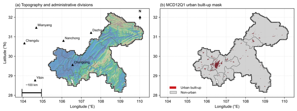
Chongqing lies in the eastern Sichuan Basin between 105.3–110.2° E and 28.2–32.2° N. The municipality covers 82,400 km2, the largest of China’s four province-level cities. Its resident population reached about 32 million in 2023, with two-thirds classed as urban. Figure 1a shows the terrain and the administrative divisions. Terrain in Figure 1a derives from the SRTM 30 m digital elevation model [32]. Administrative boundaries came from the official municipal shapefile.
Elevation rises from about 160 m along the Yangtze to over 2000 m in the southeast. Parallel ridges strike northeast to southwest and divide the west into valley corridors. The nine core districts occupy the valleys between the Zhongliang and Mingyue ranges. These districts hold the densest traffic and the main commercial functions. Regional centers, including Wanzhou, Fuling, Yongchuan, and Jiangjin, line the Yangtze and its tributaries. Heavy industry clusters at these river ports: chemicals at Fuling, materials and equipment at Wanzhou, and manufacturing at Yongchuan–Jiangjin. The northeastern and southeastern counties remain rural and forested, with low emission density.
The climate is humid subtropical with weak synoptic forcing. Annual mean wind speed stays near 1.5 m s−1, among the lowest for Chinese megacities [23]. Winter brings persistent stratus, fog, and temperature inversions under the basin’s stagnant high-humidity air. Summer convection deepens the boundary layer and speeds photochemical NO2 loss. These conditions favor wintertime pollutant accumulation. They also make the region a strict test case for emission controls. A control policy that works here should work in better-ventilated cities.
The emission structure differs between the core and the periphery. Transport dominates NOx in the nine core districts. The municipality registered over 6 million motor vehicles by 2023, most of them in the west. Industry dominates at the river-port centers, where chemical, materials, and equipment plants operate. Rural counties emit little NOx beyond towns, roads, and seasonal biomass burning, because sparse traffic and scattered combustion sources dominate there rather than concentrated industry. Vehicle-focused policies should register first in the core pixels. Industry-focused shifts should register at the ports and the receiving parks. Figure 1b displays the urban built-up mask used in the urban–rural analysis. Built-up pixels concentrate in the core districts, with secondary patches at the regional centers. Section 2.4 details the classification.

2.2. Data

2.2.1. TROPOMI NO2

Table 1 summarizes all datasets, their resolutions, and their roles in this study. We used the Sentinel-5P offline (OFFL) Level-3 tropospheric NO2 product hosted in GEE (COPERNICUS/S5P/OFFL/L3_NO2). The underlying Level-2 retrieval follows the KNMI algorithm. The algorithm fits NO2 slant columns in the 405–465 nm window, separates the stratospheric part, and converts to vertical columns with air-mass factors [33]. The GEE Level-3 product grids the Level-2 swaths after filtering out pixels with a quality flag below 0.75. This threshold removes cloud radiance fractions above 0.5, snow and ice scenes, and retrieval errors, following the product user guide [33]. The variable of interest is the tropospheric NO2 vertical column density in mol m−2. We converted all values to 1015 molecules cm−2, multiplying by 6.02214 × 10⁴. This unit eases comparison with the OMI and TROPOMI literature.
GEE grids the product at 0.01° and stores one image per orbit. Multiple orbits can cover the study area on one day at its latitude. Our compositing treats each orbit scene as one observation, the standard practice in GEE-based studies [20,31].
The record spans 1 January 2019 to 31 December 2024, six full calendar years. We excluded 2018 for two reasons. The OFFL processor version changed during 2018, and early data used a different along-track pixel size. The ground pixel shrank from 3.5 × 7 km to 3.5 × 5.5 km on 6 August 2019 [11]. This mid-2019 change affects pixel size, not calibration, and does not bias annual composites. TROPOMI crosses the equator near 13:30 local solar time. All composites therefore represent early-afternoon conditions. Afternoon columns run lower than morning columns because photolysis peaks at midday. Trend and contrast statements remain valid because the observation time is fixed.
Validation studies report a negative bias of 20–30% in TROPOMI tropospheric NO2 over polluted regions [33]. The bias stems from coarse a priori profiles and cloud treatment. It affects absolute levels more than relative patterns and trends. Our analysis rests on spatial contrasts, seasonal cycles, and trends. These quantities tolerate a stable systematic bias. We therefore report VCD values as observed and avoid absolute comparisons with surface standards.

2.2.2. MODIS Land Cover

We used the MODIS MCD12Q1 Collection 6.1 annual land-cover product at 500 m resolution [26]. The product classifies each cell with the IGBP scheme from a full year of surface reflectance. Class 13, urban and built-up lands, defines the urban class in this study. Reported overall accuracy for the IGBP layer is about 74%, with higher accuracy for the urban class in large cities [26]. The 2022 map served as the primary mask, near the midpoint of the study period. Maps for 2019 and 2023 supported a sensitivity test on urban expansion (Section 2.4).

2.2.3. ERA5 Meteorology

Monthly ERA5 reanalysis fields provided the meteorological context [34,35]. ERA5 is the fifth-generation ECMWF global reanalysis, supplied hourly at 0.25° resolution. We used the ERA5 hourly collection rather than ERA5-Land because the latter, being a land-surface product, does not carry boundary-layer height. We extracted boundary-layer height, 2 m temperature, and the 10 m wind components over the study area. Wind speed was computed as the scalar magnitude of the hourly u and v components before any temporal averaging, so that variable wind directions do not cancel and depress the mean. The hourly fields were then aggregated to the same 72 monthly steps as the NO2 composites and averaged over the municipality. Monthly anomalies were expressed relative to the six-year mean of the corresponding calendar month, which characterizes unusual months against their own climatology. Section 3.2 reports the resulting meteorological background and Section 4.2 uses the anomalies to test the 2021 high-NO2 episodes. We did not perform a formal meteorological normalization. Section 4.4 flags this as a limitation.

2.3. Compositing and Trend Analysis

All processing ran in GEE at a 5.5 km analysis grid, matching the native TROPOMI resolution. We resisted finer grids. Oversampling below the sensor footprint fabricates spatial detail without adding information. We built three composite sets from the daily Level-3 scenes. Monthly means covered the 72 months from January 2019 to December 2024. Seasonal means pooled all months of each season across the six years. Seasons follow the meteorological convention: MAM (March–April–May), JJA (June–July–August), SON (September–October–November), and DJF (December–January–February). Annual means covered each calendar year. Compositing used the arithmetic mean of all valid observations per pixel. Valid-scene counts vary through the year. Winter retains fewer scenes because cloud screening removes overcast days. Section 4.4 discusses the resulting sampling caveat.
Trends rest on the six annual composites. We estimated the slope at each pixel with the Theil–Sen method [27,35]. The estimator takes the median of the 15 pairwise slopes among the six annual values. Each pairwise slope divides the value difference by the year difference. The median makes the slope robust to single anomalous years, such as 2021. An ordinary least-squares fit would let that one year drag the whole slope.
The monthly series carried the sub-annual analysis. A 12-month centered running mean tracked the low-frequency evolution and suppressed the seasonal cycle. Monthly anomalies compared each month against the mean of the same calendar month across the six years. This anomaly form isolates unusual episodes, such as the 2020 lockdown and the 2021 peaks. Percentage changes cited in Section 3 use these same-month comparisons. Year-over-year forms avoid the seasonal aliasing that adjacent-month comparisons would introduce.
The annual (n = 6) Mann–Kendall test judged pixel significance [28]. With only six values, the test has limited power: its variance equals n(n − 1)(2n + 5)/18 = 28.33, and only strong monotonic changes reach the 5% level (|Z| ≥ 1.96). To strengthen the test for trends while preserving the seasonal structure, we additionally applied the Seasonal Mann–Kendall (SMK) test to the full 72-month series (2019-01 to 2024-12, period = 12) [36]. For each calendar month the series has six values; the seasonal S statistic sums the within-month S values and the variances add, so the effective sample is 72 months rather than six years. The seasonal Sen slope is the median of all within-month pairwise slopes. This raises the share of pixels flagged as significant from 2.3% (annual MK) to 42.6% (SMK). District-level statistics aggregated the pixel slopes and Z values by the 38 administrative units. Regional means used area weighting over all valid pixels.

2.4. Urban–Rural Classification

The urban–rural contrast required a mask at the NO2 grid scale. We aggregated the 500 m MCD12Q1 urban class to the 5.5 km grid. Each coarse cell contains about 121 fine cells. A grid cell counts as urban when built-up cover exceeds 50% of its area. All remaining cells count as non-urban. This majority rule avoids labeling a cell as urban from a single small town. It also dilutes the urban signal in mixed cells. True urban columns exceed the urban-cell average, so our contrast is conservative. The 2022 map defined the primary mask: 42 urban and 2985 non-urban cells. Recognizing that a 50% rule may exclude smaller satellite towns and fast-growing peripheries at 5.5 km resolution, we repeated the aggregation at 30% and 40% thresholds and checked whether the urban–rural contrast and convergence trend survived. The urban cell count rose from 42 (50%) to 58 (40%) and 76 (30%). Table S1 lists the per-threshold urban/rural means and the urban-to-rural ratio (U/R); the convergence direction was identical across all three thresholds, so the primary conclusion is not sensitive to the cut-off.
Urban extent grew during the study period. A fixed mask could bias the urban time series in either direction. Newly built areas would count as rural under an early mask. Pre-development fields would count as urban under a late mask. We repeated the urban aggregation with the 2019 and 2023 land-cover maps. The three masks produced near-identical urban annual means. Table S2 lists the sensitivity results, which are presented in Section 3.5. For the distribution analysis, we sampled up to 5000 cells per class from the multi-year mean field. Sampling avoids the double counting that full enumeration with overlapping grids can introduce. Box plots in Section 3.5 show the median, the interquartile range, and 1.5-IQR whiskers. Points beyond the whiskers appear as outliers. We report medians rather than means for the distributions. The urban class is small and right-skewed, and the median resists that skew. Annual class means, by contrast, use area-weighted averages over all class cells. The two statistics answer different questions: typical pixel level versus class total burden.
We also defined a convergence metric. The urban-to-rural ratio divides the urban annual mean by the non-urban annual mean. A falling ratio marks convergence between the two classes. Section 3.5 reports this ratio for each year.

2.5. Uncertainty Treatment

We handled four uncertainty sources by design rather than by correction. First, there is retrieval bias. The known 20–30% low bias in polluted scenes is systematic [24]. Contrasts, ratios, and trends cancel a stable multiplicative bias, so we restricted claims to these forms. Second, we perform sampling from cloud screening. We report the retained orbit count by season. Winter (DJF) retains 6.12 observations per pixel-month against 11.85 in summer (JJA); i.e., winter rests on 48% fewer scenes. Cloud-free winter days in the basin often coincide with stagnation and high NO2, so winter composites lean toward polluted conditions; we flag this and avoid gap filling, which would import assumptions the trend test could echo. Third, we consider test power. With six annual values, the Mann–Kendall test flags only strong changes. We paired the pixel test with the 72-month series, which carries more degrees of freedom. Fourth, we consider classification error. The urban mask mislabels some mixed cells at the 500 m source scale [26]. The three-year mask sensitivity test bounds this effect (Table S2). Together these choices trade completeness for defensibility. Every number in Section 3 survives a stable bias and a thin winter sample.

2.6. Workflow Summary

The full chain runs in six steps: Level-3 ingestion, quality screening, unit conversion, compositing, trend estimation, and zonal aggregation. Every step is executed server-side in GEE with the JavaScript API. We chose server-side execution in Google Earth Engine for three concrete reasons: first, feasibility: the compositing and pixel-wise trend computation run against the hosted archive, so no bulk download or local storage is needed and the local footprint stays at a few hundred megabytes of exports; second, co-location: GEE hosts the TROPOMI archive alongside the ERA5 meteorology and MODIS land cover used here, so the three are combined without reprojection or transfer overhead; third, reproducibility: any reader with a free account can rerun the scripts against the identical archive. The choice is one of tractability and reproducibility, not of approximation: the same statistics are computed as a local pipeline would. The scripts export composites as GeoTIFF and statistics as CSV for figure production. We drew the final figures with Matplotlib (version 3.7.1) and Cartopy (version 0.21.1) in Python (version 3.9). Map figures overlay the official vector boundary on the raster fields. Raster edges follow the 5.5 km grid, so the vector line defines the visual boundary. The complete GEE and Python code is available from the authors on request.

3. Results

3.1. Spatial Pattern of Tropospheric NO2

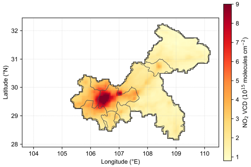
Figure 2 shows the mean tropospheric NO2 distribution over Chongqing during 2019–2024. NO2 VCD peaked in the central urban districts, exceeding 7 × 10¹⁵ molecules cm−2 around 106.5° E, 29.6° N. Levels declined outward along the Yangtze corridor toward Fuling and Wanzhou. The northeastern and southeastern mountainous counties stayed below 2 × 10¹⁵ molecules cm−2. The urban core therefore exceeded the remote counties by a factor of 3 to 4. To place these values in context, the Chongqing core maximum of 7 × 10¹⁵ molecules cm−2 is comparable to other large inland Chinese cities but remains below the 10–15 × 1015 molecules cm−2 reported from TROPOMI for the most polluted North China Plain conurbations, and it is of the same order as major European and North American metropolitan areas [15,16]. Chongqing is therefore a high-but-not-extreme case by international standards, which makes the internal contrasts examined here more informative than the absolute level. Section 4.1 develops this comparison. This gradient tracks the distribution of traffic, industry, and population in the valley city [17,37]. Secondary hotspots appeared over Wanzhou (108.4° E, 30.8° N) and the Yongchuan–Jiangjin industrial belt. Terrain shaped this pattern. The parallel ridge-and-valley system confines emissions within the valleys and limits ventilation [23]. The 5.5 km TROPOMI grid resolves these secondary features. OMI, at 13 × 24 km, merged them into one basin-wide blur in earlier studies [25,38].

3.2. Monthly Variation

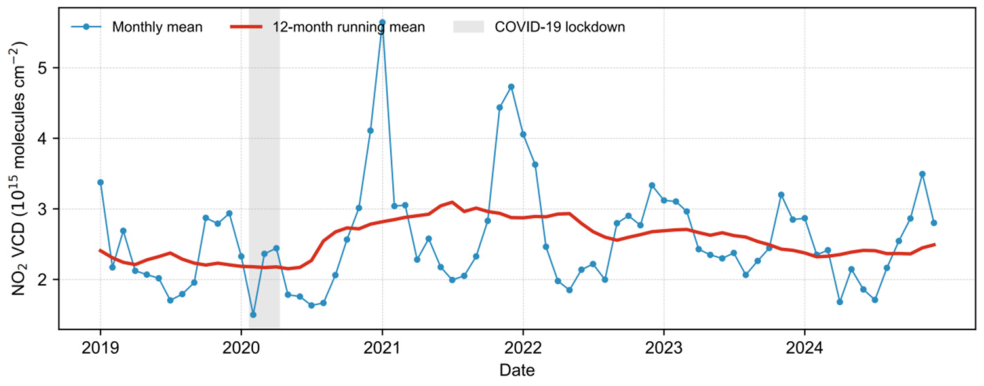
Figure 3 presents the monthly series of regional mean NO2 from January 2019 to December 2024. The regional monthly mean ranged from 1.5 to 5.6 × 10¹⁵ molecules cm−2. Each year showed a winter maximum and a summer minimum. Photochemical loss of NO2 shortens its lifetime in summer. Winter heating and a shallow boundary layer raise the columns [7]. The mean winter-to-summer ratio across the six years was about 1.6–1.7.
The meteorological background over the same period provides context for the NO2 record. We averaged the ERA5 hourly fields over the municipality and aggregated them to the same 72 months as the NO2 series. Ventilation in the basin is persistently weak. The six-year mean 10 m wind speed is 1.37 m s−1 and the six-year mean boundary-layer height is 340 m, both low by the standards of Chinese megacities and a direct consequence of the ridge-and-valley setting. Neither parameter drifts over the record. Annual mean wind speed stays within 1.32 to 1.46 m s−1 and annual mean boundary-layer height within 314 to 389 m, and both vary without direction: the shallowest year is 2021 and the deepest is 2022. Annual mean 2 m temperature, by contrast, rises from 15.9 to 17.1 °C, a warming of about 1.2 K that reflects regional climate rather than dispersion. The seasonal cycle is modest for the ventilation parameters. Winter (DJF) has the shallowest boundary layer at 299 m and the weakest winds at 1.29 m s−1, against 385 m and 1.41 m s−1 in summer (JJA), a seasonal contrast of only 29% in mixing depth. This is far too small to generate the winter-to-summer NO2 ratio of 1.6–1.7 reported above, which therefore rests mainly on the longer photochemical lifetime of NO2 in winter, with the shallower mixed layer as a secondary contributor. The stability of the ventilation parameters is itself informative. Because dispersion conditions show no multi-year drift, the 2019–2024 evolution of NO2 cannot be attributed to a systematic change in ventilation, which strengthens the emission-based reading of the record. We nonetheless refrain from a formal quantitative separation of the two influences (Section 4.2 and Section 4.4).
The lockdown in early 2020 cut the February value to 1.5 × 10¹⁵ molecules cm−2. This was the lowest month in the record, 31% below February 2019. March 2020 remained about 20% below March 2019, while April 2020 recovered to near the 2019 level as restrictions eased. Columns recovered to the pre-pandemic level by mid-2020.
January 2021 reached 5.6 × 10¹⁵ molecules cm−2, the highest month observed; this monthly peak exceeds the calendar-year means quoted later because it is a single-month value, not an annual average. This value was 1.8 times the January average of the other five years. December 2021 formed a second peak of 4.7 × 10¹⁵ molecules cm−2. Section 4.2 examines the meteorology behind these two episodes. After 2022 the running mean flattened near 2.4 × 10¹⁵ molecules cm−2. The 2024 annual mean retreated toward but remained above the 2019 level.

3.3. Seasonal Distribution

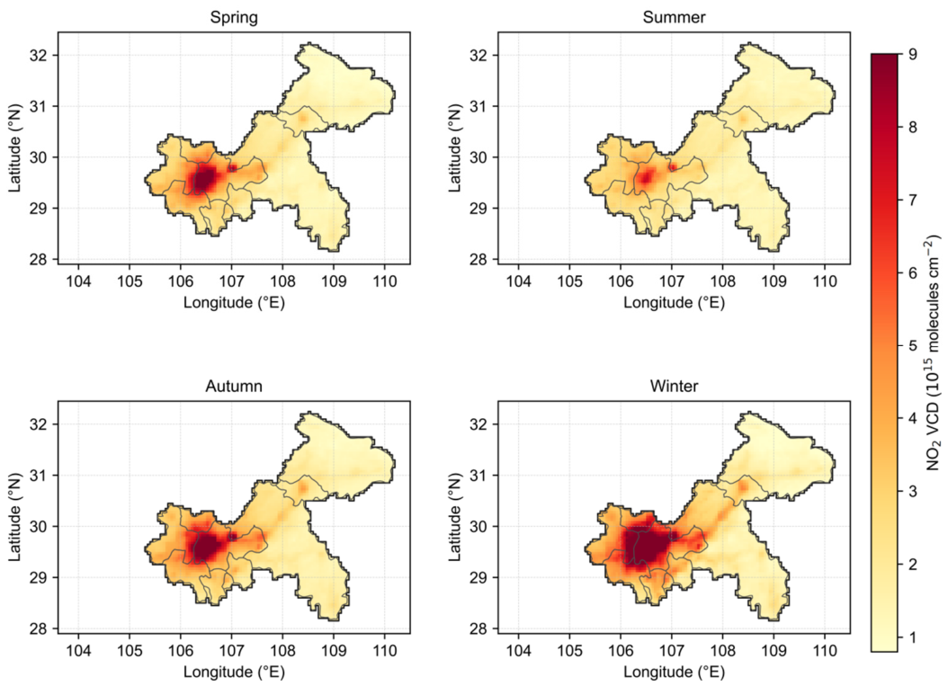
Figure 4 compares the four seasonal composites averaged over the six years. Winter columns were the highest and the most spatially extended. High values spread from the core across the western districts and along the Yangtze valley. Summer showed the weakest signal. The hotspot shrank to the central districts. Spring and autumn were transitional. Autumn exceeded spring over the western plain. Weaker convection and earlier heating demand explain the autumn excess.
Season also changed the shape of the polluted area, not only its level. The winter contour of 4 × 10¹⁵ molecules cm−2 enclosed roughly 6.3 times the summer area. In winter the Wanzhou hotspot connected to the core along the river valley. In summer the two separated. The seasonal amplitude in the urban core reached about a factor of 3. In the eastern counties the amplitude stayed below a factor of 2. Emission-dense areas thus dominate the seasonal cycle of the region.

3.4. Long-Term Trend

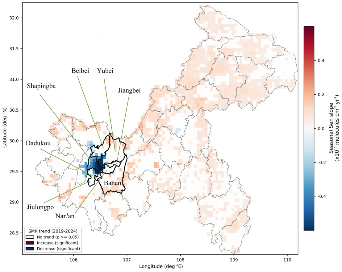
Figure 5 maps the pixel-wise Theil–Sen slope with Mann–Kendall significance for 2019–2024. Slopes ranged from −0.97 to +0.25 × 10¹⁵ molecules cm−2 yr−1 across the domain. Of 3308 valid pixels, 1409 (42.6%) showed a significant trend at p < 0.05, against only 2.3% under the six-year annual MK test; the SMK therefore recovers far more of the real structure. Table 2 lists the annual regional means behind these trends. The regional mean rose from 2019 to a maximum in 2021, then declined through 2022, re-bounded slightly in 2023 (+4.4%), and fell again in 2024. The area-weighted regional SMK Sen slope was +0.042 × 10¹⁵ molecules cm−2 yr−1 (Z = +1.46, p = 0.14), small and not significant. The near-zero regional trend is the average of opposite movements: strong core declines offset by widespread peripheral increases (Section 3.6). The trend sign, however, depended entirely on location. Urban pixels, by contrast, declined monotonically after 2021 (Section 3.5).

3.5. Urban–Rural Contrast

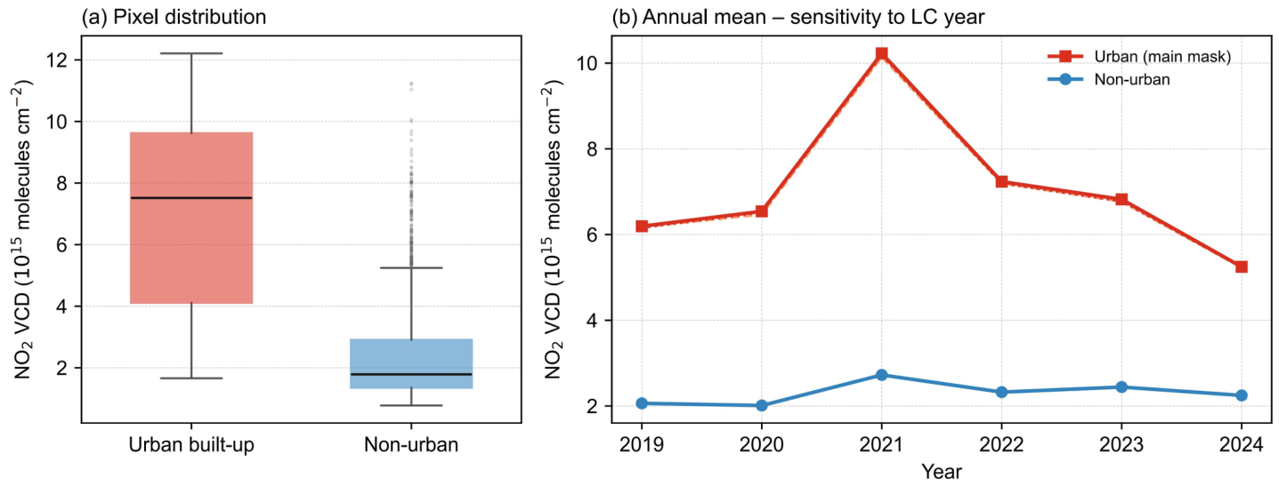
Figure 6 quantifies the contrast between built-up and non-urban pixels. Urban pixels averaged 7.0 × 10¹⁵ molecules cm−2 at the median, against 1.8 for non-urban pixels (Figure 6a). The interquartile ranges do not overlap. Urban annual means peaked at 10.2 × 10¹⁵ molecules cm−2 in 2021 and fell to 5.2 by 2024 (Figure 6b). This is a 49% drop from the peak. Non-urban means varied within 2.0 to 2.7 × 10¹⁵ molecules cm−2 and lacked a clear trend.
The urban-to-rural ratio traces the convergence year by year. The ratio stood at 3.0 in 2019, climbed to 3.8 in 2021, then narrowed to 2.3 in 2024. Urban decline drove the narrowing. Rural levels changed little over the same years. Masks from 2019, 2022, and 2023 land cover gave near-identical urban means (Figure 6b; Table S2). The mask year shifts the urban mean by under 1%. We further repeated the ratio at 30% and 40% built-up thresholds (76 and 58 urban cells, respectively). The urban–rural ratio fell from 2019 to 2024 at every threshold, so the convergence is robust to the choice of both land-cover year and built-up threshold (Table S1).

3.6. Core–Periphery Divergence in Trends

The trend map in Figure 5 splits Chongqing into two regimes. A contiguous cluster of negative slopes covers the nine core districts, with the strongest declines over the central districts that also hold the highest multi-year means. Under the SMK test, 29% of urban pixels decline significantly. The area-weighted core trend is negative (median urban Sen slope −0.11 × 10¹⁵ molecules cm−2 yr−1), confirming that the emission controls bite where traffic dominates.
The periphery moved the other way. Positive slopes dominate the northeastern counties around Wanzhou, Kaizhou, and Liangping, and a second patch follows the Yongchuan–Jiangjin belt in the southwest. Pixels with significant increases concentrate in these two areas (Figure 5). District-level SMK statistics show seven of the eight core districts with an area-weighted declining trend, against only 1 of 29 peripheral units.
The two regimes also differ in starting level. Declining pixels began high, mostly above 6 × 10¹⁵ molecules cm−2; rising pixels began low, mostly under 3 × 10¹⁵ molecules cm−2. High- and low-emission areas are converging toward the middle, consistent with the narrowing urban-to-rural ratio (Section 3.5). Chongqing therefore shows a “core down, periphery up” divergence rather than a uniform trend. Section 4.3 discusses the mechanisms and the policy consequences.

4. Discussion

4.1. Comparison with Previous Studies

Our spatial pattern agrees with OMI-based work on the Sichuan Basin for 2005–2016. That study placed the basin maximum over the Chengdu and Chongqing cores [23,25]. TROPOMI resolves structures that OMI blurred. The Wanzhou hotspot and the Yongchuan–Jiangjin belt emerge as separate features at 5.5 km resolution. The 2020 lockdown dip matches reductions of 30–50% reported for Chinese cities from TROPOMI [15,16]. Our regional decline after 2021 parallels the national NO2 decrease under 14th Five-Year Plan controls [39,40]. The urban decline, about 20% yr−1 relative to the anomalous 2021 peak (49% over three years), exceeds the typical post-2021 rates reported for eastern megacities [41], though the elevated 2021 baseline inflates this rate. Relative to 2019, urban columns in 2024 were about 15% lower, comparable to eastern-city reductions. Mountainous Chongqing thus kept pace with the flat coastal cities despite weaker ventilation.
The absolute level also merits comparison across megacities. Chongqing’s urban core, at a multi-year mean near 7 × 10¹⁵ molecules cm−2 and an urban annual mean of 5.2 × 10¹⁵ molecules cm−2 in 2024, sits in the upper-middle range of the global megacity distribution. It falls clearly below the Beijing–Tianjin–Hebei and Yangtze River Delta maxima, where TROPOMI columns exceed 10 × 1015 molecules cm−2 over the densest clusters [15,16], and it is broadly comparable to inland provincial capitals such as Chengdu and Xi’an [23,25]. Two considerations make this ranking noteworthy. First, Chongqing sustains these columns with a weaker emission density than the coastal clusters, because the basin ventilation is poor: a six-year mean wind speed of 1.37 m s−1 and a winter boundary layer of 299 m (Section 3.2) retain emissions that a coastal city would export. A given emission therefore yields a higher column here than on the plain, and the observed level overstates the underlying emission intensity relative to eastern cities. Second, the urban-to-rural ratio of 2.3 in 2024 is modest by megacity standards, reflecting both the genuine convergence documented in Section 3.5 and the large rural territory of a province-sized municipality. Chongqing is thus best characterized as a moderately polluted megacity whose burden is amplified by terrain rather than by exceptional emissions, which is precisely why the intra-city divergence, rather than the absolute level, carries the management message.

4.2. The 2021 High-NO2 Episodes

The two 2021 peaks deserve separate treatment. They dominate the interannual variability and set the reference point for the later decline. January 2021 reached 1.8 times the January norm (Section 3.2), and the ERA5 record allows us to test whether meteorology can account for it. It cannot. Boundary-layer height in January 2021 was 291 m against a January norm of 279 m, that is, 4.3% deeper than usual, and the 10 m wind speed was likewise 4.3% above its January norm. Dispersion conditions that month were therefore slightly better than average, not worse. The same holds, more weakly, for the second peak: December 2021 had a boundary layer 5.0% below its December norm and winds 2.4% below, anomalies that are unremarkable within a year whose largest monthly departures reach −30% (August) and −13% (May). Meteorology thus cannot explain either episode, and an emission-side explanation is required. National NOx emissions in early 2021 exceeded early-2020 levels as industry and transport rebounded from the 2020 restrictions [39,40], and the January peak coincides with that rebound. One caveat qualifies this reading rather than overturning it. Cloud screening thins the winter sample, and clear winter days in the basin tend to be the stagnant ones, so the monthly composite leans toward polluted days [42]. This sampling effect inflates winter columns generally; it cannot produce a 1.8-fold departure confined to a single January when the resolved meteorology of that month was, if anything, favorable to dispersion.
December 2021 repeated the pattern at 4.7 × 10¹⁵ molecules cm−2. Urban pixels felt both episodes harder than rural ones. The urban 2021 annual mean jumped 56% above 2020 (Figure 6b). The rural mean rose only 35%. This asymmetry is itself an emission signature: had a basin-wide meteorological anomaly driven the peaks, urban and rural columns would have risen more closely in proportion, whereas a rebound concentrated in traffic and industry raises the emission-dense valleys preferentially. The 2021 maximum is therefore best read as an emissions event.
We did not separate the two contributions quantitatively. Quantitative separation of meteorological and emission contributions is now standard practice in the literature, typically via meteorological normalization with random-forest or comparable models [43]. We did not apply such a correction here for two reasons. First, the six-year monthly record is short for training a stable normalization model at the pixel level, and the 2021 rebound is itself a compounded emissions-plus-weather event that such models struggle to attribute cleanly. Second, our conclusions rest on contrasts, ratios, and SMK trends that are robust to a stable multiplicative meteorological bias, so a normalization would not change the core divergence finding. We therefore flag this as a limitation (Section 4.4) and outline it as follow-up work. The qualitative reading stands either way. The 2021 maximum reflects rebound emissions meeting under near-normal dispersion conditions, so the peak signals emissions rather than weather. The subsequent decline toward pre-2021 levels confirms this reading.
The 2023 uptick of 4.4% above 2022 (Table 2) followed the final lifting of pandemic restrictions in early 2023 and the associated economic recovery, which raised traffic and industrial activity. ERA5 meteorology shows no basin-wide stagnation in 2023 comparable to the January 2021 episode, so the rebound is better explained by emission recovery than by anomalous weather. The renewed 2024 decline indicates the 2023 value was a transient post-pandemic bump rather than a reversal of the control-driven downward trend.

4.3. Interpreting the Core–Periphery Divergence

The divergence in Section 3.6 carries policy weight. Core districts cut NO2 while peripheral counties gained. Two mechanisms fit this pattern. Industrial relocation moved manufacturing from the core to district-level parks. Yongchuan, Fuling, and the northeastern counties received much of it [44]. The rising patches in Figure 5 match these receiving areas. County urbanization added a second push. Vehicle ownership and construction grew faster in the counties than in the saturated core during 2019–2024 [45]. Both mechanisms raise county NOx while the core sheds it.
The core decline has its own drivers. Chongqing enforced China VI vehicle standards from July 2019 [15,18,46]. Rail transit expanded through 2024 and displaced car trips in the central districts. New-energy vehicles took a growing share of urban traffic [45]. These measures target exactly the traffic-dominated core, which explains why the decline concentrates there.
A similar core-down, periphery-up structure appears in North China during 2019–2023 [20]. The pattern may therefore mark a general stage of Chinese urban development. Emission-intensive activity migrates outward while the core electrifies and de-industrializes. For management, the result argues against a core-only strategy. Peripheral counties need emission standards for the relocated industries now. Waiting lets their growth lock in higher baselines. The northeast cluster around Wanzhou deserves first attention. It combines significant upward trends with a growing secondary hotspot.

4.4. Uncertainties and Limitations

Four caveats apply. First, TROPOMI measures the tropospheric column, not surface concentration. Column-to-surface ratios vary with boundary-layer depth. Seasonal comparisons therefore carry extra uncertainty [42]. Second, cloud screening removes many winter scenes over the basin. We quantified this directly: retained orbit counts fall from 11.85 observations per pixel-month in summer (JJA) to 6.12 in winter (DJF); i.e., winter composites rest on 48% fewer scenes and favor clear, stagnant, high-NO2 days. Section 4.2 discusses how this affects the 2021 peaks. The bias is acknowledged rather than corrected. Third, six annual values limit the power of the annual Mann–Kendall test; we therefore based Figure 5 on the 72-month seasonal MK test, which recovers 42.6% significant pixels. Fourth, our urban mask uses a 50% built-up threshold at the 5.5 km grid. Mixed pixels dilute the urban signal. The true urban–rural contrast likely exceeds our estimate, but the convergence conclusion is robust across 30–50% thresholds (Table S1). Fifth, we did not perform a meteorological normalization. The urban–rural contrast and the SMK trends are presented as observed column quantities. We note that the ERA5 ventilation parameters show no multi-year drift across 2019–2024 (Section 3.2), so no systematic meteorological trend is being carried into our trend estimates; a random-forest normalization would nonetheless refine the month-to-month attribution and is left to follow-up given the short record, as noted in Section 4.2.

5. Conclusions

We analyzed tropospheric NO2 over Chongqing for 2019–2024 using TROPOMI observations processed in Google Earth Engine. Four findings stand out. First, NO2 concentrates in the central districts and along the Yangtze valley. The core exceeds the mountainous counties by a factor of 3 to 4. TROPOMI resolves the Wanzhou and Yongchuan–Jiangjin hotspots as separate features. Second, the record divides into three phases. The 2020 lockdown produced the minimum, 31% below the prior February. Rebound emissions produced the 2021 maximum under near-normal dispersion conditions, so the peak reflects emissions rather than weather. Thereafter the regional mean stabilized: the area-weighted seasonal Mann–Kendall slope of +0.042 × 10¹⁵ molecules cm−2 yr−1 is not significant (p = 0.14), because core declines and peripheral increases cancel in the average. Third, urban built-up pixels fell 49% from the 2021 peak. Non-urban pixels showed no clear trend. The urban-to-rural ratio narrowed from its 2021 peak of 3.8 to 2.3 in 2024 (3.0 in 2019). The contrast is robust to the land-cover mask year. Fourth, trends diverge in space. The core districts declined while most peripheral counties rose. Significant increases cluster around Wanzhou and the southwestern industrial belt. Industrial relocation and county urbanization explain the rise. The divergence carries a management message. Core-focused controls worked, but emissions are shifting to the periphery. Extending vehicle and industrial standards to the receiving counties should come next. Follow-up work should normalize the series for meteorology and attach surface NO2 estimates to the column record.

Supplementary Materials

The following supporting information can be downloaded at https://www.mdpi.com/article/10.3390/atmos17080791/s1, Table S1: Sensitivity to the built-up fraction threshold (30%, 40%, 50%); Table S2: Sensitivity of urban annual mean NO2 (1015 molecules cm−2) to the land-cover mask year (2019, 2022, 2023).

Author Contributions

Conceptualization, K.C.; methodology, Z.L. and K.C.; software, Z.L.; validation, K.C.; formal analysis, K.C.; investigation, Z.L.; resources, P.Z.; data curation, P.Z.; writing—original draft preparation, Z.L.; writing—review and editing, K.C.; visualization, Z.L.; supervision, K.C.; project administration, K.C.; funding acquisition, K.C. All authors have read and agreed to the published version of the manuscript.

Funding

This work was funded by the National Natural Science Foundation of China (Grant No. 42230604 and 42475092).

Institutional Review Board Statement

Not applicable.

Informed Consent Statement

Not applicable.

Data Availability Statement

The Sentinel-5P TROPOMI NO2 data are publicly available in Google Earth Engine (COPERNICUS/S5P/OFFL/L3_NO2). MODIS MCD12Q1 land-cover data are available from the NASA LP DAAC, and ERA5 data from the Copernicus Climate Data Store. The derived composites, statistics, and processing scripts are available from the corresponding author upon reasonable request.

Acknowledgments

We thank the European Space Agency and the Copernicus programme for providing the Sentinel-5P TROPOMI data, the Royal Netherlands Meteorological Institute (KNMI) for the NO2 retrieval algorithm, NASA LP DAAC for the MODIS land-cover product, and the European Centre for Medium-Range Weather Forecasts (ECMWF) for the ERA5 reanalysis. The Google Earth Engine platform provided the cloud-computing resources for this study.

Conflicts of Interest

The authors declare no conflicts of interest.

Abbreviations

The following abbreviations are used in this manuscript:
NO2Nitrogen Dioxide
VCDVertical Column Density
NOxNitrogen Oxides
TROPOMITROPOspheric Monitoring Instrument
GEEGoogle Earth Engine
LCLand-Cover Class
MAMMarch, April, May
JJAJune, July, August
SONSeptember, October, November
DJFDecember, January, February

References

  1. Crutzen, P.J. The role of NO and NO2 in the chemistry of the troposphere and stratosphere. Annu. Rev. 1979, 7, 443–472. [Google Scholar] [CrossRef] [Scilit]
  2. Seinfeld, J.H. Urban air pollution: State of the science. Science 1989, 243, 745–752. [Google Scholar] [CrossRef] [Scilit] [PubMed]
  3. Seinfeld, J.H.; Pandis, S.N. Atmospheric Chemistry and Physics: From Air Pollution to Climate Change; John Wiley & Sons: Hoboken, NJ, USA, 2016. [Google Scholar]
  4. Griffith, S.M.; Huang, X.H.; Louie, P.; Yu, J.Z. Characterizing the thermodynamic and chemical composition factors controlling PM2.5 nitrate: Insights gained from two years of online measurements in Hong Kong. Atmos. Environ. 2015, 122, 864–875. [Google Scholar] [CrossRef] [Scilit]
  5. Achakulwisut, P.; Brauer, M.; Hystad, P.; Anenberg, S.C. Global, national, and urban burdens of paediatric asthma incidence attributable to ambient NO2 pollution: Estimates from global datasets. Lancet Planet. Health 2019, 3, e166–e178. [Google Scholar] [CrossRef] [Scilit] [PubMed]
  6. Naidoo, R.N. NO2 increases the risk for childhood asthma: A global concern. Lancet Planet. Health 2019, 3, e155–e156. [Google Scholar] [CrossRef] [Scilit] [PubMed]
  7. Shah, V.; Jacob, D.J.; Li, K.; Silvern, R.F.; Zhai, S.; Liu, M.; Lin, J.; Zhang, Q. Effect of changing NOx lifetime on the seasonality and long-term trends of satellite-observed tropospheric NO2 columns over China. Atmos. Chem. Phys. 2020, 20, 1483–1495. [Google Scholar] [CrossRef] [Scilit]
  8. Beirle, S.; Platt, U.; Wenig, M.; Wagner, T. Weekly cycle of NO2 by GOME measurements: A signature of anthropogenic sources. Atmos. Chem. Phys. 2003, 3, 2225–2232. [Google Scholar] [CrossRef] [Scilit]
  9. Duncan, B.N.; Lamsal, L.N.; Thompson, A.M.; Yoshida, Y.; Lu, Z.; Streets, D.G.; Hurwitz, M.M.; Pickering, K.E. A space-based, high-resolution view of notable changes in urban NOx pollution around the world (2005–2014). J. Geophys. Res. Atmos. 2016, 121, 976–996. [Google Scholar] [CrossRef] [Scilit]
  10. Burrows, J.P.; Weber, M.; Buchwitz, M.; Rozanov, V.; Ladstätter-Weißenmayer, A.; Richter, A.; DeBeek, R.; Hoogen, R.; Bramstedt, K.; Eichmann, K.-U. The global ozone monitoring experiment (GOME): Mission concept and first scientific results. J. Atmos. Sci. 1999, 56, 151–175. [Google Scholar] [CrossRef]
  11. Veefkind, J.P.; Aben, I.; McMullan, K.; Förster, H.; De Vries, J.; Otter, G.; Claas, J.; Eskes, H.; De Haan, J.; Kleipool, Q. TROPOMI on the ESA Sentinel-5 Precursor: A GMES mission for global observations of the atmospheric composition for climate, air quality and ozone layer applications. Remote Sens. Environ. 2012, 120, 70–83. [Google Scholar] [CrossRef] [Scilit]
  12. Tang, D.; Zhan, Y.; Yang, F. A review of machine learning for modeling air quality: Overlooked but important issues. Atmos. Res. 2024, 300, 107261. [Google Scholar] [CrossRef] [Scilit]
  13. Beirle, S.; Borger, C.; Dörner, S.; Li, A.; Hu, Z.; Liu, F.; Wang, Y.; Wagner, T. Pinpointing nitrogen oxide emissions from space. Sci. Adv. 2019, 5, eaax9800. [Google Scholar] [CrossRef] [Scilit] [PubMed]
  14. Goldberg, D.L.; Lu, Z.; Streets, D.G.; de Foy, B.; Griffin, D.; McLinden, C.A.; Lamsal, L.N.; Krotkov, N.A.; Eskes, H. Enhanced Capabilities of TROPOMI NO2: Estimating NOx from North American Cities and Power Plants. Environ. Sci. Technol. 2019, 53, 12594–12601. [Google Scholar] [CrossRef] [Scilit] [PubMed]
  15. Liu, F.; Page, A.; Strode, S.A.; Yoshida, Y.; Choi, S.; Zheng, B.; Lamsal, L.N.; Li, C.; Krotkov, N.A.; Eskes, H. Abrupt decline in tropospheric nitrogen dioxide over China after the outbreak of COVID-19. Sci. Adv. 2020, 6, eabc2992. [Google Scholar] [CrossRef] [Scilit] [PubMed]
  16. Bauwens, M.; Compernolle, S.; Stavrakou, T.; Müller, J.F.; Van Gent, J.; Eskes, H.; Levelt, P.F.; Van Der A, R.; Veefkind, J.; Vlietinck, J. Impact of coronavirus outbreak on NO2 pollution assessed using TROPOMI and OMI observations. Geophys. Res. Lett. 2020, 47, e2020GL087978. [Google Scholar] [CrossRef] [Scilit] [PubMed]
  17. Zheng, B.; Tong, D.; Li, M.; Liu, F.; Hong, C.; Geng, G.; Li, H.; Li, X.; Peng, L.; Qi, J. Trends in China’s anthropogenic emissions since 2010 as the consequence of clean air actions. Atmos. Chem. Phys. 2018, 18, 14095–14111. [Google Scholar] [CrossRef] [Scilit]
  18. Xie, Y.; Rodríguez, F. Zero-Emission Integration in Heavy-Duty Vehicle Regulations: A Global Review and Lessons for China; The International Council on Clean Transportation: Washington, DC, USA, 2021. [Google Scholar]
  19. Automotive Data of China Co., Ltd. Analysis of Low-Carbon Transformation Pathways of Automotive Industry for Carbon Neutrality. In China Automotive Low Carbon Action Plan (2022) Low Carbon Development Strategy and Transformation Path for Carbon Neutral Automotive; Springer: Berlin/Heidelberg, Germany, 2023; pp. 115–222. [Google Scholar]
  20. Li, L.; Wang, Y.; Zhang, Y.; Chen, D. Spatiotemporal Variability and Associated Environmental Factors of Tropospheric NO2 Column Density over North China from TROPOMI Observations, 2019–2023. Remote Sens. 2026, 18, 1758. [Google Scholar] [CrossRef] [Scilit]
  21. Xue, R.; Wang, S.; Zhang, S.; He, S.; Liu, J.; Tanvir, A.; Zhou, B. Estimating city NOx emissions from TROPOMI high spatial resolution observations—A case study on Yangtze River Delta, China. Urban Clim. 2022, 43, 101150. [Google Scholar] [CrossRef] [Scilit]
  22. Wei, Q.; Song, W.; Dai, B.; Wu, H.; Zuo, X.; Wang, J.; Chen, J.; Li, J.; Li, S.; Chen, Z. Spatiotemporal estimation of surface NO2 concentrations in the Pearl River Delta region based on TROPOMI data and machine learning. Atmos. Pollut. Res. 2025, 16, 102353. [Google Scholar] [CrossRef] [Scilit]
  23. Ning, G.; Wang, S.; Yim, S.H.L.; Li, J.; Hu, Y.; Shang, Z.; Wang, J.; Wang, J. Impact of low-pressure systems on winter heavy air pollution in the northwest Sichuan Basin, China. Atmos. Chem. Phys. 2018, 18, 13601–13615. [Google Scholar] [CrossRef] [Scilit]
  24. Verhoelst, T.; Compernolle, S.; Pinardi, G.; Lambert, J.-C.; Eskes, H.J.; Eichmann, K.-U.; Fjæraa, A.M.; Granville, J.; Niemeijer, S.; Cede, A. Ground-based validation of the Copernicus Sentinel-5p TROPOMI NO2 measurements with the NDACC ZSL-DOAS, MAX-DOAS and Pandonia global networks. Atmos. Meas. Tech. 2021, 14, 481–510. [Google Scholar] [CrossRef] [Scilit]
  25. Wu, K.; Wang, Y.; Qiao, Y.; Liu, Y.; Wang, S.; Yang, X.; Wang, H.; Lu, Y.; Zhang, X.; Lei, Y. Drivers of 2013–2020 ozone trends in the Sichuan Basin, China: Impacts of meteorology and precursor emission changes. Environ. Pollut. 2022, 300, 118914. [Google Scholar] [CrossRef] [Scilit] [PubMed]
  26. Friedl, M.; Sulla-Menashe, D. MCD12Q1 MODIS/Terra Aqua Land Cover Type Yearly L3 Global 500m SIN Grid V006; NASA EOSDIS Land Processes Distributed Active Archive Center: Sioux Falls, SD, USA, 2019.
  27. Theil, H. A rank-invariant method of linear and polynomial regression analysis. Indag. Math. 1950, 12, 173. [Google Scholar]
  28. Mann, H.B. Nonparametric tests against trend. Econom. J. Econom. Soc. 1945, 13, 245–259. [Google Scholar] [CrossRef] [Scilit]
  29. Gorelick, N.; Hancher, M.; Dixon, M.; Ilyushchenko, S.; Thau, D.; Moore, R. Google Earth Engine: Planetary-scale geospatial analysis for everyone. Remote Sens. Environ. 2017, 202, 18–27. [Google Scholar] [CrossRef] [Scilit]
  30. Rabiei-Dastjerdi, H.; Mohammadi, S.; Saber, M.; Amini, S.; McArdle, G. Spatiotemporal Analysis of NO2 Production Using TROPOMI Time-Series Images and Google Earth Engine in a Middle Eastern Country. Remote Sens. 2022, 14, 1725. [Google Scholar] [CrossRef] [Scilit]
  31. Sameh, S.; Zarzoura, F.; El-Mewafi, M. Spatio-temporal Analysis Mapping of Air Quality Monitoring in Cairo using Sentinel-5 satellite data and Google earth engine. Mansoura Eng. J. 2023, 49, 3. [Google Scholar] [CrossRef] [Scilit]
  32. Farr, T.G.; Rosen, P.A.; Caro, E.; Crippen, R.; Duren, R.; Hensley, S.; Kobrick, M.; Paller, M.; Rodriguez, E.; Roth, L. The shuttle radar topography mission. Rev. Geophys. 2007, 45, RG2004. [Google Scholar] [CrossRef] [Scilit]
  33. Van Geffen, J.; Boersma, K.; Van Roozendael, M.; Hendrick, F.; Mahieu, E.; De Smedt, I.; Sneep, M.; Veefkind, J. Improved spectral fitting of nitrogen dioxide from OMI in the 405–465 nm window. Atmos. Meas. Tech. 2015, 8, 1685–1699. [Google Scholar] [CrossRef] [Scilit]
  34. Hersbach, H.; Bell, B.; Berrisford, P.; Hirahara, S.; Horanyi, A.; Munoz-Sabater, J.; Nicolas, J.; Peubey, C.; Radu, R.; Schepers, D.; et al. The ERA5 global reanalysis. Q. J. R. Meteorol. Soc. 2020, 146, 1999–2049. [Google Scholar] [CrossRef] [Scilit]
  35. Sen, P.K. Estimates of the regression coefficient based on Kendall’s tau. J. Am. Stat. Assoc. 1968, 63, 1379–1389. [Google Scholar] [CrossRef]
  36. Hirsch, R.M.; Slack, J.R.; Smith, R.A. Techniques of trend analysis for monthly water quality data. Water Resour. Res. 1982, 18, 107–121. [Google Scholar] [CrossRef] [Scilit]
  37. Li, H.; Zheng, B.; Lei, Y.; Hauglustaine, D.; Chen, C.; Lin, X.; Zhang, Y.; Zhang, Q.; He, K. Trends and drivers of anthropogenic NOx emissions in China since 2020. Environ. Sci. Ecotechnol. 2024, 21, 100425. [Google Scholar] [CrossRef] [Scilit] [PubMed]
  38. Huang, R.; Ju, T.; Dong, H.; Duan, J.; Fan, J.; Liang, Z.; Geng, T. Analysis of atmospheric SO2 in Sichuan-Chongqing region based on OMI data. Environ. Monit. Assess. 2021, 193, 849. [Google Scholar] [CrossRef] [Scilit] [PubMed]
  39. Chen, L.; Cai, Z.; Liu, Y.; Sun, K.; Yang, D.; Wang, X.; Wang, Y. Satellite data-driven estimates of NOx and coemitted CO2 from coal-fired power plants in China (2021–2024). Environ. Res. Lett. 2026, 21, 144001. [Google Scholar] [CrossRef] [Scilit]
  40. Wang, W.; Li, B.; Chen, B. Improved surface NO2 Retrieval: Double-layer machine learning model construction and spatio-temporal characterization analysis in China (2018–2023). J. Environ. Manag. 2025, 384, 125439. [Google Scholar] [CrossRef] [Scilit] [PubMed]
  41. Zhao, Z.; Lu, Y.; Zhan, Y.; Cheng, Y.; Yang, F.; Brook, J.R.; He, K. Long-term spatiotemporal variations in surface NO2 for Beijing reconstructed from surface data and satellite retrievals. Sci. Total Environ. 2023, 904, 166693. [Google Scholar] [CrossRef] [Scilit] [PubMed]
  42. Lamsal, L.N.; Martin, R.V.; van Donkelaar, A.; Steinbacher, M.; Celarier, E.A.; Bucsela, E.; Dunlea, E.J.; Pinto, J.P. Ground-level nitrogen dioxide concentrations inferred from the satellite-borne Ozone Monitoring Instrument. J. Geophys. Res.-Atmos. 2008, 113, D16308. [Google Scholar] [CrossRef] [Scilit]
  43. Grange, S.K.; Carslaw, D.C. Using meteorological normalisation to detect interventions in air quality time series. Sci. Total Environ. 2019, 653, 578–588. [Google Scholar] [CrossRef] [Scilit] [PubMed]
  44. Wang, H.; Kong, X.; Luo, J.; Li, P.; Chen, X.; Xie, T. An approach to urban system spatial planning in Chengdu Chongqing economic circle using geospatial big data. Front. Earth Sci. 2023, 11, 1252597. [Google Scholar] [CrossRef] [Scilit]
  45. Song, X.; Hao, Y.; Zhu, X. Air pollutant emissions from vehicles and their abatement scenarios: A case study of Chengdu-Chongqing Urban Agglomeration, China. Sustainability 2019, 11, 6503. [Google Scholar] [CrossRef] [Scilit]
  46. Tang, G.; Wang, S.; Du, B.; Cui, L.; Huang, Y.; Xiao, W. Study on pollutant emission characteristics of different types of diesel vehicles during actual road cold start. Sci. Total Environ. 2022, 823, 153598. [Google Scholar] [CrossRef] [Scilit] [PubMed]
Figure 1. (a) Study area with terrain, administrative boundaries, and major urban centers. The inset marks the location within China. (b) Urban built-up area from MODIS MCD12Q1 land cover (2022, IGBP class 13).
Atmosphere 17 00791 g001
Figure 2. Mean tropospheric NO2 vertical column density over Chongqing during 2019–2024.
Atmosphere 17 00791 g002
Figure 3. Monthly variation in regional mean tropospheric NO2 over Chongqing, 2019–2024. The red line shows the 12-month running mean. The gray band marks the COVID-19 lockdown (23 January to 8 April 2020).
Atmosphere 17 00791 g003
Figure 4. Seasonal mean tropospheric NO2 over Chongqing averaged for 2019–2024: spring (MAM), summer (JJA), autumn (SON), and winter (DJF).
Atmosphere 17 00791 g004
Figure 5. Pixel–wise seasonal Mann–Kendall Sen slope of tropospheric NO2 over Chongqing for the 72–month series (2019–2024, period = 12). The color scale spans −0.6 to +0.6 × 10¹⁵ molecules cm−2 yr−1; full–color pixels are significant (p < 0.05), faint pixels are not. Bold outlines mark the nine core districts.
Atmosphere 17 00791 g005
Figure 6. Urban–rural contrast in tropospheric NO2. (a) Distribution of pixel values for urban built-up and non-urban classes, 2019–2024 mean. (b) Annual means by land type. Dashed and dotted lines show urban means from the 2019 and 2023 land-cover masks. LC = land-cover class; LC 2019 and LC 2023 denote the MCD12Q1 land-cover product year used to define the urban mask.
Atmosphere 17 00791 g006
Table 1. Datasets used in this study, with sources, spatial and temporal resolutions, periods, and usage.
DatasetSource/GEE IDSpatial ResolutionTemporal ResolutionPeriod
Tropospheric NO2 VCDSentinel-5P TROPOMI,3.5 × 5.5 km (since August 2019)DailyJanuary 2019–December 2024
Land coverMODIS MCD12Q1 (IGBP),500 mAnnual2022
Meteorological fieldsERA5 (ECMWF)0.25°Hourly
(aggregated to monthly)
January 2019–December 2024
Administrative boundary Chongqing municipal boundaryVector--
Table 2. Annual mean tropospheric NO2 VCD over Chongqing, 2019–2024.
YearAnnual_mean_no2Annual_changeAnnual_change_pct
20192.1496
20202.1073−0.0422−1.97
20212.88350.776236.83
20222.4279−0.4556−15.8
20232.53480.10684.4
20242.3077−0.2271−8.96
Disclaimer/Publisher’s Note: The statements, opinions and data contained in all publications are solely those of the individual author(s) and contributor(s) and not of MDPI and/or the editor(s). MDPI and/or the editor(s) disclaim responsibility for any injury to people or property resulting from any ideas, methods, instructions or products referred to in the content.