Article

WaveDiff-R: Wavelet-Guided Diffusion Network with Residual Sub-Band Enhancement for Remote Sensing Dehazing

1
School of Information Engineering, Chuzhou Polytechnic, Chuzhou 239000, China
2
College of Computer and Information Science, Southwest University, Chongqing 400715, China
*
Author to whom correspondence should be addressed.
Atmosphere 2026, 17(7), 684; https://doi.org/10.3390/atmos17070684
Submission received: 9 June 2026 / Revised: 4 July 2026 / Accepted: 7 July 2026 / Published: 12 July 2026
(This article belongs to the Section Atmospheric Techniques, Instruments, and Modeling)

Abstract

Atmospheric haze is a major source of image degradation in Earth observation systems, reducing visibility, distorting spectral information, and obscuring surface details in remote sensing imagery. Physics-based dehazing methods often hinge on simplified atmospheric assumptions, whereas purely data-driven networks struggle with ultra-high-resolution overhead imagery and the wide spatial variability of haze. To address these challenges in a way that respects the characteristics of very large remote sensing scenes, we introduce WaveDiff-R, a wavelet-guided diffusion framework with residual sub-band enhancement. Rather than running diffusion directly in the full spatial domain, WaveDiff-R performs a multi-level discrete wavelet transform (DWT) to separate low- and high-frequency components in a geometry-aware manner. The wavelet-guided diffusion module (WGDM) performs conditional diffusion only on the low-frequency approximation coefficients A K after a K-level DWT, reducing the denoising target by 4 K while restoring global luminance and chromaticity. In parallel, the residual sub-band enhancement module (RSEM), built with residual state space blocks (RSSBs), refines the high-frequency sub-bands, recovering sharp edges and textures by jointly modeling long-range dependencies and local details. This collaborative design couples global consistency with fine-grained fidelity while maintaining an efficiency suitable for real-world remote sensing pipelines. Extensive experiments on six benchmark datasets covering synthetic and real scenarios showed that WaveDiff-R achieved consistently strong results, surpassing state-of-the-art natural-image and remote sensing dehazing baselines in both quantitative metrics and visual quality.

1. Introduction

Haze is pervasive during remote sensing image acquisition; it refers specifically to aerosol- and droplet-driven scattering and absorption of light [1]. In satellite and aerial imagery typical of ultra-high-resolution mapping, the immediate consequences are a diminished visibility, lowered contrast, and pronounced color cast, which blur land-cover boundaries and suppress fine textures. Such degradation undermines both human interpretation and the reliability of downstream automation, notably land-use classification [2] and object detection [3,4]. Under the atmospheric scattering model adopted here, haze perturbs not only direct object transmission, but also the airlight term, yielding spatially non-uniform, scene-dependent corruption that standard, one-size-fits-all corrections fail to capture.
Traditional remote sensing dehazing approaches are largely built on physically grounded priors [1]—including the dark channel prior (DCP) [5], haze-lines [6], and non-local regularities [7]—to estimate the transmission map and atmospheric light before inverting the scattering model. While typically lightweight and fast, these pipelines hinge on assumptions that can break under complex terrain or heterogeneous aerosol distributions common in operational imagery. In particular, DCP-style methods are prone to failure over intrinsically bright surfaces (e.g., deserts, snowfields, metal or concrete rooftops), which frequently appear in satellite and aerial scenes, leading to biased transmission estimates and color artifacts. Learning-based methods have recently gained traction in remote sensing image restoration, leveraging convolutional neural networks (CNNs) [8], transformers [9], and physics-guided deep architectures [10] to directly learn the mapping from degraded to haze-free images. Supervised approaches can produce high-quality results when trained on paired data, but such datasets are rare in remote sensing due to the difficulty of acquiring the same scene under both hazy and clear conditions. Synthetic datasets based on radiative transfer models can partially address this gap, yet domain shifts between simulated and real-world conditions often impair generalization. Unsupervised and semi-supervised approaches [11,12] reduce the dependency on paired labels, but can suffer from color shifts, the loss of fine structures, or over-smoothing, especially for large-format, high-resolution satellite data.
Recently, diffusion models (DMs) [13] have emerged as a new paradigm for image generation and restoration, offering a high perceptual quality and strong robustness against mode collapse. In restoration tasks, DMs progressively reverse a noise-adding process to recover the target image [14,15,16,17], and have been explored for weather-related degradation removal [18,19]. However, the direct application of DMs to remote sensing dehazing faces two key obstacles: 1. Computational burden: Remote sensing imagery is often ultra-high-resolution (e.g., 4K), making iterative denoising in the full spatial domain prohibitively slow and memory-intensive. 2. Content stability: The reverse process starts from randomly sampled Gaussian noise; even under conditional guidance, this randomness can introduce geometric inconsistency or hallucinated structures, which are unacceptable for quantitative remote sensing analyses. These challenges call for a computationally efficient, yet detail-preserving, diffusion framework tailored to the characteristics of remote sensing imagery.
Motivated by an initial observation (see Figure 1), we identified a key insight into the frequency characteristics of haze degradation in remote sensing imagery: the low-frequency components are severely affected by atmospheric scattering, leading to global brightness attenuation and color distortion, whereas the high-frequency components largely preserve structural cues, but suffer from edge blurring and texture suppression. Further, by exchanging the low- and high-frequency sub-bands between clear and hazy images, we verified the complementary roles of these components in perceptual restoration. Specifically, replacing the low-frequency sub-band of a hazy image with that from a clear image markedly improves the overall contrast and color fidelity. This phenomenon indicates that an effective dehazing strategy should jointly restore the global low-frequency appearance and enhance high-frequency details. To this end, we propose WaveDiff-R, a wavelet-guided conditional diffusion network with residual sub-band enhancement designed for efficient and faithful remote sensing image dehazing. WaveDiff-R consists of two key components: the wavelet-guided diffusion model (WGDM) and the residual sub-band enhancement module (RSEM). Unlike conventional diffusion models operating in the full spatial domain, the WGDM applies a multi-level two-dimensional discrete wavelet transform (2D-DWT) to decompose the hazy input and performs conditional diffusion only on the compact low-frequency coefficients, which encapsulate the most haze-affected global luminance and chromatic information. This frequency-selective design reduces the spatial size of the denoising target by 4 K times, substantially lowering the computational cost while preserving the essential scene structure. Meanwhile, the RSEM focuses on enhancing the high-frequency sub-bands that contain texture and edge information. It employs a lightweight, yet powerful, refinement mechanism based on the residual state space block (RSSB), where the vision state space module (VSSM) captures long-range dependencies, and depthwise convolutions model local structural patterns. This targeted enhancement restores haze-suppressed fine details without introducing geometric or spectral hallucinations, which is crucial for quantitative remote sensing analyses. By integrating the WGDM and RSEM, WaveDiff-R achieves the synergistic restoration of the global appearance and local details, delivering a state-of-the-art performance on both synthetic and real-world remote sensing dehazing benchmarks.
Our main contributions are summarized as follows:
  • We propose WaveDiff-R, a wavelet-guided conditional diffusion framework that selectively performs denoising in the low-frequency domain, dramatically reducing the computational cost for ultra-high-resolution remote sensing imagery.
  • We propose the wavelet-guided diffusion model (WGDM), which performs conditional diffusion only on compact low-frequency coefficients, reducing the computation while preserving the essential global appearance.
  • We introduce the residual sub-band enhancement module (RSEM), which leverages residual state space modeling to refine high-frequency sub-bands, effectively restoring fine textures and edges without hallucinations.
  • Extensive experiments on multiple synthetic and real-world datasets demonstrated that WaveDiff-R achieved a superior quantitative accuracy and perceptual quality compared to existing state-of-the-art remote sensing dehazing methods.

2. Related Works

2.1. Natural Image Single-Image Dehazing

Early single-image dehazing follows a physically grounded image-formation view—most notably the atmospheric scattering model (ASM)—that treats haze as the joint effect of scene-radiance attenuation and airlight contamination. A hazy measurement (I(x)) can be written as:
I ( x ) = J ( x ) t ( x ) + A 1 t ( x ) ,
where ( J ( x ) ) is the latent clear radiance, ( t ( x ) ) denotes the medium transmission (often parameterized as ( t ( x ) = exp β d ( x ) ) with scattering coefficient ( β ) and path length (d)), and ( A ) is the global atmospheric light. Estimating ( J ( x ) ) from ( I ( x ) ) is ill-posed without additional constraints because both ( t ( x ) ) and ( A ) are unknown.
To regularize the inversion, a series of handcrafted priors have been proposed. The dark-channel prior (DCP) [5] leverages the empirical tendency of haze-free outdoor patches to contain a near-zero intensity in at least one channel, yielding a proxy for transmission. Haze-lines [6] exploit linear color structures in RGB space to couple transmission and airlight estimation. The color attenuation prior (CAP) [7] introduces depth cues via brightness–saturation attenuation, and boundary-constrained or edge-aware smoothness terms help preserve salient transitions. Non-local formulations further utilize long-range self-similarity to maintain structural coherence. These priors are interpretable and computationally light, making them attractive for large collections and real-time scenarios. However, the underlying assumptions frequently clash with overhead remote sensing imagery. High-albedo, homogeneous regions—deserts, snowfields, salt flats, rooftops, and sunglint-affected waters—violate the dark-channel assumption, biasing transmission and inducing color shifts.
Deep learning moved dehazing beyond hand-crafted priors to data-driven restoration. Early progress was led by CNNs, but the field has steadily shifted toward models with stronger long-range context. DehazeFormer [20] combines local convolution with global self-attention, and MITNet [21] promotes cross-talk between clean and hazy branches to recover structure. A parallel line of work is frequency-aware—FSDGN and PhDNet [8,22] operate on spectral components to rebuild high-frequency detail suppressed by scattering. Efficiency-oriented designs (e.g., DEA-Net [9]) and generalist frameworks (OneRestore [10]) further extend the scope across multiple degradations. Yet most of these systems are trained on natural-image corpora with synthetic haze. When transferred to remote sensing, the domain gap becomes evident: semantic cues that help at ground level (object outlines, horizon lines) are weak or absent in nadir or near-nadir imagery, and many architectures give insufficient attention to spectral fidelity and radiometric stability—properties that are essential for geospatial analyses.

2.2. Remote Sensing Single-Image Dehazing

Remote sensing image dehazing (RSID) has grown its own toolbox to cope with the modality’s particularities—orthographic projection, scene-scale and heterogeneous haze, weak semantic cues, and multi-band constraints. Unpaired adversarial pipelines such as MO-GAN and Dehaze-AGGAN [11,12] sidestep the scarcity of paired clean targets. Physics-guided designs, exemplified by GPD-Net [23], embed scattering priors to improve the robustness under real atmospheric conditions. Multi-scale and attention mechanisms—for example, UAV-specific double-scale transmission optimization [24] and SFAN [25]—seek to separate global haze removal from fine-detail reconstruction. More recently, diffusion-based frameworks (ARDD-Net [26]) and progressive refinement networks (PSR-Net [27]) have advanced the state of the art, showing a stronger adaptability across a range of haze densities. Despite this progress, RSID still wrestles with a three-way trade-off among physical interpretability, detail preservation, and computational efficiency. These limitations motivate hybrid strategies that fuse explicit, physically informed priors with modern generative modeling, aiming for band-consistent, radiometrically stable restoration while maintaining a throughput suitable for large-area remote sensing workflows.

2.3. Diffusion Models for Image Restoration

Diffusion-based generative models, typified by DDPMs [13], learn the reverse of a gradual noising process: iterative denoising maps Gaussian noise to images. This schedule preserves high-frequency detail and yields a strong perceptual quality. Building on this idea, IDDPM [28] uses conditional guidance for super-resolution, RePaint [16] introduces iterative resampling for inpainting, and IR-SDE [29] formulates the dynamics in continuous time. Extensions include cold diffusion [14], which adapts the corruption–denoising pair to non-standard degradations, and variational treatments [18] that make inferences more tractable for inverse problems.
Despite this progress, many diffusion-based restorers [19] remain largely data-driven and seldom encode task physics. In dehazing, constraints from the atmospheric scattering model—e.g., the transmission or illumination structure—are rarely enforced, which can cause instability or structural drift under spatially varying haze. These issues are amplified in remote sensing by large-scale, heterogeneous atmospheric effects.
Recent studies have also explored the combination of wavelet transform and diffusion models. Song et al. [30] proposed WGDNet for single-pixel imaging, where an initial reconstruction is decomposed into low- and high-frequency components. The low-frequency component is enhanced by adaptive diffusion, while the high-frequency component is directionally refined by a multi-frequency adaptive fusion attention (MAFA) mechanism, followed by residual spatial adaptive fusion. Li et al. [31] proposed a hierarchical wavelet diffusion model, in which multi-scale wavelet representations are mainly used as conditional information to guide the diffusion process. These methods demonstrate that wavelet-domain priors can improve diffusion-based reconstruction and restoration. However, their frequency usage is different from ours. WGDNet relies on attention-based high-frequency fusion, while HWDM mainly introduces wavelet features as diffusion conditions. In contrast, WaveDiff-R explicitly decouples the restoration mechanisms of different frequency components: conditional diffusion is restricted to the low-frequency approximation coefficient A K , whereas the high-frequency sub-bands are preserved and refined by residual state space modeling. This design reduces the diffusion sampling burden and strengthens long-range structural modeling in high-frequency details.

3. Preliminaries

3.1. Conditional Diffusion Models

Diffusion models [13] describe a data distribution by simulating a two-stage stochastic process: a destruction phase that gradually converts a clean signal into noise, and a reconstruction phase that learns to reverse this transformation. The forward phase is fixed and injects Gaussian perturbations in small increments, while the reverse phase is parameterized by a neural network that predicts how to remove noise step-by-step. In conditional variants, additional observations are introduced to bias the reconstruction toward a specific target, which is particularly useful in image restoration tasks such as remote sensing dehazing.
Forward diffusion. Let x 0 be a haze-free image. The forward process generates latent states x 1 , , x T according to:
q ( x t x t 1 ) = N ( 1 β t x t 1 , β t I ) ,
where β t is a variance schedule controlling the noise increment at each step. Chaining these transitions yields:
q ( x 1 : T x 0 ) = t = 1 T q ( x t x t 1 ) ,
and as t approaches T, the distribution converges to standard Gaussian noise. This process also admits a closed-form sampling path from x 0 to any x t :
q ( x t x 0 ) = N α ¯ t x 0 , ( 1 α ¯ t ) I ,
where α t = 1 β t and α ¯ t = s = 1 t α s .
Reverse denoising with conditioning. The generative phase starts from pure noise x T N ( 0 , I ) and sequentially produces cleaner samples. In the conditional case, a degraded image y is provided as guidance. The reverse transition is defined as:
p θ ( x t 1 x t , y ) = N μ θ ( x t , t , y ) , Σ θ ( x t , t ) ,
where the network ϵ θ implicitly parameterizes μ θ by predicting the noise component injected during the forward process.
Learning objective. Training is commonly formulated as a noise regression task:
L = E x 0 , y , t , ϵ ϵ ϵ θ ( x t , t , y ) 2 2 ,
where x t is obtained by a forward perturbation of x 0 . The clean estimate at step t can be recovered via:
x ^ 0 = x t 1 α ¯ t ϵ θ ( x t , t , y ) α ¯ t .
Iterating from t = T to t = 0 produces a haze-free reconstruction aligned with the conditioning input.

3.2. Discrete Wavelet Transformation

Let I [ m , n ] be a discrete image of size H × W with c channels, and let ϕ ( t ) and ψ ( t ) denote the scaling (low-pass) and wavelet (high-pass) functions, respectively. The 1D discrete wavelet transform (DWT) [32] of a discrete signal x [ k ] is defined by:
a j + 1 [ p ] = k Z h [ k 2 p ] a j [ k ] ,
d j + 1 [ p ] = k Z g [ k 2 p ] a j [ k ] ,
where a j and d j denote the approximation and detail coefficients at scale j, h [ k ] and g [ k ] are the discrete low-pass and high-pass filter coefficients, and 2 p represents dyadic downsampling by a factor of two.
For the Haar wavelet [33], the filters are:
h = 1 2 [ 1 , 1 ] , g = 1 2 [ 1 , 1 ] .
The 2D-DWT applies the 1D DWT separably along the rows and columns. Given I [ m , n ] , the four sub-bands at scale j + 1 are:
A [ m , n ] = m n h [ m 2 m ] h [ n 2 n ] I [ m , n ] ,
V [ m , n ] = m n h [ m 2 m ] g [ n 2 n ] I [ m , n ] ,
H [ m , n ] = m n g [ m 2 m ] h [ n 2 n ] I [ m , n ] ,
D [ m , n ] = m n g [ m 2 m ] g [ n 2 n ] I [ m , n ] ,
where A is the approximation (low–low) sub-band containing the low-frequency structure, V is the vertical detail (low–high) sub-band, H is the horizontal detail (high–low) sub-band, and D is the diagonal detail (high–high) sub-band.
In matrix form, Equations (11)–(14) can be expressed as:
{ A , V , H , D } = 2 D-DWT ( I ) = { ( I L r L c ) 2 , ( I L r H c ) 2 , ( I H r L c ) 2 , ( I H r H c ) 2 } ,
where L r , L c , H r , H c are low/high-pass filters applied along rows (r) and columns (c), and 2 denotes downsampling by 2 in both spatial dimensions.
For a multi-scale decomposition with depth K, the approximation coefficient is recursively decomposed:
{ A k , V k , H k , D k } = 2 D-DWT ( A k 1 ) , A 0 = I .
After K levels, A K has its spatial resolution reduced by 4 K relative to the original image.
In the context of remote sensing image dehazing, A encapsulates global illumination and coarse structural information, which is most affected by atmospheric scattering, while { V , H c , D } retain fine edges and textures, but suffer from contrast loss. This separation provides a natural foundation for designing frequency-selective restoration pipelines, such as guiding diffusion processes primarily on A while enhancing { V , H c , D } through dedicated detail refinement modules.

4. Methodology

4.1. Overview

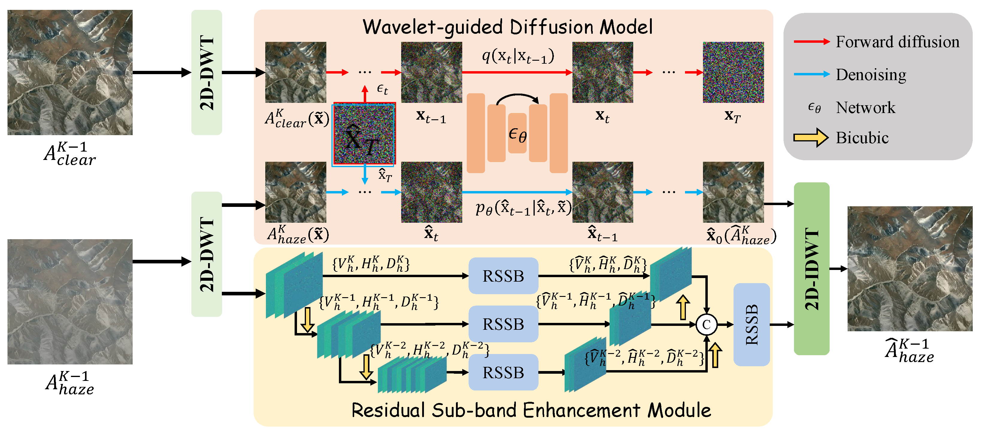
The proposed WaveDiff-R framework addresses the challenges of efficient and detail-preserving remote sensing image dehazing by leveraging a wavelet-guided conditional diffusion process coupled with residual sub-band enhancement. As illustrated in Figure 2, the hazy input image is first decomposed into low- and high-frequency sub-bands through a multi-level 2D-DWT. This decomposition reveals that haze primarily distorts the low-frequency approximation coefficients, which encode global luminance and color information, while the high-frequency detail coefficients retain structural contours, but suffer from a reduced contrast and edge blurring.
Based on this observation, WaveDiff-R comprises two synergistic components: (1) the wavelet-guided diffusion model (WGDM), which performs the conditional diffusion process exclusively on the compact low-frequency coefficients to restore global appearance with a significantly reduced computational cost, and (2) the residual sub-band enhancement module (RSEM), which refines the high-frequency detail coefficients using a lightweight, but effective, residual state space block (RSSB) to recover sharp textures and edges without introducing hallucinated structures.

4.2. Wavelet-Guided Diffusion Model

Unlike conventional conditional diffusion models that operate directly in the full spatial domain, the WGDM restricts the denoising process to the compact low-frequency representation obtained from multi-level 2D-DWT decomposition. This design is motivated by two observations from our frequency analysis (Figure 1): (1) haze degradation in remote sensing imagery primarily corrupts the low-frequency component, leading to global luminance attenuation and color bias; (2) high-frequency sub-bands retain most structural contours, but require only lightweight enhancement, making full-domain iterative denoising computationally wasteful.
Formally, given the decomposition
{ A K , H K } = DWT K ( I ) , H K = { V k , H k , D k } k = 1 K ,
we denote A clear K as the low-frequency coefficients of a haze-free image and A low K as those from its hazy counterpart. The WGDM learns to restore A clear K from A low K via a conditional diffusion process, avoiding unnecessary high-frequency iterations.
The forward noising process for A clear K is defined as:
q ( x t | x t 1 ) = N x t ; 1 β t x t 1 , β t I ,
with x 0 = A clear K and a fixed variance schedule { β t } t = 1 T . By closed-form reparameterization:
q ( x t | x 0 ) = N α ¯ t x 0 , ( 1 α ¯ t ) I ,
where α t = 1 β t and α ¯ t = s = 1 t α s .
The reverse process is conditioned on x ˜ = A low K :
p θ ( x t 1 | x t , x ˜ ) = N x t 1 ; μ θ ( x t , t , x ˜ ) , Σ θ ( x t , t ) .
The training objective minimizes the error in the noise prediction:
L WGDM = E A clear K , A haze K , t , ϵ ϵ ϵ θ ( x t , t , x ˜ ) 2 2 .
We clarify that the computational load mainly refers to the high memory and sampling cost caused by performing iterative denoising in the full-resolution image space. WaveDiff-R addresses this issue by decomposing the input image with a K-level DWT and applying the WGDM only to the low-frequency approximation coefficients A K . Since the spatial size of A K is reduced by 4 K , the diffusion target becomes much more compact, which substantially reduces the cost of iterative sampling.

4.3. Residual Sub-Band Enhancement Module

While the WGDM effectively restores the global luminance and color in the low-frequency component A haze K , haze-induced degradation in remote sensing imagery also manifests in the high-frequency sub-bands H K = { V haze k , H haze k , D haze k } k = 1 K , where edges and fine textures suffer from blurring and contrast suppression. These details are critical for quantitative remote sensing tasks, such as building extraction or road network mapping, and require targeted enhancement without introducing geometric artifacts.
To address this, we introduced the residual sub-band enhancement module (RSEM), which progressively refines high-frequency details from multiple wavelet decomposition levels. As shown in Figure 2, the enhancement proceeds in a top-down manner: starting from the highest decomposition level K, each set of high-frequency sub-bands is processed by a residual state space block (RSSB), which models both global and local dependencies. The refined features are then upsampled and fused with the corresponding sub-bands at the next lower level, allowing information to flow across scales.
Formally, for the k-th decomposition level ( k [ 1 , K ] ), let H h k = { V h k , H h k , D h k } be the high-frequency coefficients. The RSEM enhancement can be described as:
H ^ h k = RSSB H h k + 2 H ^ h k + 1 ,
where 2 ( · ) denotes bicubic upsampling by a factor of 2, and H ^ h k + 1 is the refined high-frequency set from the next coarser scale. At the coarsest level K, only the original coefficients are processed:
H ^ h K = RSSB ( H h K ) .
After enhancement, the refined high-frequency components { H ^ h k } are recombined with the restored low-frequency component A ^ K via the inverse wavelet transform (IDWT), yielding the final haze-free image. This multi-scale refinement ensures that structural fidelity is maintained while effectively restoring the local contrast lost due to atmospheric scattering.

4.4. Residual State Space Block

State space models (SSMs) have recently emerged as an efficient alternative to self-attention for modeling long-range dependencies with O ( H W ) complexity. In particular, the visual state space model (VSSM) extends the 1D selective scan mechanism of S6 [34] to the 2D image domain by performing horizontal and vertical state transitions. Compared with convolutional layers, the VSSM can capture global spatial correlations beyond the local receptive field, which is essential for restoring large-scale structures degraded by haze. Compared with vision transformers, it avoids the quadratic complexity of attention, making it more scalable to ultra-high-resolution remote sensing images. These properties are particularly advantageous for remote sensing dehazing, where the haze distribution is spatially non-uniform and long-range structural dependencies are crucial for preserving the scene geometry.
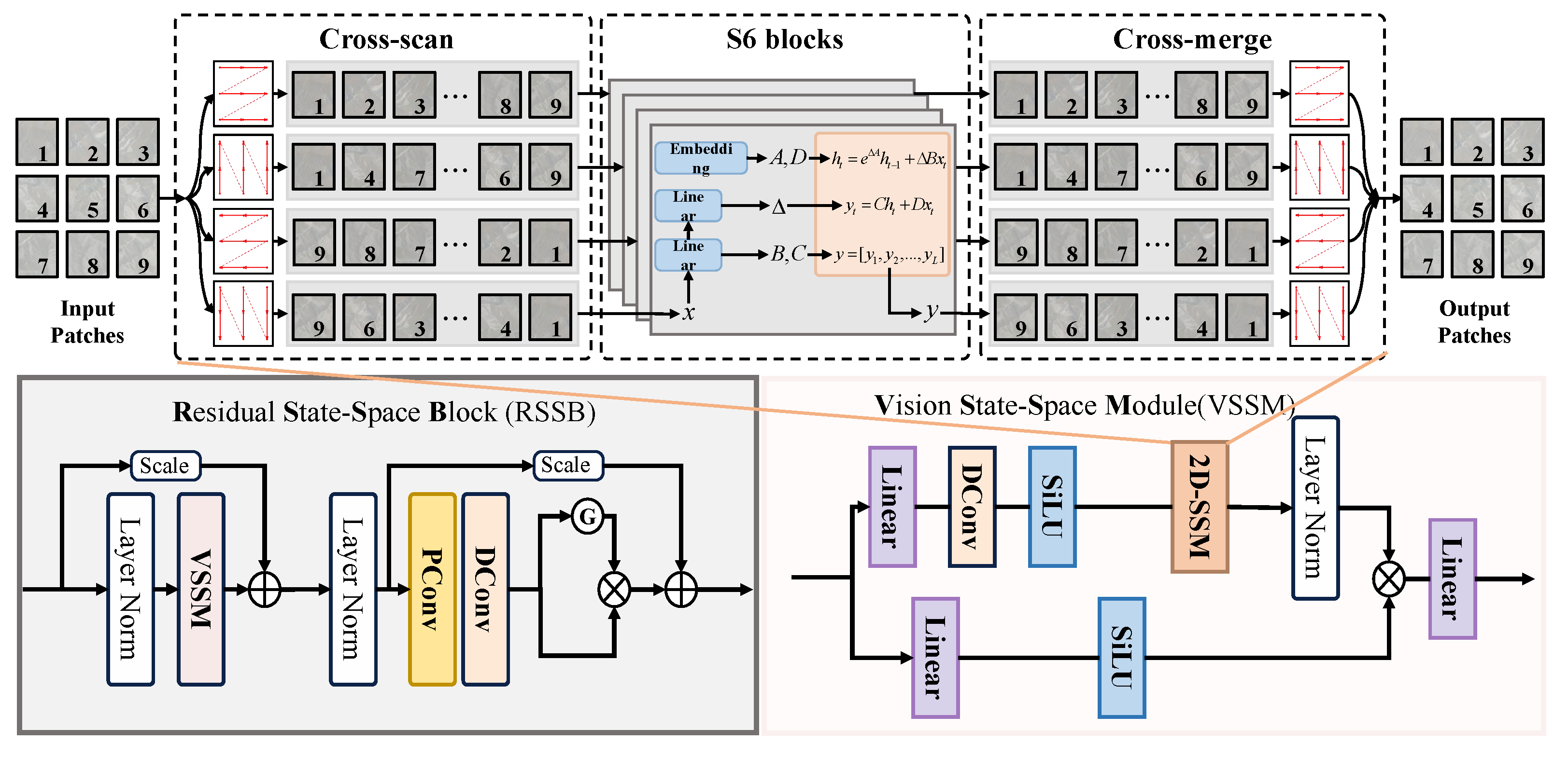
As shown in Figure 3, the residual state space block (RSSB) serves as the fundamental refinement unit in the residual sub-band enhancement module (RSEM), focusing on restoring the high-frequency sub-bands { V h k , H h k , D h k } obtained from the k-th level 2D-DWT decomposition. These vertical, horizontal, and diagonal detail coefficients are concatenated along the channel dimension to form the input tensor F in k R C × H × W , where C denotes the number of channels per sub-band. The RSSB first applies layer normalization and processes the normalized feature through the VSSM to model global dependencies:
F g k = VSSM ϕ LN ( F in k ) .
In parallel, a local branch applies layer normalization, a pointwise convolution ϕ PConv , and a depthwise convolution ϕ DConv to enhance fine-grained structures:
F l k = ϕ DConv ( ϕ PConv ( ϕ LN ( F in k ) ) ) .
The two branches are fused by element-wise multiplication, followed by a scaling parameter γ and a residual connection:
F out k = F in k + γ · F g k F l k .
This design ensures that both large-scale structural corrections and local texture restorations are jointly optimized.
Visual State Space Module (VSSM). Within the RSSB, the VSSM is responsible for global context modeling. Given an input X R C × H × W , the VSSM first applies two parallel linear projections:
Q = ϕ Linear 1 ( X ) , K = ϕ Linear 2 ( X ) ,
where ϕ Linear 1 and ϕ Linear 2 are linear layers.
The K branch is refined using depthwise convolution followed by SiLU activation:
K = SiLU ϕ DConv ( K ) .
As shown in Figure 3, by following [34], the 2D-SSM module performs horizontal and vertical state transitions to capture long-range dependencies across the spatial dimensions:
G = 2 D-SSM ( K ) .
The outputs of the two branches are combined via element-wise multiplication:
Y = Q G .
Finally, Y is normalized and projected back to the original channel dimension:
F global = ϕ Linear 3 ϕ LN ( Y ) .
By embedding the VSSM into the RSSB, our design effectively merges the global spatial context with local texture enhancement, enabling the accurate and geometry-preserving restoration of high-frequency sub-bands in remote sensing dehazing.

4.5. Total Training Objectives

The proposed WaveDiff-R is optimized in two complementary stages. First, the wavelet-guided diffusion model (WGDM) is trained to restore the low-frequency average coefficient A low K at the coarsest scale, as described in Section 4.2, where the corresponding loss L WGDM has been defined.
Second, the residual sub-band enhancement module (RSEM) refines the high-frequency detail coefficients { V ^ k , H ^ k , D ^ k } k = 1 K , which are then combined with the WGDM-restored low-frequency component A ^ K via an inverse discrete wavelet transform (IDWT) to produce the final reconstructed image:
I ^ rec = IDWT { A ^ k , V ^ k , H ^ k , D ^ k } k = 1 K .
Given the ground-truth clean image I gt , the reconstruction loss is formulated as:
L rec = μ 1 · L 1 I ^ rec , I gt + μ 2 · L FFT I ^ rec , I gt + μ 3 · 1 SSIM I ^ rec , I gt ,
where L 1 is the pixel-wise L1 loss, L FFT enforces frequency-domain consistency, and SSIM preserves structural similarity.
Finally, the total objective for end-to-end optimization is:
L total = L WGDM + L rec .
This joint training scheme ensures that the WGDM captures the global low-frequency structure, while the RSEM recovers fine-grained high-frequency details, resulting in visually coherent and geometrically consistent restored images.
DDIM-based efficient sampling. During training, the WGDM learns the standard noise prediction function over the full diffusion time range. During inference, we employed DDIM sampling to obtain an accelerated deterministic reverse trajectory. Let ( τ S , τ S 1 , , τ 0 ) be a shortened timestep sequence selected from the original diffusion process, where S T . In our work, we adopted a 10-step sampling strategy (i.e., S = 10 ) for efficient inference. Let c = A haze K denote the hazy low-frequency condition. Given the current noisy low-frequency coefficient x τ s , the predicted clean coefficient is computed as
x ^ 0 = x τ s 1 α ¯ τ s ϵ θ ( x τ s , τ s , c ) α ¯ τ s .
With the stochastic variance term removed, the deterministic DDIM update from τ s to τ s 1 is given by
x τ s 1 = α ¯ τ s 1 x ^ 0 + 1 α ¯ τ s 1 ϵ θ ( x τ s , τ s , c ) .
This formulation allows the reverse process to skip many intermediate DDPM steps while maintaining a stable restoration trajectory.

5. Experiments

5.1. Datasets

To ensure a thorough and fair assessment of WaveDiff-R under diverse haze conditions and scene types, we conducted experiments on six widely-used remote sensing dehazing benchmarks, covering both synthetic and real-world scenarios:
SateHaze1K [35]: A synthetic dataset with three haze-level subsets (thin, moderate, and thick), each containing 400 paired images. Following common practice, we adopted a 320/35/45 split for training, validation, and testing, respectively. RSID [36]: An authentic remote sensing dehazing dataset containing 1000 hazy–clean pairs. We randomly selected 900 images for training and 100 for testing, ensuring no scene overlap between the splits. LHID and DHID [37]: Two synthetic datasets distinguished by haze density: a light-haze image dataset (LHID), with 14,490 training and 500 testing pairs, and a dense-haze image dataset (DHID), with 30,517 training and 500 testing pairs. These datasets allow for a controlled evaluation across varying atmospheric opacity levels. RICE [38]: Derived from Google Earth imagery, this dataset covers diverse landscapes such as urban areas, deserts, mountains, and oceans. It is divided into two subsets: RICE1, with 402 training and 98 testing images, and RICE2, with 590 training and 146 testing images. RRSD300 [39]: A collection of 300 real-world aerial images affected by haze, sourced from Microsoft Bing and the DIOR dataset. It reflects the complex, uncontrolled atmospheric conditions encountered in practical remote sensing applications.

5.2. Quantitative Comparison

Table 1 reports the quantitative results of WaveDiff-R and recent state-of-the-art dehazing approaches, including both natural scene image (NSI) methods [8,9,10,20,21,22,40,41,42] and remote sensing image (RSI) methods [25,36,37,43,44,45,46,47], on five benchmark datasets.
First, our WaveDiff-R consistently achieved the best overall performance across all datasets. DHID (dense haze): WaveDiff-R reached 29.313 dB/0.947 SSIM. Against the best NSI method, OneRestore [10], this is + 0.539 dB ( + 1.87 % ) PSNR and + 0.008 ( + 0.85 % ) SSIM. Compared with the best RSI baseline SFAN [25] (29.173/0.942), the gains were + 0.140 dB ( + 0.48 % ) and + 0.005 ( + 0.53 % ).
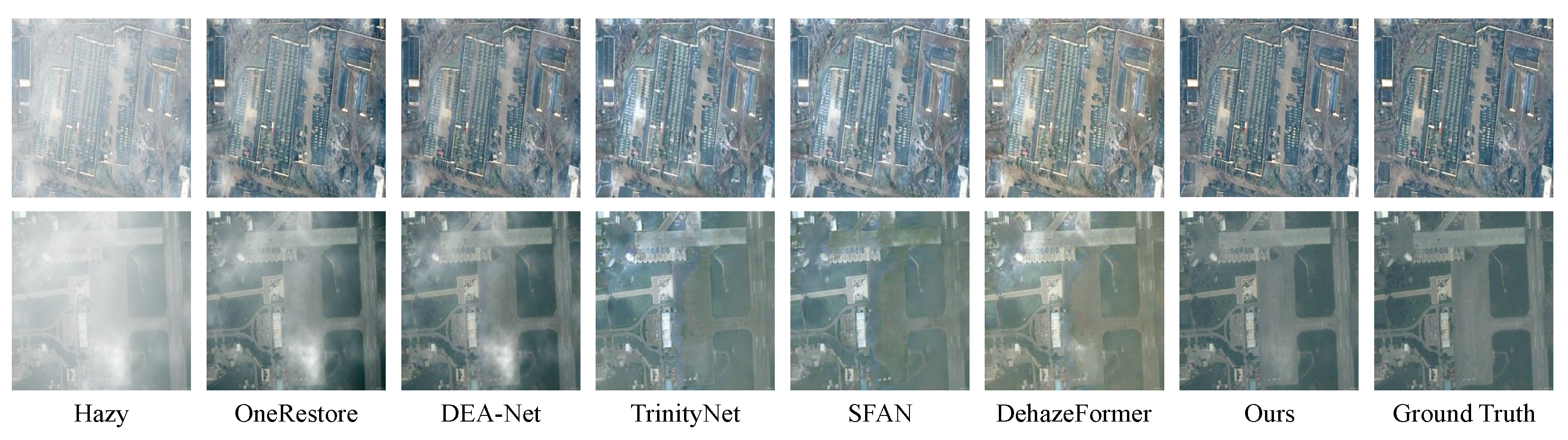
LHID (light haze): Light haze favors subtle enhancement without over-restoration. Our model reported 34.174 dB/0.973, improving on OneRestore (33.951/0.966) by + 0.223 dB and + 0.007 SSIM, and slightly surpassing SFAN (34.029/0.970) by + 0.145 dB and + 0.003 SSIM. We attribute the margins to the RSEM’s residual sub-band refinement, which sharpens contours and edge transitions without halos. See Figure 4 for visual comparisons of the global contrast and local detail.
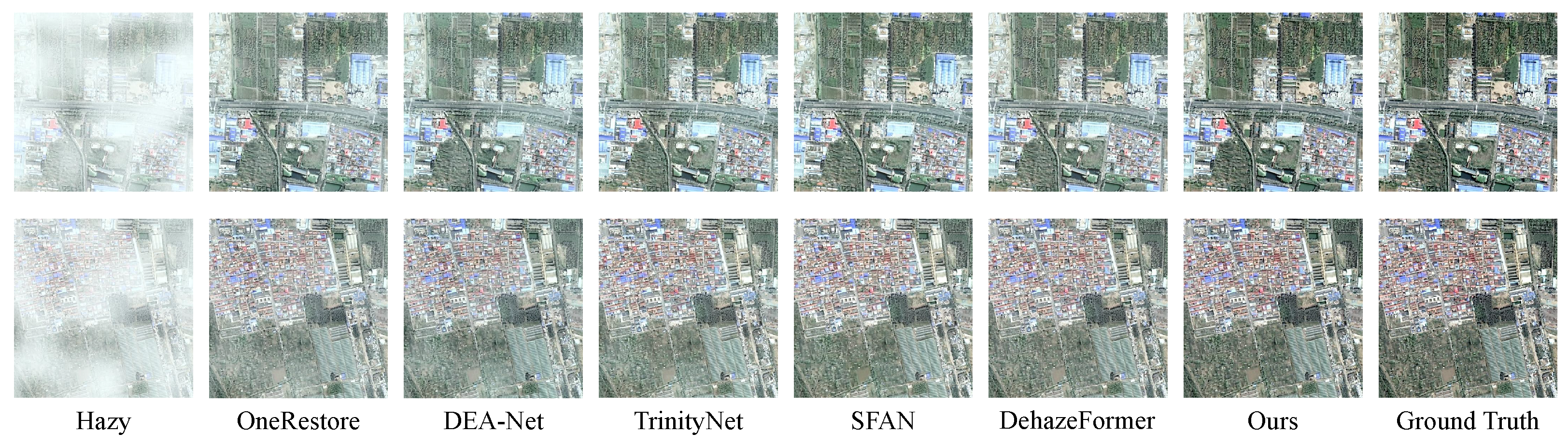
RICE1/2: On the harder RICE benchmarks, WaveDiff-R yielded consistent gains. On RICE1, it reached 36.709 dB PSNR and 0.986 SSIM, exceeding SFAN by + 0.06 dB PSNR and + 0.1 % SSIM, and surpassing DehazeFormer by + 0.25 dB PSNR. On RICE2, it obtained 34.187 dB PSNR— + 0.08 dB over SFAN and + 0.25 dB over DehazeFormer—while keeping 0.906 SSIM. Figure 5 illustrates the recovery of sharp edges and textures (terrain boundaries, rooftops, vegetation).
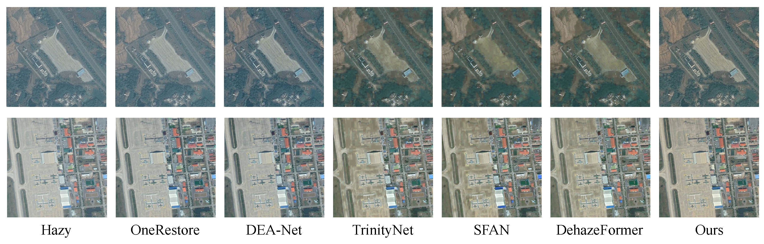
RSID: The RSID set couples haze with noise, illumination imbalance, and sensor distortions. WaveDiff-R achieved 26.203/0.954, improving over OneRestore (26.041/0.953) by + 0.162 dB and + 0.001 SSIM, and over SFAN (26.135/0.952) by + 0.068 dB and + 0.002 SSIM. We attribute the gains to the combination of VSSM-based global context modeling and sub-band residual enhancement, which together handle large-scale haze gradients and fine-scale texture loss (see Figure 6 for balanced contrast and spectral consistency).
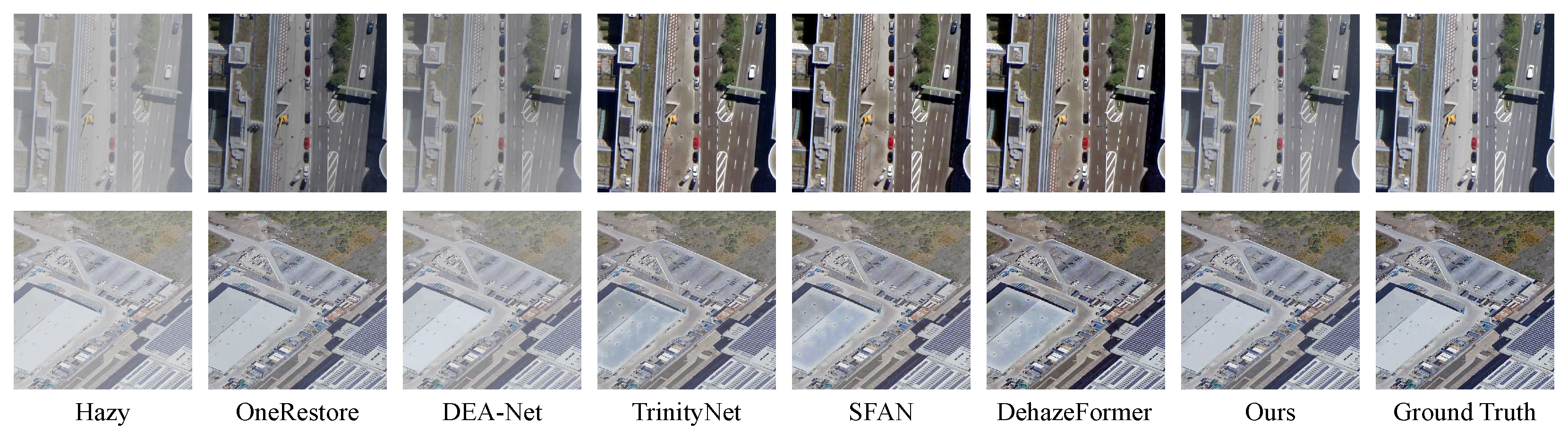
StateHaze1K (S-thin/S-moderate/S-thick). To probe the robustness across haze densities, we evaluated all methods on the three StateHaze1K subsets (Table 2); examples are in Figure 7.
S-thin: Most methods reached a high SSIM; subtle texture retention became the separator. WaveDiff-R attained the best PSNR (24.131 dB) and tied for the top SSIM (0.979) with OneRestore, outperforming it by + 0.101 dB PSNR ( + 0.42 % ). It also surpassed SFAN by + 0.443 dB PSNR ( + 1.87 % ) and + 0.016 SSIM ( + 1.66 % ), indicating the strong recovery of fine details under light haze.
S-moderate: When both the structure and color constancy matter, WaveDiff-R delivers 28.709 dB PSNR and 0.987 SSIM—gains of + 0.509 dB ( + 1.80 % ) and + 1.02 % SSIM over SFAN, and + 0.509 dB over OneRestore—showing the synergy between the WGDM’s global modeling and the RSEM’s sub-band enhancement.
S-thick: Under severe haze, low-frequency attenuation and contrast suppression cause many NSI models to degrade. WaveDiff-R reached 23.191 dB PSNR and 0.953 SSIM, surpassing OneRestore by + 0.071 dB and + 0.42 % SSIM, and SFAN by + 0.185 dB and + 1.17 % SSIM. Integrating physically grounded priors into the generative process helps restore contrast in heavily obscured areas without color bias.
Category-wise trends: NSI models (e.g., DehazeFormer, OneRestore) are competitive in light/moderate haze, but may over-smooth or lose texture in dense haze due to missing RSI priors. RSI models (e.g., SFAN, DCINet) maintain the spectral properties, but trail in subtle texture and global coherence. WaveDiff-R ranked first across all haze levels, with PSNR gains up to + 1.87 % over SFAN and + 2.26 % over OneRestore, evidencing cross-density adaptability.
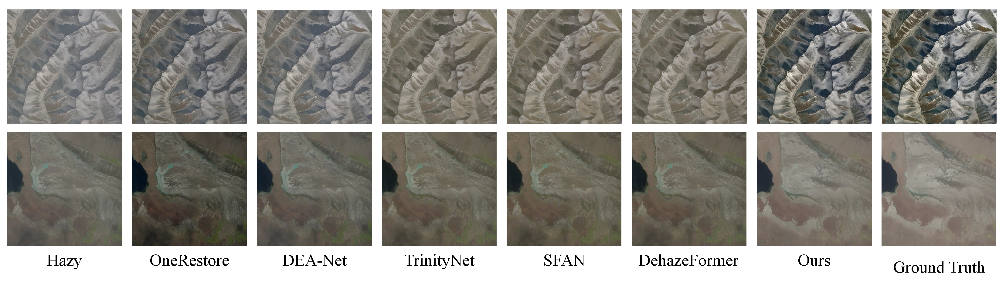
Real-world generalization (RRSD300): With no-reference metrics, WaveDiff-R attained the lowest scores (3.96 NIQE, 0.4329 FADE), indicating a better perceptual quality and haze removal (Table 3). Compared with DehazeFormer and SFAN, NIQE dropped by 6.9 % and 8.1 % , and FADE by 5.8 % and 6.5 % . Figure 8 shows uniform dehazing with balanced radiometry, avoiding residual haze and color distortion—properties desirable for downstream RS tasks.

6. Ablation Study

To quantify each component’s role, we ablated the WGDM, RSEM, and RSSB on S-moderate and LHID (Table 4); Δ denotes the drop relative to the full model.
Removing the WGDM lowered the PSNR by 0.520 dB (S-moderate) and 0.470 dB (LHID), with the SSIM being 0.012 on both. The WGDM thus helps preserve structure by steering the denoising with degradation-aware cues. Eliminating the RSEM caused the largest decline: PSNR 0.630 dB (S-moderate) and 0.550 dB (LHID), and SSIM 0.013 on both. Replacing the RSEM with a convolutional variant reduced the PSNR gaps to 0.414 dB and 0.362 dB, but the SSIM still dropped by 0.011 , indicating that the state space design captures broader dependencies than standard convolution. Substituting the RSSB with conventional convolution blocks yielded a PSNR 0.587 dB (S-moderate) and 0.502 dB (LHID), with an SSIM 0.012 . This supports the benefit of residual state space modeling for long-range interaction and global consistency. All three modules matter: the RSEM delivers the largest gains in fidelity (PSNR) and perceptual quality (SSIM), while the WGDM and RSSB complement it with degradation awareness and improved global coherence.

6.1. Ablation on K and Diffusion Sampling Step S

We examined how the RSEM segmentation count K and the diffusion sampling steps S affect the accuracy and runtime. As reported in Table 5, we evaluated K { 1 , 2 , 3 } and S { 5 , 10 , 20 , 30 } on S-moderate and LHID. For K, the best accuracy–speed balance was at K = 2 : it yielded up to + 0.16 dB PSNR on S-moderate and + 0.23 dB on LHID over K = 1 /3, while keeping the inference under 0.141 s per 256 × 256 image. A two-way split provides sufficient structural granularity without the overhead of finer partitions. For S, training with varied step counts makes the sampler robust: the PSNR changes by < 0.02 dB when S increases from 10 to 30. Unlike diffusion image generation [13,48], where a larger S often boosts the perceptual quality, here it mainly increases latency; GDP [49] and Palette [50] used up to S = 1000 , whereas our model attained state-of-the-art results with S = 10 . In practice, very large step counts are unnecessary for remote sensing dehazing; we adopted K = 2 and S = 10 by default, which gave the best accuracy on both datasets at a low cost.

6.2. Effect of Wavelet Bases

As shown in Table 6, WaveDiff-R remained stable under different wavelet bases, with only minor PSNR/SSIM fluctuations. Haar achieved the best overall performance and was adopted as the default setting due to its compact support, orthogonality, and efficient low-/high-frequency separation. Other bases, such as db2, sym2, and bior2.2, produce comparable results, indicating that the proposed frequency-selective diffusion framework is not overly sensitive to a specific wavelet choice. The slight advantage of Haar may come from its sharper spatial localization, which better preserves edge transitions in remote sensing scenes while keeping the low-frequency diffusion target compact.

7. Conclusions

In this paper, we introduced WaveDiff-R, a wavelet-guided diffusion framework for remote sensing image dehazing. The wavelet-guided diffusion module (WGDM) conditions the denoising trajectory with multiscale frequency cues, the residual state space block (RSSB) supplies efficient long-range dependency modeling, and the residual sub-band enhancement module (RSEM) targets wavelet sub-bands with adaptive granularity. Across six synthetic and real-world remote sensing datasets, WaveDiff-R consistently surpassed both natural-image (NSI) and remote sensing-specific (RSI) baselines, delivering state-of-the-art PSNR/SSIM values with fewer diffusion sampling steps at inference. Ablation studies confirm the complementary roles of the WGDM, RSEM, and RSSB, and demonstrate robustness to the sub-band segmentation number K and the sampling-step count S. Overall, WaveDiff-R offers a principled route to fusing frequency-domain priors with diffusion for scalable, radiometrically stable remote sensing restoration. In future work, we plan to extend WaveDiff-R to handle more complex atmospheric conditions such as mixed weather degradations, and to explore its application to other high-resolution remote sensing restoration tasks, including shadow removal and cloud removal.

Author Contributions

Methodology, M.Z.; software, M.Z.; validation, M.Z.; writing—original draft, M.Z.; writing—review and editing, M.Z.; supervision, S.Y. All authors have read and agreed to the published version of the manuscript.

Funding

The work was supported by Anhui Vocational and the Adult Education Association Planning Project (AZCJ2024212), Chuzhou Polytechnic Natural Science Research Project (ZKZ-2025-1), and by the Chuzhou Polytechnic Science and Technology InnovationPlatform Project (YJP-2023-02).

Data Availability Statement

The original contributions presented in this study are included in the article. Further inquiries can be directed to the corresponding author.

Conflicts of Interest

The authors declare no conflicts of interest.

References

  1. Narasimhan, S.G.; Nayar, S.K. Chromatic framework for vision in bad weather. In Proceedings IEEE Conference on Computer Vision and Pattern Recognition. CVPR 2000 (Cat. No. PR00662); IEEE: New York, NY, USA, 2000; Volume 1, pp. 598–605. [Google Scholar]
  2. Fang, Y.; Sun, L.; Zheng, Y.; Wu, Z. Deformable convolution-enhanced hierarchical transformer with spectral-spatial cluster attention for hyperspectral image classification. IEEE Trans. Image Process. 2025, 34, 701–716. [Google Scholar] [CrossRef]
  3. Fang, W.; Zhang, G.; Zheng, Y.; Chen, Y. Multi-task learning for uav aerial object detection in foggy weather condition. Remote Sens. 2023, 15, 4617. [Google Scholar] [CrossRef]
  4. Wang, C.; Fang, W.; Li, X.; Yang, J.; Luo, L. Msod: A large-scale multi-scene dataset and a novel diagonal-geometry loss for sar object detection. IEEE Trans. Geosci. Remote Sens. 2025, 63, 5220413. [Google Scholar] [CrossRef]
  5. He, K.; Sun, J.; Tang, X. Single image haze removal using dark channel prior. IEEE Trans. Pattern Anal. Mach. Intell. 2010, 33, 2341–2353. [Google Scholar] [CrossRef] [PubMed]
  6. Berman, D.; Treibitz, T.; Avidan, S. Single image dehazing using haze-lines. IEEE Trans. Pattern Anal. Mach. Intell. 2018, 42, 720–734. [Google Scholar] [CrossRef] [PubMed]
  7. Zhu, Q.; Mai, J.; Shao, L. A fast single image haze removal algorithm using color attenuation prior. IEEE Trans. Image Process. 2015, 24, 3522–3533. [Google Scholar] [CrossRef] [PubMed]
  8. Yu, H.; Zheng, N.; Zhou, M.; Huang, J.; Xiao, Z.; Zhao, F. Frequency and spatial dual guidance for image dehazing. In Proceedings of the European Conference on Computer Vision; Springer: Berlin/Heidelberg, Germany, 2022; pp. 181–198. [Google Scholar]
  9. Chen, Z.; He, Z.; Lu, Z.M. DEA-Net: Single image dehazing based on detail-enhanced convolution and content-guided attention. IEEE Trans. Image Process. 2024, 33, 1002–1015. [Google Scholar] [CrossRef] [PubMed]
  10. Guo, Y.; Gao, Y.; Lu, Y.; Zhu, H.; Liu, R.W.; He, S. Onerestore: A universal restoration framework for composite degradation. In Proceedings of the European Conference on Computer Vision; Springer: Berlin/Heidelberg, Germany, 2024; pp. 255–272. [Google Scholar]
  11. Chen, X.; Huang, Y. Memory-oriented unpaired learning for single remote sensing image dehazing. IEEE Geosci. Remote Sens. Lett. 2022, 19, 3511705. [Google Scholar] [CrossRef]
  12. Zheng, Y.; Su, J.; Zhang, S.; Tao, M.; Wang, L. Dehaze-AGGAN: Unpaired remote sensing image dehazing using enhanced attention-guide generative adversarial networks. IEEE Trans. Geosci. Remote Sens. 2022, 60, 5630413. [Google Scholar] [CrossRef]
  13. Ho, J.; Jain, A.; Abbeel, P. Denoising diffusion probabilistic models. Adv. Neural Inf. Process. Syst. 2020, 33, 6840–6851. [Google Scholar]
  14. Bansal, A.; Borgnia, E.; Chu, H.M.; Li, J.; Kazemi, H.; Huang, F.; Goldblum, M.; Geiping, J.; Goldstein, T. Cold diffusion: Inverting arbitrary image transforms without noise. Adv. Neural Inf. Process. Syst. 2023, 36, 41259–41282. [Google Scholar] [CrossRef]
  15. Lv, X.; Zhang, S.; Wang, C.; Zheng, Y.; Zhong, B.; Li, C.; Nie, L. Fourier priors-guided diffusion for zero-shot joint low-light enhancement and deblurring. In Proceedings of the IEEE/CVF Conference on Computer Vision and Pattern Recognition; IEEE: New York, NY, USA, 2024; pp. 25378–25388. [Google Scholar]
  16. Lugmayr, A.; Danelljan, M.; Romero, A.; Yu, F.; Timofte, R.; Van Gool, L. Repaint: Inpainting using denoising diffusion probabilistic models. In Proceedings of the IEEE/CVF Conference on Computer Vision and Pattern Recognition; IEEE: New York, NY, USA, 2022; pp. 11461–11471. [Google Scholar]
  17. Lan, Y.; Cui, Z.; Liu, C.; Peng, J.; Wang, N.; Luo, X.; Liu, D. Exploiting Diffusion Prior for Real-World Image Dehazing with Unpaired Training. arXiv 2025, arXiv:2503.15017. [Google Scholar]
  18. Mardani, M.; Song, J.; Kautz, J.; Vahdat, A. A variational perspective on solving inverse problems with diffusion models. arXiv 2023, arXiv:2305.04391. [Google Scholar]
  19. Fang, W.; Fan, J.; Wang, C.; Hu, X.; Weng, J.; Tai, Y.; Yang, J.; Li, J. When color-space decoupling meets diffusion for adverse-weather image restoration. arXiv 2025, arXiv:2509.17024. [Google Scholar]
  20. Song, Y.; He, Z.; Qian, H.; Du, X. Vision transformers for single image dehazing. IEEE Trans. Image Process. 2023, 32, 1927–1941. [Google Scholar] [CrossRef] [PubMed]
  21. Shen, H.; Zhao, Z.Q.; Zhang, Y.; Zhang, Z. Mutual information-driven triple interaction network for efficient image dehazing. In Proceedings of the 31st ACM International Conference on Multimedia; Association for Computing Machinery: New York, NY, USA, 2023; pp. 7–16. [Google Scholar]
  22. Lihe, Z.; He, J.; Yuan, Q.; Jin, X.; Xiao, Y.; Zhang, L. Phdnet: A novel physic-aware dehazing network for remote sensing images. Inf. Fusion 2024, 106, 102277. [Google Scholar] [CrossRef]
  23. Bie, Y.; Yang, S.; Huang, Y. Single remote sensing image dehazing using gaussian and physics-guided process. IEEE Geosci. Remote Sens. Lett. 2022, 19, 3512405. [Google Scholar] [CrossRef]
  24. Zhang, K.; Ma, S.; Zheng, R.; Zhang, L. UAV remote sensing image dehazing based on double-scale transmission optimization strategy. IEEE Geosci. Remote Sens. Lett. 2022, 19, 6516305. [Google Scholar] [CrossRef]
  25. Shen, H.; Ding, H.; Zhang, Y.; Cong, X.; Zhao, Z.Q.; Jiang, X. Spatial-frequency adaptive remote sensing image dehazing with mixture of experts. IEEE Trans. Geosci. Remote Sens. 2024, 62, 4211114. [Google Scholar] [CrossRef]
  26. Huang, Y.; Xiong, S. Remote sensing image dehazing using adaptive region-based diffusion models. IEEE Geosci. Remote Sens. Lett. 2023, 20, 8001805. [Google Scholar] [CrossRef]
  27. Li, S.; Zhou, Y.; Kung, S.Y. PSRNet: A Progressive Self-refine Network for Lightweight Optical Remote Sensing Image Dehazing. IEEE Trans. Geosci. Remote Sens. 2024, 62, 5648413. [Google Scholar] [CrossRef]
  28. Nichol, A.Q.; Dhariwal, P. Improved denoising diffusion probabilistic models. In Proceedings of the International Conference on Machine Learning; PMLR: Cambridge, MA, USA, 2021; pp. 8162–8171. Available online: https://arxiv.org/abs/2102.09672 (accessed on 3 July 2026).
  29. Luo, Z.; Gustafsson, F.K.; Zhao, Z.; Sjölund, J.; Schön, T.B. Image restoration with mean-reverting stochastic differential equations. arXiv 2023, arXiv:2301.11699. [Google Scholar]
  30. Song, D.; Yan, Q.; Wang, H.; Yang, J.; Luo, X. Wavelet-guided diffusion enhancement network with directional learning for single-pixel imaging. Pattern Recognit. 2025, 172, 112322. [Google Scholar]
  31. Li, X.; Wu, S.; Yuan, X.; Xie, S.; Agaian, S. Hierarchical wavelet-guided diffusion model for single image deblurring. Vis. Comput. 2025, 41, 3785–3800. [Google Scholar]
  32. Heil, C.E.; Walnut, D.F. Continuous and discrete wavelet transforms. SIAM Rev. 1989, 31, 628–666. [Google Scholar] [CrossRef]
  33. Stanković, R.S.; Falkowski, B.J. The Haar wavelet transform: Its status and achievements. Comput. Electr. Eng. 2003, 29, 25–44. [Google Scholar] [CrossRef]
  34. Guo, H.; Li, J.; Dai, T.; Ouyang, Z.; Ren, X.; Xia, S.T. Mambair: A simple baseline for image restoration with state-space model. In Proceedings of the European Conference on Computer Vision; Springer: Berlin/Heidelberg, Germany, 2024; pp. 222–241. [Google Scholar]
  35. Huang, B.; Zhi, L.; Yang, C.; Sun, F.; Song, Y. Single satellite optical imagery dehazing using SAR image prior based on conditional generative adversarial networks. In Proceedings of IEEE/CVF Winter Conference on Applications of Computer Vision; IEEE: New York, NY, USA, 2020; pp. 1806–1813. [Google Scholar]
  36. Chi, K.; Yuan, Y.; Wang, Q. Trinity-Net: Gradient-guided Swin transformer-based remote sensing image dehazing and beyond. IEEE Trans. Geosci. Remote Sens. 2023, 61, 4702914. [Google Scholar] [CrossRef]
  37. Zhang, L.; Wang, S. Dense haze removal based on dynamic collaborative inference learning for remote sensing images. IEEE Trans. Geosci. Remote Sens. 2022, 60, 5631016. [Google Scholar] [CrossRef]
  38. Lin, D.; Xu, G.; Wang, X.; Wang, Y.; Sun, X.; Fu, K. A remote sensing image dataset for cloud removal. arXiv 2019, arXiv:1901.00600. [Google Scholar]
  39. Li, K.; Wan, G.; Cheng, G.; Meng, L.; Han, J. Object detection in optical remote sensing images: A survey and a new benchmark. ISPRS J. Photogramm. Remote Sens. 2020, 159, 296–307. [Google Scholar] [CrossRef]
  40. Zheng, Z.; Ren, W.; Cao, X.; Hu, X.; Wang, T.; Song, F.; Jia, X. Ultra-high-definition image dehazing via multi-guided bilateral learning. In Proceedings of the 2021 IEEE/CVF Conference on Computer Vision and Pattern Recognition (CVPR); IEEE: New York, NY, USA, 2021; pp. 16180–16189. [Google Scholar]
  41. Wu, H.; Qu, Y.; Lin, S.; Zhou, J.; Qiao, R.; Zhang, Z.; Xie, Y.; Ma, L. Contrastive learning for compact single image dehazing. In Proceedings of the IEEE/CVF Conference on Computer Vision and Pattern Recognition; IEEE: New York, NY, USA, 2021; pp. 10551–10560. [Google Scholar]
  42. Guo, C.L.; Yan, Q.; Anwar, S.; Cong, R.; Ren, W.; Li, C. Image dehazing transformer with transmission-aware 3d position embedding. In Proceedings of the IEEE/CVF Conference on Computer Vision and Pattern Recognition; IEEE: New York, NY, USA, 2022; pp. 5812–5820. [Google Scholar]
  43. Li, J.; Hu, Q.; Ai, M. Haze and thin cloud removal via sphere model improved dark channel prior. IEEE Geosci. Remote Sens. Lett. 2018, 16, 472–476. [Google Scholar] [CrossRef]
  44. Han, J.; Zhang, S.; Fan, N.; Ye, Z. Local patchwise minimal and maximal values prior for single optical remote sensing image dehazing. Inf. Sci. 2022, 606, 173–193. [Google Scholar] [CrossRef]
  45. Li, Y.; Chen, X. A coarse-to-fine two-stage attentive network for haze removal of remote sensing images. IEEE Geosci. Remote Sens. Lett. 2020, 18, 1751–1755. [Google Scholar]
  46. Wen, Y.; Gao, T.; Zhang, J.; Li, Z.; Chen, T. Encoder-free multiaxis physics-aware fusion network for remote sensing image dehazing. IEEE Trans. Geosci. Remote Sens. 2023, 61, 4705915. [Google Scholar] [CrossRef]
  47. Sun, H.; Luo, Z.; Ren, D.; Hu, W.; Du, B.; Yang, W.; Wan, J.; Zhang, L. Partial siamese with multiscale bi-codec networks for remote sensing image haze removal. IEEE Trans. Geosci. Remote Sens. 2023, 61, 4106516. [Google Scholar] [CrossRef]
  48. Song, Y.; Sohl-Dickstein, J.; Kingma, D.P.; Kumar, A.; Ermon, S.; Poole, B. Score-based generative modeling through stochastic differential equations. arXiv 2020, arXiv:2011.13456. [Google Scholar]
  49. Fei, B.; Lyu, Z.; Pan, L.; Zhang, J.; Yang, W.; Luo, T.; Zhang, B.; Dai, B. Generative diffusion prior for unified image restoration and enhancement. In Proceedings of the IEEE/CVF Conference on Computer Vision and Pattern Recognition; IEEE: New York, NY, USA, 2023; pp. 9935–9946. [Google Scholar]
  50. Saharia, C.; Chan, W.; Chang, H.; Lee, C.; Ho, J.; Salimans, T.; Fleet, D.; Norouzi, M. Palette: Image-to-image diffusion models. In Proceedings of the ACM SIGGRAPH 2022 Conference Proceedings; Association for Computing Machinery: New York, NY, USA, 2022; pp. 1–10. [Google Scholar]
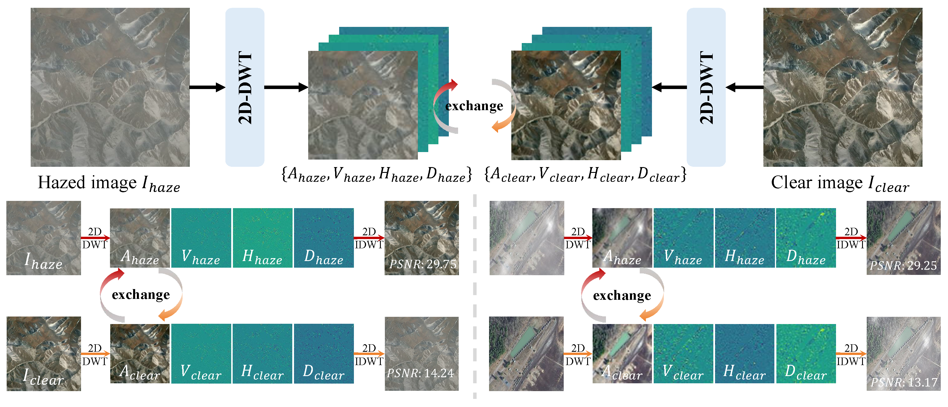
Figure 1. Frequency-switching experiment in remote sensing haze images. Haze mainly depresses the low-frequency band A, shifting the luminance and color, while high-frequency sub-bands retain the structure, but lose sharpness. Replacing A hazy with A clear restores the global contrast and color; replacing only the high-frequency bands sharpens the textures, yet leaves the global haze.
Atmosphere 17 00684 g001
Figure 2. Overall architecture of the proposed WaveDiff-R.
Atmosphere 17 00684 g002
Figure 3. Structure of the residual state space block (RSSB). High-frequency sub-bands are processed via a global VSSM branch for long-range dependency modeling and a local depthwise convolution branch for texture refinement, followed by feature fusion and residual connection.
Atmosphere 17 00684 g003
Figure 4. Qualitative comparison of dehazing methods on DHID and LHID datasets.
Atmosphere 17 00684 g004
Figure 5. Visual comparison with state-of-the-art methods on RICE1 and RICE2 datasets.
Atmosphere 17 00684 g005
Figure 6. Dehazing performance on the RSID dataset. In contrast to existing methods—such as DehazeFormer, DEA-Net, and SFAN—which often suffer from over-smoothing, color shifts, or residual haze, our approach effectively restores sharp structural details and natural color fidelity, particularly in sky, vegetation, and building areas.
Atmosphere 17 00684 g006
Figure 7. Comparison of dehazing methods using the StateHaze1K dataset, composed of large-scale, geographically diverse remote sensing scenes with synthetic haze.
Atmosphere 17 00684 g007
Figure 8. Visual assessment of dehazing methods on the RRSD300 dataset, which features real-world hazy satellite and aerial imagery.
Atmosphere 17 00684 g008
Table 1. Quantitative evaluation of dehazing methods on five benchmark datasets. Top-performing and runner-up results are highlighted in red and blue.
TypeMethodsVenueDHIDLHIDRICE1RICE2RSID
PSNRSSIMPSNRSSIMPSNRSSIMPSNRSSIMPSNRSSIM
NSI dehazing methods4KDehazing [40]CVPR’2127.4660.93329.2000.95327.2220.94127.5290.91523.3850.915
AECRNet [41]CVPR’2128.6140.93832.3500.96424.0550.92126.2570.77021.8390.889
DeHamer [42]CVPR’2228.0400.93528.2330.94130.9560.94729.7520.85122.3690.848
FSDGN [8]ECCV’2228.7930.93633.5090.96733.4200.98231.0170.85825.3980.946
MITNet [21]ACM’2327.6680.93829.5020.95233.4500.97931.0860.87324.2430.935
DehazeFormer [20]TIP’2327.5250.93131.6060.96236.4640.98233.8350.88625.6220.946
PhDnet-S [22]INFFUS’2426.8980.93133.0910.96736.2460.98233.9330.89525.8940.950
DEA-Net [9]TIP’2427.3180.93333.4510.96735.2440.98334.0100.89125.9180.951
OneRestore [10]ECCV’2428.7740.93933.9510.96636.4130.98034.1030.88126.0410.953
RSI dehazing methodsSDCP [43]GRSL’1811.3920.18212.2410.16014.0860.37614.8960.37617.20617.206
MinVP [44]INS’1811.3700.17814.3810.19618.8890.91916.5050.54417.8710.803
FCTFNet [45]GRSL’2024.9290.90730.0470.96431.4070.97531.5260.87222.9760.919
DCINet [37]TGRS’2228.8650.93828.3200.94129.8120.95825.6280.79324.4990.928
EMPFNet [46]TGRS’2325.5020.92030.2320.95831.5520.96928.9990.84621.7080.912
PSMBNet [47]TGRS’2328.3330.93531.8700.96527.9790.93928.1340.84723.2620.925
TrinityNet [36]TGRS’2316.1890.91327.2190.93829.6590.95928.8360.85624.1960.927
SFAN [25]TGRS’2429.1730.94234.0290.97036.6530.98534.0950.98726.1350.952
WaveDiff-R (Ours)-29.3130.94734.1740.97336.7090.98634.1870.90626.2030.954
Table 2. Quantitative comparision of dehazing methods on StateHaze1K dataset. Top-performing and runner-up results are highlighted in red and blue.
TypeMethodsS-ThinS-ModerateS-Thick
PSNRSSIMPSNRSSIMPSNRSSIM
NSI dehazing methodsAECRNet [41]23.9570.96726.0910.95821.4570.924
DeHamer [42]22.7680.93326.3710.94322.3690.899
FSDGN [8]21.7300.94626.3710.94322.3510.937
MITNet [21]22.0540.95023.6370.93620.1900.918
DehazeFormer [20]23.0220.96023.0910.97322.6710.939
DEA-Net [9]23.5120.96126.9710.97322.9830.938
OneRestore [10]24.0300.97928.2000.97723.1200.949
RSI dehazing methodsSDCP [43]14.1860.82516.0680.78616.3850.842
MinVP [44]20.9670.93721.0460.91316.5880.863
FCTFNet [45]23.3270.95826.4390.96820.7520.917
DCINet [37]20.1870.94727.4310.96421.4500.926
EMPFNet [46]23.4340.95625.7930.96319.4870.912
PSMBNet [47]22.9460.94927.9210.96021.2730.919
TrinityNet [36]21.3040.94626.4730.91520.7560.915
SFAN [25]23.6880.96328.1910.97723.0060.942
WaveDiff-R (Ours)24.1310.97928.7090.98723.1910.953
Table 3. Quantitative evaluation of dehazing approaches on RRSD300. For NIQE and FADE, smaller values signify higher perceptual quality and fewer haze artifacts.
MethodsNIQE ↓FADE ↓
Hazy5.811.4351
4KDehazing [40]5.600.8843
DCINet [37]5.170.5487
DeHamer [42]5.210.7268
DehazeFormer [20]5.030.5591
DEA-Net [9]5.340.5570
SFAN [25]4.910.5239
WaveDiff-R (Ours)3.370.4107
Table 4. Ablation results for WGDM, RSEM, and RSSB on S-moderate and LHID datasets. Δ denotes performance drop relative to the full model.
VariantS-ModerateLHID
PSNR/ Δ SSIM/ Δ PSNR/ Δ SSIM/ Δ
Full model28.709/-0.987/-34.174/-0.973/-
w/o WGDM28.189/↓0.5200.975/↓0.01233.704/↓0.4700.961/↓0.012
w/o RSEM28.079/↓0.6300.974/↓0.01333.624/↓0.5500.960/↓0.013
Conv-based RSEM28.295/↓0.4140.976/↓0.01133.812/↓0.3620.962/↓0.011
w/o RSSB (Conv Blocks)28.122/↓0.5870.975/↓0.01233.672/↓0.5020.961/↓0.012
Table 5. Ablation study of K (RSEM segments) and diffusion sampling step S on S-moderate and LHID datasets. Time is measured per 512 × 512 image.
Wavelet Scale KSampling Step SS-ModerateLHIDTime (s)
PSNRSSIMPSNRSSIM
K = 1528.4120.98333.8920.9690.186
1028.5660.98433.9810.9700.366
2028.6010.98434.0120.9700.737
3028.5890.98434.0010.9701.110
K = 2528.5910.98534.0910.9720.073
1028.7090.98734.1740.9730.141
2028.6880.98634.1620.9730.269
3028.6920.98634.1680.9730.443
K = 3528.3220.98333.8420.9690.049
1028.4710.98433.9310.9700.109
2028.4980.98433.9450.9700.204
3028.5010.98433.9520.9700.361
Table 6. Performance comparison of different wavelet bases on S-moderate and LHID datasets. ( Δ ) denotes the performance drop relative to the default Haar wavelet.
Wavelet BasisS-ModerateLHID
PSNR/( Δ )SSIM/( Δ ) PSNR/( Δ ) SSIM/( Δ )
Haar (Default)28.709/–0.987/–34.174/–0.973/–
Daubechies-2 (db2)28.642/(↓ 0.067)0.986/(↓ 0.001)34.106/(↓ 0.068)0.972/(↓ 0.001)
Daubechies-4 (db4)28.611/(↓ 0.098)0.985/(↓ 0.002)34.083/(↓ 0.091)0.971/(↓ 0.002)
Symlet-2 (sym2)28.657/(↓ 0.052)0.986/(↓ 0.001)34.121/(↓ 0.053)0.972/(↓ 0.001)
Coiflet-1 (coif1)28.596/(↓ 0.113)0.985/(↓ 0.002)34.061/(↓ 0.113)0.971/(↓ 0.002)
Biorthogonal-2.2 (bior2.2)28.624/(↓ 0.085)0.986/(↓ 0.001)34.094/(↓ 0.080)0.972/(↓ 0.001)
Disclaimer/Publisher’s Note: The statements, opinions and data contained in all publications are solely those of the individual author(s) and contributor(s) and not of MDPI and/or the editor(s). MDPI and/or the editor(s) disclaim responsibility for any injury to people or property resulting from any ideas, methods, instructions or products referred to in the content.