Article

Six-Month Lasting Observations of Submicron Non-Refractory Aerosol Particles by Time-of-Flight Aerosol Chemical Speciation Monitor (ToF-ACSM) at CIAO (Potenza, Italy)


1
Institute of Methodologies for Environmental Analysis, National Research Council of Italy (CNR-IMAA), Contrada S. Loja, Tito Scalo, I-85050 Potenza, Italy
2
Department of Engineering, University of Basilicata (Unibas DiING), Via dell’Ateneo Lucano 10, I-85100 Potenza, Italy
*
Author to whom correspondence should be addressed.
Atmosphere 2026, 17(7), 677; https://doi.org/10.3390/atmos17070677
Submission received: 3 June 2026 / Revised: 4 July 2026 / Accepted: 6 July 2026 / Published: 8 July 2026
(This article belongs to the Section Aerosols)

Abstract

As part of the ACTRIS research infrastructure, a six-month study (May–October 2024) was conducted at the CNR-IMAA Atmospheric Observatory (CIAO, Southern Italy) to characterize non-refractory submicron aerosol (NR-PM1). Measurements were conducted in real time using a time-of-flight aerosol chemical speciation monitor (ToF-ACSM) and highlighted the predominant presence of organic aerosol (OA), with values reaching 49.5 µg m−3. During the study period, nitrate and ammonium concentrations remained below 2 µg m−3 on average, while sulfate concentrations showed normal variation during the analysis period (maximum value of 11.70 µg m−3). The daily variability of concentrations was influenced by both boundary layer dynamics and local emission variations. The calculated charge and mass balances allowed us to study the good neutralization of PM1 in the atmosphere. The composition of the organic aerosol was dominated by oxygenated species, with a small contribution from biomass combustion. Ultimately, these results provide an excellent starting point for understanding the aerosol chemical composition and seasonal variability at the site, ahead of future analyses and comparisons within the ACTRIS of which the observatory is part.

1. Introduction

Atmospheric aerosols play a central role due to their ability to scatter and absorb radiation and act as cloud condensation nuclei, thus influencing both the Earth’s radiation budget and the hydrogeological cycle [1,2,3,4]. While the chemical and physical variability of aerosols significantly influences both meteorological and climate processes [5,6,7,8,9,10,11,12,13], the effects on human health are becoming increasingly evident, including respiratory and cardiovascular diseases [14,15,16,17]. In fact, according to the World Health Organization (WHO) recommendations on global air quality [18], more than 80% of the world’s population suffers from health problems due to air pollution and more than 8 million people die every year because of it [19]. For these reasons, further investigations of atmospheric aerosols are increasingly needed to improve our understanding of their sources, properties, and environmental impacts.
The most common observations in atmospheric studies are based on direct physical measurements and remote sensing from ground stations and satellites. As regards ground-based atmospheric information, most research has focused on the study of the chemical and physical characteristics of PM10 and PM2.5 particulate matter; only in recent years has particular attention been paid to the submicron fraction PM1, which can cause much more serious damage to human health than other fractions due to its easier access to the respiratory system [20,21]. PM1 consists of a complex mixture of organic and inorganic substances in solid and liquid phases that can remain suspended in the atmosphere for variable periods depending on their physicochemical properties. In general, it is worth emphasizing that smaller particles tend to remain suspended in the air for longer, to be transported over greater distances and undergo atmospheric aging and secondary chemical transformations more readily than larger particles.
Organic aerosols (OA) represent a major component of atmospheric particulate matter and play an important role in air quality, atmospheric chemistry and radiative forcing [22,23]. OA consist of a highly complex mixture of thousands of carbon-containing compounds, including hydrocarbons, oxygenated organic compounds, alcohols, aldehydes, organic acids, and other oxidation products [24]. OA sources can be classified as primary or secondary, with the latter mainly formed through reactions of precursors such as volatile organic compounds (VOCs) [25]. The relative contribution of VOCs sources varies significantly depending on spatial and temporal scales. While biogenic emissions dominate at the global scale, in urban and industrial environments anthropogenic sources, including industrial activities and solvent use, can account for a substantial share of total VOC emissions [26]. Given the complexity and variability of OA sources and formation pathways, detailed characterization of aerosol chemical composition is essential for understanding particle sources and atmospheric processing. Field measurements of aerosol chemical composition mainly use technologies based on particulate matter collection on in-line filters. Although these traditional methods are widely used and make important contributions to chemical composition assessment, their obvious limitations, including low temporal resolution (hours to days) and/or loss of volatile compounds due to evaporation or filter shear, limit their capabilities. In contrast, in-line mass spectrometry methods have higher temporal resolutions (ranging from seconds to hours) and have proven effective not only in measuring aerosol mass concentration but also chemical composition [27,28,29,30,31]. In recent years, the Time-of-Flight Aerosol Chemical Speciation Monitor (Tof-ACMS, Aerodyne Research Inc., Billerica, MA, USA) has been employed in numerous studies and has provided valuable chemical and microphysical information on submicron non-refractory aerosol particles (NR-PM1), due to the advantages of real-time, high-precision quantitative measurements [32,33].
Thanks to these characteristics, this type of instrumentation is used within the Aerosol, Clouds and Trace Gases Research Infrastructure (ACTRIS), the European Research Infrastructure (RI) whose objective is to integrate existing networks for the characterization of short-lived atmospheric constituents (SLAC) and clouds by coupling remote sensing and in situ observations (including ToF-ACSM observations). In this context, ACTRIS also provides a unique portfolio of services to be used by a large community of scientists [34,35]. As part of ACTRIS and given the complexity of studying aerosol particles, since 2018 the CNR-IMAA Atmospheric Observatory (CIAO) has received a significant upgrade of its capabilities with the acquisition of advanced instrumentation for the observation of the optical and chemical–physical properties of aerosols, including at ground level. This has allowed the CIAO to further strengthen its role in ACTRIS as a National Facility (NF). The combination of different techniques and observation platforms can be crucial for a better understanding of the characteristics of atmospheric aerosol particles, as well as their role in the wide variety of processes in which they are involved [36]. In fact, integrated approaches allow the acquisition of detailed information on the physical and chemical nature of particles and ground-level measurements provide important insights into how aerosol particles affect ecosystems and humans. This work presents the first results obtained from six months of NR-PM1 observations by ToF-ACSM at CIAO from May to October 2024. This represents the first study of the NR-PM1 fraction in this area. The statistically processed results presented demonstrate not only the reliability of the technique used, but above all its ability to identify the organic and inorganic components of the analyzed particles in real time. These aspects will also be crucial for understanding the sources of particle emissions, which could lead to a better understanding of local anthropogenic impacts and transport events.

2. Materials and Methods

2.1. CIAO Site Description

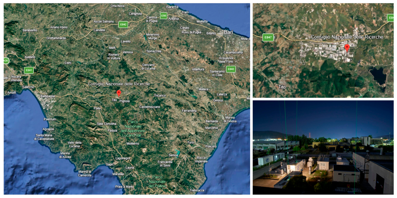
The CIAO is situated in Southern Italy, within the Southern Apennines (Tito Scalo–Basilicata region, 40.60° N, 15.72° E, 760 m a.s.l.), approximately 10 km northwest of Potenza, the regional capital (Figure 1). The station is in a flat area encircled by low-elevation mountains and rural zones rich in woodland, and it is less than 150 km from the Mediterranean coastline.
The surrounding territory includes several industrial facilities involved in the production of construction materials, steel structures, pharmaceutical goods, and electronic and mechanical components. The area is also characterized by a moderately busy road network, and the agricultural activities and livestock grazing are common near the measurement site.
Because of its location within the Mediterranean basin, the region is frequently influenced by intrusions of desert dust [37,38,39,40,41]. Episodes of volcanic ash transport have also been documented [42,43,44,45], together with aerosol particles originating from forest fires occurring both in nearby areas [46] and at long distances [47].
The local climate is typically mountainous and strongly modulated by Mediterranean atmospheric circulation, with hot, dry summers and cold winter conditions.

2.2. ToF-ACSM

Among the advanced ACTRIS-compliant instrumentation available at CIAO, a key role is played by the ToF-ACSM since it provides continuous near-real-time chemical characterization of non-refractory submicron particulate matter with high temporal resolution. This capability is necessary to improve our understanding of the mechanisms of formation and transformation of aerosol particles in the atmosphere and to identify the different sources and their contribution, even on short time scales.
The ToF-ACSM allows the determination of both the organic fraction of aerosols OA and inorganic components such as ammonium ion (NH4+), nitrate ion (NO3), sulfate ion (SO42−), and chloride ion (Cl). The operating principle of the ACSM [48] is based on the same principle previously used by Aerodyne for the aerosol mass spectrometer (AMS) [49,50]. Briefly, aerosols are sampled through an aerodynamic lens, where they are focused into a narrow beam and accelerated to a velocity inversely related to their aerodynamic size. The instrument has a PM1 lens, which provides the size cut. A PM2.5 cyclone upstream of the ACSM operating at 3 L min−1 is used to remove large particles, as they can cause inlet clogging [51]. The particles are transmitted into a high-vacuum detection chamber (∼10−5 Torr), where the NR-PM1 components impact a resistively heated surface (600 °C) and flash vaporize. The resulting gas molecules are ionized by electron impact (EI, ∼70 eV) and analyzed by time-of-flight mass spectrometry. Finally, the electrical signal is converted into a digital signal by the detector. A Nafion dryer installed upstream of the instrument eliminates the complicating inlet effects due to particle-composition-dependent water uptake [52].
Several calibrations must be performed regularly to ensure the accuracy of the instrument, according to the recommendations in the literature [53]. The instrument has a mass resolution (m/Δm) of 600 and detection limits < 1 ng m−3.

2.3. 7-Wavelength Aethalometer

In addition to the ToF-ACSM, information on black carbon (BC) was collected using an aethalometer. This instrument quantifies BC resulting from the incomplete combustion of organic material and can provide an estimate of the contribution of biomass combustion (BB) to the total BC. This allows the BC to be deconvoluted into the contribution of biomass combustion (BCbb) and the contribution of fossil fuels (BCff) and, therefore, the source contribution can be calculated. The model is based on the difference in absorption coefficients at different wavelengths; the exponents describing this difference are called Ångström absorption exponents (AE). The exponents used in this work were 1.0 for fossil fuels and 2.0 for biomass combustion, according to the AE approach developed by Sandradewi et al. [54]. In this study, an ACTRIS-compliant aethalometer (MAGEE Scientific, model AE33-Dual Spot, Ljubljana, Slovenia) operating at seven different wavelengths ranging from 370 to 950 nm [55] was used for real-time determination of BC concentrations. In this study, we considered the signal at 880 nm, which represents the defining standard used for reporting black carbon concentration [56]. The instrument is equipped with a PM10 cut-off inlet and operates at 5 L min−1. To maintain relative humidity (RH) below 40% (as per ACTRIS recommendations), the aethalometer is equipped with a sample flow dryer (Magee Scientific) that uses a semi-permeable Nafion membrane. It should be noted that due to the different types of inlets used compared to the ToF-ACSM, this study does not make a direct comparison of the mass fractions between BC and NR-PM1 species. The interpretation of BC data is therefore limited to its temporal variability and does not assume particle size equivalence with the submicron fraction. Further analyses and processing, aimed at integrating and comparing this type of information, will be the subject of future chemical-physical characterization studies of particulate matter, conducted synergistically using the various types of instrumentation available at the observatory.

2.4. Meteorological Data

Meteorological data such as temperature (T), relative humidity (RH), atmospheric pressure (AP), precipitation amount (PA), wind direction (WD) and wind speed (WS) are continuously acquired by Vaisala AWS 310 meteorological stations at CIAO (Helsinki, Finland). According to ToF-ACSM observations, the meteorological data used in this study covers the period from May to October 2024.

3. Results

3.1. Characterization of Non-Refractory PM1 and Black Carbon in PM10

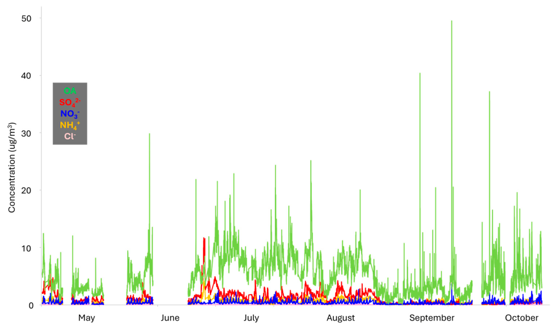
A total of ≈19,000 ACSM data points (with a temporal resolution of 10 min) were collected from May to October 2024, covering 74% of the period. Missing days in the time series corresponds to instrument maintenance operations or failure. Figure 2 reports the temporal pattern of the concentrations of the NR-PM1 species measured by ToF-ACSM in the period under study, while Table 1 summarizes the corresponding statistical parameters. As Figure 2 shows, OA is the main NR-PM1 component over the entire period. Until 7 September, sulphate is the main inorganic component, followed by ammonium and nitrate. After that date, the concentrations of inorganic species do not show significant differences. The organic component is characterized by an average concentration value of 5.02 µg/m3. Short-term pollution events lasting a few hours can also be observed, with peaks exceeding 20 µg/m3 and reaching a maximum value of 49.50 µg/m3. These episodes are likely associated with local emission events that are limited in time and space and potentially intensified under conditions of atmospheric stagnation and low boundary layer height, which limit the dispersion of the released species into the atmosphere. Observing the SO42− (sulphate) component, we note a decrease from May to October with an average concentration value of 1.16 µg/m3. This behavior may be related to natural variability in atmospheric oxidation processes and precursor availability, as well as changes in the contribution of long-range transport. Also in this case, we note some pollution events with peaks that reach the maximum value of 11.70 µg/m3 in July. As for the nitrogen component, NO3 and NH4+, unless there were pollution events, the values always settled below 2 µg/m3 and no significant fluctuations over time were noted. Finally, the concentration of Cl is not reported since it very often settles below the limit of detection (LoD—0.01 µg/m3).
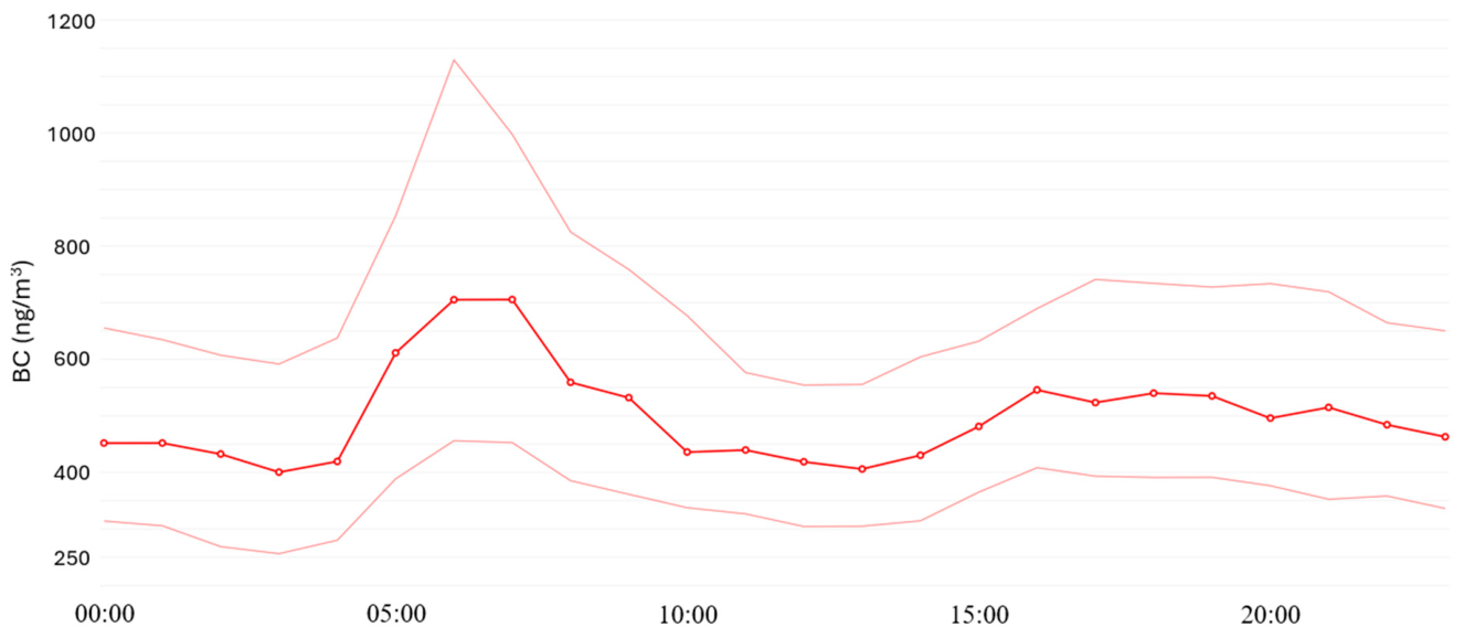
Figure 3 shows the daily BC concentration trend, calculated from the hourly mean BC concentration measured at the CIAO from May to August 2024. During September and October 2024, the instrument was located at the Leibniz Institute for Tropospheric Research in Leipzig, Germany, for calibration tests; therefore, BC data are not available. The absence of BC data for the last two months of the campaign represents a limitation of the dataset. Therefore, the analysis of BC temporal variability and its interpretation are restricted to the May–August period. While this subset captures a substantial portion of the campaign and provides a first characterization of BC variability at the site, potential variability occurring during the missing period cannot be evaluated and should be addressed in future investigations, where a more complete temporal coverage will allow for a more comprehensive assessment.
Black carbon (BC) concentrations show moderate diurnal variability, with peaks in the morning (06:00–09:00 UTC) and evening (17:00–22:00 UTC); this trend would suggest a partial connection with traffic emissions and atmospheric boundary layer dynamics. Indeed, during the central hours of the day, vertical mixing favors pollutant dilution, resulting in minimum levels in the early afternoon.
Despite this trend, typical of anthropogenic vehicular sources, the generally low daily mean concentrations (0.2–1.5 µg/m3) suggest that traffic is not the predominant source at the study site [57]. It is therefore plausible that other sources of black carbon also contribute, in a context where the direct influence of traffic is less pronounced.

3.2. Meteorological Parameters

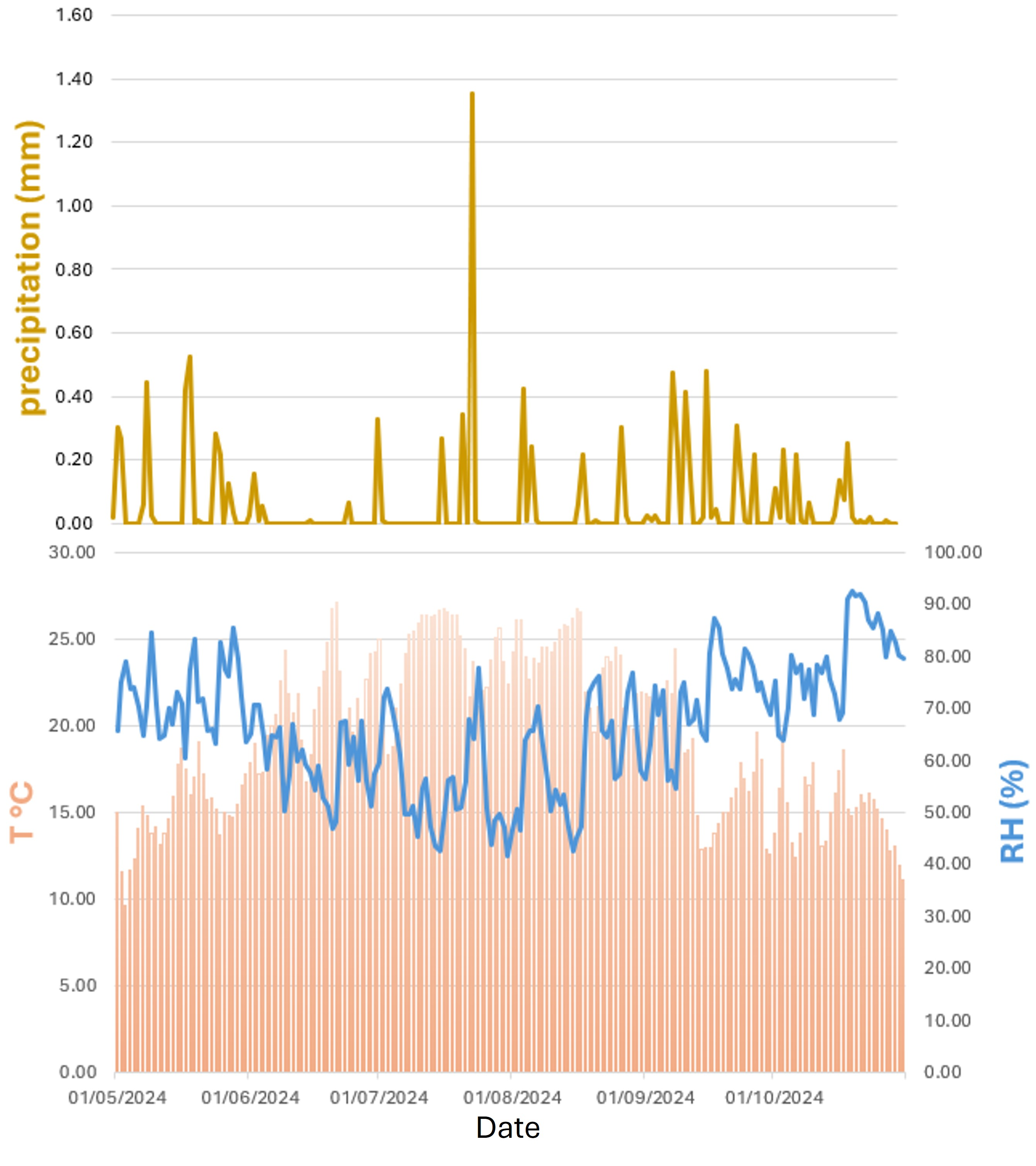
Figure 4 illustrates the temporal trends of T, RH, and PA recorded at the CIAO station over the study period. During this period, the weather was characterized by variable RH values, with hourly averages ranging from 41.5% to 92.4%. RH values above 85% were observed only under specific conditions and were often accompanied by precipitation.
T values remained below 30 °C, with hourly averages ranging from 9.0 °C to 27.0 °C. Its gradual increase from May to August and its decrease starting in September reflects the temporal evolution of meteorological conditions during the study period. Similarly, precipitation showed variability throughout the period, although total rainfall was relatively limited, amounting to 10.4 mm. These meteorological conditions are expected to play an important role in influencing aerosol concentrations and composition. T variations may affect chemical reaction rates and gas-to-particle partitioning processes, while RH can promote aqueous-phase reactions and influence particle hygroscopic growth. Understanding these meteorological conditions is important for interpreting aerosol variability and provides useful information for future long-term studies on atmospheric and climate-related processes.
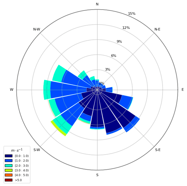
Finally, Figure 5 illustrates the wind rose calculated for the entire period. Wind intensity during the study period was generally low to moderate. Winds from the SW sector, which represented the prevailing direction, typically had speeds between 3 and 4 m s−1, while winds from the S and W sectors were weaker, with speeds of 1–2 m s−1 and 2–3 m s−1, respectively. These conditions may affect pollutant dispersion and transport, thereby influencing the observed temporal variability of aerosol species.

3.3. Diurnal, Weekly and Monthly Profiles of NR-PM1 Concentrations

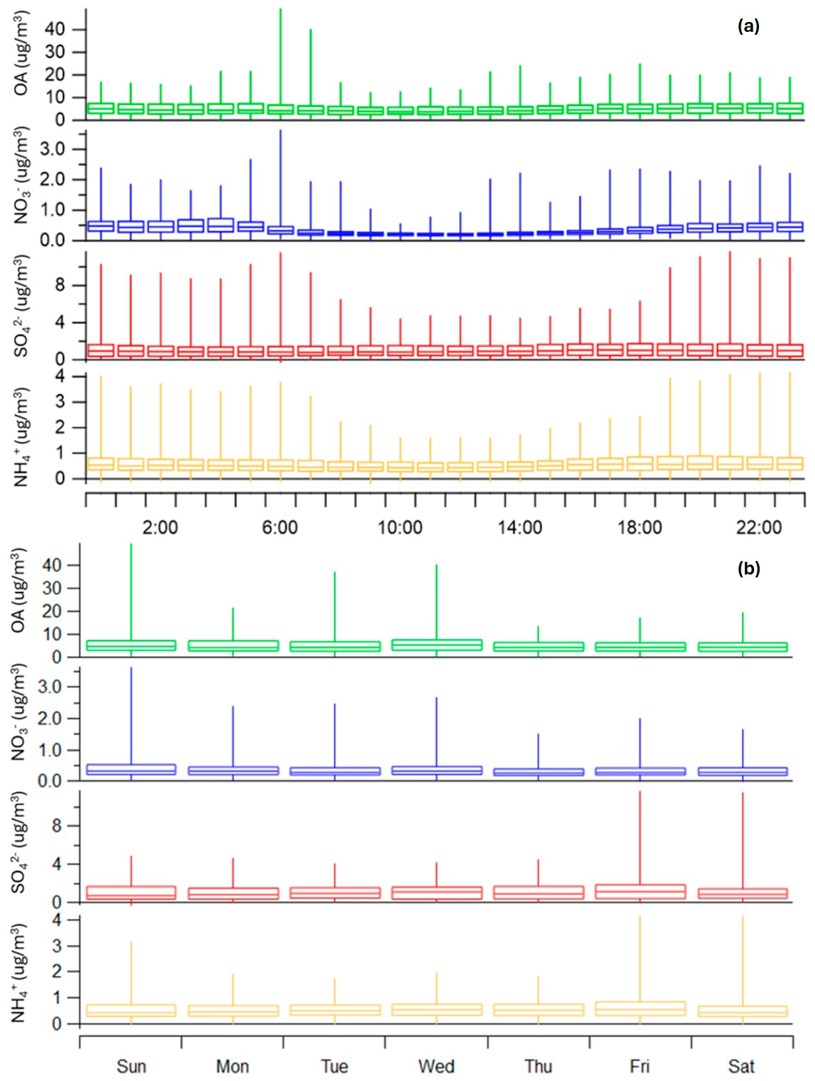
Figure 6a, b illustrate respectively the average diurnal and weekly behavior of OA, SO42−, NO3, and NH4+ during the entire analysis period. As previously mentioned, Cl is not reported as its values are mainly below the limit of detection.
All aerosol species (OA, NH4+, NO3 and SO42−) exhibit a coherent diurnal pattern, with minimum concentrations in the late morning and an increase during the afternoon and evening. This diurnal pattern may be likely influenced by boundary layer dynamics and temperature-driven changes in atmospheric mixing throughout the day.
Typical concentrations, represented by the median values, clearly show this behavior. OA reaches its lowest median values between 10:00 and 12:00 UTC (≈3.70 μg m−3), followed by a progressive rise toward the evening, around 20:00–22:00 UTC with median values in the range 5.00–5.50 μg m−3. NH4+ and NO3 show a similar evolution with NH4+ median that reaches its lowest value between 09:00 and 12:00 UTC (≈0.42 μg m−3) and increases toward the evening, reaching ≈0.56 μg m−3 after 19:00 UTC. NO3, characterized by its semi-volatile behavior, has low median values, equal to approximately ≈0.20 μg m−3, during the late morning and reaches higher values in the evening, up to ≈0.39 μg m−3 between 20:00 and 23:00 UTC. A similar but more moderate trend is observed for SO42− that reaches its lowest median values between 10:00 and 12:00 UTC (≈0.82 μg m−3) and increases it in the evening reaching ≈1.01 μg m−3. The interquartile range (Q1–Q3) reflects this pattern, with Q3 increasing from morning to evening for all species. For example, OA increases from ≈6.01 μg m−3 at 10:00 UTC to ≈7.55 μg m−3 in the late evening, while SO42− increases from ≈1.47 μg m−3 in the early morning to ≈1.77 μg m−3 in the evening.
Although the variation in these values describes a typical diurnal pattern, the maximum concentrations recorded across the entire dataset reveal the presence of pronounced peaks, associated with episodes. The highest concentration values for all species were frequently observed in the early morning hours, particularly between 06:00 and 08:00 UTC. These conditions may be consistent with stable nocturnal stratification, low wind speed, and reduced boundary layer height, which limits vertical mixing and favor pollutant accumulation near the surface. For example, OA reached a maximum value of 49.50 μg m−3 at 07:00 UTC, and similarly high peaks were recorded for NH4+ (up to 3.79 μg m−3 at 07:00 UTC), NO3 (up to 3.65 μg m−3 at 07:00 UTC), and SO42− (with maxima around 10–12 μg m−3 in the early morning hours). These maximum values do not coincide exclusively with peak traffic hours, which suggests that they are related to the accumulation of particulate matter in stable conditions of the nighttime boundary layer, local orography, and temperature inversions that inhibit vertical mixing. Therefore, these values in the early morning hours represent events that require further investigation to understand their sources and evolutionary dynamics.
In general, the observed behavior is consistent with an area influenced by anthropogenic sources and characterized by a semi-industrial context. The combination of evening accumulations (reflected in the median and quartile trends) and morning events (captured by the maximum values) indicates the connection between emission processes, atmospheric stability, and boundary layer dynamics.
OA and NH4+ show intermediate characteristics, responding both to atmospheric mixing and to emission patterns; NO3 exhibits the marked diurnal variability typical of semi-volatile ammonium nitrate; and SO42− displays a more stable behavior, consistent with its lower volatility. Altogether, the dataset reflects a site where both anthropogenic activity and local meteorology strongly modulate aerosol concentrations throughout the day. This behavior is also reflected in the weekly distribution of concentrations (Figure 6b). When examining the weekday and weekend pattern, OA and NO3 show a moderate decrease in their mean, median and maximum values during the weekend compared to weekdays. For example, during the weekend, mean OA concentrations decrease from ≈5.4 μg m−3 on weekdays to ≈4.7 μg m−3, while mean NO3 values decrease from ≈0.40 μg m−3 to ≈0.34 μg m−3. The interquartile ranges remain relatively narrow, indicating a low dispersion of the distribution and suggesting that the weekend trend primarily characterizes the highest concentrations. This behavior may also be influenced by variations in atmospheric mixing and dispersion between weekdays and weekends.
In contrast, NH4+ and SO42− show an opposite trend, with both species exhibiting higher mean and maximum concentrations during the weekend. NH4+ concentrations increased from ≈0.53 μg m−3 on weekdays to ≈0.65 μg m−3 on weekends, while SO42− concentrations increased from ≈1.07 μg m−3 to ≈1.43 μg m−3. Similarly, maximum values increased during weekends (e.g., NH4+ up to 4.17 μg m−3 and SO42− up to 11.70 μg m−3). Despite this increase in concentration, the interquartile range remains narrow, suggesting that most concentrations remain within a relatively stable range and that weekend increases are likely due to isolated episodes.
Overall, OA and NO3 exhibit a behavior with concentrations tending to decrease during weekends, consistent with the reduction in anthropogenic activities. NH4+ and SO42− exhibit an opposite behavior, suggesting the influence of regionally sources. This weekly variability is consistent with the diurnal patterns previously described. Overall, OA and NO3 appear to be more sensitive to variations in atmospheric mixing and daily anthropogenic activity, while NH4+ and SO42− appear to be more aligned with oxidation processes and background conditions that are less affected by differences between weekdays and weekends.
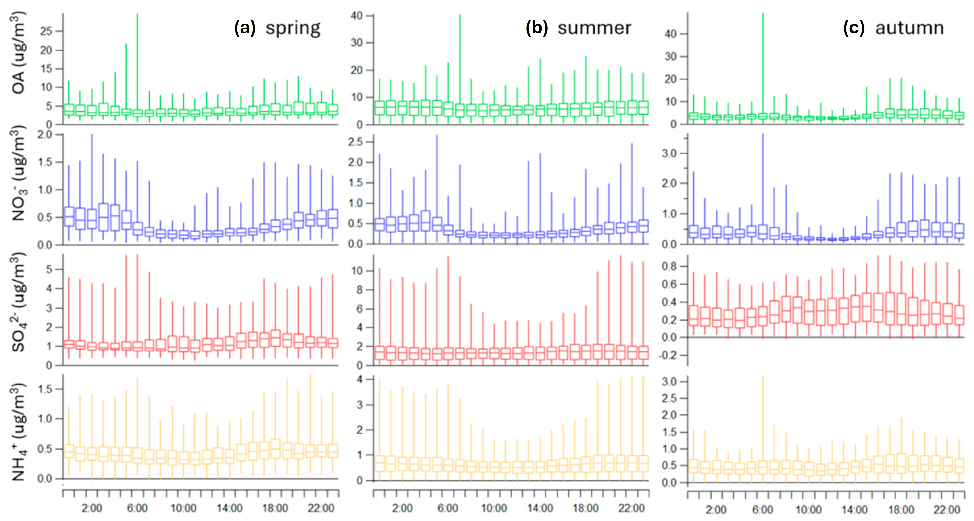
Figure 7 shows the average diurnal behavior calculated for different sub-periods of the dataset, defined according to the astronomical calendar (“spring” from May to 19 June, “summer” from 20 June to 21 September, and “autumn” from 22 September to 31 October). This subdivision was adopted as a temporal framework to organize the data, rather than to represent actual seasonal conditions. It is important to note that only the summer period is fully covered, while the spring and autumn intervals are only partially represented. Therefore, the following analysis is intended to describe temporal variability within the study period rather than to provide a complete characterization of seasonal behavior, given the limited coverage period and the lack of sufficient data to cover all seasons of the year.
As Figure 7 shows, a variability in the daily mean behavior of the chemical species concentrations can be observed when considering the different sub-periods. In the first period (Figure 7a), it can be seen that NH4+ and SO42− show a similar behavior. The interquartile variability is much more pronounced, especially during working hours, which may be due to different emission sources (e.g., industrial or agricultural) and to meteorological conditions (indeed, there was an increase in T). Contrary to what was observed for NH4+ and SO42−, NO3 shows a higher interquartile variability only during the night, suggesting that there are specific factors influencing its concentration predominantly during night-time. An interesting factor that could affect this behavior could be linked to the anthropogenic activities, which can influence the concentration of oxidation reaction precursor’s emissions such as NOx. Temperature inversions can also limit pollutants near the surface, increasing nitrate concentrations and contributing to greater variability. Regarding OA, interquartile range variability is observed at night, with median values shifting toward Q1, indicating a positive skewness. As with NO3, another factor to consider is nocturnal emissions with the secondary formation of organic aerosol through chemical reactions and condensation of organic vapors during the night, which could explain the high variability and the extreme values reached, almost systematically detectable at certain times of the day.
In Figure 7b the diurnal behavior of the different chemical species for the second period are shown. The values are comparable to those in the first period, with some differences concerning NH4+ and SO42−, for which higher but almost constant median values are observed throughout the day. This could indicate the presence of a continuous source of emission, or an equilibrium reached in the atmospheric system during this time. A notable difference is also observed between the maximum values obtained during the night and those during the day, probably due to the different climatic conditions between day and night.
NO3 concentrations do not vary substantially from the first to second period, showing almost comparable behavior and indicating similarities in the formation mechanisms and sources of precursor emissions in the two periods considered. For OA, however, a slight increase in concentrations and interquartile range is observed, likely due to increased biological activity. Finally, Figure 7c shows a decrease in OA and SO42− concentrations in the third period, while NH4+ and NO3 concentrations do not show significant differences. As previously highlighted, the average RH value varied significantly, from 60% in the second period to values above 75% (up to 96%) during the third period. At the same time, both AP and T showed a variation consistent with what can be expected, reporting an increase in precipitation events and a drop in T from 25 °C to 15 °C. The variation in concentrations can, therefore, be attributed to the atmospheric conditions, which may have favored the condensation of species on aqueous particles, resulting in atmospheric washing.
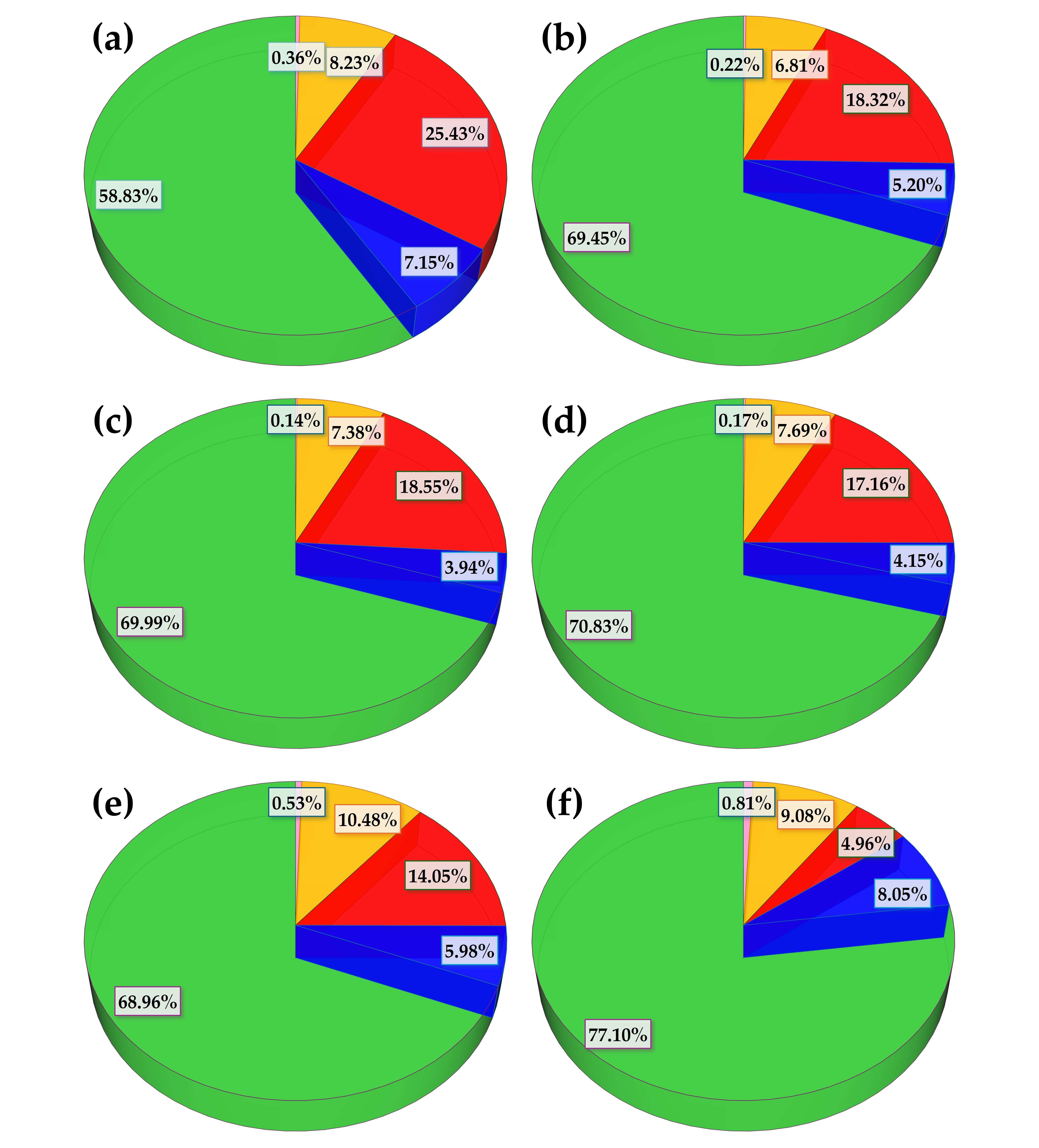
Figure 8 reports the monthly evolution of the percentage contribution of the main chemical species over the six-month observation period. From May to October, although the absolute concentrations of organic compounds decrease, their relative contribution may increase when the concurrent decline of the other species is proportionally larger.
This meteorological variability directly impacts the behavior of different species. For OA, whose absolute concentration is likely reduced due to meteorological variability, its removal is clearly intensified through dissolution equilibria and a decrease in biogenic emissions. Nevertheless, the organic fraction shows an increase compared to the inorganic components.
Regarding SO42−, its percentage contribution is clearly decreasing, falling from 25.43% in May to 4.96% in October, consistent with the reduced photochemical production of sulfates and the intensification of removal processes in late summer and autumn. NO3 shows an opposite trend: its contribution decreases in the warmer month and subsequently increases during the September–October period, rising from 7.15% to 8.05%. This trend is likely due to lower temperatures and, therefore, to a greater distribution of nitrates in the particulate phase. NH4+ remains relatively stable, maintaining values fluctuating around 8.0% throughout the period, with a slight increase starting in September, consistent with its role in neutralizing both sulfate and nitrate. Finally, Cl concentration remains close to the detection limit with a very low percentage concentration; the slight increase observed since September could be associated with increased emissions from combustion sources associated with the restart of home heating systems or changes in the origin of air masses.

3.4. Correlation Analysis

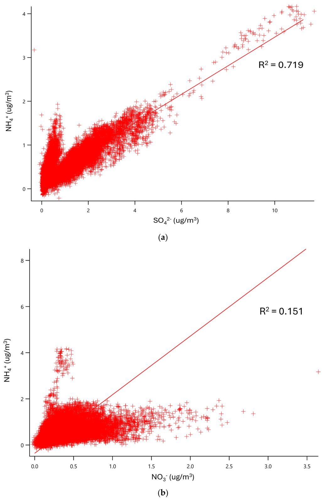
To understand the correlation between inorganic ions, Figure 9 display scatter plots of NH4+ vs. SO42− and NH4+ vs. NO3, presenting concentration values (in µg/m3) obtained throughout the entire analysis period. Subsequently, the R2 value for each scatter plot was calculated and discussed.
Figure 9a shows the correlation obtained (R2 = 0.72) between SO42− and NH4+, suggesting that a significant portion of atmospheric NH4+ combines with SO42− to form ammonium sulfate ((NH4)2SO4). The presence of ammonium sulfate may suggest reactions between ammonia (NH3) emitted by anthropogenic sources (e.g., agriculture, traffic, and industry) with sulfuric acid (H2SO4) derived from the oxidation of sulfur dioxide (SO2).
Figure 9b shows the obtained correlation (R2 = 0.15) between NO3 and NH4+, suggesting that ammonium nitrate (NH4NO3) does not appear to be a dominant or stable component in atmospheric particulate matter.
NO3 could be formed mainly from nitrogen oxides (NOx) through secondary reactions. NOx, originating from sources such as vehicular traffic, power plants, industries, and biomass burning, react in the atmosphere to form nitric acid (HNO3), which can lead to the formation of NO3 [58]. Furthermore, NO3 can be present in the atmosphere in association with various bases and cations present in the environment, such as Na+, K+, Ca2+, and Mg2+. The possible presence of sodium nitrate (NaNO3) can be attributed to reactions with marine aerosols [59], while the possible presence of potassium nitrate (KNO3) can be linked to agricultural sources or soil resuspension. Calcium nitrate (Ca(NO3)2) and magnesium nitrate (Mg(NO3)2), two other possibly present chemical species, are formed through reactions with mineral and crustal particles [60].
Finally, NO3 can be adsorbed onto the surface of atmospheric dust particles from the desert, or it can directly react with volatile organic compounds (VOCs).
All these processes can occur in the area under study since they are affected by both anthropogenic phenomena (vehicular traffic, industrial activities, agricultural activities, and crustal material movement) and natural phenomena also related to long-range transport of air masses (Saharan dust intrusion and potential interaction with marine aerosols). Further studies on the ionic composition of particulate matter using ion chromatography in combination with data obtained using ToF-ACSM will allow for a more accurate study of the chemical composition of particulate matter.

3.5. Acidity of NR-PM1

The study of atmospheric acidity is of fundamental importance for several reasons. It helps in understanding the complex chemical–physical equilibria that regulate heterogeneous reactions, the hygroscopic growth of aerosols, and the overall toxicity of air for both humans and ecosystems. Atmospheric acidity plays a critical role in determining the behavior of pollutants, their transformation, and their impact on health and the environment.
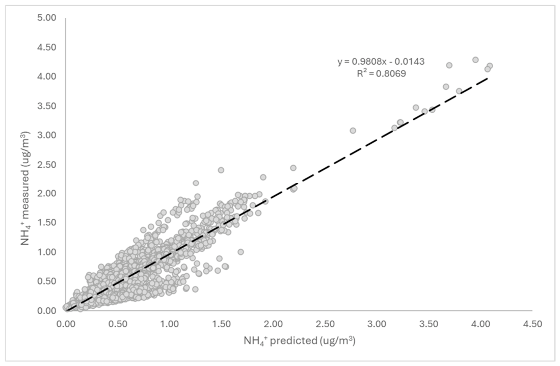
In this work, we focus on the acidity in NR-PM1 by analyzing and comparing the mass concentration (in µg/m3) of NH4+ measured with the mass concentration of NH4+ necessary to neutralize the measured anionic components (SO42−, NO3 and Cl). This comparison allows us to infer the level of acidity and the degree of neutralization of the aerosols. By carrying out the following charge balance, we can determine the extent to which ammonium neutralizes the acidic components.
[NH4+] predict = 18.05 × 2 ([SO4]2−/96.06 + [NO3]/62.01 + [Cl]/35:45),
where [SO4]2−, [NO3], and [Cl] represent the mass concentrations (µg/m3) of the species, 18.05 is the molecular mass of [NH4+] and the denominators correspond to the molecular mass of the anions. It is important to note that this approach considers the contribution of metallic ions and organic acids and bases negligible [61].
Given the characteristics of the site, the most significant contributions can be attributed to ammonium nitrate and ammonium sulfate, whose presence at ground level could be due to vehicular traffic, industrial and agricultural activities. In this context, crustal aerosol, such as calcium sulfate, originating from soil erosion or industrial activities like cement production, should not be excluded. Considering the above-mentioned approximations and to achieve charge neutralization of the system, if the measured [NH4+] concentration is significantly lower than the theoretically expected concentration, the suspended particles will be much more acidic.
Figure 10 illustrates the correlation between predicted and measured NH4+. The R2 value is relatively high (0.81), indicating that there is a good correlation between the variables. PM1 was largely neutralized during this measurement period, although not completely. From the information illustrated above and the concentration temporal behavior discussed in the previous paragraphs, we can conclude that nitrate, not being completely neutralized by ammonium, is present in the atmosphere in other forms, likely as inorganic salts or bound to VOCs.

3.6. Organic Aerosol Components

Organic species are an important component of aerosols at CIAO, with a variation recorded from 58% to 77% during the entire period.
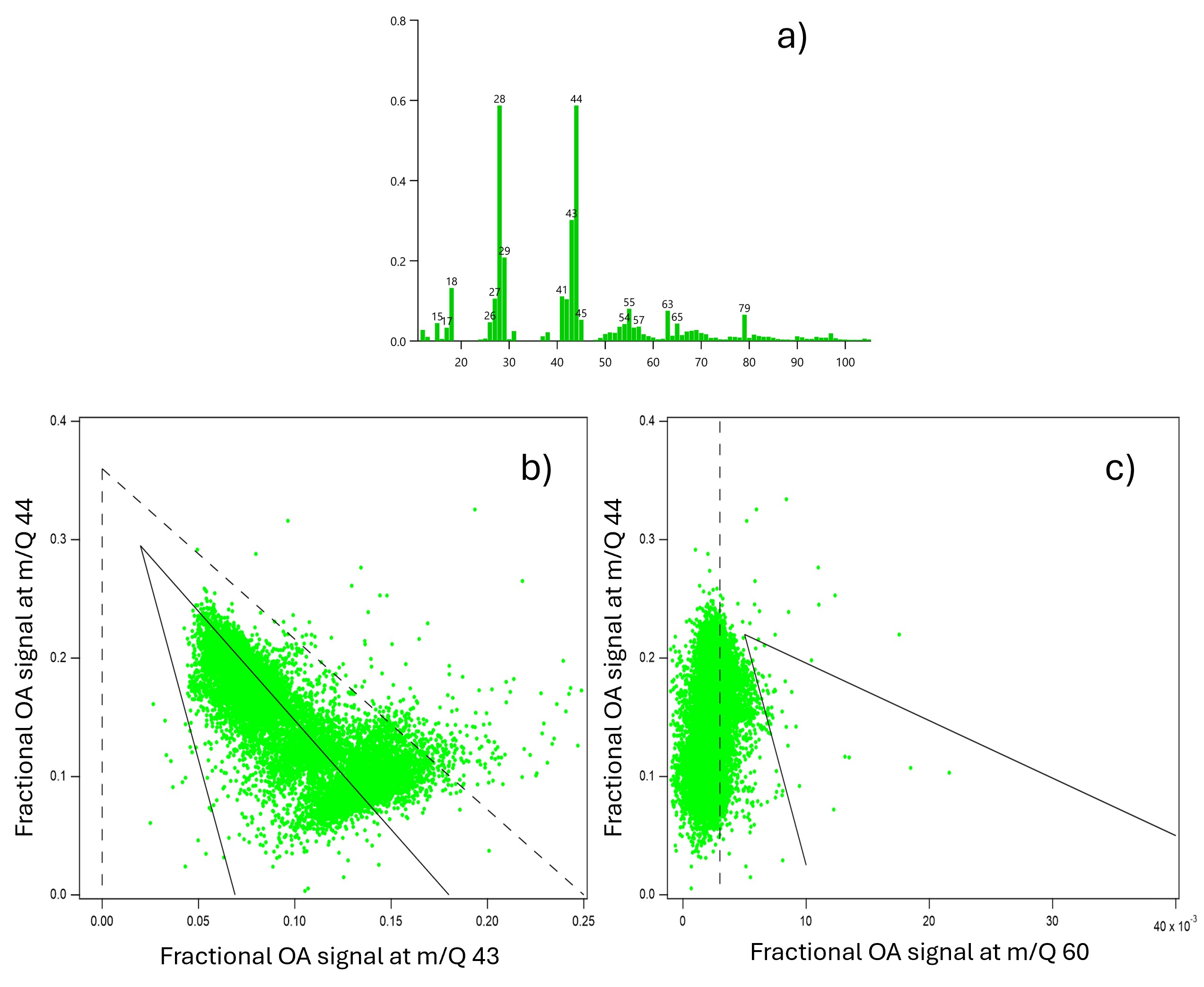
Figure 11a–c shows the mass spectrum related to the organic component for the entire time series, the plot of m/z 44 (f44) vs. m/z 43 (f43) and the plot of m/z 44 vs. m/z 60 (f60), respectively.
From the mass spectrum, the intensity of fragments belonging to both oxygenated organic aerosols (OOA) and hydrocarbon-like organic aerosols (HOA) can be derived for the entire analysis period. From the relative abundance of the peaks, characteristic peaks of hydrocarbon species such as C3H5+ (m/z 41), C3H7+ (m/z 43), C4H7+ (m/z 55), and C4H9+ (m/z 57) are noted to be much less intense compared to other peaks belonging to oxygenated species, such as CO (m/z 28) and CO2 (m/z 44).
In Figure 11b, the plot of f44 vs. f43 is reported, where f44 represents the presence of oxygenated organics that release more CO2+ ions, and f43 represents the presence of hydrocarbon-like organics that release more C3H7+ ions. The solid lines enclose values where ambient OOA components fall [62], while the dotted one encloses values where laboratory experiment components fall [63]. Higher f44 values falling above the dotted line indicate a higher level of oxidation and photochemical aging of the aerosols. The composition of the f44/f43 ratio of ambient OOA can provide information on the oxidation level, composition of different types of organic aerosols and the structures of the chemical precursors that originated them [63].
OOA located towards the left edge of the triangle may be influenced by non-methylated aromatic precursors and/or glyoxal. These precursors tend to generate lower f43 values.
OOA located towards the right edge of the triangle may be influenced by aromatic, biogenic, and/or methylated alkane precursors. These precursors tend to generate higher f43 values. Points outside the typical range can therefore represent unusual chemical compositions potentially influenced by specific chemical precursors and particular environmental conditions.
An example can be represented by aerosols derived from specific sources such as wildfires, specific industrial emissions, or uncommon chemical reactions. Indeed, multiple chemical reactions, combinations of precursors, and specific atmospheric conditions can contribute to the formation of aerosols outside the typical range.
In Figure 11c, the plot of f44 vs. f60 is shown, where f60 represents the presence of biomass burning aerosols that contain anhydro sugars, like levoglucosan, that generate C2H4O2+. In this case as well, the solid lines enclose the area corresponding to ambient observations with known biomass burning [64].
The position of the points towards the dashed line on the left in the f44 vs. f60 plot indicates the absence or a reduced influence of biomass burning. Indeed, measurements that shift towards the dashed line on the left indicate that the aerosols have little to no influence from biomass burning. This is consistent with what is described by [64], where it is observed that with aging, f60 tends to decrease while f44 increases, representing significant photochemical aging without a marked contribution from biomass burning.
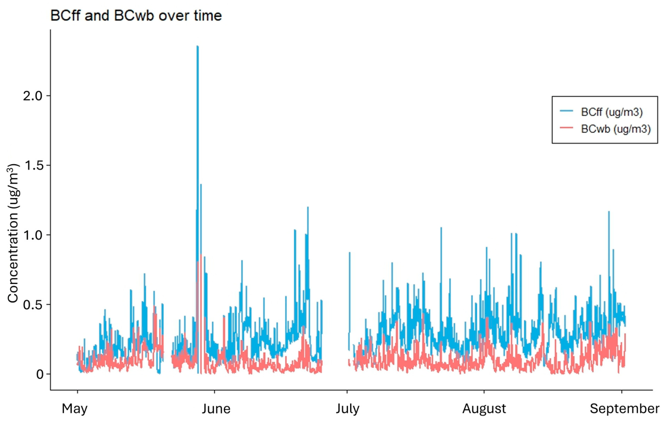
The minimal contribution from biomass burning can be highlighted by Figure 12, which shows the hourly averaged contributions to BC from biomass burning (BCbb, orange) and fossil fuel (BCff, grey) as hourly averages, as measured by the Aethalometer operating with a PM10 inlet.
As can be observed, throughout the entire analysis period, except for specific pollution events, the contribution to BC was predominantly attributable to fossil fuel sources. Despite this, concentration remained low, with maximum values of BCbb and BCff reaching 0.86 μg/m3 and 2.36 μg/m3, respectively.
Although these measurements cover a larger size fraction than the submicron aerosol analyzed by TOF-ACSM, integrating these data with future collections will allow exploration of local and non-local aerosol sources impacting the observatory. This approach will be further enhanced by planned offline chemical analyses of the collected filters, including multi-wavelength thermal/optical carbon analysis and gas chromatography–mass spectrometry (GC-MS), which will allow for a more detailed characterization of the organic compounds and their sources.

3.7. Comparison with Other ACTRIS Observation Sites

One of the most important features of the research infrastructure is its ability to provide the community with data acquired using the same instrumentation and adopting the same measurement protocols to obtain comparable data.
To study the similarities and differences between different observation sites, the percentage contribution of the different fractions obtained from the same analysis period, although from different years, was compared (Figure 13). All data were taken from the EBAS data archive (https://ebas-data.nilu.no/, accessed on 1 July 2025) and were subsequently used to obtain data reported in Table 2.

Table 2 reports information on the percentage concentrations of the five chemical species for 11 ACTRIS observation sites. Each site has a specific percentage of each of these chemical species, reflecting the air quality in that area. Figure 14 shows the spider diagrams for all the observation stations considered where it is possible to visualize all the fractions reported in Table 2.
From the different spider diagrams, it can be seen that (OA) constitutes a significant part of the aerosol composition at all stations, with values ranging from approximately ≈70% to ≈87%. Despite this notable difference, comparing the five chemical species allows us to study the variability between different sites and to establish three distinct compositional profiles. The first profile is characterized by a clear prevalence of organic compounds, with concentration levels of approximately 87%. Inorganic contributions are low; in fact, Jungfraujoch (OA = 86.71%, SO4 = 3.99%, NO3 = 2.44%) and Kosetice (OA = 85.86%, NO3 = 1.62%) are typical examples where the inorganic fraction is remarkably low. The second profile presents more balanced concentrations, with OA generally close to 80% and moderate SO42− and NO3 values, such as those observed at the SIRTA (OA = 79.10%, NO3 = 3.27%, SO4 = 7.37%), Birkenes (OA = 81.87%, SO4 = 5.22%), and Melpitz (OA = 80.04%, NO3 = 3.37%, SO4 = 8.37%). The third profile shows a decrease in the organic component (approximately 75%) together with an increase in the inorganic component, particularly sulfates and nitrates. CIAO (OA = 70.21%, SO4 = 16.22%, NO3 = 5.17%) and Athens DEM (OA = 74.79%, SO4 = 13.08%) show a marked trend, while Barcelona (OA = 73.07%, SO4 = 14.33%) and ISAC Bologna (OA = = 77.25%, NO3 = 3.31%) show a greater presence of the inorganic fraction compared to the sites of the first and second profiles. Within these profiles, some stations show characteristics that suggest hybrid behavior. CIAO stands out about its inorganic component, having the highest relative contributions of SO42− (16.22%) and NO3 (5.17%). This finding indicates that secondary inorganic species play a significant role compared to the organic component. University College Dublin combines the relatively low OA value (71.38%) with the highest chloride value (1.81%); to these, the high ammonium value (12.81%) is added, creating a distinctive profile compared to the other stations. Chloride concentration, although small in absolute terms, still appears significant enough to influence the differences between the observation sites. Melpitz, with intermediate OA values (80.04%), also shows notable contributions from NO3 and SO42− (3.37% and 8.37% respectively), indicating an intermediate behavior between the first and second profiles. Similarly, Milano Pascal (OA = 76.34%) shows one of the highest NO3 concentration values (3.98%), suggesting a greater presence of nitrates compared to other sites with similar OA concentrations. Finally, Table 2 supports the idea that the variations between the various profiles lie in the different balance between OA and SO42−//NO3, with NH4+ and Cl offering further insights into the climate at the local, strictly, and regional levels.

4. Conclusions

A six-month study was conducted at the CIAO between May and October 2024, providing an initial characterization of the chemical composition and variability of NR PM1. The study allowed us to exploratorily analyze the chemical species trends at the observation site, influenced by meteorological conditions and local emission sources. Specifically, traffic-related emissions contributed minimally to black carbon (BC) concentrations, while organic aerosol, sulphate and nitrate concentrations showed unique daily trends, highlighting the combined role of primary emissions deriving from different sources and atmospheric processes.
The behavior of inorganic species confirmed some of the chemical interactions present in the literature and allowed for the formulation of hypotheses that will require further data to be confirmed. The high correlation between NH4+ and SO42− (R2 = 0.80) indicates efficient ammonium sulfate formation through the reaction of NH3 with H2SO4. PM1 neutralization occurs largely thanks to the ammonium present, although additional acidic species likely contribute to the formation and partitioning of nitrates. It is important to note that other species, both organic and inorganic, also contribute to PM1 neutralization, and this aspect will be explored further in future studies.
The organic fraction represents a significant portion of the total NR-PM1 mass. To obtain an initial exploratory analysis, specific signals at different m/z ratios were compared. This allowed us to distinguish between oxygenated and non-oxygenated organic aerosols, assess the degree of aging, and formulate hypotheses regarding the nature of the precursors and sources. Indeed, the results highlighted a clear prevalence of oxidized organic compounds, indicative of significant atmospheric processing that will be further explored in future studies.
The comparative analysis of the chemical profiles of the different sites allowed us to define different compositional profiles. One profile is characterized by a clear prevalence of organic compounds, indicative of remote stations not significantly affected by urban pollution. Another profile exhibits the opposite characteristics, characterized by a decrease in the organic fraction (up to approximately 15%) and an increase in inorganic components. Finally, what appears to be an intermediate profile was observed, with the organic fraction reaching 80%. Given the complexity of these comparisons between different observation stations, it will be essential to collect significantly more chemical data to better understand the influence of local and global phenomena.
Finally, these results highlight the complexity of organic and inorganic processes affecting local air quality and demonstrate the ability of ToF-ACSM to provide real-time information on aerosol composition. The information collected across multiple variables can provide a valuable source of information for better understanding the mechanisms governing aerosol formation and transformation at both the local and regional scales.
Although this work represents first exploration analysis based on a limited observation period, it sets the starting point for more detailed investigations of the atmospheric processes affecting the study area, which can be integrated with other OSs within ACTRIS. Future activities will include chemical characterization (via Multi-Wavelength Thermal/Optical Carbon Analyzer, Ion Chromatography, Induced Coupled Plasma-Optical Emission Spectroscopy, Gas Chromatography–Mass Spectrometry) of PM1, PM2.5, and PM10 samples collected on quartz and Teflon filters, as well as the application of positive matrix factorization to the resulting datasets to identify sources and understand secondary formation pathways. Further attention will be paid to the presence of Saharan dust intrusions in the observation site area, which further highlights the complexity of aerosol dynamics and the need to compare both natural and anthropogenic contributions.
Finally, within ACTRIS, the instrument’s participation in the ECAC interlaboratory comparison at the ACTRIS Aerosol Chemical Monitor Calibration Center in 2025 has ensured data reliability and strengthened the integration of CIAO within the infrastructure, ensuring better long-term comparability of datasets.

Author Contributions

Conceptualization, F.C.; methodology, F.C.; software, F.C. and E.L.; validation, F.C.; formal analysis, F.C.; investigation, F.C.; resources, D.A., C.C. and E.L.; data curation, F.C., T.L. and E.L.; writing—original draft preparation, F.C.; writing—review and editing, F.C., T.L., E.L., D.A., C.C., A.B., I.Z., G.D.F., S.T. and L.M.; visualization, F.C., T.L. and E.L.; supervision, S.T. and L.M.; project administration and funding acquisition, L.M., S.T. and G.D.F. All authors have read and agreed to the published version of the manuscript.

Funding

This research was funded by MUR (Italian Ministry of University and Research) under the following projects: PER-ACTRIS-IT (Potenziamento della componente italiana della Infrastruttura di Ricerca Aerosol, Clouds, and Trace Gases Research Infrastructure), COD. PIR01_00015, CUP B17E19000000007-PON “Ricerca e Innovazione 2014–2020” Avviso MUR D.D. n. 424 del 28 February 2018, CIR01_00015 PER-ACTRIS-IT (strengthening human capital)-Avviso MUR D.D. n. 2595 del 24 December 2019 Piano Stralcio “Ricerca e Innovazione 2015–2017”, CUP B58I20000220001, CIR01_00019 PRO ICOS MED (Potenziamento della Rete di Osservazione ICOS-Italia nel Mediterraneo—Rafforzamento del capitale umano)—Avviso MUR D.D. n. 2595 del 24 December 2019 Piano Stralcio “Ricerca e Innovazione 2015–2017”, CUP B58I20000210001, ITINERIS, Italian Integrated Environmental Research Infrastructure System (IR0000032, D.D. n.130/2022—CUPB53C22002150006) Funded by EU—Next Generation EU PNRR—Mission 4—Component 2—Investment 3.1, and the Joint Research Unit ACTRIS Italy, Ordinary Fund for Research Institutions and Organizations (FOE) 2024, funded by the Italian Ministry of University and Research (D.M. n. 1096, 25 July 2024).

Institutional Review Board Statement

Not applicable.

Informed Consent Statement

Not applicable.

Data Availability Statement

The dataset is available via the ITINERIS HUB: https://doi.org/10.71763/ITINERIS-HUB/YKVE-CA78, accessed on 1 July 2026.

Acknowledgments

This work has been supported by the ACTRIS research infrastructure, and the authors gratefully acknowledge the contributions of the Center for Aerosol In-Situ-European Cen-ter for Aerosol Calibration and Characterization (CAIS-ECAC) in ensuring data quality, harmonization, and traceability.

Conflicts of Interest

The authors declare no conflicts of interest.

References

  1. IPCC. Sections. In Climate Change 2023: Synthesis Report. Contribution of Working Groups I, II and III to the Sixth Assessment Report of the Intergovernmental Panel on Climate Change; Core Writing Team, Lee, H., Romero, J., Eds.; IPCC: Geneva, Switzerland, 2023; pp. 35–115. [Google Scholar] [CrossRef]
  2. Li, J.; Carlson, B.E.; Yung, Y.L.; Lv, D.; Hansen, J.; Penner, J.E.; Liao, H.; Ramaswamy, V.; Kahn, R.A.; Zhang, P.; et al. Scattering and absorbing aerosols in the climate system. Nat. Rev. Earth Environ. 2022, 3, 363–379. [Google Scholar] [CrossRef]
  3. Tao, W.-K.; Chen, J.-P.; Li, Z.; Wang, C.; Zhang, C. Impact of aerosols on convective clouds and precipitation. Rev. Geophys. 2012, 50, RG2001. [Google Scholar] [CrossRef]
  4. Ramanathan, V.; Crutzen, P.J.; Kiehl, J.T.; Rosenfeld, D. Aerosols, Climate, and the Hydrological Cycle. Science 2001, 294, 2119–2124. [Google Scholar] [CrossRef] [PubMed]
  5. Charlson, R.J.; Schwartz, S.E.; Hales, J.M.; Cess, R.D.; Coakle, J.A., Jr.; Hansen, J.E.; Hofmann, D.J. Climate forcing by anthropogenic aerosols. Science 1992, 255, 423–430. [Google Scholar] [CrossRef] [PubMed]
  6. Guo, J.; Miao, Y.; Zhang, Y.; Liu, H.; Li, Z.; Zhang, W.; He, J.; Lou, M.; Yan, Y.; Bian, L.; et al. The climatology of planetary boundary layer height in China derived from radiosonde and reanalysis data. Atmos. Chem. Phys. 2016, 16, 13309–13319. [Google Scholar] [CrossRef]
  7. Twomey, S.A.; Piepgrass, M.; Wolfe, T.L. An assessment of the impact of pollution on global cloud albedo. Tellus B Chem. Phys. Meteorol. 1984, 36, 356–366. [Google Scholar] [CrossRef]
  8. Li, B.; Gasser, T.; Ciais, P.; Piao, S.; Tao, S.; Balkanski, Y.; Hauglustaine, D.; Boisier, J.P.; Chen, Z.; Huang, M.; et al. The contribution of China’s emissions to global climate forcing. Nature 2016, 531, 357–361. [Google Scholar] [CrossRef] [PubMed]
  9. Li, Q.; Zhang, C.; Shen, Y.; Jia, W.; Li, J. Quantitative assessment of the relative roles of climate change and human activities in desertification processes on the Qinghai-Tibet Plateau based on net primary productivity. Catena 2016, 147, 789–796. [Google Scholar] [CrossRef]
  10. Pan, X.; Kanaya, Y.; Taketani, F.; Miyakawa, T.; Inomata, S.; Komazaki, Y.; Tanimoto, H.; Wang, Z.; Uno, I.; Wang, Z. Emission characteristics of refractory black carbon aerosols from fresh biomass burning: A perspective from laboratory experiments. Atmos. Chem. Phys. 2017, 17, 13001–13016. [Google Scholar] [CrossRef]
  11. Pan, X.; Uno, I.; Wang, Z.; Nishizawa, T.; Sugimoto, N.; Yamamoto, S.; Kobayashi, H.; Sun, Y.; Fu, P.; Tang, X.; et al. Real-time observational evidence of changing Asian dust morphology with the mixing of heavy anthropogenic pollution. Sci. Rep. 2017, 7, 335. [Google Scholar] [CrossRef] [PubMed]
  12. Sun, Y.L.; Wang, Z.F.; Du, W.; Zhang, Q.; Wang, Q.Q.; Fu, P.Q.; Pan, X.L.; Li, J.; Jayne, J.; Worsnop, D.R. Long-term real-time measurements of aerosol particle composition in Beijing, China: Seasonal variations, meteorological effects, and source analysis. Atmos. Chem. Phys. 2015, 15, 10149–10165. [Google Scholar] [CrossRef]
  13. Feng, Z.; Leung, L.; Hagos, S.; Houze, R.A.; Burleyson, C.D.; Balaguru, K. More frequent intense and long-lived storms dominate the springtime trend in central US rainfall. Nat. Commun. 2016, 7, 13429. [Google Scholar] [CrossRef] [PubMed]
  14. Pope, C.A., 3rd; Dockery, D.W. Health effects of fine particulate air pollution: Lines that connect. J. Air Waste Manag. Assoc. 2006, 56, 709–742. [Google Scholar] [CrossRef] [PubMed]
  15. Shiraiwa, M.; Ueda, K.; Pozzer, A.; Lammel, G.; Kampf, C.J.; Fushimi, A.; Enami, S.; Arangio, A.M.; Fröhlich-Nowoisky, J.; Fujitani, Y.; et al. Aerosol Health Effects from Molecular to Global Scales. Environ. Sci. Technol. 2017, 51, 13545–13567. [Google Scholar] [CrossRef] [PubMed]
  16. Arfin, T.; Pillai, A.M.; Mathew, N.; Tirpude, A.; Bang, R.; Mondal, P. An overview of atmospheric aerosol and their effects on human health. Environ. Sci. Pollut. Res. 2023, 30, 125347–125369. [Google Scholar] [CrossRef] [PubMed]
  17. Damiati, S.; AlMashrea, B.A.; Rabiei, N.; Sujatha, A.P.; Sabir, D.K.; Alhosani, M.; Kodzius, R. Aerosol Pollutants and Health: Role of Size and Chemical Composition. Public Health Chall. 2025, 4, E70134. [Google Scholar] [CrossRef] [PubMed]
  18. Goshua, A.; Akdis, C.A.; Nadeau, K.C. World Health Organization global air quality guideline recommendations: Executive summary. Allergy 2022, 77, 1955–1960. [Google Scholar] [CrossRef] [PubMed]
  19. Lelieveld, J.; Pozzer, A.; Pöschl, U.; Fnais, M.; Haines, A.; Münzel, T. Loss of life expectancy from air pollution compared to other risk factors: A worldwide perspective. Cardiovasc. Res. 2020, 116, 1910–1917. [Google Scholar] [CrossRef] [PubMed]
  20. Ibald-Mulli, A.; Wichmann, H.E.; Kreyling, W.; Peters, A. Epidemiological evidence on health effects of ultrafine particles. J. Aerosol Med. 2002, 15, 189–201. [Google Scholar] [CrossRef] [PubMed]
  21. Kreyling, W.G.; Semmler-Behnke, M.; Möller, W. Ultrafine particle-lung interactions: Does size matter? J. Aerosol Med. 2006, 19, 74–83. [Google Scholar] [CrossRef] [PubMed]
  22. Elser, M.; Huang, R.J.; Wolf, R.; Slowik, J.G.; Wang, Q.; Canonaco, F.; Li, G.; Bozzetti, C.; Daellenbach, K.R.; Huang, Y.; et al. New insights into PM2.5 chemical composition and sources in two major cities in China during extreme haze events using aerosol mass spectrometry. Atmos. Chem. Phys. 2016, 16, 3207–3225. [Google Scholar] [CrossRef]
  23. Chaturvedi, S.; Kumar, A.; Singh, V.; Chakraborty, B.; Kumar, R.; Min, L. Recent Advancement in Organic Aerosol Understanding: A Review of Their Sources, Formation, and Health Impacts. Water Air Soil. Pollut. 2023, 234, 750. [Google Scholar] [CrossRef]
  24. Zhao, X.; Ma, X.; Chen, B.; Shang, Y.; Song, M. Challenges toward carbon neutrality in China: Strategies and countermeasures. Resour. Conserv. Recycl. 2022, 176, 105959. [Google Scholar] [CrossRef]
  25. Kuang, Y.; He, Y.; Xu, W.; Yuan, B.; Zhang, G.; Ma, Z.; Wu, C.; Wang, C.; Wang, S.; Zhang, S.; et al. Photochemical Aqueous-Phase Reactions Induce Rapid Daytime Formation of Oxygenated Organic Aerosol on the North China Plain. Environ. Sci. Technol. 2020, 54, 3849–3860. [Google Scholar] [CrossRef] [PubMed]
  26. Wang, S.; Zhang, J.; Zhang, Y.; Wang, L.; Sun, Z.; Wang, H. Review on Source Profiles of Volatile Organic Compounds (VOCs) in Typical Industries in China. Atmosphere 2023, 14, 878. [Google Scholar] [CrossRef]
  27. Aiken, A.C.; Salcedo, D.; Cubison, M.J.; Huffman, J.A.; DeCarlo, P.F.; Ulbrich, I.M.; Docherty, K.S.; Sueper, D.; Kimmel, J.R.; Worsnop, D.R.; et al. Mexico City aerosol analysis during MILAGRO using high resolution aerosol mass spectrometry at the urban supersite (T0)—Part 1: Fine particle composition and organic source apportionment. Atmos. Chem. Phys. 2009, 9, 6633–6653. [Google Scholar] [CrossRef]
  28. Zhang, Q.; Jimenez, J.L.; Canagaratna, M.R.; Ulbrich, I.M.; Ng, N.L.; Worsnop, D.R.; Sun, Y. Understanding atmospheric organic aerosols via factor analysis of aerosol mass spectrometry: A review. Anal. Bioanal. Chem. 2011, 401, 3045–3067. [Google Scholar] [CrossRef] [PubMed]
  29. Sun, Y.L.; Wang, Z.F.; Fu, P.Q.; Yang, T.; Jiang, Q.; Dong, H.B.; Li, J.; Jia, J.J. Aerosol composition, sources and processes during wintertime in Beijing, China. Atmos. Chem. Phys. 2013, 13, 4577–4592. [Google Scholar] [CrossRef]
  30. Crippa, M.; El Haddad, I.; Slowik, J.G.; DeCarlo, P.F.; Mohr, C.; Heringa, M.F.; Chirico, R.; Marchand, N.; Sciare, J.; Baltensperger, U.; et al. Identification of marine and continental aerosol sources in Paris using high resolution aerosol mass spectrometry. J. Geophys. Res. Atmos. 2013, 118, 1950–1963. [Google Scholar] [CrossRef]
  31. Lee, T.; Choi, J.; Lee, G.; Ahn, J.; Park, J.S.; Atwood, S.A.; Schurman, M.; Choi, Y.; Chung, Y.; Collett, J.L., Jr. Characterization of aerosol composition, concentrations, and sources at Baengnyeong Island, Korea using an aerosol mass spectrometer. Atmos. Environ. 2015, 120, 297–306. [Google Scholar] [CrossRef]
  32. De Carlo, P.F.; Kimmel, J.R.; Trimborn, A.; Northway, M.J.; Jayne, J.T.; Aiken, A.C.; Gonin, M.; Fuhrer, K.; Horvath, T.; Docherty, K.S.; et al. Field-deployable, high-resolution, time-of-flight aerosol mass spectrometer. Anal. Chem. 2006, 78, 8281–8289. [Google Scholar] [CrossRef] [PubMed]
  33. Canagaratna, M.R.; Jayne, J.T.; Jimenez, J.L.; Allan, J.D.; Alfarra, M.R.; Zhang, Q.; Onasch, T.B.; Drewnick, F.; Coe, H.; Middlebrook, A.; et al. Chemical and microphysical characterization of ambient aerosols with the aerodyne aerosol mass spectrometer. Mass. Spectrom. Rev. 2007, 26, 185–222. [Google Scholar] [CrossRef] [PubMed]
  34. The Aerosol, Clouds and Trace Gases Research Infrastructure. Available online: https://actris.eu/ (accessed on 1 July 2025).
  35. Laj, P.; Lund Myhre, C.; Riffault, V.; Amiridis, V.; Fuchs, H.; Eleftheriadis, K.; Petäjä, T.; Salameh, T.; Kivekäs, N.; Juurola, E.; et al. Aerosol, clouds and trace gases research infrastructure (ACTRIS): The European research infrastructure supporting atmospheric science. Bull. Am. Meteorol. Soc. 2024, 105, E1098–E1136. [Google Scholar] [CrossRef]
  36. Laurita, T.; Mauceri, A.; Cardellicchio, F.; Lapenna, E.; De Rosa, B.; Trippetta, S.; Mytilinaios, M.; Amodio, D.; Giunta, A.; Ripepi, E.; et al. CIAO main upgrade: Building up an ACTRIS-compliant aerosol in situ laboratory. Atmos. Meas. Tech. 2025, 18, 2373–2396. [Google Scholar] [CrossRef]
  37. Mona, L.; Amodeo, A.; Pandolfi, M.; Pappalardo, G. Saharan dust intrusions in the Mediterranean area: Three years of Raman lidar measurements. J. Geophys. Res. 2006, 111, D16203. [Google Scholar] [CrossRef]
  38. Soupiona, O.; Papayannis, A.; Kokkalis, P.; Foskinis, R.; Sánchez Hernández, G.; Ortiz-Amezcua, P.; Mylonaki, M.; Papanikolaou, C.-A.; Papagiannopoulos, N.; Samaras, S.; et al. EARLINET observations of Saharan dust intrusions over the northern Mediterranean region (2014–2017): Properties and impact on radiative forcing. Atmos. Chem. Phys. 2020, 20, 15147–15166. [Google Scholar] [CrossRef]
  39. Papanikolaou, C.-A.; Papayannis, A.; Gidarakou, M.; Abdullaev, S.F.; Ajtai, N.; Baars, H.; Balis, D.; Bortoli, D.; Bravo-Aranda, J.A.; Collaud-Coen, M.; et al. Large-Scale Network-Based Observations of a Saharan Dust Event across the European Continent in Spring 2022. Remote Sens. 2024, 16, 3350. [Google Scholar] [CrossRef]
  40. De Rosa, B.; Mytilinaios, M.; Amodeo, A.; Colangelo, C.; D’Amico, G.; Dema, C.; Gandolfi, I.; Giunta, A.; Gumà-Claramunt, P.; Laurita, T.; et al. Observations of Saharan Dust Intrusions over Potenza, Southern Italy, During 13 Years of Lidar Measurements: Seasonal Variability of Optical Properties and Radiative Impact. Remote Sens. 2025, 17, 453. [Google Scholar] [CrossRef]
  41. Buono, A.; Zaccardo, I.; D’Amico, F.; Lapenna, E.; Cardellicchio, F.; Laurita, T.; Amodio, D.; Colangelo, C.; Di Fiore, G.; Giunta, A.; et al. Expanding Continuous Carbon Isotope Measurements of CO2 and CH4 in the Italian ICOS Atmospheric Consortium: First Results from the Continental POT Station in Potenza (Basilicata). Atmosphere 2025, 16, 951. [Google Scholar] [CrossRef]
  42. Pappalardo, G.; Amodeo, A.; Mona, L.; Pandolfi, M.; Pergola, N.; Cuomo, V. Raman lidar observations of aerosol emitted during the 2002 Etna eruption. Geophys. Res. Lett. 2004, 31, L05120. [Google Scholar] [CrossRef]
  43. Pappalardo, G.; Amodeo, A.; Ansmann, A.; Apituley, A.; Arboledas, L.A.; Balis, D.; Böckmann, C.; Chaikovsky, A.; Comeron, A.; D’Amico, G.; et al. EARLINET observations of the Eyjafjallajökull ash plume over Europe. In Lidar Technologies, Techniques, and Measurements for Atmospheric Remote Sensing VI; SPIE: Bellingham, DC, USA, 2010; Volume 7832, pp. 128–136. [Google Scholar] [CrossRef]
  44. Mona, L.; Amodeo, A.; D’Amico, G.; Giunta, A.; Madonna, F.; Pappalardo, G. Multi-wavelength Raman lidar observations of the Eyjafjallajökull volcanic cloud over Potenza, southern Italy. Atmos. Chem. Phys. 2012, 12, 2229–2244. [Google Scholar] [CrossRef]
  45. Pappalardo, G.; Mona, L.; D’Amico, G.; Wandinger, U.; Adam, M.; Amodeo, A.; Ansmann, A.; Apituley, A.; Alados Arboledas, L.; Balis, D.; et al. Four-dimensional distribution of the 2010 Eyjafjallajökull volcanic cloud over Europe observed by EARLINET. Atmos. Chem. Phys. 2013, 13, 4429–4450. [Google Scholar] [CrossRef]
  46. De Rosa, B.; Amato, F.; Amodeo, A.; D’Amico, G.; Dema, C.; Falconieri, A.; Giunta, A.; Gumà-Claramunt, P.; Kampouri, A.; Solomos, S.; et al. Characterization of Extremely Fresh Biomass Burning Aerosol by Means of Lidar Observations. Remote Sens. 2022, 14, 4984. [Google Scholar] [CrossRef]
  47. De Rosa, B.; Amodeo, A.; D’Amico, G.; Papagiannopoulos, N.; Rosoldi, M.; Veselovskii, I.; Cardellicchio, F.; Falconieri, A.; Gumà-Claramunt, P.; Laurita, T.; et al. Characterization of Fresh and Aged Smoke Particles Simultaneously Observed with an ACTRIS Multi-Wavelength Raman Lidar in Potenza, Italy. Remote Sens. 2025, 17, 2538. [Google Scholar] [CrossRef]
  48. Ng, N.L.; Herndon, S.C.; Trimborn, A.; Canagaratna, M.R.; Croteau, P.L.; Onasch, T.B.; Sueper, D.; Worsnop, D.R.; Zhang, Q.; Sun, Y.L.; et al. An Aerosol Chemical Speciation Monitor (ACSM) for Routine Monitoring of the Composition and Mass Concentrations of Ambient Aerosol. Aerosol Sci. Technol. 2011, 45, 780–794. [Google Scholar] [CrossRef]
  49. Fröhlich, R.; Cubison, M.J.; Slowik, J.G.; Bukowiecki, N.; Prévôt, A.S.H.; Baltensperger, U.; Schneider, J.; Kimmel, J.R.; Gonin, M.; Rohner, U.; et al. The ToF-ACSM: A portable aerosol chemical speciation monitor with TOFMS detection. Atmos. Meas. Tech. 2013, 6, 3225–3241. [Google Scholar] [CrossRef]
  50. Jayne, J.T.; Leard, D.C.; Zhang, X.; Davidovits, P.; Smith, K.A.; Kolb, C.E.; Worsnop, D.R. Development of an Aerosol Mass Spectrometer for Size and Composition Analysis of Submicron Particles. Aerosol Sci. Technol. 2000, 33, 49–70. [Google Scholar] [CrossRef]
  51. Xu, W.; Croteau, P.; Williams, L.; Canagaratna, M.; Onasch, T.; Cross, E.; Zhang, X.; Robinson, W.; Worsnop, D.; Jayne, J. Laboratory characterization of an aerosol chemical speciation monitor with PM2.5 measurement capability. Aerosol Sci. Technol. 2017, 51, 69–83. [Google Scholar] [CrossRef]
  52. Middlebrook, A.M.; Bahreini, R.; Jimenez, J.L.; Canagaratna, M.R. Evaluation of composition-dependent collection efficiencies for the Aerodyne aerosol mass spectrometer using field data. Aerosol Sci. Technol. 2012, 46, 258–271. [Google Scholar] [CrossRef]
  53. Canagaratna, M.R.; Jimenez, J.L.; Kroll, J.H.; Chen, Q.; Kessler, S.H.; Massoli, P.; Hildebrandt Ruiz, L.; Fortner, E.; Williams, L.R.; Wilson, K.R.; et al. Elemental ratio measurements of organic compounds using aerosol mass spectrometry: Characterization, improved calibration, and implications. Atmos. Chem. Phys. 2015, 15, 253–272. [Google Scholar] [CrossRef]
  54. Sandradewi, J.; Prévôt, A.S.; Weingartner, E.; Schmidhauser, R.; Gysel, M.; Baltensperger, U. A study of wood burning and traffic aerosols in an Alpine valley using a multi-wavelength Aethalometer. Atmos. Environ. 2008, 42, 101–112. [Google Scholar] [CrossRef]
  55. Day, D.E.; Hand, J.L.; Carrico, C.M.; Engling, G.; Malm, W.C. Humidification factors from laboratory studies of fresh smoke from biomass fuels. J. Geophys. Res. Atmos. 2006, 111, D22202. [Google Scholar] [CrossRef]
  56. Drinovec, L.; Močnik, G.; Zotter, P.; Prévôt, A.S.H.; Ruckstuhl, C.; Coz, E.; Rupakheti, M.; Sciare, J.; Müller, T.; Wiedensohler, A.; et al. The “dual-spot” Aethalometer: An improved measurement of aerosol black carbon with real-time loading compensation. Atmos. Meas. Tech. 2015, 8, 1965–1979. [Google Scholar] [CrossRef]
  57. De Miranda, R.M.; Perez-Martinez, P.J.; De Fatima Andrade, M.; Ribeiro, F.N.D. Relationship between black carbon (BC) and heavy traffic in São Paulo, Brazil. Transp. Res. Part D Transp. Environ. 2019, 68, 84–98. [Google Scholar] [CrossRef]
  58. Theodorakidou, M.; Lambrou, G.I. Public health issues from the exposure to nitrogen oxides: A brief review. ARC J. Public Health Community Med. 2017, 2, 44–56. [Google Scholar] [CrossRef]
  59. Hoffman, R.C.; Laskin, A.; Finlayson-Pitts, B.J. Sodium nitrate particles: Physical and chemical properties during hydration and dehydration, and implications for aged sea salt aerosols. J. Aerosol Sci. 2004, 35, 869–887. [Google Scholar] [CrossRef]
  60. Xu, M.; Tang, C.Y.; Jubb, A.M.; Chen, X.; Allen, H.C. Nitrate Anions and Ion Pairing at the Air-Aqueous Interface. J. Phys. Chem. C 2008, 113, 2082–2087. [Google Scholar] [CrossRef]
  61. Zhang, Q.; Jimenez, J.L.; Worsnop, D.R.; Canagaratna, M. A case study of urban particle acidity and its influence on secondary organic aerosol. Environ. Sci. Technol. 2007, 41, 3213–3219. [Google Scholar] [CrossRef] [PubMed]
  62. Ng, N.L.; Canagaratna, M.R.; Zhang, Q.; Jimenez, J.L.; Tian, J.; Ulbrich, I.M.; Kroll, J.H.; Docherty, K.S.; Chhabra, P.S.; Bahreini, R.; et al. Organic aerosol components observed in Northern Hemispheric datasets from Aerosol Mass Spectrometry. Atmos. Chem. Phys. 2010, 10, 4625–4641. [Google Scholar] [CrossRef]
  63. Lambe, A.T.; Onasch, T.B.; Massoli, P.; Croasdale, D.R.; Wright, J.P.; Ahern, A.T.; Williams, L.R.; Worsnop, D.R.; Brune, W.H.; Davidovits, P. Laboratory studies of the chemical composition and cloud condensation nuclei (CCN) activity of secondary organic aerosol (SOA) and oxidized primary organic aerosol (OPOA). Atmos. Chem. Phys. 2011, 11, 8913–8928. [Google Scholar] [CrossRef]
  64. Cubison, M.J.; Ortega, A.M.; Hayes, P.L.; Farmer, D.K.; Day, D.; Lechner, M.J.; Brune, W.H.; Apel, E.; Diskin, G.S.; Fisher, J.A.; et al. Effects of aging on organic aerosol from open biomass burning smoke in aircraft and laboratory studies. Atmos. Chem. Phys. 2011, 11, 12049–12064. [Google Scholar] [CrossRef]
Figure 1. Location of the CNR-IMAA Atmospheric Observatory (© Google Maps).
Atmosphere 17 00677 g001
Figure 2. Time series of the mass concentrations of organics (Org), nitrate (NO3), sulphate (SO4) and ammonium (NH4) recorded by ToF-ACSM at CIAO from 13 May to 31 October 2024. Chloride mass concentrations are not reported since they are mostly below the limit of detection (LoD).
Atmosphere 17 00677 g002
Figure 3. Diurnal trend of the BC 1 h average concentration during the period May–August 2024.
Atmosphere 17 00677 g003
Figure 4. Precipitation (yellow, mm), temperature (orange, °C) and relative humidity (blue, %) recorded at CIAO from 1 May to 31 October 2024.
Atmosphere 17 00677 g004
Figure 5. Wind rose measured at the CIAO from May to October 2024. Wind measurements were recorded by the Vaisala AWS310 station (temporal resolution of 10 min).
Atmosphere 17 00677 g005
Figure 6. (a) Diurnal and (b) weekly variation of the chemical species revealed by ToF-ACSM in the considered period.
Atmosphere 17 00677 g006
Figure 7. Diurnal behavior of the chemical species concentrations measured by ToF-ACSM and CIAO for: (a) spring (May to 19 June), (b) summer (20 June to 21 September), and (c) autumn (22 September to 31 October).
Atmosphere 17 00677 g007
Figure 8. Percentage concentrations of different chemical species (OA in green, sulphate in red, nitrate in blue, ammonium in orange and chloride in pink) over the six months of analysis: (a) May, (b) June, (c) July, (d) August, (e) September, and (f) October.
Atmosphere 17 00677 g008
Figure 9. Scatter plots of (a) NH4+ vs. SO42− and (b) NH4+ vs. NO3 (left).
Atmosphere 17 00677 g009
Figure 10. Scatter plot that compares predicted NH4+ vs. measured NH4+. Predicted NH4+ was calculated based on the sulfate, nitrate, chloride concentrations measured by the ToF-ACSM assuming they were fully neutralized by NH4+ (see Equation (1)).
Atmosphere 17 00677 g010
Figure 11. (a) Mass spectrum related to the organic component for the entire time series, (b) m/z 44 vs. m/z 43 and (c) m/z 44 vs. m/z 60.
Atmosphere 17 00677 g011
Figure 12. Contributions to BC from biomass burning (red) and fossil fuel (blue).
Atmosphere 17 00677 g012
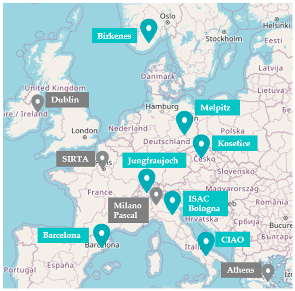
Figure 13. Observation network of the Aerosol, Clouds and Trace Gases Research Infrastructure (ACTRIS) considered in this work. The physical structure designed, built or installed to serve specific functions for research or monitoring purposes are shown in grey, while the ACTRIS national facilities, observational or exploration platform which has a contracts relationship with ACTRIS ERIC and which provides data and/or physical/remote access to its premises are shown in green. Source: https://ebas-data.nilu.no/, accessed on 1 July 2025.
Atmosphere 17 00677 g013
Figure 14. Spider diagrams for the 11 observation sites reporting the NR-PM1 percentage concentration calculated over the full analyzed period (May–October 2024).
Atmosphere 17 00677 g014
Table 1. Statistics of the mass concentrations (µg/m3) of the total NR-PM1 and of its components recorded by ToF-ACSM at CIAO from 13 May to 31 October 2024. Legend: m = mean value, md = median value, sd = standard deviation, max = maximum value, min = minimum value.
StatisticsOANO3SO42−NH4+ClTotal NR-PM1
m5.020.371.160.580.027.14
md4.430.300.890.500.026.43
sd3.120.271.100.410.064.24
max49.503.6511.704.175.9461.93
min0.03<LoD<LoD<LoD<LoD0.03
Table 2. NR-PM1 percentage concentration calculated over the full analysis period for CIAO and for ACTRIS OS where co-located ACSM measurements were available during the same timeframe. The year of analysis considered is shown next to the station name.
ACTRIS OSNH4+ClNO3OASO42−
Athens_DEM (2023)10.750.151.2374.7913.08
Barcellona (2020)10.110.591.9073.0714.33
Birkenes (2023)10.420.761.7381.875.22
CIAO (2024)8.100.315.1770.2116.22
Dublin (University college, 2022)12.811.812.7671.3811.24
ISAC Bologna (2023)11.970.213.3177.257.26
Jungfraujoch (2022)6.390.472.4486.713.99
Kosetice (2022)4.130.361.6285.868.03
Melpitz(2024)8.200.023.3780.048.37
Milano Pascal (2023)9.010.483.9876.3410.20
SIRTA (2024)9.420.843.2779.107.37
Disclaimer/Publisher’s Note: The statements, opinions and data contained in all publications are solely those of the individual author(s) and contributor(s) and not of MDPI and/or the editor(s). MDPI and/or the editor(s) disclaim responsibility for any injury to people or property resulting from any ideas, methods, instructions or products referred to in the content.