Robustness of PM_2.5 Source Allocation to Meteorological Variability—Evidence from 150 European Cities

Abstract

Ambient fine particulate matter (${\mathrm{PM}}_{2.5}$) poses a significant health risk in Europe, where many cities are exposed to levels exceeding WHO and EU guidelines. Reducing population exposure, therefore, calls for targeted and effective mitigation strategies. To support the implementation of optimal ${\mathrm{PM}}_{2.5}$ reduction policies, high-resolution air quality modeling is necessary. In this context, source allocation studies aim to link the pollution at a specific location to different emitters, typically expressing the contribution of each in terms of concentration differences. An alternative approach is the use of relative potentials, defined as the share of ${\mathrm{PM}}_{2.5}$ concentration reduced at a given receptor resulting from the reduction in the emissions from a given source. To calculate relative potentials, Source-Receptor Relationships (SRRs) can be used to mimic Chemical Transport Models, saving significant computation time when simulating emission reduction scenarios. However, while the relative potential indicator is increasingly used to guide source allocation analyses, its robustness with respect to meteorological variability has not been systematically evaluated. Given that meteorology can be a major driver of ${\mathrm{PM}}_{2.5}$ inter-annual variability, assessing this robustness is a prerequisite for the optimal use of SRRs in air quality planning. To address this gap, we use the SRR model SHERPA, based on the Chemical Transport Model EMEP, to evaluate the robustness of relative potentials of 150 European cities across four contrasting meteorological years (2015, 2017, 2019, and 2021). The contributions of four spatial reduction scales, six emission sectors and five emission precursors are analyzed. Our results show that relative potentials vary little with meteorology for most cities, with low inter-annual ranges for most spatial scales, precursors and sectors. These trends are consistent with EMEP simulations. They establish the robustness of the relative potential indicator and of SRR-based source allocations with respect to meteorological variability, supporting their use in guiding targeted air quality policies in Europe.

1. Introduction

Due to its high level of industrialization and development, Europe has many cities suffering from poor air quality, frequently exceeding both standards set by the European Union Ambient Air Quality Directive [1] and the guidelines established by the World Health Organization [2]. Notably, particulate matter (${\mathrm{PM}}_{2.5}$) is one of the pollutants most frequently implicated in such exceedances: many cities and regions in the continent do not meet the EU standards (daily mean concentration below 25 $\mathsf{\mu }$$\mathrm{g}·{\mathrm{m}}^{-3}$ more than 18 days a year, and yearly exposure below 10 $\mathsf{\mu }$$\mathrm{g}·{\mathrm{m}}^{-3}$), and only a few manage to keep concentrations below levels recommended by the WHO (daily mean concentration below 15 $\mathsf{\mu }$$\mathrm{g}·{\mathrm{m}}^{-3}$ more than 4 days a year, and yearly exposure below 5 $\mathsf{\mu }$$\mathrm{g}·{\mathrm{m}}^{-3}$). As a consequence, air pollution has led to 239,000 premature deaths in the EU-27 in 2022 through many diseases such as lung cancers, pulmonary diseases, cerebrovascular diseases and ischemic heart diseases [3].

Such numbers illustrate that air pollution remains the most critical environmental health hazard in Europe [4]. In recent years, different efforts have thus been suggested and then implemented at different spatial levels to mitigate air pollution [5,6,7]. Despite a noticeable enhancement in air quality over the years due to these actions [8], many European cities still experience ${\mathrm{PM}}_{2.5}$ levels exceeding both WHO and EU standards, particularly in high-density emission areas or cities with low wind conditions. Such levels can originate from direct ${\mathrm{PM}}_{2.5}$ (called primary particulate matter) emissions, as well as from secondary ${\mathrm{PM}}_{2.5}$ generated from precursors like non-methane volatile organic compounds (from sources like vehicles and industrial processes), nitrogen oxides, sulfur oxides and ammonia. This complex dependency on sources and atmospheric processes makes abating ${\mathrm{PM}}_{2.5}$ pollution a challenging issue. A fundamental concern is thus to determine the optimal scope of action, in terms of activity sector, in terms of emission precursor and in terms of spatial scale, in order to decrease the remaining air quality levels effectively.

To support the design of optimal air quality plans, a quantitative assessment of the different sources contributing to air pollution is needed. In the European Union, this is a legal obligation for countries and regions whenever exceedances occur. This research field, known as source allocation, has been the subject of many studies in recent years. Most of them rely on the use of Chemical Transport Models (CTMs) that simulate the behavior of atmospheric pollutants [9,10,11,12]. They are generally associated with bottom-up inventories that include direct ${\mathrm{PM}}_{2.5}$ emissions, as well as emissions of precursors of secondary particulate matter [13,14]. Because CTMs simulate transport, diffusion, and chemical transformation processes, they enable assessing the impact of emissions reductions over various spatial domains, such as cities, regions, countries, or country groups, on air quality levels. By performing multiple simulations, they allow characterizing the statistical distribution of air composition resulting from the implementation of different emission reduction scenarios. This enables the attribution of the different contributors to the air quality of a given point in space, generally expressed in terms of concentration differences in source allocation studies [15,16]. However, CTMs require intensive computational resources, which limits their use to a detailed analysis for one city or region at a time only. As a consequence, quantifying high-resolution source allocations at the scale of Europe is prohibitive. To overcome this constraint, the “Screening for High Emission Reduction Potentials for Air quality” model (SHERPA) has been developed by the Joint Research Centre [17]. This model is a screening tool, constructed from a set of air quality simulations from a given CTM, achieving similar results but more rapidly.

Since source allocation results inherently depend on the meteorological conditions used to train the model, the robustness of SHERPA-based source allocations with respect to inter-annual meteorological variability must be assessed. While previous studies have validated SHERPA against its underlying CTM and applied it to support air quality planning, this sensitivity to meteorological variability has not been systematically investigated. This represents an important knowledge gap, as meteorological variability strongly influences ${\mathrm{PM}}_{2.5}$ concentrations and could potentially affect the identification of priority sectors, precursors and spatial scales for emission reduction. The objective of this study is, therefore, to quantify the influence of meteorological variability on the sensitivity of ${\mathrm{PM}}_{2.5}$ concentrations to emission reductions. To this end, SHERPA is used to attribute the origins of air pollution for a set of 150 European cities distributed throughout Europe and for four meteorological years: 2015, 2017, 2019 and 2021 (the selection of these years balances data coherence, availability, and avoids COVID-19 impacts in 2020 for reliable meteorological analysis). For each city, the spatial, sectoral and precursor contributions to the urban ${\mathrm{PM}}_{2.5}$ concentrations are quantified and compared for these meteorological years. To allow fair comparisons between regions with different concentration levels and an assessment of the contributors with the highest mitigation leverage in the context of air quality control, absolute concentration differences are not sufficient. For this reason, we employ the concept of “relative potentials” as an alternative statistical indicator to express source allocations. It is defined as the proportion of ${\mathrm{PM}}_{2.5}$ concentration decrease at a receptor point due to the abatement of emissions from a specific precursor-sector-area source ensemble, capturing the sensitivity of a region to emission reductions. The novelty of the present work is, therefore, to provide the first large-scale assessment of the robustness of both the SHERPA source-allocation methodology and the relative potential indicator with respect to meteorological variability across Europe. This article is structured as follows: Section 2 describes the SHERPA tool and its underlying CTM and details the methodology of this study. Section 3 analyses the source allocations for 150 urban areas and their variabilities with respect to the meteorological input, with a focus on spatial scales, sectors and precursors. Section 4 assesses the robustness of the results with respect to meteorological variability by comparing the SHERPA results to standard air quality simulations. Finally, the main uncertainties associated with the source allocation results are presented in Section 5. City names are written in the language of their country or region using the Latin alphabet.

2. Materials and Methods

2.1. City Targets

To analyze a wide range of source allocations, our study focuses on 150 major European cities (all located in the EU-27, the United Kingdom, Switzerland and Norway), already analyzed in the ${\mathrm{PM}}_{2.5}$ atlas [18], and that account for many registered exceedances of EU air quality standards. The source allocation is performed at four distinct spatial scales (where emission reductions apply): Europe, the country, the “greater city” region and the “city core” region. Core cities correspond to city centers with a density greater than 1500 $\mathrm{hab}·{\mathrm{km}}^{-2}$ and a total population greater than 50,000 inhabitants. The term “greater city” corresponds to the concept of “functional urban area” and consists of the core city as well as its extended commuting zone, defined as the surrounding zones where at least 15% of employed residents work in the city within the corresponding country, i.e., without taking cross-border commuting into account. Such quantitative definitions, described by OECD [19], are used here to harmonize the city dataset.

2.2. EMEP Simulations and Meteorological Inputs

The EMEP MSC-W (called EMEP henceforth) model [20] is a CTM that was established by the European Monitoring and Evaluation Programme (EMEP) for Transboundary Long-Range Transported Air Pollutants. The model focuses on Europe, with a domain stretching from −15.05° to 36.95° in longitude and 30.05° to 71.45° in latitude, with a horizontal resolution of 0.1° × 0.05° (i.e., ∼11 × 4 ${\mathrm{km}}^2$ at European mid-latitudes). Twenty vertical levels are used, with the first level around 45 m. Meteorological input data is provided with a daily resolution, while a 3-h timestep is used for outputs. The model simulates particulate matter, photo oxidants, inorganic and organic gases and pollutants, as well as wet and dry deposition. Status reports for EMEP, including comparisons with in situ measurements, are available at https://www.emep.int/publ/common_publications.html (accessed on 16 June 2026). For the purpose of this study, European air quality simulations using version 4.5 of the model are driven by meteorological fields from the European Centre for Medium-Range Weather Forecasting (ECMWF-IFS). The simulations are conducted for the years 2015, 2017, 2019, and 2021, using corresponding initial and boundary conditions. These are prescribed within the EMEP framework rather than dynamically provided by an external global chemistry model. They include Saharan dust, sea salt, and ozone fields, while sulfate, nitrate, and ammonium are represented by fixed background concentrations. Initial ozone concentrations are based on observations. Anthropogenic emissions underlying the model simulations are based on version 6.1 of the Copernicus Atmosphere Monitoring Service (CAMS) emissions (including condensables) per country-pollutant-sector for 2019, based on Denier van der Gon et al. [21]. This regional anthropogenic emission inventory covers emissions for UNECE-Europe for the main air pollutants and greenhouse gases [22]. The use of these fixed annual emissions for all four simulations allows focusing on the influence of meteorological variability, but are not meant to represent real year-to-year changes in anthropogenic emissions. The only combined effect of changing emissions and meteorology concerns emissions of the residential sector (through domestic combustion for heating), whose distribution throughout the year is changed through the use of pre-calculated degree-day factors for each day of the year, while conserving the total annual emission budget. This effect is, however, negligible on the variability of annual emissions of all species. For other air quality parameters, background and initial conditions are set within the model using functions based on observations [9,23]. Secondary aerosol formation accounts for complex chemical and physical processes, such as sulfate aerosol formation from sulfur dioxide, nitrate aerosol formation from nitrogen oxides, or organic aerosol formation from volatile organic compounds. More detailed information on the boundary conditions, meteorological drivers, land cover, model physics, and chemistry is provided in de Meij et al. [24], Simpson et al. [20] and in the EMEP Status Report 2019 [25]. The accuracy of the EMEP model has been evaluated through comparisons with observational data of ${\mathrm{PM}}_{2.5}$, ${\mathrm{PM}}_{10}$, ${\mathrm{NO}}_2$, and ${\mathrm{O}}_3$, as reported in Thunis et al. [26].

These four simulations, called “Base Case”, differ in terms of weather conditions. The EMEP Status Reports of 2017, 2019, 2021 and 2023 (corresponding to the meteorological years 2015, 2017, 2019 and 2021, respectively) indicate distinct annual anomalies in temperature and precipitation across Europe, including regional extreme events that are not reproduced from one year to another. These analyses suggest that the selected years encompass a broad range of meteorological conditions relevant for the study of ${\mathrm{PM}}_{2.5}$. For instance, total rainfall was higher in 2017 and 2021 than in 2015 and 2019 for Baltic States and neighboring countries, while it is lower for countries in southern Europe. Annual temperatures are also lower in central and eastern Europe in 2021 compared to other years. Finally, ${\mathrm{PM}}_{2.5}$ concentrations calculated by EMEP have a higher annual average in Poland in 2021. That year, annual ${\mathrm{PM}}_{2.5}$ concentrations are also higher in southern Italy and, to a lesser extent, in the Balkan Peninsula, which is likely related to enhanced Saharan dust intrusions. These intrusions, known for their strong inter-annual variability in this region [20], were 60 to 120% higher in 2021 than in 2015–2017–2019 average. In addition to these Base Case simulations, six EMEP simulations are performed for each of the four meteorological years. These simulations comprise five scenarios reducing one emission precursor at a time (reducing nitrogen oxides, volatile organic compounds, ammonia, primary ${\mathrm{PM}}_{2.5}$ and sulfur oxides) by 50% and one scenario reducing emissions of all precursors at the same time. These six additional simulations are called “−50% scenarios”.

2.3. Methodology and Reduction Metrics

EMEP simulations can be used to calculate the impact of an emission scenario policy by comparing simulated ${\mathrm{PM}}_{2.5}$ concentrations in the Base Case with those in the −50% scenarios. Formally, the concentration change $\Delta C$ at a receptor point is the annual concentration change between the Base Case concentration $C_{\mathrm{BC}}$ and the scenario concentration $C_{\mathrm{scenario}}$. When anthropogenic emissions are reduced with an abatement level $\alpha$ for a given precursor, this difference is expressed as follows:

$$\Delta C=C_{\mathrm{BC}}-C_{\mathrm{scenario}}\left(\alpha \right)$$

(1)

While this metric is simple and intuitive, it is insufficient for this study because it is expressed in absolute terms. Indeed, if large inter-annual variations in background ${\mathrm{PM}}_{2.5}$ concentrations occur due to meteorology or long-term emission trends, a given absolute concentration difference may be negligible in a highly polluted year but critical in a cleaner year. Thus, comparing absolute concentration changes across years does not provide meaningful information on the avoidance of air-quality exceedances. As such, concentration differences do not allow for comparing cities that are characterized by very different absolute concentration levels and are insufficient to inform emission-reduction policies aimed at compliance with limit values. Here, we use the “relative potential” $RP$, which is a more robust statistical indicator for understanding the effect of emission reductions on ${\mathrm{PM}}_{2.5}$ concentrations. It is defined from the former quantities as follows [27]:

$$RP={\displaystyle \frac{C_{\mathrm{BC}}-C_{\mathrm{scenario}}\left(\alpha \right)}{\alpha C_{\mathrm{BC}}}}$$

(2)

The two metrics above differ in their sensitivity to inter-annual variations. Concentration differences can vary significantly from year to year due to changes in meteorology and emissions, while relative potentials can potentially remain stable due to concomitant changes in background concentrations. Indeed, when background concentrations vary strongly while concentration differences remain similar, the relative potential changes accordingly. Conversely, when background concentrations and concentration differences vary proportionally across years, the relative potential remains stable. In the Supplementary Materials, the inter-annual ranges throughout the four studied years (defined as the difference between the maximum and minimum annual values) of concentration differences and relative potentials are mapped (Figure S1), showing no proportionality between the two metrics. Seven examples of cities also illustrate the differences between the variations in the two indicators (Figure S2). The relative potential thus captures the sensitivity of a region to emission reductions and provides a more consistent indication of its response. When assuming linearity between emission changes and concentration changes, the relative potential is independent of the abatement level, i.e., a constant only representing the sensitivity of a receptor to emission reductions from a source for a particular sector or precursor. Thunis et al. [28] have shown that for annual means, this linear assumption remains valid (no interaction terms) for abatement levels up to $\alpha$ = 50%, hence the choice of this value for the used emission reduction scenarios. Below this value, the metric is robust, allowing for the specific sensitivity of each region to pollutant emissions to be taken into account. Above this value, however, non-linear conditions are reached, and this approach can no longer be used to assess the consequences of abatement strategies. Note that this threshold is only valid for ${\mathrm{PM}}_{2.5}$ and for yearly average concentrations. Its main advantage is that it makes the relative potential independent of the level of emissions reduction, making it a more robust tool for comparing results between different regions.

2.4. The SHERPA Modeling Tool

While EMEP can, in principle, be used to estimate the relative potential of cities for different sources, doing so would require numerous simulations covering various combinations of precursors, sectors and spatial scales. To overcome this limit, the “Screening for High Emission Reduction Potentials for Air quality” (SHERPA) was developed during the last ten years. It is a decision-support tool that enables the evaluation of potential air quality improvements resulting from the implementation of emission reduction measures in specific sectors and geographic areas [17]. It is based on Source-Receptor Relationships (SRRs). These SRRs are a simplified version of a CTM, used to simulate the contribution of precursor emissions within a domain of application to air quality levels. More specifically, they are used to estimate the effect of changes in precursor emissions applied over a given area on concentrations of ${\mathrm{PM}}_{2.5}$ at a given receptor point. This is called a source allocation. In general, an SRR model is a system of algebraic relationships linking gridded precursor emissions and concentrations by a series of unknown coefficients that are identified based on a limited series of full CTM simulations. These unknown coefficients represent the interactions between source cells and receptor cells. In SHERPA, such interactions vary from one cell to the other, and they are described by a bell-shaped function, which is characterized by two parameters representing the extent and the intensity of the interaction. This assumes that the impact of emissions of a source cell on the concentration at a receptor cell decreases with the distance between the two corresponding pixels. A more complete description of SHERPA is provided by Pisoni et al. [29]. One of the advantages of this grid-to-grid SRR is its potential to analyze a wide variety of scenarios: SHERPA can be used to quantify the effect of emission reductions applied over any set of grid cells on any given location. In this model, cities, regions, and countries are approximated by clusters of contiguous cells within a given polygon representing their spatial extent. Within those clusters, emission reductions are applied to model air quality policies. By selecting a specific location, the sectoral or precursor contributions from a chosen area can be explicitly quantified, reflecting the potential air pollution impacts of reducing emissions from a particular sector or spatial scale. In its current configuration, SHERPA is trained with the EMEP simulations for the four different meteorological years described in Section 2.2, covering the whole of Europe with a horizontal resolution of ∼7 km. City clusters are derived from the OECD (Urban Audit) polygons and mapped onto the SHERPA grid by retaining the model cells with at least 75% of their area within the corresponding city boundaries. Each city is represented by a receptor point, defined as the cell with the highest concentration within the resulting city cluster, following the standard SHERPA methodology adopted in previous studies to ensure comparability of results. The use of these different meteorological years provides a more robust understanding of how climate variability affects the source apportionment estimates. Because of its simplifying assumptions and spatial resolution, SHERPA is limited to calculating mean annual ${\mathrm{PM}}_{2.5}$ concentration levels for cities of sufficiently large size (i.e., a minimum area of 300 ${\mathrm{km}}^2$). As such, it is designed to evaluate the long-term effectiveness of emission reduction strategies, but it is not intended to capture short-term, meteorologically-driven pollution events.

Here, we use SHERPA to approximate the relative potential of cities for different sources, defined here as a group of grid cells for which one or more precursors and one or more sectors are considered. The relative potential of a given receptor is always calculated with respect to a given precursor–sector–area source ensemble. From a policy point of view, sources with high relative potentials are the ones to be addressed first to achieve the largest improvements. In this work, the SRRs are calculated for emission reductions performed with $\alpha$ = 50%. As expected above, non-linear effects on the estimation of relative potentials remain limited, as shown in previous SHERPA studies [30]. The aim of this work is to analyze how the main contributors to urban pollution in terms of sectors, geographical areas and precursors vary with the meteorological conditions. Four scales are analyzed for each city in the dataset:

• the core city,
• the commuting zone (rest of the greater city),
• the rest of the country and
• the rest of Europe.

When all these spatial reduction scales are considered together (i.e., a Europe-wide emission reduction), the term “total relative potential” is used. The precursors that are considered are as follows:

• primary particulate matter (${\mathrm{PPM}}_{2.5}$),
• non-methane volatile organic compounds (NMVOCs),
• nitrogen oxides (${\mathrm{NO}}_{\mathrm{x}}$),
• sulfur oxides (${\mathrm{SO}}_{\mathrm{x}}$) and
• ammonia (${\mathrm{NH}}_3$).

Finally, the sectors that are considered are those defined as in the ${\mathrm{PM}}_{2.5}$ atlas. The correspondence with the Gridded Nomenclature For Reporting (GNFR), which is an aggregated version of the Nomenclature For Reporting to the EU [31], is the following:

• industry (GNFR A + GNFR B),
• residential (GNFR C),
• agriculture (GNFR K + GNFR L),
• transport (GNFR F + GNFR I),
• shipping (GNFR G) and
• others (GNFR D + GNFR E + GNFR H + GNFR J).

For all precursor-sector-area emission reduction scenarios, the relative potentials of each of the 150 European cities are assessed at the location of maximum concentration within the city core, which is assumed to represent the most challenging pollution exposure.

3. Results

3.1. Source Allocation Results by Spatial Scale

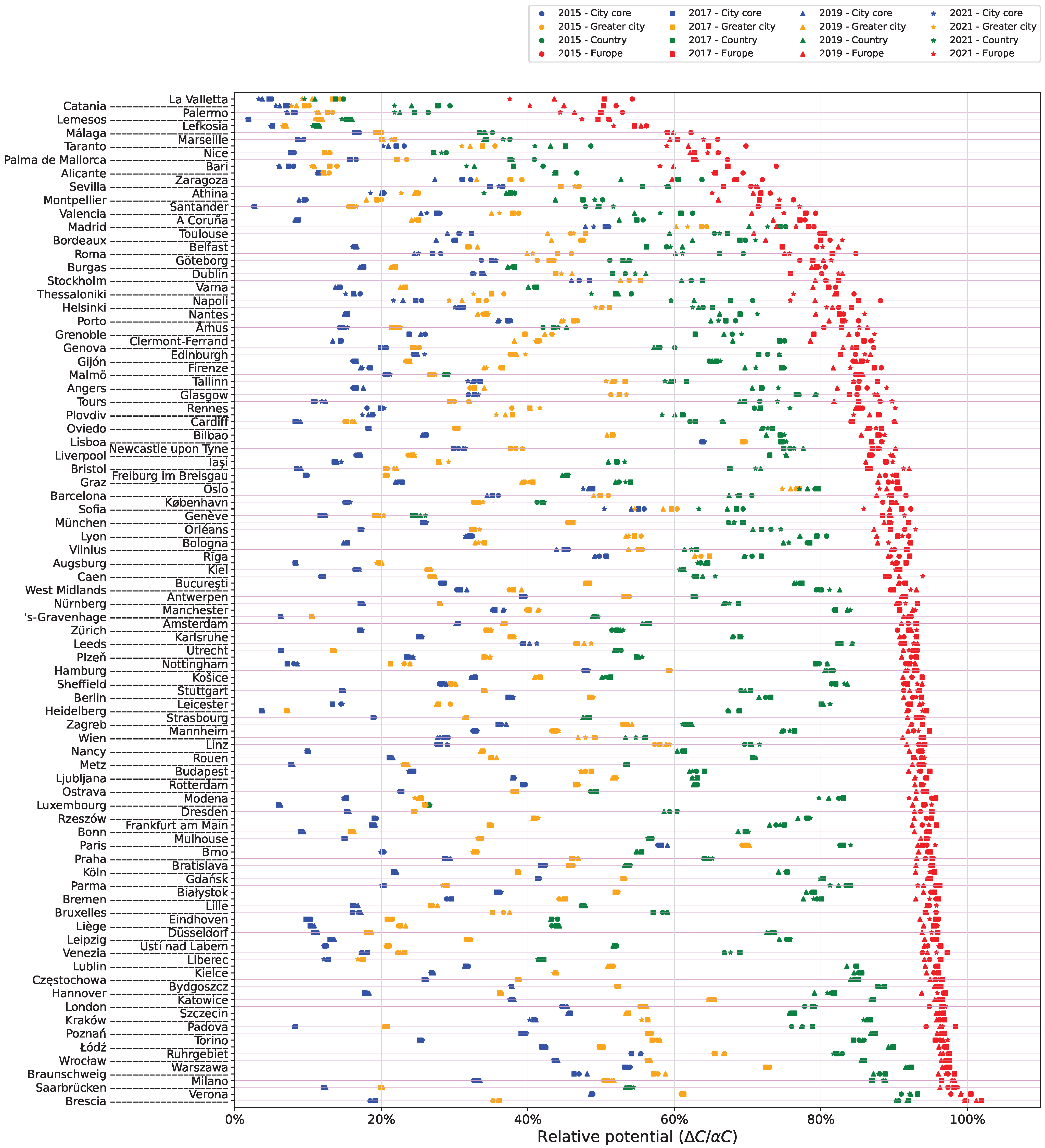
We analyze SHERPA outputs across the four distinct years to evaluate the meteorological variability of source allocations. For each city, when progressively summing spatially relative potentials, the contributions of the city core, the greater city, the corresponding country and the entire domain of application (Europe) are obtained. Figure 1 shows, for all cities, the progressive relative potentials when cumulated by spatial scales of reduction. Cities are ranked on the basis of the mean total relative potential. Results for individual reduction scales are presented for all cities in the Supplementary Materials (Figures S3–S6). On average, 2015 and 2019 have total relative potentials higher than for the other years, with maxima in 104 of the 150 cities. Conversely, 2017 and 2021 have the minimum total relative potentials for 89 of the 150 cities. The orders of magnitude reached by the averaged relative potentials are similar to those obtained in previous SHERPA validation studies [32]. Overall, coastal cities in the southern part of the domain have the lowest total relative potential: for all four meteorological years, 14 out of the 15 cities with the lowest total relative potential are located in Malta, Cyprus, Greece, southern Spain, southern Italy, and southern France. In particular, Lemesos and Lefkosia (Cyprus), Catania and Palermo (Italy) and La Valletta (Malta) have the five lowest total relative potentials for all meteorological years, with total relative potentials never exceeding 60%. However, while meteorology has little effect on the order of these five cities, it has an effect on the amplitude of the relative potential, with 2015 generally having the highest relative potential values and 2021 the lowest. Here, these low values can be interpreted as mostly due to non-anthropogenic ${\mathrm{PM}}_{2.5}$, in the majority of dust, originating from beyond the domain boundaries, particularly from the Sahara in the case of Malta and southern Italy. As dust transport can vary largely with years, it is likely to be the main driver of the observed variability for southern cities. Extending this interpretation, a year with a prolonged Saharan dust intrusion, whose magnitude and spatial extent differ substantially from those considered in the four years under study, would increase this variability even further, leading to relative potential deviations for mid-latitude European cities compared to the behavior observed here. Dust intrusion could, as a consequence, limit the feasibility of remaining below the guidelines in terms of annual concentrations even with the implementation of ambitious emission reduction policies. Note that this effect is limited to other cities near other domain boundaries (Atlantic, European sub-Arctic and Russia, approximately), due to limited biogenic emissions and fine particle transport there. Conversely, the regions with the highest relative potentials are those with the highest absolute pollution levels and far from the boundaries of the domain, such as cities in the Po Valley and Poland. In these regions, relative potentials vary little from one meteorological year to another. The combination of low inter-annual meteorological variability and high relative potentials makes these regions those where emission reduction policies are both the most reliable, yielding consistent responses across years, and the most effective, leading to substantial air quality improvements.

When analyzed at each individual reduction scale (i.e., without cumulating lower spatial scales), cities have relative potentials similar to those calculated in previous SHERPA validation studies: on average, city cores have an average relative potential similar to that of the rest of the country and that of the rest of the domain (about 25%), while the relative potential associated with the commuting zone only is lower (about 13%), generally due to a much smaller size, population or density of the commuting zone in comparison to the city core. Some cities like Bilbao (Spain), Clermont-Ferrand (France), Katowice (Poland), Oslo (Norway), Linz (Austria), and Torino (Italy) have a higher contribution to the commuting zone, often due to their larger size or population. When considering the entire functional urban area (city core and commuting zone), larger metropolitan areas tend to have higher relative potentials. For each meteorological year, the seven megacities of the dataset (Paris, France, London, United Kingdom, Madrid and Barcelona, Spain, Milano, Italy, the Ruhrgebiet area and Berlin, Germany, with more than 5 million inhabitants each) have relative potentials for the functional urban area above the 75th percentile (i.e., the first 37 cities), except Berlin which ranks 38th and 40th in 2015 and 2017. At the country scale, medium-sized cities located near other cities in the same country, but relatively isolated from the rest of the continent, have emissions influencing each other, leading to significant relative potentials associated with country emissions, particularly in the Po Valley (Bologna, Brescia, Modena, Padova, Parma, Venezia) and England/Wales (Bristol, Cardiff, Leicester, Liverpool, Nottingham, Sheffield). For these cities, a synchronized and coordinated emission reduction policy is, therefore, optimal to effectively limit exceedances of air quality standards.

Cities for which the rest of Europe contributes the most to the total highest relative potential are those close to international borders or in small countries. Luxembourg City (Luxembourg), Genève (Switzerland), Malmö (Sweden), Liberec (Czechia), Eindhoven (Netherlands) and Liège (Belgium) are cities for which this contribution is the highest for the four meteorological years, with a value always higher than 50%. Finally, it must be noted that the two Italian cities of Brescia and Verona reach relative potential values for Europe that are slightly higher than 100% for some years. This value is physically impossible (the maximum value being 100%, corresponding to an air totally clean of ${\mathrm{PM}}_{2.5}$) and denotes the presence of non-linearities that are not accounted for in SHERPA, which are frequent in the Po Valley where inorganic aerosol formation is significantly driven by ${\mathrm{NH}}_3$ and ${\mathrm{NO}}_{\mathrm{x}}$ chemistry [33]. However, since the effect of these non-linearities is minor, as explained in Section 2.4, it is likely that a more accurate estimate of the relative potential of these two cities would lead to values close to 100% like the majority of cities in the Po Valley (Milano, Torino, Padova, Venezia, Modena).

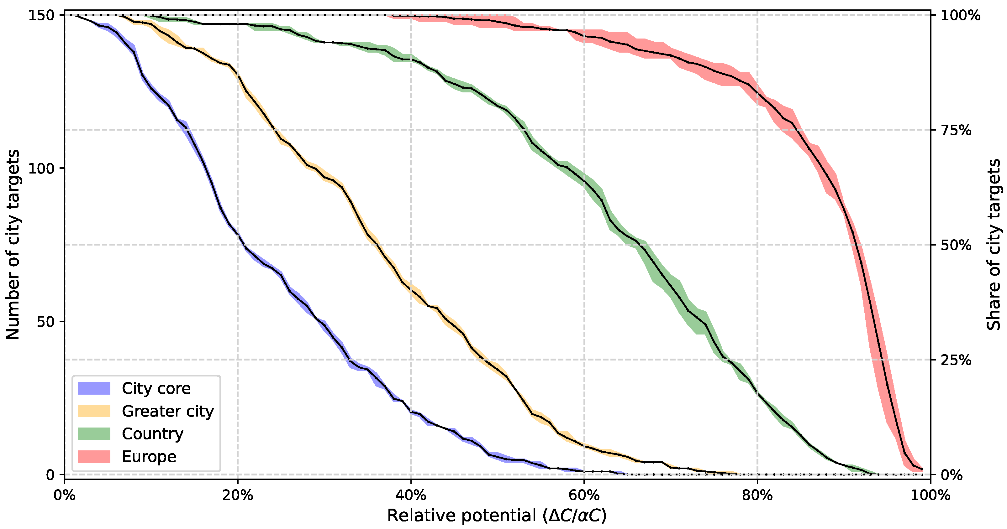
For policymaking purposes, such results can be analyzed statistically. By counting the number of cities in the set that exceed a given relative potential threshold, we can determine the optimal level of action. Conversely, by setting a given reduction scale, we can identify the number of cities whose exposure will be reduced by a given percentage. This is illustrated in Figure 2. Although the number of cities reaching a given level of reduction changes little from one meteorological year to the other, this variability generally increases with the spatial scale chosen. The lower contribution of commuting zones alone to the total relative potential, previously identified, is also highlighted here. Here, the relative potential reaches 50% or more for a country-wide reduction for 120 to 121 of the cities, and this number rises to 146 to 150 for a European reduction. Conversely, there are only 5 to 7 cities where the relative potential exceeds 50% when emission reductions are applied on the city core alone: Lisboa (Portugal), Paris (France), the Ruhrgebiet area (Germany), Sofia (Bulgaria), Warszawa (Poland), Rīga (Latvia), one out of four times and Madrid (Spain) two out of four times. Since the relative potential levels remain consistent across different meteorological years, the conclusions drawn from this analysis are not strongly affected by meteorology. This illustrates the dominance of large, industrialized urban areas, which concentrate human activity within their region, and therefore, account for the majority of the pollution they experience. A comparison with the CAMS Policy Support Tool (https://policy.atmosphere.copernicus.eu/daily/country-impact/, accessed on 22 June 2026) generally supports these results, with the city core being responsible for the absolute majority of ${\mathrm{PM}}_{2.5}$ in Madrid, Sofia, and Lisbon, and a relative majority in Rīga and Warsaw. However, for Paris and the Ruhrgebiet area, it indicates a smaller core contribution, which might suggest local-specific factors or methodological differences in source apportionment.

3.2. Variability of Relative Potentials for Spatial Scales

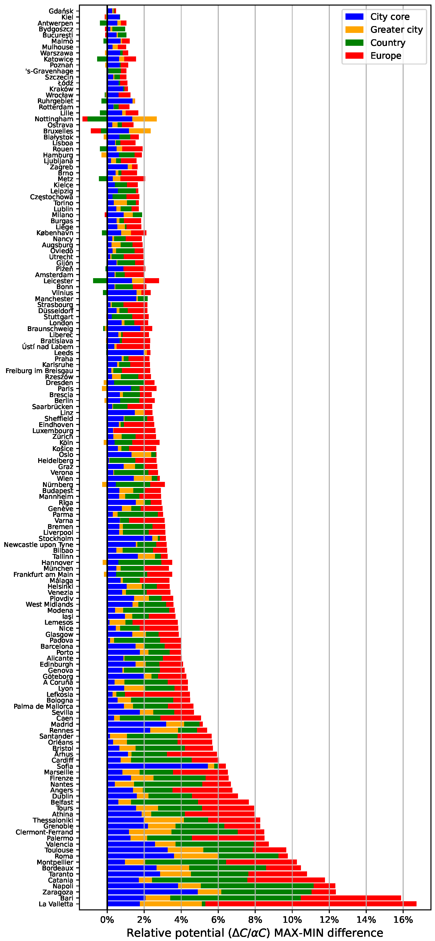
Although Figure 1 and Figure 2 show the low variability of the relative potentials at all reduction scales, they do not make it possible to determine which spatial scale of emission reduction contributes most to this variability, or whether spatial scales tend to stabilize relative potentials in certain cities. For each city, we thus calculate the variability of the relative potential for the different cumulated spatial scales of emission reduction. Figure 3 shows this variability, expressed in terms of inter-annual range. To provide a policy point of view, the contribution of each spatial scale of reduction is calculated to illustrate the variability of impacts related to measures that would be taken at different administrative levels. Here, moving from a spatial scale to a higher one generally comes with an increased variability of the relative potential, hence the rare and low negative values in Figure 3. The main observation is the low variability reached by the total relative potential, with 9 out of 10 cities having an inter-annual range never exceeding 8%. We also observe that the highest variabilities are found for cities that have a low average relative potential for the European scale. They are mostly located in southern Europe, such as La Valletta, Malta (16.7%), Bari, Italy (15.9%), Zaragoza, Spain (12.4%), Napoli, Italy (12.3%), and Catania, Italy (11.7%). These cities all have a Europe-scale relative potential that is lower than the 10th percentile of the city distribution, except for Naples, which ranks 31st out of 150. Conversely, the lowest variabilities are mostly found for cities bordering the North and Baltic Seas. Overall, it is observed that for all spatial scales of emission reductions, the relative potentials of cities calculated with SHERPA vary very little with meteorology. Except for La Valletta, this variability is never higher than a quarter of the mean total relative potential. The commuting zone contributes the least to the variability in relative potential, with the other three spatial scales making similar contributions on average. Moving from a reduction scale to a larger scale only rarely reduces the variability of the relative potential obtained. These results are important in two respects. From a modeling perspective, they demonstrate the robustness of the source allocation results to meteorological variability and suggest that future SRR models such as SHERPA might function on the basis of a single meteorological year of simulations for most cities on the continent. From a policy perspective, it increases the confidence that the priority and actions planned for a given year regarding yearly exposures will remain relevant and efficient regardless of the meteorological conditions.

3.3. Source Allocation Results by Sector and Precursor

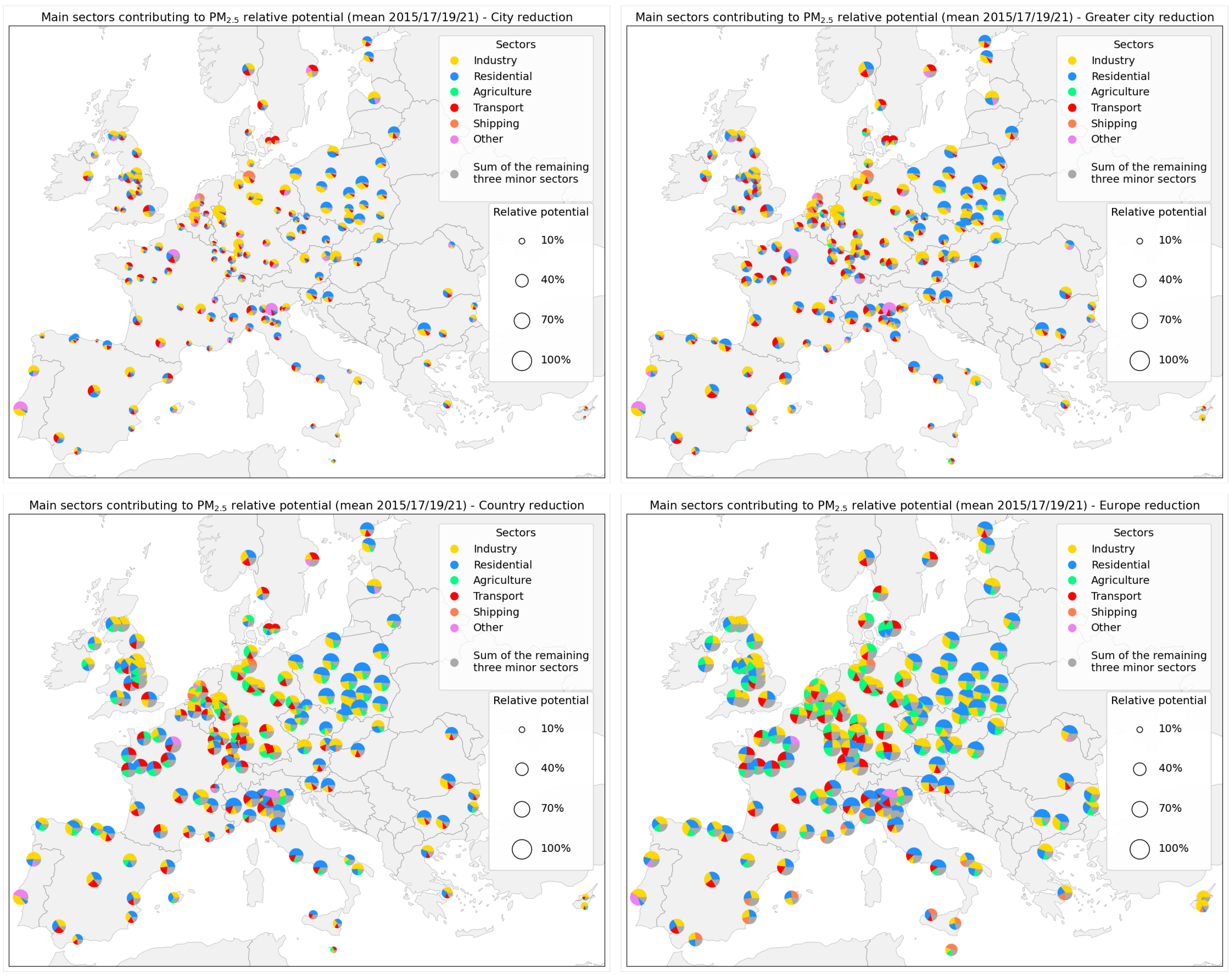
The previous results showed a low variability in the relative potential of each city calculated for all four spatial scales of emission reduction. This low variability is also found for activity sectors. Here, 25 cities have a change in dominant sector between two (and sometimes three) meteorological years, with most of them being located in France and Germany. For 17 of them, only one scale of reduction is concerned. These changes in the dominant sector generally happen between sectors that have similar shares. Figure 4 breaks down the mean relative potential (i.e., averaged for the four years under study) by activity sectors for the four reduction scales. For reductions performed at the scale of city cores and greater cities, the residential sector generally has the highest relative potential, followed by the industry sector, except for German cities, where the industry sector frequently has a higher relative potential. The share of the transport sector in the total relative potential varies significantly from one city to another, without a clear parameter characterizing high shares for it. The agricultural sector accounts for a minority share of the total relative potential for the city core or the greater city, but gains significant importance at the scale of emissions performed at the scale of the country, especially in Western and central European cities. It is, however, never the dominant sector, except for the relative potential of Aarhus (Denmark) for country or European emission reductions. Finally, the relative potentials of southern cities for shipping emissions are generally high, with even a dominance of this sector for Palma de Mallorca (Spain), Málaga (Spain), La Valletta (Malta), Catania (Italy), and Palermo (Italy). The “Other” category, which groups aviation, waste, solvents and fugitives, dominates the relative potential of Paris (France) and Verona (Italy) for all scales of reduction. It is also the case of Lisboa for the first three spatial scales of reduction.

Generally speaking, the sensitivity of source allocations expressed in terms of sectors is low. Relative meteorological variabilities (here defined as the difference between the maximum and minimum relative potentials achieved over the four meteorological years, divided by the corresponding average) are lower than 25% in 90% of the cases. The highest values are found for agriculture, especially in southern European cities and in Ireland. Large meteorological variabilities for the “Other” sector only concern a very small number of cities. Note that these variabilities are calculated on a relative basis to identify the most sensitive sectors and do not necessarily reflect the variability of the total relative potential. To do so, the variability must be calculated in absolute terms. In this case, industry contributes on average to 26% of the variability of the relative potential for Europe, followed by agriculture (25%), the residential sector (19%) and transport (16%). At lower spatial scales, however, the contribution of agriculture diminishes while industry remains the main contributor to variability. For a given sector except agriculture, its share in the meteorological variability of the total relative potential increases with its contribution to the mean relative potential over the city dataset, with a mean ratio of the two shares usually between 0.5 and 2.7. A relatively high correlation is found ($R^2>0.5$) between the two ratios. Agriculture is the only sector for which no significant correlation is found between the two shares. In the Supplementary Materials (Figure S10), the comparison of these two ratios is shown for the six sectors. To illustrate this, port cities in southern Europe, where the shipping sector has a major share of the relative potential, are also subject to a high meteorological variability. For example, La Valletta’s 4-year average total relative potential is 46.4%, of which 20.5% comes from the shipping sector, 7.5% from industry, 6.9% from agriculture and 5.8% from transport. The total meteorological variability of this relative potential is 16.7%, and the variability in the shipping sector alone is 6.3%, ahead of agriculture (5.1%), industry (2.1%) and transport (2.0%). In this case, the shipping sector, which is the largest contributor to the total relative potential, is also the largest contributor to the meteorological variability, while having a corresponding relative variability lower than other sectors. From a policy point of view, this result suggests that the implementation of a policy aimed at reducing emissions from the sector that contributes most to ${\mathrm{PM}}_{2.5}$ levels in a city (unless it is the agriculture sector) will generally be accompanied by a reduction in ${\mathrm{high-PM}}_{2.5}$ concentration periods.

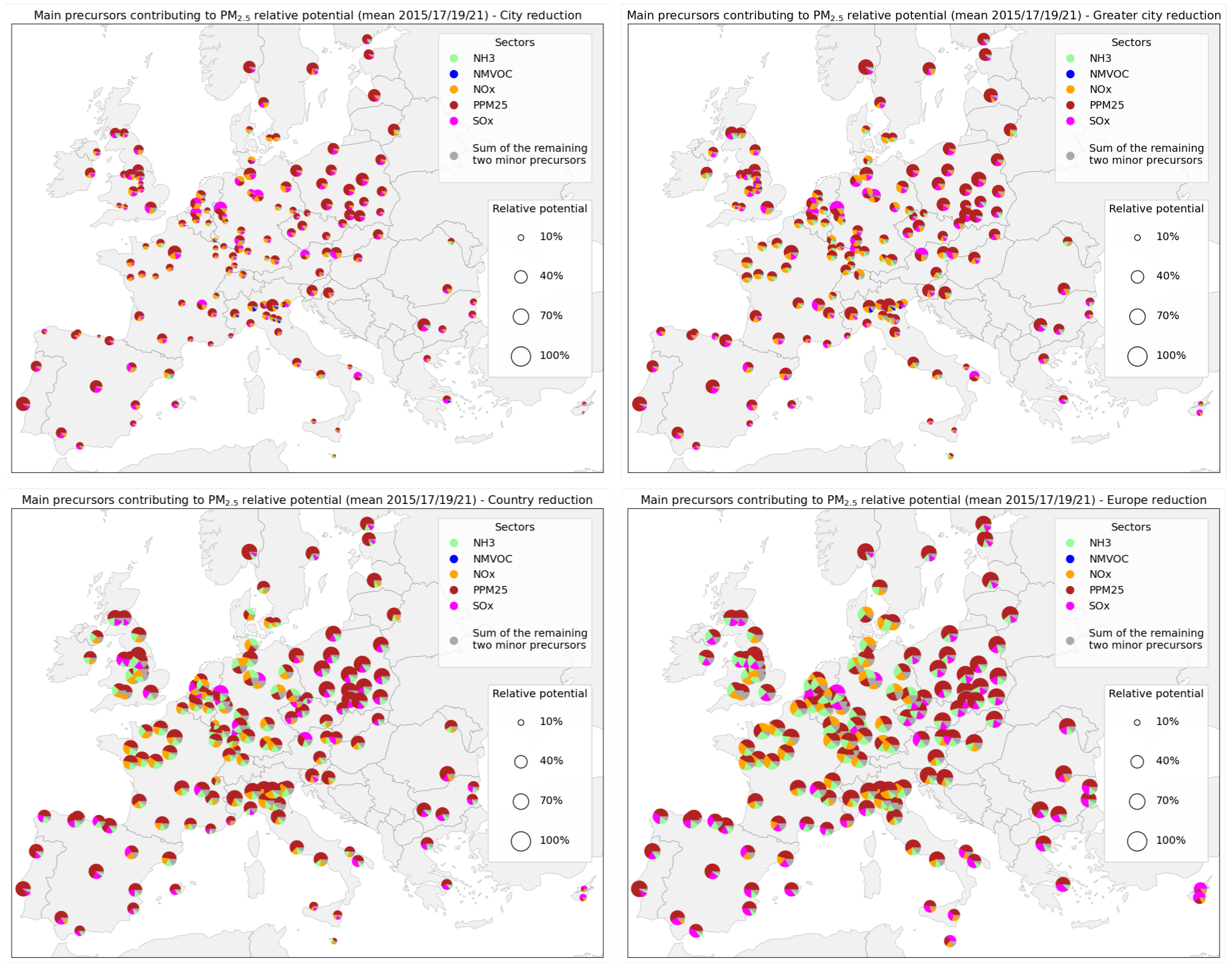
Source allocation can also be carried out at the precursor level, making it possible to support reduction policies by influencing the technological aspect of emission processes. Figure 5 breaks down the mean relative potential by precursor for the four reduction scales, showing a clear dominance of primary particulate matter (${\mathrm{PPM}}_{2.5}$) in the relative potential for most cities in the continent, generally followed by ${\mathrm{SO}}_{\mathrm{x}}$ at the city core level, except for most cities in France and northern Italy where the second precursor is generally ${\mathrm{NO}}_{\mathrm{x}}$. Ammonia emissions gain importance from the scale of reduction corresponding to national reductions, due to the incorporation of agricultural emissions, which are dominated by this precursor. At the European scale, only Lefkosia and Lemesos (Cyprus) and La Valletta (Malta) have relative potentials not dominated by primary particulate matter but by ${\mathrm{SO}}_{\mathrm{x}}$. Non-methane volatile organic compounds are associated with low relative potentials for all cities of the continent and at all scales of reduction, except for cities in the Po Valley, where they can be noticeable. While primary PM accounts for around half of the relative potential for Europe, it contributes to only a quarter of the corresponding mean meteorological variability. ${\mathrm{NO}}_{\mathrm{x}}$ and ammonia account for around a quarter of the total meteorological variability each, despite contributing much less to the total relative potential. ${\mathrm{SO}}_{\mathrm{x}}$ accounts for around 16% of the total meteorological variability, but plays a more significant role in coastal cities, with Lemesos (Cyprus), Burgas (Bulgaria), Málaga (Spain), and Lisboa (Portugal) having shares of more than 25% of the total variability. The only other examples of high contributions for ${\mathrm{SO}}_{\mathrm{x}}$ include München (Germany), and Leeds (United Kingdom). Finally, non-methane volatile organic compounds are the precursors that contribute the least to the meteorological variability for Europe. At the city core scale, however, they can account for a significant share of the variability in some cities in Italy, the Netherlands and eastern France.

4. Comparison with CTM Outputs

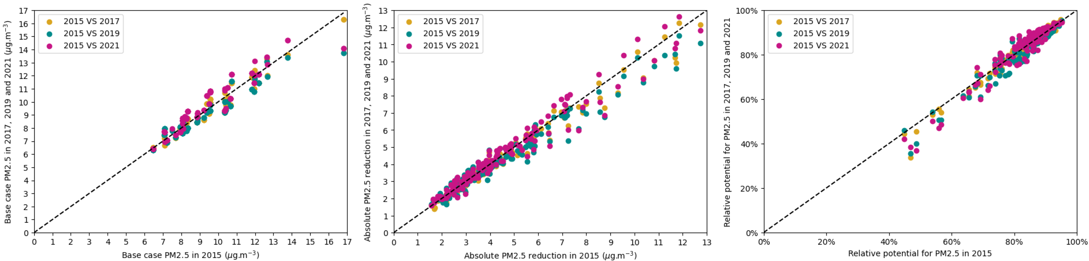
Studies that were already conducted on the validation of SHERPA showed an agreement of the outputs calculated between SHERPA and its corresponding underlying CTM, but only for one meteorological year. To ensure that the low meteorological variability of the source allocation results is consistent with EMEP simulations and not due to a smoothing effect in the SRRs, we calculate the relative potential for the 150 cities using EMEP simulations. This is conducted by comparing the EMEP ${\mathrm{PM}}_{2.5}$ concentration changes with those of SHERPA for all cities. Figure 6 shows the steps in the calculation of this relative potential (Base Case concentration, absolute reduction and relative potential), and the comparison of its value for the four years under study. The high determination coefficient values and low RMSE reported in

Table 1. Determination coefficient and RMSE between EMEP and SHERPA relative potentials over the 150 city set for meteorological years 2015, 2017, 2019 and 2021.

	2015	2017	2019	2021
${\mathrm{R}}^2$	0.9261	0.9010	0.9351	0.9311
RMSE	5.1%	5.2%	4.9%	4.7%

confirm the strong agreement between SHERPA and EMEP simulations for all four meteorological years.

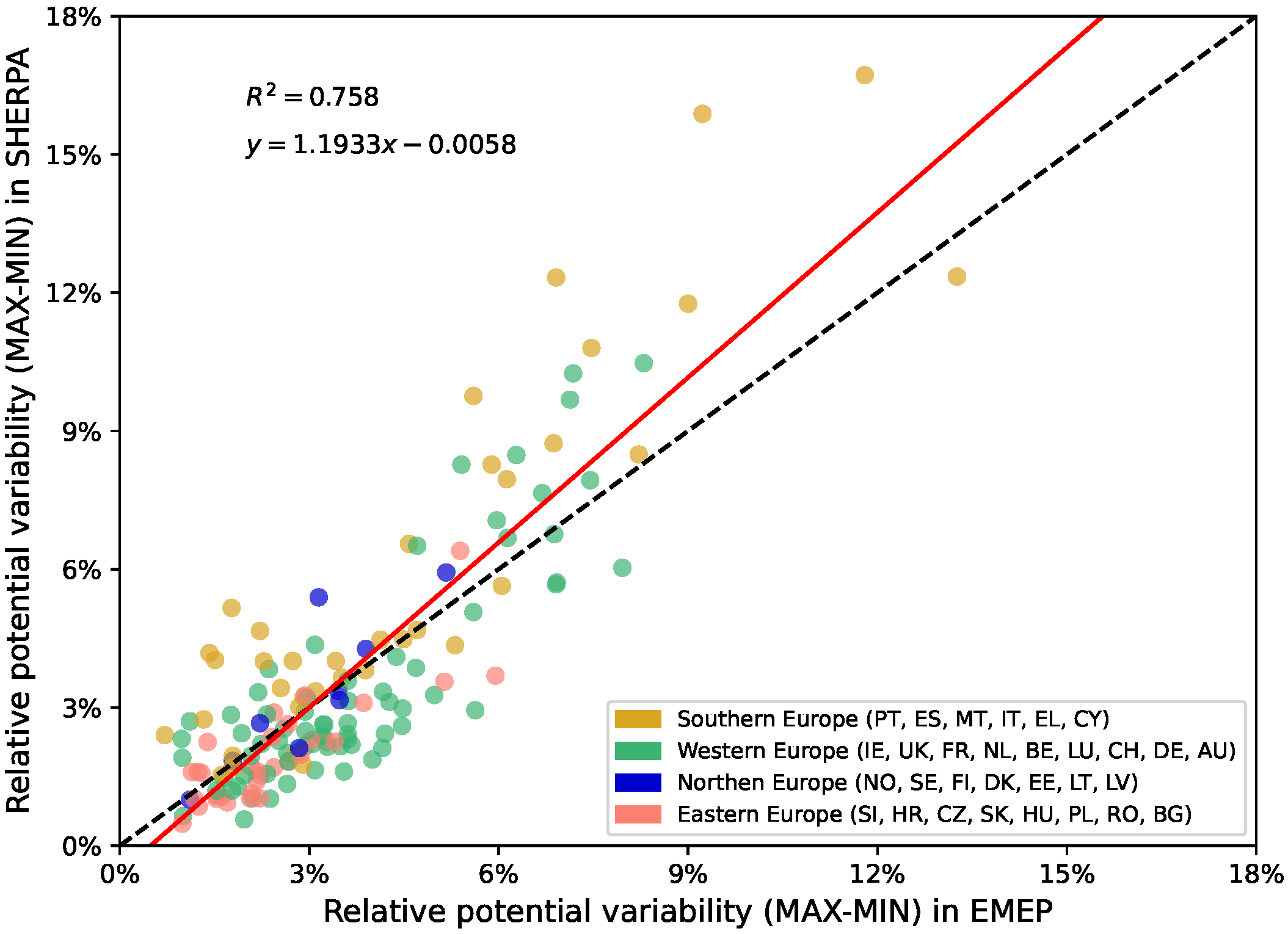
The EMEP Base Case concentrations are similar across the four meteorological years for most urban areas, except for the most polluted ones, where lower concentrations are found in 2015. However, the corresponding absolute ${\mathrm{PM}}_{2.5}$ reduction is also lower in 2015 for these urban areas, leading to relative potentials that are similar in 2015, 2017, 2019, and 2021. As already observed for SHERPA results in Section 3.1, lower potentials are observed in the south of the continent in comparison with the north, with minimal values generally reached in 2015 and maximum values generally reached in 2021. Concerning the meteorological variability in total relative potentials, Figure 7 shows the comparison of inter-annual ranges calculated by SHERPA and obtained from EMEP simulations, highlighting a significant correlation ($R^2=0.758$). This suggests that the two models capture similar variabilities. Here, no significant bias is found and a linear fit between the two variabilities calculates a slope of 1.19. This suggests that for cities where meteorological years differ the most, SHERPA produces a variability slightly higher than that of EMEP simulations. Note that no particular regional or climate group of cities seems to be systematically biased lower or higher by the model. It must be noted that the low variability highlighted by Figure 6 is observed for yearly ${\mathrm{PM}}_{2.5}$ concentrations. However, this variability increases when considering lower averaging times, in particular, during winter months. The comparison of meteorological years for EMEP simulations at the monthly scale can be found in the Supplementary Materials (Figures S7–S9).

Although the main focus of this study is the inter-annual variability of relative potentials, the variability in other meteorological parameters can be studied for completeness. Here, the low variability observed in EMEP can be compared with the variability observed for the main meteorological parameters influencing the distribution of ${\mathrm{PM}}_{2.5}$ in the atmosphere. In the Supplementary Materials (Figure S1), the inter-annual ranges of four air quality parameters are calculated using EMEP outputs: temperature, that accelerates chemical reactions and controls the atmospheric mixing layer; wind speed, which governs pollution dispersion; precipitation, which removes particulate matter and soluble gases from the atmosphere through wet deposition and relative humidity, which affects aerosol formation and hygroscopic growth. Inter-annual ranges of ${\mathrm{PM}}_{2.5}$ concentrations, ${\mathrm{PM}}_{2.5}$ concentration reductions and relative potentials are also calculated. This allows classifying cities in Europe by meteorological variability throughout the four years of the study. A distinction is thus possible between cities where low meteorological variability is associated with low relative potential variability and cities where low relative potential variability occurs despite high meteorological variability, which is not possible with SHERPA alone. For a given city, the corresponding relative potential is considered to have a higher variability if its inter-annual amplitude is greater than the average inter-annual amplitude calculated from the dataset. Similarly, the corresponding meteorology is considered to have a higher variability if at least two of the four meteorological variables above are higher than the mean inter-annual ranges calculated over the dataset. A dual ranking system is applied to the cities, assessing their inter-annual variability in both meteorological parameters and relative potential. This enables the categorization of cities into different groups, including those with stable or variable conditions in one or both of these aspects. Cities in northern, eastern and central Europe appear to have the least variable relative potential, despite more pronounced meteorological variability inland, particularly in terms of temperature and humidity. Cities in the south of the continent, as well as cities in western France and along the Irish Sea, are characterized by higher total relative potential inter-annual ranges. These trends generally agree with the observations provided by Figure 3. However, no regional, large-scale trend is observed for most meteorological parameters. Consequently, the high variability in total relative potentials can only be fully understood through a detailed examination of each city’s specific circumstances. Specific examples of cities are included in the Supplementary Materials (Figure S2) to illustrate all situations. For example, the relative potential of Athina (Greece), lower in 2021 compared to 2015, is largely due to a change in the Base Case concentration between these two years, which can be explained by an intrusion of ${\mathrm{PM}}_{2.5}$ from North Africa. However, the significant differences in precipitation and humidity between these two years may also contribute to this difference. Conversely, the differences in the relative potential of Bordeaux (France) between 2019 and 2021 are largely due to a change in the concentration difference, but the variations in meteorological parameters are also significant, preventing to conclude that emissions are the sole factor of the observed variability. Finally, in Napoli (Italy), all three effects influence the variation of the total relative potential.

The consistency of EMEP results with SHERPA source allocations, and, in particular, the low variability observed for relative potentials for most cities throughout Europe, confirms that SHERPA outputs are not an artifact of the model and reflect CTM simulations. Our results support the use of a single year of simulations to train SHERPA by highlighting the robustness of the source allocation results to meteorological variability, which is critical for policy-making applications.

5. Discussion

This study demonstrates that the EMEP-based SHERPA estimates relative potentials that have a low sensitivity to meteorological variability. However, it is essential to acknowledge that SHERPA is a simplified SRR model, which inherently leads to a slight compromise in accuracy, with errors remaining below 10% [29]. Such bias must be considered in the context of other uncertainties that may impact the results, ultimately affecting the choice of optimal air quality policies. Notably, while the calculated relative potentials exhibit relatively low sensitivity to the input meteorological year, they remain dependent on the corresponding air quality model and reproduce its uncertainties. Past model inter-comparison studies reported substantial differences among models [34]. In the light of these studies, uncertainties attached to the simplified formulation of the tool appear more important than uncertainties linked to meteorological fields. Another source of uncertainty is the emission inventory used as input. Regarding this, Trombetti et al. [35] showed substantial differences between different bottom-up inventories at the urban scale, leading to uncertainties exceeding 100% in some cities and sectors.

Finally, the range of application for SHERPA limits the use of our results. SHERPA results represent yearly averages and do not evaluate the effect of policies on daily or monthly air quality indicators. As a consequence, this tool is not suited to evaluate how air quality policies could help reach EU and WHO guidelines concerning daily exposures. Similarly, since the SHERPA Source-Receptor Relationships are developed based on emission reduction scenarios where emissions are decreased by 50% while assuming a linearity between emission changes and concentration changes below this number, its applicability is limited to scenarios within this range.

6. Conclusions

This study analyzes the sensitivity of source allocation results for ${\mathrm{PM}}_{2.5}$ to meteorological conditions in 150 European cities. Other air pollutants exhibiting different chemical behavior or stronger non-linearities are not studied. Calculations are performed with SHERPA, a Source-Receptor Relationship model. The model is calibrated with a limited number of EMEP simulations and allows analyzing various scenarios of emission reductions. Relative potential of cities in SHERPA outputs is calculated at the scale of the city core, the greater city, the country and Europe, but also for different sectors and precursors. They can be used to determine the optimal scale of action, as well as the priority activity sector and technology to abate emissions and reduce ${\mathrm{PM}}_{2.5}$ exposure for all cities throughout the continent. It is, however, important to assess how robust the relative potentials obtained with one given set of meteorological conditions are. Indeed, it must be ensured that the priority sectors or scales of actions do not change too much when meteorological conditions change. As a consequence, while previous studies have analyzed EMEP-trained SHERPA results for a single meteorological year, four meteorological years were analyzed here to assess the robustness of the tool regarding meteorological variability.

Primary particulate matter appears as the main pollutant driver in Europe. The residential and industrial sectors account for most of the calculated relative potentials at smaller spatial scales, while agriculture and shipping gain importance at larger scales. At the sectoral level, agriculture contributes as much as industry to the variability of the relative potential, while contributing less to its total. At the precursor level, nitrogen oxides and ammonia contribute as much as primary particles to the variability of the relative potential, while contributing less to its total. The relative variability of sectors generally increases with their share within the total relative potential of a city; it is not the case for precursors. Overall, however, relative potentials in Europe remain stable across years and spatial scales, with 9 out of 10 cities having a total relative potential inter-annual range lower than 8%. Notable exceptions concern coastal cities in southern Europe, which are subject to dust intrusions from the Sahara. This low dependence on meteorological input data is not an artifact of the algebraic construction of the SRRs, because similar findings are obtained when using the EMEP model used to drive SHERPA. Moreover, although the use of alternative definitions of receptor points could slightly modify the quantitative estimates for some cities, these overall findings are not expected to change.

This low meteorological variability of relative potentials helps guide targeted air quality policies in Europe. In cities that experience a low variability in absolute concentrations as well, this result increases confidence in the measures applied at the emission level to reduce air pollution. Indeed, in this case, when a calculated reduction in pollutant concentration prevents ${\mathrm{PM}}_{2.5}$ concentrations from exceeding a critical level, then the low meteorological variability in these results ensures that exceedances are effectively avoided regardless of the meteorological conditions. For cities with variable absolute concentrations, however, the implications of this study in terms of policymaking are more nuanced: while SHERPA reliably identifies priority sectors and scales of action, inter-annual variability in background concentrations should be accounted for when designing measures aimed at achieving compliance with air quality standards. Additional attention must also be given to years characterized by extreme events whose magnitude and location differ significantly from those observed during the four years studied. This study, therefore, demonstrates the robustness of the SHERPA tool and shows that training with a small amount of input data corresponding to a single, typical meteorological year could be sufficient to correctly estimate emission reduction impacts. It reinforces the utility of SRR models for the design of policies that aim to reduce ${\mathrm{PM}}_{2.5}$ concentrations and comply with EU and WHO standards.

References

1. European Union. Directive (EU) 2024/2881 of the European Parliament and of the Council of 23 October 2024 on Ambient Air Quality and Cleaner Air for Europe (Recast). OJ L 2024, 20.11.2024. PE/88/2024/REV/1. Available online: http://data.europa.eu/eli/dir/2024/2881/oj (accessed on 28 May 2026).
2. World Health Organization. WHO Global Air Quality Guidelines: Particulate Matter (PM2.5 and PM10), Ozone, Nitrogen Dioxide, Sulfur Dioxide and Carbon Monoxide; World Health Organization: Geneva, Switzerland, 2021. [Google Scholar]
3. European Environment Agency. European Environment Agency: Harm to Human Health from Air Pollution in Europe: Burden of Disease Status, 2024. Briefing No. 21/2024, European Environment Agency. 2024. Available online: https://www.eea.europa.eu/en/analysis/publications/harm-to-human-health-from-air-pollution-2024 (accessed on 28 May 2026).
4. World Health Organization. Economic Cost of the Health Impact of Air Pollution in Europe: Clean Air, Health and Wealth; World Health Organization: Geneva, Switzerland, 2015. [Google Scholar]
5. D’Elia, I.; Bencardino, M.; Ciancarella, L.; Contaldi, M.; Vialetto, G. Technical and Non-Technical Measures for air pollution emission reduction: The integrated assessment of the regional Air Quality Management Plans through the Italian national model. Atmos. Environ. 2009, 43, 6182–6189. [Google Scholar] [CrossRef] [Scilit]
6. Giannouli, M.; Kalognomou, E.-A.; Mellios, G.; Moussiopoulos, N.; Samaras, Z.; Fiala, J. Impact of European emission control strategies on urban and local air quality. Atmos. Environ. 2011, 45, 4753–4762. [Google Scholar] [CrossRef] [Scilit]
7. Amann, M.; Bertok, I.; Borken-Kleefeld, J.; Cofala, J.; Heyes, C.; Höglund-Isaksson, L.; Klimont, Z.; Nguyen, B.; Posch, M.; Rafaj, P.; et al. Cost-effective control of air quality and greenhouse gases in Europe: Modeling and policy applications. Environ. Model. Softw. 2011, 26, 1489–1501. [Google Scholar] [CrossRef] [Scilit]
8. Maas, R.; Grennfelt, P. Towards Cleaner Air; Arctic Monitoring and Assessment Programme: Tromsø, Norway, 2016. [Google Scholar]
9. Simpson, D.; Fagerli, H.; Jonson, J.E.; Tsyro, S.; Wind, P.; Tuovinen, J.-P. PART I Unified EMEP Model Description. In Transboundary Acidification, Eutrophication and Ground Level Ozone in Europe; EMEP Status Report; EMEP: Oslo, Norway, 2003. [Google Scholar]
10. Tuccella, P.; Curci, G.; Visconti, G.; Bessagnet, B.; Menut, L.; Park, R.J. Modeling of gas and aerosol with WRF/Chem over Europe: Evaluation and sensitivity study. J. Geophys. Res. Atmos. 2012, 117, D03303. [Google Scholar] [CrossRef] [Scilit]
11. Szopa, S.; Balkanski, Y.; Schulz, M.; Bekki, S.; Cugnet, D.; Fortems-Cheiney, A.; Turquety, S.; Cozic, A.; Déandreis, C.; Hauglustaine, D.; et al. Aerosol and ozone changes as forcing for climate evolution between 1850 and 2100. Clim. Dyn. 2013, 40, 2223–2250. [Google Scholar]
12. Menut, L.; Bessagnet, B.; Khvorostyanov, D.; Beekmann, M.; Blond, N.; Colette, A.; Coll, I.; Curci, G.; Foret, G.; Hodzic, A.; et al. CHIMERE 2013: A model for regional atmospheric composition modelling. Geosci. Model Dev. 2013, 6, 981–1028. [Google Scholar] [CrossRef] [Scilit]
13. Crippa, M.; Guizzardi, D.; Muntean, M.; Schaaf, E.; Dentener, F.; Van Aardenne, J.A.; Monni, S.; Doering, U.; Olivier, J.G.J.; Pagliari, V.; et al. Gridded emissions of air pollutants for the period 1970–2012 within EDGAR v4.3.2. Earth Syst. Sci. Data 2018, 10, 1987–2013. [Google Scholar] [CrossRef] [Scilit]
14. Granier, C.; Darras, S.; Denier van der Gon, H.; Jana, D.; Elguindi, N.; Bo, G.; Gauss, M.; Guevara, M.; Jalkanen, J.-P.; Kuenen, J.; et al. The Copernicus Atmosphere Monitoring Service Global and Regional Emissions (April 2019 Version); Copernicus Atmosphere Monitoring Service: Reading, UK, 2019. [Google Scholar]
15. Pandolfi, M.; Gonzalez-Castanedo, Y.; Alastuey, A.; de la Rosa, J.D.; Mantilla, E.; De La Campa, A.S.; Querol, X.; Pey, J.; Amato, F.; Moreno, T. Source apportionment of PM10 and PM2.5 at multiple sites in the strait of Gibraltar by PMF: Impact of shipping emissions. Environ. Sci. Pollut. Res. 2011, 18, 260–269. [Google Scholar]
16. Timmermans, R.; Kranenburg, R.; Manders, A.M.M.; Hendriks, C.; Segers, A.J.; Dammers, E.; Zhang, Q.; Wang, L.; Liu, Z.; Zeng, L.; et al. Source apportionment of PM2.5 across China using LOTOS-EUROS. Atmos. Environ. 2017, 164, 370–386. [Google Scholar] [CrossRef] [Scilit]
17. Clappier, A.; Pisoni, E.; Thunis, P. A new approach to design source–receptor relationships for air quality modelling. Environ. Model. Softw. 2015, 74, 66–74. [Google Scholar] [CrossRef] [Scilit]
18. Thunis, P.; Pisoni, E.; Zauli Sajani, S.; Monforti-Ferrario, F.; Bessagnet, B.; Vignati, E.; de Meij, A. Urban PM2.5 Atlas, Air Quality in European Cities; 2023 Report; Publications Office of the European Union: Luxembourg, 2023. [Google Scholar]
19. Organisation for Economic Co-Operation and Development. Redefining “Urban”: A New Way to Measure Metropolitan Areas; Working Party on Territorial Indicators: Paris, France, 2012. [Google Scholar]
20. Simpson, D.; Benedictow, A.; Berge, H.; Bergström, R.; Emberson, L.D.; Fagerli, H.; Flechard, C.R.; Hayman, G.D.; Gauss, M.; Jonson, J.E.; et al. The EMEP MSC-W chemical transport model – Technical description. Atmos. Chem. Phys. 2012, 12, 7825–7865. [Google Scholar] [CrossRef] [Scilit]
21. Denier van der Gon, H.; Kuenen, J.; Visschedijk, A. The TNO CAMS inventories, and alternative (Ref2) emissions for residential wood combustion. In Transboundary Particulate Matter, Photo-Oxidants, Acidifying and Eutrophying Components; EMEP Status Report; The Norwegian Meteorological Institute: Oslo, Norway, 2020; Volume 1, pp. 77–82. [Google Scholar]
22. Kuenen, J.; Dellaert, S.; Visschedijk, A.; Jalkanen, J.-P.; Super, I.; Denier van der Gon, H. CAMS-REG-v4: A state-of-the-art high-resolution European emission inventory for air quality modelling. Earth Syst. Sci. Data 2022, 14, 491–515. [Google Scholar]
23. Tarrason, L.; Fagerli, H.; Jonson, J.E.; Klein, H.; van Loon, M.; Simpson, D.; Tsyro, S.; Vestreng, V.; Wind, P.; Posch, M.; et al. Transboundary Acidification, Eutrophication and Ground Level Ozone in Europe; Norwegian Meteorological Institute: Oslo, Norway, 2004. [Google Scholar]
24. de Meij, A.; Astorga, C.; Thunis, P.; Crippa, M.; Guizzardi, D.; Pisoni, E.; Valverde, V.; Suarez-Bertoa, R.; Oreggioni, G.D.; Mahiques, O.; et al. Modelling the impact of the introduction of the EURO 6d-TEMP/6d regulation for light-duty vehicles on EU air quality. Appl. Sci. 2022, 12, 4257. [Google Scholar]
25. Fagerli, H.; Benedictow, A.; van Caspel, W.; Gauss, M.; Ge, Y.; Jonson, J.E.; Klein, H.; Nyíri, A.; Simpson, D.; Tsyro, S.; et al. Transboundary Particulate Matter, Photo-Oxidants, Acidifying and Eutrophying Components; Norwegian Meteorological Institute: Oslo, Norway, 2023. [Google Scholar]
26. Thunis, P.; Crippa, M.; Cuvelier, C.; Guizzardi, D.; de Meij, A.; Oreggioni, G.; Pisoni, E. Sensitivity of air quality modelling to different emission inventories: A case study over Europe. Atmos. Environ. X 2021, 10, 100111. [Google Scholar] [CrossRef] [Scilit]
27. Degraeuwe, B.; Pisoni, E.; Thunis, P. Prioritising the sources of pollution in European cities: Do air quality modelling applications provide consistent responses? Geosci. Model Dev. 2020, 13, 5725–5736. [Google Scholar] [CrossRef] [Scilit]
28. Thunis, P.; Clappier, A.; Pisoni, E.; Degraeuwe, B. Quantification of non-linearities as a function of time averaging in regional air quality modeling applications. Atmos. Environ. 2015, 103, 263–275. [Google Scholar] [CrossRef] [Scilit]
29. Pisoni, E.; Thunis, P.; Clappier, A. Application of the SHERPA source-receptor relationships, based on the EMEP MSC-W model, for the assessment of air quality policy scenarios. Atmos. Environ. X 2019, 4, 100047. [Google Scholar]
30. Thunis, P.; Degraeuwe, B.; Pisoni, E.; Trombetti, M.; Peduzzi, E.; Belis, C.A.; Wilson, J.; Clappier, A.; Vignati, E. PM2.5 source allocation in European cities: A SHERPA modelling study. Atmos. Environ. 2018, 187, 93–106. [Google Scholar] [CrossRef] [Scilit]
31. United Nations Economic Commission for Europe. Guidelines for Reporting Emissions and Projections Data Under the Convention on Long-Range Transboundary Air Pollution. 2023. Available online: https://unece.org/environment/documents/2022/07/guidelines-reporting-emissions-and-projections-data-under-convention (accessed on 28 May 2026).
32. Thunis, P.; Degraeuwe, B.; Pisoni, E.; Ferrari, F.; Clappier, A. On the design and assessment of regional air quality plans: The SHERPA approach. J. Environ. Manag. 2016, 183, 952–958. [Google Scholar] [CrossRef] [Scilit]
33. Carnevale, C.; Pisoni, E.; Volta, M. A non-linear analysis to detect the origin of PM10 concentrations in Northern Italy. Sci. Total Environ. 2010, 409, 182–191. [Google Scholar] [CrossRef] [Scilit] [PubMed]
34. Pernigotti, D.; Thunis, P.; Cuvelier, C.; Georgieva, E.; Gsella, A.; De Meij, A.; Pirovano, G.; Balzarini, A.; Riva, G.M.; Carnevale, C.; et al. POMI: A model inter-comparison exercise over the Po Valley. Air Qual. Atmos. Health 2013, 6, 701–715. [Google Scholar] [CrossRef] [Scilit]
35. Trombetti, M.; Thunis, P.; Bessagnet, B.; Clappier, A.; Couvidat, F.; Guevara, M.; Kuenen, J.; López-Aparicio, S. Spatial inter-comparison of Top-down emission inventories in European urban areas. Atmos. Environ. 2018, 173, 142–156. [Google Scholar]
Figure 1. Cumulative relative potential for PM 2.5 for the 150 target cities in 2015, 2017, 2019 and 2021 with reduction in the core city (blue), the commuting zone (yellow), the rest of the corresponding country (green) and the rest of Europe (red). How to read the figure: “In Palermo (third row), reducing emissions in the city core only reduces PM 2.5 exposure by between 8% and 9%, while reducing them at the scale of the greater city reduces it by 11% to 13%. Reducing emissions in the entire country will reduce this exposure by 22% to 26%, and reducing the in all of Europe will reduce it by 43% to 52%”.
Atmosphere 17 00641 g001
Figure 2. Number and share of cities in the target group by reached cumulative relative potential for PM 2.5 , with reduction in the core city (blue), the commuting zone (yellow), the rest of the corresponding country (green) and the rest of Europe (red). Shaded areas represent variations of the reached relative potential between years (2015, 2017, 2019 and 2021), while mean relative potentials for the four years are denoted with black lines. How to read the figure: “To reduce exposure to PM 2.5 by at least 20%, reducing emissions in the city core only is enough for 78 to 79 of the target cities, reducing emissions in the corresponding functional urban area (greater city) will be enough for 129 to 131 of the target cities, reducing emissions in the entire corresponding country will be enough for 147 of the target cities, and reducing European emissions will be enough for all target cities”.
Atmosphere 17 00641 g002
Figure 3. Cumulative variability between years 2015, 2017, 2019 and 2021 (maximum minus minimum relative potential) by scale of reduction in 150 target cities. The final variability, i.e., for emission reductions in Europe, is represented by the total size of the bar. Negative values represent spatial scale reductions that reduce the relative potential variability between the four meteorological years. How to read the figure: “In Montpellier (8th row), the inter-annual range of the relative potential for an emission reduction performed in the city core is about 1%. Extending the emission reduction to the greater city increases this range to about 2%. Extending further the emission reduction to the corresponding country (France) increases the inter-annual range to a bit more than 6%, and extending it to the entire Europe increases this range to more than 10%. In Nottingham (132nd row), the inter-annual range of the relative potential for an emission reduction performed in the greater city is slightly less than 3%, but extending the emission reduction to the country (United Kingdom) or to Europe would reduce this range by more than 1%.”
Atmosphere 17 00641 g003
Figure 4. 4-year mean relative potential for different reduction scales (clockwise from top left corner: city core, greater city, country and Europe), with the share of the first three dominant emission sectors. For each point, the three sectors with the lowest share in the total relative potential are gathered and represented in grey.
Atmosphere 17 00641 g004
Figure 5. 4-year mean relative potential for different reduction scales (clockwise from top left corner: city core, greater city, country and Europe), with the share of the first three dominant emission precursors. For each point, the three precursors with the lowest share in the total relative potential are gathered and represented in grey.
Atmosphere 17 00641 g005
Figure 6. Comparison of 2015 with other meteorological years 2017, 2019 and 2021 in EMEP simulations for Base Case PM 2.5 concentration (left), absolute PM 2.5 concentration reduction (middle) and relative potential (right). The evaluation is performed for the receptor point (the point with the highest concentration) of each city in the 150 cities set. The black dotted lines corresponds to the 1:1 diagonal.
Atmosphere 17 00641 g006
Figure 7. Comparison of EMEP outputs and SHERPA results for cumulated variability of the relative potential between years 2015, 2017, 2019 and 2021 (maximum minus minimum relative potential) for all cities. The color of each point corresponds to the subregion of the corresponding city. The red line corresponds to the best linear fit between the two variables and the black dotted line is the 1:1 diagonal.
Atmosphere 17 00641 g007