A Hybrid Statistical-Machine Learning Framework for Risk-Based Screening of High-Frequency Carbon Emission Data Under Emissions Trading Systems

Abstract

Reliable carbon emission data are essential for the effective operation of emissions trading systems (ETS), especially as China’s ETS expands to include energy-intensive industries. This study proposes a hybrid, risk-based anomaly detection framework for high-frequency CO₂ emission data by cross-validating material-based emissions with flue gas-based monitoring data. Under normal operating conditions, the ratio of material-based to flue gas-based emissions is expected to remain within a relatively stable distribution. Potential high-risk periods can therefore be identified when this relationship is distorted or when local temporal patterns deviate from expected behavior. The framework combines Hartigan’s dip test with a window-based Random Forest (RF) classifier, which is suitable for continuous monitoring data that may exhibit temporal dependence. The framework was evaluated using 15-min CO₂ emission data from a cement production facility, with simulations of anomaly magnitude, duration, and mode. Results show that the dip test performs well for long-lasting or strong anomalies, whereas the RF model is more sensitive to subtle, short-term deviations. In the integrated framework, 94.7% of anomalous periods were detected by at least one method and flagged as potential data-quality risks, whereas normal periods were not flagged, supporting its use to prioritize verification efforts.

1. Introduction

The cement industry plays a critical role in global economic development. Presently, this industry accounts for about 7–8% of global carbon emissions [1]. China alone produces 55% of the world’s cement [2]. Despite continuous improvements in energy efficiency, energy consumption in China’s cement industry remains high, and its efficiency still lags behind that of many developed countries [3]. Improving the reliability of carbon emission monitoring in this sector is therefore essential for supporting its low-carbon transition.

The carbon emissions trading system (ETS) has been widely recognized as an effective market-based instrument for mitigating greenhouse gas (GHG) emissions and promoting low-carbon transitions [4,5,6]. Following the official launch of China’s national ETS in July 2021, the regulatory scope has continued to expand. In 2025, the cement industry, together with steel and aluminum smelting industries, was formally included in the national carbon market, adding approximately 1500 regulated entities and covering nearly 8 billion tons of CO₂ emissions annually [7,8]. This rapid expansion substantially increases regulatory demands on emission monitoring, reporting and verification (MRV), posing new challenges for environmental management authorities.

High-quality emission data form the foundation of an effective ETS, directly affecting market integrity, allowance allocation fairness, and the credibility of compliance assessment [9,10]. At present, internationally recognized greenhouse gas quantification methods are categorized into calculation-based and measurement-based approaches, the latter of which includes the continuous emission monitoring system (CEMS) [11]. China’s current ETS reporting framework relies on calculation-based accounting methods. These methods often depend on emission factors, activity data, and manual data inputs, which may not fully capture enterprise-specific variability and may increase the risk of reporting inconsistencies. In contrast, the CO₂-CEMS continuously measures the CO₂ concentration and flue gas flow rate, offering a higher level of automation compared to the calculation-based methods. However, complex flow fields in the flue gas duct make accurate measurement of flow-rate parameters challenging, which can introduce systematic errors and affect the accuracy of monitoring data [12,13,14,15]. These uncertainties underscore the need for risk-based data quality screening. As the ETS expands to cover more sectors and facilities, reliance on labor-intensive manual verification becomes increasingly costly and difficult to scale, further highlighting the need for efficient, data-driven regulatory screening tools.

Recent studies have explored data-driven approaches to improve emission data quality under ETS frameworks [9,16,17]. For example, Yu et al. (2023) compared multiple supervised and unsupervised machine learning methods to identify anomalies in enterprise-level emission data [17]. While such approaches demonstrate promising potential, existing studies have largely focused on annual or low-frequency emission data, with validation typically conducted on an annual basis. More recently, Jia et al. developed a statistical framework for screening the quality of high-frequency emission data in the power industry by cross-validating calculation-based emissions derived from actual coal consumption against flue gas-based emissions [18]. In that framework, the ratio of the two emission estimates was used as a process-level indicator, and deviations from its statistical distribution were interpreted as potential data quality risks. Statistical hypothesis tests, including tests of mean, variance, and non-parametric distributional characteristics, were applied to support risk-based screening.

Building on this cross-validation concept, the present study further addresses the use of high-frequency emission data in continuous regulatory screening. In real industrial monitoring systems, high-frequency flue gas-based measurements are generated as continuous time series rather than independent random observations. Emissions at a given time point may be influenced by previous process states because of system inertia and residence time. Therefore, method selection for continuous screening should account for both distribution-level changes and local temporal anomaly patterns. Purely machine learning-based approaches may achieve high detection accuracy but often provide limited interpretability for regulatory applications. Conversely, statistical approaches provide transparent global diagnostics and are attractive for regulatory applications, but their practical use in continuous industrial time-series data remains challenging. There remains a need for integrated frameworks that align anomaly detection with real-world regulatory workflows, particularly under high-frequency, multi-source monitoring conditions.

To address these challenges, this study develops a hybrid, data-driven framework for anomaly detection and verification of emission data in the context of ETS. Hartigan’s dip test was selected as the statistical component because it evaluates changes in distributional shape, particularly departures from unimodality, and therefore provides an interpretable diagnostic of emission-ratio distortion. A window-based Random Forest model was further introduced to capture local temporal patterns associated with short-duration or low-magnitude anomalies. By integrating these two complementary methods, the proposed framework combines distribution-level and window-level evidence and translates the detection outputs into an interpretable risk score for regulatory review.

The main contributions of this study are threefold. First, a cross-validation framework integrating material-based and flue gas-based emission data is proposed to enhance data quality management in ETS-regulated industrial sectors. Second, a hybrid anomaly detection strategy is developed by combining a global, distribution-based statistical test with a local, window-based machine learning model, thereby aligning anomaly detection with practical regulatory screening needs. Third, using high-frequency emission data from a cement production facility, the detection performance of the proposed framework is systematically evaluated under varying anomaly magnitudes, durations, and modes, demonstrating that the combined approach improves screening effectiveness while maintaining a low false-positive rate. Although demonstrated using data from the cement industry, the proposed framework is potentially adaptable to other energy-intensive sectors covered by ETS, providing a scalable and interpretable tool for regulatory authorities to prioritize verification efforts under limited resources.

2. Materials and Methods

2.1. Data Collection

This study integrated carbon emission data from material- and flue gas-based monitoring to develop a data quality diagnostic framework based on their cross-relationships. High-frequency data were collected from a cement production facility in southern China that operates a dry-process production line with a designed clinker capacity of 5000 tons per day. The data collection period extended from 12 October to 12 December 2024. Data gaps between 30 October and 5 November 2024, were attributed to temporary equipment malfunctions and excluded from subsequent analysis.

For flue gas-based monitoring, CO₂ emissions were measured using a CEMS installed at a 40-m platform on a 90-m kiln stack. The monitoring point was located at a distance of at least four equivalent diameters downstream of the upstream flow disturbance, i.e., the gas inlet. Instruments for measuring CO₂ concentration, flow rate, humidity, temperature and static pressure were manufactured by Sick Maihak (Waldkirch, Germany). The installation strictly followed national technical specifications for pollutant CEMS [19].

Material-based emissions were calculated following the Guidelines for Accounting and Reporting of Corporate Greenhouse Gas Emissions—Cement Industry (CETS-AG-02.01-V01-2024) issued by China’s Ministry of Ecology and Environment [20]. Combustion emissions were estimated from second-resolution coal consumption data recorded by rotor scales at the kiln inlet and precalciner, combined with carbon content per unit calorific value and daily measurements of coal lower heating values. Process emissions were calculated based on raw meal consumption measured by the Schenck scale prior to the kiln, clinker production estimates and default emission factors [20]. Detailed calculations are presented in Text S1 in the Supplementary Information. During the data collection period, no alternative fuels or high-carbon-content alternative raw materials were used.

2.2. Data Pre-Processing

The goal of data pre-processing was to obtain 15-min-interval carbon emissions from both material-based and flue-gas-based monitoring. The data collected in Section 2.1 were first cleaned at the second level to remove data recorded during instrument maintenance and calibration of the flue gas-based monitoring system. Second-level carbon emissions for both material-based and flue-gas-based monitoring were calculated after data cleaning. The core of this study was a combined monitoring method that relied on both material- and flue-gas-based data for data-quality diagnosis. Therefore, if carbon emission data from either the flue gas or material monitoring method was missing or abnormal at any given time, the corresponding data from the other method for the same period was also considered invalid. After data cleaning, the second-level emission data were aggregated at 15-min intervals.

2.3. Operation Condition Classification and Emission Ratio Calculation

Operational conditions were classified based on clinker production load, which represented the primary source of variability during the study period. From 22 October to 20 November 2024, the average clinker production rate was approximately 4940 tons per day, whereas production during the remaining periods averaged about 6480 tons per day. Accordingly, two operating conditions (OC) were defined: OC1 (high production load) and OC2 (low production load). The emission ratio $R_{i,j}$ represents the ratio of carbon emissions measured through material-based monitoring to those measured through flue gas-based monitoring over a 15-min interval. The calculation formula is as follows:

$$R_{i,j}={\displaystyle \frac{E_{mb,i,j}}{E_{fb,i,j}}}$$

(1)

where:

$E_{mb,i,j}$ and $E_{fb,i,j}$ are the material-based and flue gas-based emissions for the $i$-th operational condition at the $j$-th 15-min interval, respectively. This ratio was used because it provides a normalized indicator for cross-validating the two independent monitoring approaches under the same operating conditions.

2.4. Development of a Data Quality Diagnostic Framework

2.4.1. Reference and Testing Periods

For each operating condition, emissions were ordered chronologically and divided into a reference (train) period and a testing period. The first 70% of the data were used as the reference dataset for the statistical method and as the source data for constructing the RF training dataset. The remaining 30% constituted the testing period, into which synthetic anomalies were introduced for performance evaluation. Unlike random sampling-based validation, this chronological split was adopted to approximate practical regulatory deployment, in which historical monitoring data are used to screen subsequent reporting periods. Preserving temporal order also allowed the framework to evaluate anomaly detection under realistic time-series conditions, where reference and testing periods may not be perfectly exchangeable because of operational variability or temporal drift.

2.4.2. Simulation of Anomalies

Synthetic anomalies were used for two purposes: to construct labeled anomalous windows for RF training (for the machine learning approach) and to evaluate detection performance in the testing period (for both statistical and machine learning approaches). Key material-related variables, including coal consumption, raw meal consumption, material-based CO₂ emissions, and emission ratios, were modified. Anomaly magnitude (β) was varied from 0.02 to 0.30 to represent different levels of reporting inconsistency, while anomaly duration ranged from 0.5 to 8 days to simulate both short-term errors and sustained misreporting.

Three anomaly modes were considered: scale (uniform level shift), flat (suppressed temporal variability), and ramp (gradual deviation followed by recovery). Each anomaly scenario was simulated 50 times with randomly selected starting positions to account for stochastic variability, with only one continuous anomaly event introduced per testing period. The synthetic anomalies were designed to mimic plausible reporting distortions and were used to conduct a controlled methodological evaluation. However, they may not fully represent the complexity and diversity of real-world reporting errors or verified compliance violations.

2.4.3. Statistical Detection Method

Hartigan’s dip test was applied to detect departures from unimodality in the emission ratio distribution. Under normal operating conditions, emission ratios are assumed to follow an approximately unimodal distribution for a given operating condition, while anomalies can distort the original distribution to multimodality (the distribution change after anomaly injection is shown in Figure S1 in the Supplementary Information). For each simulated anomaly scenario, emission ratio data from the 70% clean reference period and the 30% testing period with injected anomalies were concatenated, and the dip test was applied to the combined empirical distribution. Because the dip test was used as a preliminary screening tool rather than a conventional hypothesis test for statistical inference, α was interpreted as a screening threshold. A relatively high α threshold of 0.75 was adopted to reduce false negatives, consistent with the priority of risk-based regulatory screening. To evaluate the influence of this threshold choice, a sensitivity analysis was conducted using α values from 0.05 to 0.90, with changes in the true positive rate (TPR) and false positive rate (FPR) assessed under simulated anomaly scenarios and clean testing data, respectively. The detailed results are provided in the Supplementary Information (Figure S2 in the Supplementary Information). The anomaly simulation was repeated 50 times with randomly selected starting positions to account for stochastic variability, and the event-level TPR was calculated using Equation (2). TPR was used because the objective of this study was preliminary risk screening, where reducing missed anomalous periods is important.

$$TPR={\displaystyle \frac{TP}{TP+FN}}$$

(2)

where

$TP$: True positive, represents the number of actual positive samples that were correctly identified as positive.

$FN$: False negative, represents the number of actual positive samples that are incorrectly classified as negative.

2.4.4. Machine Learning-Based Detection Method

In this study, RF was used as a supervised binary classifier, where each window was classified as either normal or anomalous. Both clean data and data with simulated anomalies were used as training data, and the trained model learned feature patterns that distinguish normal windows from anomaly-containing windows, then classified each new window as normal or anomalous. The RF classifier was implemented with 200 trees, no maximum tree-depth constraint, balanced class weights, and bootstrap aggregation using the default settings in scikit-learn. The random seed was fixed for reproducibility.

Time series data were segmented into overlapping window sizes (W) of 24, 48, 96 and 192 data points, corresponding to 6, 12, 24, and 48 h, respectively, with a stride equal to half the window length. For each window size, statistical and dynamic features were extracted, including mean, standard deviation, minimum, maximum, slope and first-order differences of the key variables.

To construct the training dataset, clean windows from the reference period were labeled as normal, while windows containing simulated anomalies were labeled as anomalous. Three anomaly modes were introduced into the training data to represent different types of data quality problems: (i) scale mode (uniformly scaling relevant material and emission variables); (ii) flat mode (flattening temporal variation within a window); and (iii) ramp mode (involving gradual deviation from the baseline (ramp-down), a sustained abnormal level (hold), and a gradual return to normal (ramp-up)). The RF classifier was then trained using the extracted window-level features and binary labels.

After training, the model was applied to the testing period. For each testing window, the same set of features was extracted and input into the trained RF classifier. The model generated an anomaly probability for each window, and windows with predicted probabilities greater than 0.5 were classified as anomalous. In this way, the RF model converted continuous high-frequency monitoring data into a sequence of window-level anomaly labels. Each combination of anomaly mode, duration, and magnitude was simulated 50 times with different starting positions, with only one anomaly event introduced per repetition.

Detection performance was evaluated at both the window level and the event level. Window-level TPR was calculated as the proportion of anomaly-containing windows correctly classified as anomalous. Event-level TPR was used to evaluate whether a continuous anomaly event was detected. An event was considered detected if the proportion of anomalous windows identified within the event period exceeded the baseline false-positive rate obtained from clean testing data. This event-level criterion was used to reflect the practical objective of identifying anomalous reporting periods rather than isolated data points. F1-score, FPR, ROC-AUC, and the confusion matrix were calculated for the selected window setting (W = 48, stride = 24). For this evaluation, anomaly-containing windows from all simulated scenarios were pooled as positive samples. Clean windows were extracted from windows with no anomalous points and deduplicated based on window start and end positions to avoid counting the same clean testing windows across simulation repetitions.

Feature importance and SHAP analysis were further calculated from the trained RF model to identify the variables and window-level statistics that contributed most to anomaly discrimination.

2.4.5. Integrated Framework and Risk Scoring

To support risk-based regulatory screening, outputs from the statistical and machine learning methods were integrated into a simple, interpretable risk score. For each anomaly event, binary indicators were assigned based on detection by the dip test and the RF model. For the i-th anomaly event, two binary indicators were defined:

$$D_i^{Dip}=1\mathrm{if}\mathrm{the}\mathrm{dip}\mathrm{test}\mathrm{detected}\mathrm{an}\mathrm{anomaly},and0\mathrm{otherwise}.$$

(3)

$$\begin{gathered} D_i^{RF}=1\mathrm{if}\mathrm{the}\mathrm{RF}\mathrm{model}\mathrm{detected}\mathrm{the}\mathrm{anomaly}\mathrm{event}\mathrm{based}\mathrm{on}\mathrm{the}\mathrm{window}\text{-} \\ \mathrm{level}\mathrm{classification}\mathrm{results},\mathrm{and}0\mathrm{otherwise}. \end{gathered}$$

(4)

The risk score (${Risk}_i$) was then calculated as

$${Risk}_i=D_i^{Dip}+D_i^{RF}$$

(5)

The score (${Risk}_i$) was defined as the sum of the two binary detection indicators. It represents the number of independent detection signals, with a higher score indicating a higher priority for regulatory review.

2.5. Framework Overview

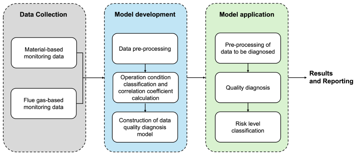
Figure 1 illustrates an overview of the proposed anomaly detection framework. By combining material-based and flue gas-based emission data, this framework is designed to support regulatory screening and enhance the efficiency of carbon emission verification processes. A detailed method workflow of the hybrid screening framework is illustrated in Figure S3 of the Supplementary Information.

3. Results

3.1. Emission Data Characteristics Under Different Operating Conditions

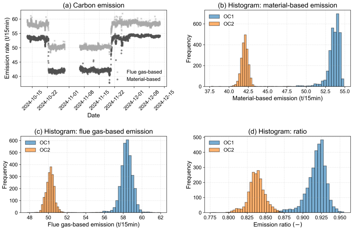
The second-level data collected during this experiment were used to calculate 15-min carbon emissions using the accounting method. As shown in Figure 2a, the overall trends in carbon emissions from both flue gas-based monitoring and material-based monitoring were consistent. However, the carbon emissions measured by flue gas monitoring were higher than those measured by material-based monitoring. Specifically, during the high production load period (OC1), the flue gas method was approximately 8% higher than the material method, whereas during OC2 (low production period), it was 16% higher.

Figure 2b–d present histograms of carbon emissions from material-based monitoring, flue gas-based monitoring, and their ratio. Both carbon emissions and the ratio exhibit two distinct peaks (one orange and one blue) under the two operating conditions. When performing a Kolmogorov-Smirnov (K-S) normality test on each orange or blue distribution, the carbon emissions from material-based monitoring under both OC1 and OC2 did not follow a normal distribution, as shown in Figure 2b. Similarly, the flue gas-based emissions and ratios under OC1 and OC2 were also non-normally distributed (Figure 2c,d). This could be attributed to the relatively short data-collection period, which may not have captured enough data points, and to the inclusion of transition states in the dataset.

Unimodality testing was conducted separately for OC1 and OC2. The material-based emissions failed the dip test under both operating conditions (Figure 2b), indicating departures from unimodality. In contrast, the flue gas-based emissions and emission ratios passed the dip test under both OC1 and OC2 (Figure 2c,d), suggesting approximately unimodal distributions within each operating condition. The primary reason for this discrepancy may be that the material monitoring method relied on coal consumption and raw meal consumption, which were process-control parameters that exhibit small, range-limited fluctuations, leading to a multimodal distribution. On the other hand, flue gas monitoring measures the overall system’s carbon emissions under relatively stable operating conditions, resulting in more consistent data and a unimodal distribution. The emission ratio, being the ratio of material-based to flue gas-based emissions, also followed a unimodal distribution. Song et al. (2024) also reported that under different operating conditions (e.g., varying boiler start/stop states), the ratio of carbon emissions from flue gas-based monitoring to material-based monitoring in a power plant followed a unimodal distribution [14]. This unimodality of datasets can be further used to detect anomalies, as shown in Section 3.2.

3.2. Performance of Unimodality-Based Statistical Detection

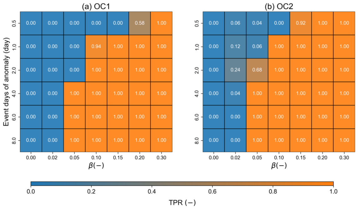
The statistical method employed in this study was the dip test, which evaluated whether the combined reference and testing datasets follow a unimodal distribution. When the reference and testing datasets originate from the same distribution, the combined dataset is expected to exhibit unimodality. Conversely, deviations from unimodality indicate the potential presence of anomalous data within the testing set. Figure 3 illustrates the TPR when artificial anomalies were introduced into the testing set with continuous perturbations at varying levels of simulated anomaly magnitude.

When the anomaly magnitude (β) was 0, the TPR was 0 under both operating conditions, reflecting a zero false positive rate. As both the anomaly magnitude and event days of anomaly increased, the TPR generally rose. Specifically, both OC1 and OC2 exhibited a TPR of 1 when the number of event days of simulated anomaly exceeded 1 day, and the anomaly magnitude exceeded 0.1. Similarly, if the anomaly magnitude was greater than or equal to 0.05 and the number of event days exceeded 4, the TPR reached 1. Notably, the TPR for OC2 was the same or higher than that for OC1.

3.3. Detection Performance of the RF-Based Approach

In this study, an RF model was developed using a sliding-window approach, which detects sequences of anomalies rather than individual points. While general data anomalies may occur as isolated points, this study assumes that non-random anomalies in carbon market data are less likely to appear as single-point deviations and more likely to manifest as temporally continuous abnormal periods. The model tested six different anomaly durations, which is the same as in the statistical method. Each anomaly event may consist of one or more windows. Four different window sizes (W) were tested for model performance. The proportion of anomalous data within a window ranged from 0 to 1 and was defined as the contamination ratio.

3.3.1. Effects of Contamination Ratio and Window Size on RF Detection Performance

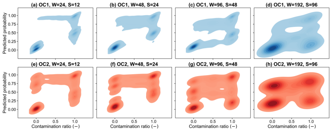
Figure 4 shows two-dimensional kernel density estimation (2D KDE) plots of contamination ratio versus RF-predicted anomaly probability for different window sizes under the two operating conditions. The contamination ratio represents the proportion of anomalous data points within a window. Windows with predicted probabilities greater than 0.5 were classified as anomalous.

Overall, the predicted anomaly probability increased with contamination ratio under both operating conditions, indicating that the RF model was generally more likely to identify windows with higher anomaly content. However, the relationship was influenced by window size. For both OC1 and OC2, the separation between low- and high-probability regions became clearer as the contamination ratio increased.

The results also show that smaller window sizes did not always lead to better detection performance. In particular, W = 48 generally produced more stable probability separation than W = 24, especially when the contamination ratio was high. In contrast, larger window sizes (W = 96 and W = 192) exhibited broader probability distributions across certain contamination-ratio ranges. These results suggest that RF detection performance depends on both contamination ratio and window size, and that an intermediate window size may provide a better balance between local sensitivity and detection stability. Moreover, the contamination ratio was used as a post hoc evaluation variable to analyze how the proportion of anomalous points within a window affected RF detection performance. It was not used as an input feature of the RF model or as a decision threshold in practical screening. A detailed interpretation of the probability patterns is provided in Text S2 of the Supplementary Information.

3.3.2. Detection Performance Across Anomaly Magnitudes and Modes

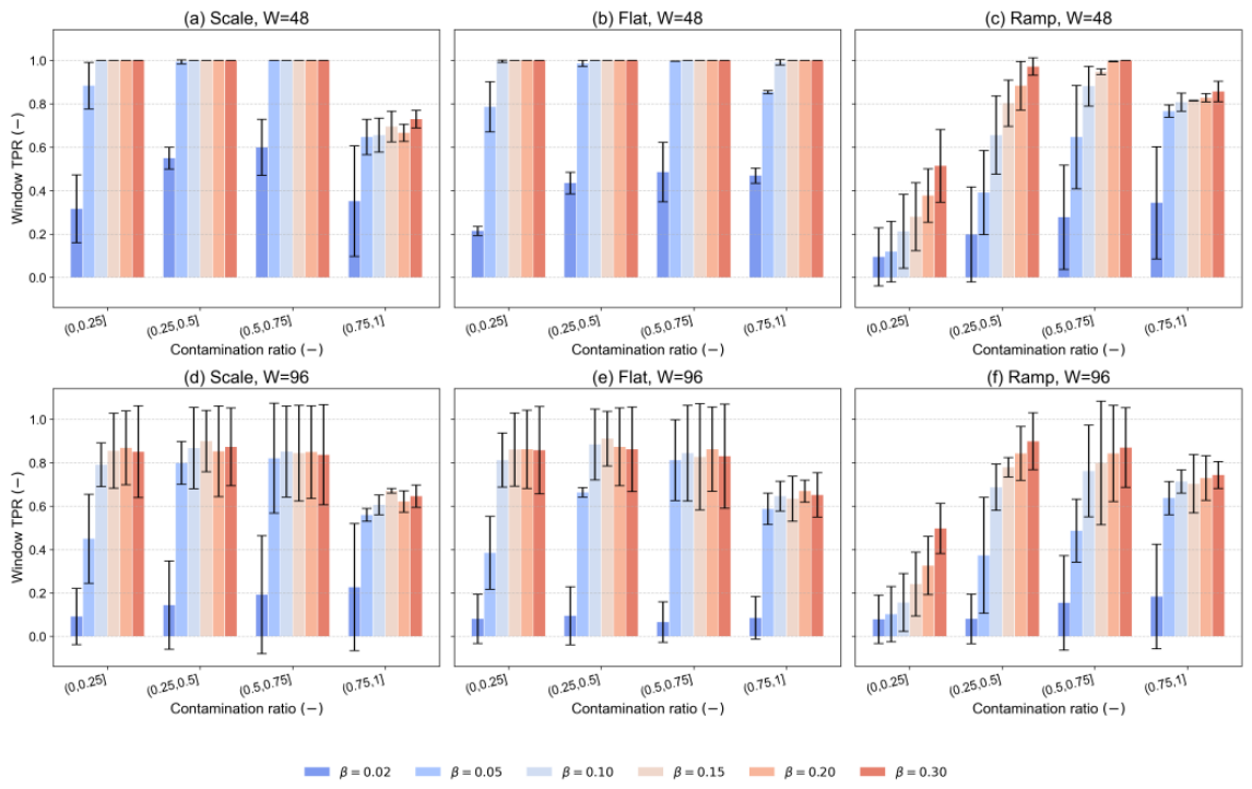
Figure 5 illustrates the model’s performance for window sizes W = 48 and W = 96. Results for W = 24 and W = 192 are provided in Figures S4 and S5 in the Supplementary Information. The figure highlights the sensitivity of window TPR performance to different values of β and anomaly modes, as well as the influence of varying contamination ratios. First, the impact of β was analyzed. Regardless of the anomaly mode or window size, the window TPR increased as β increased. The window TPR reached its maximum at β = 0.15 in the Scale and Flat modes.

Next, the effect of contamination ratio on window TPR was considered. As the contamination ratio increased from (0–0.25] to (0.5–0.75], the window TPR changed only slightly. When the contamination ratio increased to the range of (0.75–1], the TPR decreased for all three modes compared to lower contamination ratios, with the most significant decline observed in the scale mode. In the scale mode, changes in the emission series were mainly reflected in the window-level mean. At the same time, other statistical features, including standard deviation, slope, and first-order difference, remained largely unchanged. Accordingly, the model’s detection performance was reduced under this anomaly mode. Moreover, the reduced TPR in the highest contamination-ratio bin may partly reflect the fact that fully contaminated windows contain fewer clean-anomaly transition features than boundary windows. Since the RF model relies on window-level features such as mean, standard deviation, slope, and first-order differences, boundary windows may sometimes provide stronger local-change signals than windows that are entirely covered by a relatively stable anomalous period.

3.3.3. Effects of Anomaly Duration on Window-Level and Event-Level TPR

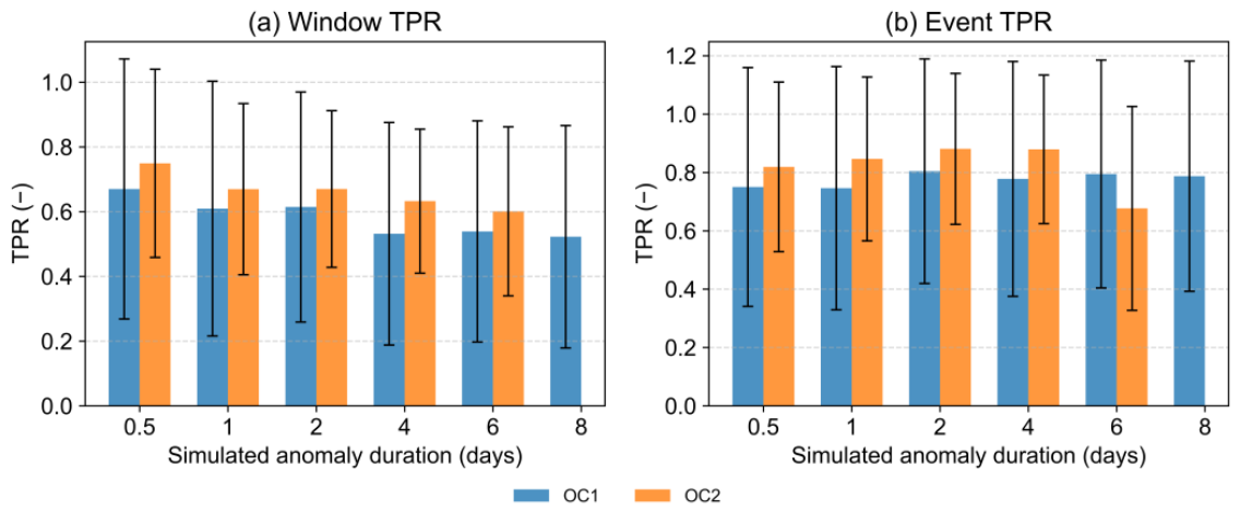
This section compares the impact of the duration of continuous anomalous data (event days of anomaly) on window TPR and event TPR. As shown in Figure 6a, the window TPR gradually decreases as the number of event days of anomaly increases. As the number of anomaly event days increases, the number of data points with a contamination ratio of 1 rises, since only the beginning and end of the event may have windows with a contamination ratio less than 1. As discussed previously, when the contamination ratio is 1, the window TPR is lower. In contrast, the event TPR shows little change as the event days of anomaly increase (Figure 6b). This suggests that increasing the number of anomalous days does not significantly improve the TPR for a given anomaly event.

Additional window-level performance metrics were calculated for the selected window setting (W = 48, stride = 24) (Table S1). After pooling both operating conditions, the RF model achieved a precision of 0.9999, recall/TPR of 0.6977, F1-score of 0.8219, FPR of 0.1148, and ROC-AUC of 0.9330. The additional metrics provide a more complete characterization of RF performance.

3.3.4. Feature Contribution Patterns Under Different Operating Conditions and Window Sizes

Understanding feature contribution is important for identifying which statistical descriptors and monitoring variables most strongly influence the RF model, especially for environmental management and regulatory screening. In this study, two complementary approaches were used: impurity-based RF feature importance was first used to examine the variables and statistical features most frequently used by the trained models, while SHAP analysis was further applied to evaluate the robustness and interpretability of feature contributions across two operating conditions and four window sizes.

The impurity-based feature importance results showed clear differences between the two conditions. For OC1, the window mean was the most important statistical feature across all window sizes, followed by standard deviation (Std) and minimum value (Min) (Figure S6). In contrast, OC2 assigned the highest importance to the minimum value, followed by the mean and the standard deviation. This suggests that OC1 anomalies were mainly detected through changes in the overall level and within-window fluctuations, whereas OC2 relied more on lower-bound changes and average levels. The consistent rankings across window sizes indicate that these patterns are relatively robust. At the variable level, clinker production, material-based CO₂ emissions, and emission ratios were the most influential variables in both conditions.

SHAP analysis further supported these RF feature importance results. Across the two operating conditions and four window sizes, clinker production, coal consumption, material-based CO₂ emissions, emission ratios, and flue gas-based CO₂ emission rate consistently appeared among the most important predictors (Figure S7). SHAP also showed that mean and minimum values were the most stable statistical descriptors, while maximum and standard deviation contributed in several settings (Figure S7). By comparison, slope and first-order difference generally had lower contributions, suggesting that the model was more sensitive to changes in signal level and range than to short-term directional trends.

These importance patterns are partly related to the simulated anomaly modes, as scale, flat, and ramp manipulations directly affect signal levels, extrema, and variability. Nevertheless, these modes were designed to reflect plausible data-quality problems in practical monitoring, such as systematic underreporting, flattened signals, and gradual deviations. Therefore, the RF feature importance and SHAP results remain useful for interpretability in real-world regulatory screening. However, the relative importance of specific features may vary under other operational or sensor-related anomalies.

3.4. Performance of the Combined Detection and Risk Scoring Framework

The combined detection framework integrates statistical testing and RF-based classification to support risk-based regulatory screening of emission data. Instead of relying solely on binary detection outcomes, the framework assigns a discrete risk score to each period that reflects the joint evidence from the two detection methods. A window size of 48 data points was set in the combined detection framework since it demonstrated optimal performance in this study, as mentioned in Section 3.3.1.

The distribution of risk scores clearly separates anomalous from normal periods (

Table 1. Risk score distribution.

	Risk = 0	Risk = 1	Risk = 2
Anomalous periods	5.3%	22.5%	72.2%
Normal periods	100%	0%	0%

). As summarized in the risk score results, 94.7% of anomalous periods are assigned Risk = 1 or Risk = 2, with 72.2% in the highest-risk category (Risk = 2). In contrast, all normal periods were assigned Risk = 0, indicating a low tendency for false alarms. This pronounced contrast indicates that the risk score provides an effective basis for regulatory screening while maintaining a low false-alarm tendency.

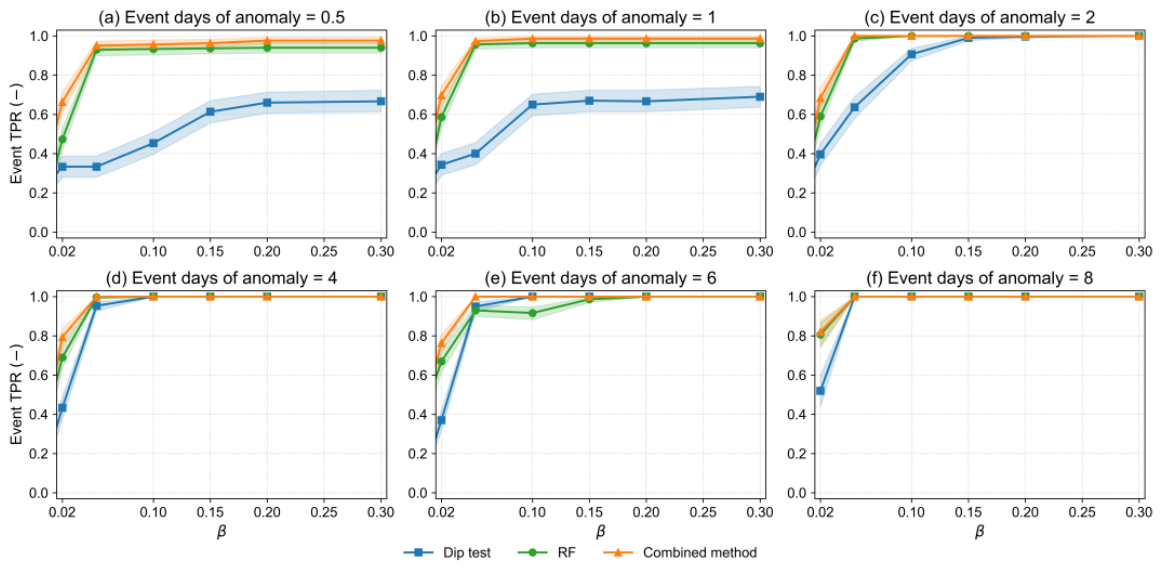
Based on these results, Risk ≥ 1 is adopted as the screening threshold for anomaly detection. Under this threshold, most anomalous periods are successfully captured, while normal periods are rarely misclassified. Figure 7 presents the detection performance under the risk-based decision rule, illustrating event-level TPR as a function of anomaly magnitude (β) and event duration. The shaded areas indicate 95% bootstrap confidence intervals. Another figure showing the mean event-level TPR with ±1 standard deviation is provided in Figure S8 of the Supplementary Information. When anomalous events were short (e.g., 0.5 or 1 day), the RF-based method exhibited higher sensitivity, particularly at lower β values. As the event duration increased, the detection performance of the statistical and RF-based methods gradually converged.

The combined approach, in which an event was classified as anomalous if detected by either method, achieved higher TPR values at lower β levels. Undetected anomalous events (Risk = 0) were predominantly associated with ramp and scale modes (97.6%) and occurred mainly at β = 0.02 (76.5%). Shorter anomalous durations (0.5–2 days) were more difficult to detect than longer-duration events across all methods.

4. Discussion

4.1. Extension to Continuous Time-Series Screening

Previous work by Jia et al. demonstrated that cross-validation between flue gas-based and material-based emissions can support transparent screening of emission data quality in the power sector [18]. In that framework, the ratio of the two emission estimates was used as a process-level indicator, and changes in its statistical distribution were used to identify potential data-quality risks. Statistical approaches provide transparent global diagnostics and are attractive for regulatory applications, but their practical use in continuous industrial time-series data remains challenging. Many distribution comparison methods implicitly require that the reference and test datasets be comparable. This condition may be approximated when data are randomly sampled from a stable population. Still, it is difficult to guarantee in real monitoring scenarios where data are generated sequentially and may be affected by temporal drift and seasonal variability. As a result, some distribution-comparison tests may be sensitive to normal differences between chronologically separated periods, which can affect screening stability.

To address this limitation, this study develops a hybrid statistical-machine learning framework for risk-based screening of high-frequency carbon emissions data under the ETS. The framework preserves the chronological structure of the monitoring data by using an earlier continuous period as the reference/training dataset and a later continuous period as the testing dataset. A unimodality-based statistical test is used to detect global distributional distortions in emission ratios. At the same time, a window-based Random Forest classifier is introduced to capture localized temporal deviations that may not substantially alter the overall distribution. The outputs are further integrated into an interpretable risk score to support regulatory prioritization. This design is closer to practical ETS supervision, where historical monitoring data are used to screen subsequent reporting periods. By preserving chronological order, the framework provides a more realistic setting for continuous regulatory screening.

4.2. Cement-Sector Characteristics and Potential Applicability to Other Cement Facilities

Carbon emissions from cement production mainly include combustion emissions from fuel use and process emissions from the decomposition of carbonates. Therefore, material-based emissions are calculated using multiple variables, including fuel consumption, raw meal consumption, consumption of alternative raw materials and emission factors. This differs from coal-fired power plants, where CO₂ emissions are primarily linked to coal consumption and coal’s carbon content. However, cement kilns usually operate continuously and relatively steadily. Under well-defined operating conditions, this helps maintain a stable relationship between the two emission estimates. In this study, the emission ratio showed unimodal behavior after operating-condition classification, supporting its use as a data quality indicator. This unimodality was therefore treated as an empirical property verified under the classified operating conditions. A similar emission-ratio-based screening logic has also been reported in previous work on high-frequency emission data from the power sector, where the ratio between material-based and flue gas-based emissions was used as a process-level data-quality indicator [18].

These sector-specific characteristics also suggest that the proposed framework is potentially applicable to other cement facilities, provided that facility-specific reference distributions are established. The expected transferability lies mainly in the monitoring logic rather than in directly transferring the trained RF model or numerical thresholds from one facility to another. In practice, each facility may have different raw material compositions, kiln-control strategies, CEMS installation conditions, and maintenance practices, which can affect the baseline distribution of the emission ratio. Therefore, when applied to another cement facility, the framework should be recalibrated using local historical data and operational records.

4.3. Complementarity of Dip Test and RF

The results show that the dip test and RF model provide complementary screening information. The dip test is effective when anomalies are strong or long-lasting enough to distort the overall distribution of the emission ratio. It is transparent and easy to interpret, which is important for regulatory applications. The RF model is more sensitive to short-duration or low-magnitude anomalies that may not substantially change the global distribution. By using sliding windows and local features such as mean, standard deviation, slope, and first-order differences, the RF model can identify local temporal changes in high-frequency emission data. Therefore, the value of the hybrid framework is not simply that it uses machine learning. Rather, it combines two types of evidence: distribution-level evidence from the dip test and local temporal evidence from the RF model. This improves robustness across different anomaly magnitudes, durations, and modes.

4.4. Risk Score for Regulatory Screening

The integrated risk score converts the outputs of the dip test and RF model into a simple form for regulatory use. In high-frequency monitoring, it is impractical for regulators to manually inspect every data point or reporting interval. The risk score helps summarize large volumes of data into periods with different review priorities. Periods detected by both methods can be treated as high-risk because they show both distribution-level distortion and local temporal abnormality. Periods detected by only one method may be considered to be of moderate risk and can be reviewed alongside operational information. Moreover, the risk score is not intended to quantify the physical severity or magnitude of an anomaly. For example, a sustained anomaly detected only by the dip test and a subtle short-term deviation detected only by the RF model may both receive a score of 1, but they may differ in duration, magnitude, and possible cause.

It should also be emphasized that a high risk score does not directly indicate fraud or a confirmed data-quality violation. Legitimate process changes, such as load transitions, raw material changes, temporary equipment maintenance, or CEMS calibration, may also alter the emission-ratio distribution or local temporal features, generating false-positive screening signals. Therefore, flagged periods should first be checked against operational logs, maintenance records, calibration records, and other contextual information. In this sense, the proposed framework is intended to prioritize periods for further verification rather than to provide a final judgment on compliance.

The framework can also be integrated into centralized monitoring platforms. After a reference period is established, incoming material-based and flue gas-based data can be automatically cleaned, classified by operating condition, converted into emission ratios, screened by the hybrid model, and summarized into risk levels for further verification.

4.5. Limitations and Future Research Directions

Several limitations of this study should be acknowledged. First, the framework was evaluated using data from a single cement production facility. Although the underlying cross-validation logic may be adaptable to other facilities and sectors, the trained RF model, reference distributions, and screening thresholds should not be directly transferred without facility-specific recalibration. Further validation across multiple cement plants and other ETS-regulated sectors is therefore necessary.

Second, anomaly scenarios were simulated rather than derived from confirmed regulatory violations. Although the training and testing periods were chronologically separated, the anomaly modes used for RF training and performance evaluation followed similar design principles. Therefore, the RF model may partly learn patterns associated with the simulated anomaly-generation rules. The results should thus be interpreted as a controlled evaluation under predefined anomaly scenarios. Future studies should validate the framework using longer-term, multi-facility datasets with real regulatory cases and anomaly types not included during model training. These are necessary before practical deployment.

Third, the current framework relies on operating-condition classification before anomaly detection. This step is important because normal shifts between operating conditions may otherwise be misinterpreted as anomalies. Future research should further investigate automated and adaptive operating-condition classification methods, such as hidden Markov models or other data-driven state-identification approaches, especially for facilities with more complex production modes or frequent transitions.

Another limitation concerns the chronological reference/testing split. In this study, the first 70% of the data for each operating condition were used as the reference/training period, and the remaining 30% as the testing period. Because dataset length may affect the stability of the reference distribution and detection performance, future studies should evaluate the framework’s sensitivity to different reference-window lengths and test-period definitions.

Finally, this study did not conduct a systematic benchmark against other anomaly-detection methods, such as moving-average-based 3-sigma rules, Isolation Forest, LSTM Autoencoders, XGBoost or other machine-learning models. The present work focused on developing an interpretable hybrid screening framework rather than identifying the best-performing model across all alternatives. Hartigan’s dip test and RF were chosen because of their interpretability and suitability for continuous screening. Future work should compare different methods while considering both detection performance and interpretability.

5. Conclusions

This study proposes a hybrid statistical-machine learning framework to support risk-based screening of carbon emission data quality under ETS. By cross-validating material-based monitoring data with flue gas-based monitoring data, the framework extends emission data quality screening to continuous high-frequency monitoring conditions. The method combines a unimodality-based statistical diagnostic with a window-based RF classifier, thereby integrating distribution-level and local temporal evidence within an interpretable risk-scoring scheme.

Application to 15-min CO₂ emission data from a cement production facility showed that the dip test was effective for sustained or high-magnitude anomalies that distorted the emission-ratio distribution, while the RF model improved sensitivity to short-duration and subtle deviations in continuous monitoring data. In the combined risk-scoring framework, 94.7% of anomalous periods were assigned Risk ≥ 1, including 72.2% assigned to the highest-risk category, indicating its potential for prioritizing verification efforts. Clinker production, material-based carbon emissions and emission ratios were the most influential variables for anomaly detection.

From an environmental management perspective, the proposed framework provides a scalable and interpretable tool for prioritizing verification efforts as ETS coverage expands to energy-intensive sectors. It can help regulators convert large volumes of high-frequency monitoring data into risk levels and identify periods that require further review. By cross-validating material-based and flue gas-based emissions, it also provides complementary evidence for data-quality screening in field applications. Although demonstrated in the cement industry, the approach can be adapted to other industrial sectors where high-frequency material-based and flue gas-based monitoring data are available. Future work should validate the framework using longer monitoring periods, multiple facilities, and real regulatory datasets.

References

1. Yang, Z.; Li, X.; Zhu, Y.; Li, X. Blockchain-Driven Innovations of Carbon Emission Management in Cement Supply Chain: Evidence from China. J. Environ. Manag. 2025, 392, 126795. [Google Scholar] [CrossRef] [PubMed]
2. United Nations Environment Programme. 2022 Global Status Report for Buildings and Construction: Towards a Zero-Emission, Efficient and Resilient Buildings and Construction Sector; United Nations Environment Programme: Washington, DC, USA, 2022. [Google Scholar]
3. Yu, B.; Fu, J.; Dai, Y.; Luo, X.; Chen, Y.; Wu, Y.; Wei, Y.-M. Industry Chain Risks for the Diffusion of Low-Carbon Technologies in the Cement Industry. J. Environ. Manag. 2025, 382, 125404. [Google Scholar] [CrossRef] [PubMed]
4. Stern, N. The Economics of Climate Change; Cambridge University Press: Cambridge, UK, 2007; ISBN 9780521877251. [Google Scholar]
5. Ellerman, A.D.; Marcantonini, C.; Zaklan, A. The European Union Emissions Trading System: Ten Years and Counting. Rev. Environ. Econ. Policy 2016, 10, 89–107. [Google Scholar] [CrossRef]
6. Wang, W.; Wang, L.; Sun, Z.; Ma, D. Can Carbon Emission Trading Improve Corporate Sustainability? An Analysis of Green Path and Value Transformation Effect of Pilot Policy. Clean Technol. Environ. Policy 2025, 27, 1505–1520. [Google Scholar] [CrossRef]
7. Ministry of Ecology and Environment (MEE). Work Plan for Including the Steel, Cement, and Aluminum Smelting Industries in the National Carbon Emission Trading Market. Available online: https://www.mee.gov.cn/xxgk2018/xxgk/xxgk03/202503/t20250326_1104736.html (accessed on 25 December 2025).
8. Xinhua. Annual Trading Volume of China’s Carbon Market Hits Record High. XinhuaNet, 25 September 2025.
9. Zeng, X.; Duan, M.; Yu, Z.; Li, W.; Li, M.; Liang, X. Data-Related Challenges and Solutions in Building China’s National Carbon Emissions Trading Scheme. Clim. Policy 2018, 18, 90–105. [Google Scholar] [CrossRef]
10. Wu, T.; Fan, J.; Zhou, L.; Qian, J.; Li, Z.; Bai, W. An Improved Carbon Dioxide Monitoring Method Related to China’s Carbon Emissions Trading System in Cement Plants. Processes 2026, 14, 554. [Google Scholar] [CrossRef]
11. Eggleston, H.S.; Buendia, L.; Miwa, K.; Ngara, T.; Tanabe, K. 2006 IPCC Guidelines for National Greenhouse Gas Inventories; Institute for Global Environmental Strategies: Hayama, Japan, 2006; ISBN 4887880324. [Google Scholar]
12. Lee, S.; Choi, Y.; Woo, J.; Kang, W.; Jung, J. Estimating and Comparing Greenhouse Gas Emissions with Their Uncertainties Using Different Methods: A Case Study for an Energy Supply Utility. J. Air Waste Manag. Assoc. 2014, 64, 1164–1173. [Google Scholar] [CrossRef]
13. Quick, J.C. Carbon Dioxide Emission Tallies for 210 U.S. Coal-Fired Power Plants: A Comparison of Two Accounting Methods. J. Air Waste Manag. Assoc. 2014, 64, 73–79. [Google Scholar] [CrossRef] [PubMed]
14. Song, Y.; Luo, X.; Lu, Y.; Qian, J.; Zhang, W.; Liu, L.; Huang, J.; Zhao, X.; Zhang, D. Improving the Data Quality of CO2 Continuous Emissions Monitoring Systems: In the Context of China’s Emissions Trading Scheme. Environ. Impact Assess. Rev. 2025, 115, 108037. [Google Scholar] [CrossRef]
15. Srivastava, R.P.; Kumar, S.; Tiwari, A. Continuous Emission Monitoring Systems (CEMS) in India: Performance Evaluation, Policy Gaps and Financial Implications for Effective Air Pollution Control. J. Environ. Manag. 2024, 359, 120584. [Google Scholar] [CrossRef] [PubMed]
16. Tang, R.; Guo, W.; Oudenes, M.; Li, P.; Wang, J.; Tang, J.; Wang, L.; Wang, H.J. Key Challenges for the Establishment of the Monitoring, Reporting and Verification (MRV) System in China’s National Carbon Emissions Trading Market. Clim. Policy 2018, 18, 106–121. [Google Scholar] [CrossRef]
17. Yu, R.; Zhang, D.; Zhang, X.; Huang, X. Machine Learning for Data Verification in Emissions Trading System. Resour. Conserv. Recycl. 2023, 199, 107239. [Google Scholar] [CrossRef]
18. Jia, H.; Pan, H.; Qian, J.; Zhang, H.; Luo, X. A Statistical Framework for Screening of Emission Data Quality Using CEMS and Material-Based Monitoring in Coal-Fired Power Plants. Atmosphere 2026, 17, 372. [Google Scholar] [CrossRef]
19. Ministry of Ecology and Environment (MEE). HJ 75-2017 Specifications for Continuous Emissions Monitoring of SO2, NOX, and Particulate Matter in the Flue Gas Emitted from Stationary Sources; MEE: Beijing, China, 2017.
20. Ministry of Ecology and Environment (MEE). Guidelines for Accounting and Reporting of Corporate Greenhouse Gas Emissions—Cement Industry (CETS-AG-02.01-V01-2024). Available online: https://www.mee.gov.cn/xxgk2018/xxgk/xxgk06/202409/W020240914705756032366.pdf (accessed on 10 May 2026).
Figure 1. Framework for risk-based screening of carbon emission data quality.
Atmosphere 17 00624 g001
Figure 2. (a) Time series of material-based and flue gas-based emissions; (b) Distribution of material-based emissions; (c) Distribution of flue gas-based emissions, and (d) Distribution of emission ratios.
Atmosphere 17 00624 g002
Figure 3. TPR variation with β values and event days of anomaly under (a) OC1 and (b) OC2.
Atmosphere 17 00624 g003
Figure 4. Kernel density estimate (KDE) of predicted probability vs. contamination ratio under different operating conditions and window settings. The contamination ratio represents the proportion of anomalous data points within a window. The predicted probability indicates the likelihood that the RF model classifies a window as anomalous. W denotes the window size (number of data points per window), and S denotes the step size (stride), which was set to half of the window size. Panels (ad) show results for OC1 with W = 24, 48, 96, and 192 (corresponding to S = 12, 24, 48, and 96), respectively; panels (eh) show the corresponding results for OC2.
Atmosphere 17 00624 g004
Figure 5. Variation in window-level TPR by anomaly mode (scale, flat, and ramp) across contamination ratio bins and β values. The plot displays the mean TPR ± SD for each anomaly mode, grouped by contamination ratio bin and β value. Error bars represent the standard deviation across two operating conditions. (ac) Results for scale, flat, and ramp modes with W = 48, respectively; (df) corresponding results for W = 96.
Atmosphere 17 00624 g005
Figure 6. Impact of simulated anomaly durations on (a) window TPR and (b) event TPR across different window sizes. Error bars represent ±1 standard deviation, reflecting variability across different β values and window sizes.
Atmosphere 17 00624 g006
Figure 7. Event TPR for dip test, RF, and combined methods. (a) event days of anomaly = 0.5; (b) event days of anomaly = 1; (c) event days of anomaly = 2; (d) event days of anomaly = 4; (e) event days of anomaly = 6; (f) event days of anomaly = 8. Shaded areas indicate 95% bootstrap confidence intervals estimated from repeated simulation outcomes by resampling the event-level detection outcomes 2000 times with replacement.
Atmosphere 17 00624 g007