Article

Spatiotemporal Air Quality Forecasting in South Africa Using the LSTM Model
1
Earth Observation Directorate, South African National Space Agency, Pretoria 0001, South Africa
2
Unit for Environmental Sciences and Management, School of Geo- and Spatial Science, North-West University, Potchefstroom 2520, South Africa
3
School of Geography, Archaeology and Environmental Studies, University of the Witwatersrand, Johannesburg 2050, South Africa
4
School of Agriculture and Science, University of KwaZulu-Natal, Westville, Durban 4090, South Africa
5
Council for Scientific and Industrial Research, Holistic Climate Change, Smart Places, Pretoria 0001, South Africa
*
Author to whom correspondence should be addressed.
Atmosphere 2026, 17(6), 610; https://doi.org/10.3390/atmos17060610
Submission received: 16 April 2026 / Revised: 11 June 2026 / Accepted: 14 June 2026 / Published: 16 June 2026

Abstract

This study applies a Long Short-Term Memory (LSTM) model to predict key air pollutants, i.e., sulphur dioxide (SO2), nitrogen dioxide (NO2), and particulate matter (PM2.5), as well as the Air Quality Index (AQI) across South Africa using satellite-derived observations. The analysis focuses on comparing original pollutant fields with model-generated predictions for two consecutive days, highlighting both spatial patterns and predictive performance. Results reveal a persistent and intense pollution hotspot over the Mpumalanga Highveld, driven by coal-fired power generation and industrial activities. Elevated pollutant concentrations in this region translate into AQI levels ranging from Unhealthy to Very Unhealthy, while most other parts of the country remain within the Good category. Spatial comparison between original and predicted fields shows strong agreement, with only minor deviations in areas characterized by steep emission gradients and localized plumes. Quantitative evaluation using RMSE (0.020390) and MSE (0.000416) confirms the high accuracy of the predictive model, with error values remaining extremely low across all pollutants and AQI outputs. PM2.5 exhibits the smallest errors (MSE = 4.230169 × 10⁻⁶), while slightly higher values for SO2 (MSE = 2.628 × 10⁻⁴) and NO2 (MSE = 1.39541 × 10⁻⁴) reflect the difficulty of capturing sharp spatial transitions associated with point-source emissions. Despite these localized discrepancies, the model demonstrates robust skill in replicating both pollutant magnitudes and AQI classifications. Overall, the findings indicate that machine-learning approaches offer a reliable, high-resolution tool for air-quality prediction in South Africa and have strong potential for supporting operational forecasting, exposure assessment, and environmental policy development.

1. Introduction

Air pollution has increasingly become a major concern for social development, environmental sustainability, and economic management [1]. The World Health Organization (WHO) reports that nearly 90% of the global population breathes polluted air that exceeds WHO air quality guidelines [2]. The main contributors to deteriorating air quality include emissions from industrial activities, vehicle exhaust, and power generation facilities. Key air pollutants typically monitored include particulate matter (PM2.5 and PM10), ozone (O3), sulphur dioxide (SO2), carbon monoxide (CO), and nitrogen dioxide (NO2) [3]. According to the State of Global Air 2024, air pollution is now recognized as the second-leading risk factor for mortality worldwide [4]. Consequently, accurate forecasting of pollutant levels is critical for environmental management and effective pollution control and holds significant societal importance.
Currently, research on predicting air pollutant concentrations mainly follows two methodological paths: numerical simulation models and data-driven approaches [5]. Numerical simulation models draw on atmospheric science principles and statistical techniques to describe the emission, dispersion, and transformation of pollutants in the atmosphere, ultimately providing concentration estimates [4]. In contrast, data-driven models rely on the analysis of historical pollutant concentration data to learn patterns and generate predictions [4].
Data-driven approaches are widely used because they are simpler to implement, computationally efficient, and can be applied flexibly across different datasets. These techniques identify relationships between historical observations and pollutant levels during the forecast period, enabling future concentration estimates based on past trends and prevailing conditions [6].
Machine learning (ML) methods have become particularly valuable because they can effectively model nonlinear relationships and complex interactions between pollutant time series and predictor variables [7]. Over the last two decades, AI-based air quality forecasting techniques have progressed rapidly, with some methods gaining prominence while others have been phased out. After 2010, artificial neural networks (ANNs) were widely used for air quality prediction [8]. More recently, classical ANN approaches have been outperformed by deep learning models such as recurrent neural networks (RNNs). Among these, Long Short-Term Memory (LSTM) networks have emerged as the most effective due to their ability to capture both short-term and long-term temporal dependencies in time series data [9]. Their sensitivity to sequential patterns has made LSTMs one of the most commonly used models in air quality forecasting [10]. Convolutional neural networks (CNNs) have also demonstrated strong capability in extracting relevant features, handling high-dimensional inputs, and modelling complex nonlinear behaviour. However, despite their strong feature extraction capability, CNNs are often criticized for their limited interpretability, functioning largely as “black box” models with internal processes that are difficult to explain [11]. Persistent challenges in ML-based air pollution prediction include dependence on manual feature engineering, insufficient high-quality datasets, limited spatial resolution, and difficulties related to model interpretability.
This study builds on previous research by addressing limitations in earlier analytical prediction approaches. Its primary objective is to improve the forecasting of the Air Quality Index (AQI) and concentrations of PM2.5, SO2, and NO2 through the development of a more accurate predictive framework. To achieve this, the research employs an LSTM deep learning model, leveraging its strengths in capturing temporal dependencies and extracting relevant features from sequential data.

2. Study Area

Figure 1 shows the region of interest for this study. Although the analysis covers the whole of South Africa, particular emphasis is placed on Mpumalanga Province (MP) (red box), the country’s primary energy-generation hub. MP hosts numerous coal-fired power stations operated by Eskom in rural areas of the province [12,13], including Arnot, Camden, Duvha, Hendrina, Kendal, Kriel, Matla, and Kusile. The province also integrates extensive coal-mining activities, especially around eMalahleni, with heavy industries such as steel and ferrochrome production, manufacturing, fuel processing, transportation, and agriculture [14]. This mix of industrial, mining, agricultural, and residential land uses results in many communities living and working in close proximity to major emission sources, increasing the potential for pollutant exposure. Meteorological and atmospheric conditions in the region are strongly influenced by subtropical high-pressure systems, particularly in winter, which generate subsiding air, stable layers, and temperature inversions that inhibit vertical pollutant dispersion unless disrupted by westerly or easterly winds [15,16]. Summer temperatures typically range from 12 °C to 29 °C, while winter temperatures vary from −3 °C to 20 °C [17]. Seasonal rainfall, which peaks between October and March, also affects air quality by removing pollutants through wet deposition and modifying atmospheric mixing conditions [18].

3. Data and Methods

3.1. Datasets

Sentinel-5P is a dedicated atmospheric monitoring satellite designed to provide high-resolution observations of trace gases, aerosols, and cloud properties—key components that influence both air quality and climate dynamics. Its primary sensor, the TROPOspheric Monitoring Instrument (TROPOMI), is a hyperspectral imaging spectrometer that measures Earth’s reflected radiance across multiple spectral domains, including the ultraviolet–visible (UV–VIS, 267–499 nm), near-infrared (NIR, 661–786 nm), and shortwave infrared (SWIR, 2300–2389 nm) regions. TROPOMI offers a native spatial resolution of 7.0 km × 3.5 km per ground pixel and a wide swath of approximately 2600 km, enabling near-global daily coverage. The instrument retrieves a broad suite of atmospheric constituents, such as nitrogen dioxide (NO2), sulphur dioxide (SO2), ozone, formaldehyde, methane, carbon monoxide (CO), and aerosols. Comprehensive descriptions of Sentinel-5P and its performance can be found in Theys et al. [19], Tilstra et al. [20], and Verhoelst et al. [21]. In this study, the SO2 and NO2 products are specifically employed.
The Copernicus Atmosphere Monitoring Service (CAMS) has been fully operational since 1 July 2015. It is implemented by the European Centre for Medium-Range Weather Forecasts (ECMWF) on behalf of the European Commission. Its mission is to provide consistent and quality-controlled information related to air pollution and health, solar energy, greenhouse gases and climate forcing data globally. ECMWF collaborates with the European Space Agency (ESA) and the European Organisation for the Exploitation of Meteorological Satellites (EUMETSAT) as well as many other organisations providing satellite and in situ observations to acquire all the observations that are needed to produce CAMS. CAMS data is reliable, quality-assured and evaluated against independent observations. In this study the PM2.5 dataset is used.

3.2. LSTM

Long Short-Term Memory (LSTM) networks are a specialized type of Recurrent Neural Network (RNN) designed to overcome key limitations found in conventional RNN architectures, particularly the vanishing and exploding gradient problems that hinder the learning of long-range dependencies. These issues typically arise during backpropagation through time (BPTT), making it difficult for standard RNNs to retain information over extended sequences [22,23].
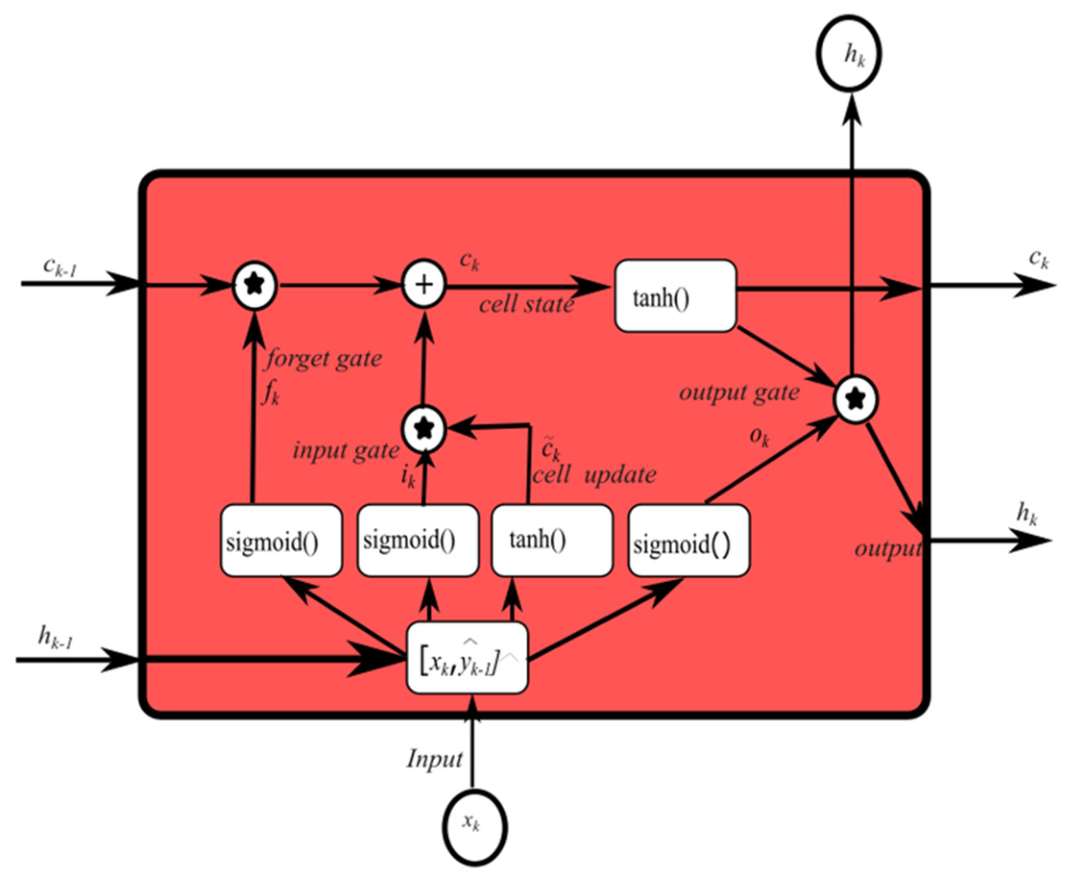
LSTMs address this challenge by introducing a memory cell capable of storing information over long periods, as well as gating mechanisms that regulate the flow of information. As shown in Figure 2, an LSTM unit consists of four essential components: the cell state, hidden state, input vector, and a set of nonlinear activation functions, typically the sigmoid and hyperbolic tangent (tanh) functions.
C k 1 represents the previous cell state, C k is the current cell state, C ~ k is the cell update, x[k] is the input data. h k 1 represents the previous hidden state, h k is the current hidden state. σ is the sigmoid function, f k is the forget gate, i k is the input gate, o k is the output gate. w i , w f , w o , w c represent weights applied for the input gate, forget gate, output gate and cell state respectively. b i , b f , b o , b c represent biases applied for the input gate, forget gate, output gate and cell state respectively.
LSTM equations for the gates are as follows:
i k =   σ ( w i h k 1 ,   x k + b i )
f k = σ ( w f h k 1 ,   x k + b f
o k = σ ( w o h k 1 ,   x k + b o
LSTM equations for the cell state, candidate cell state and final output are as follows:
C ~ k =   t a n h ( w c h k 1 ,   x k + b c )
C k = f t C k 1 + i k C ~ k
h k = o t t a n h ( C k )

LSTM Model Development

This section describes the process that was used to develop the LSTM model.
  • Data Acquisition and Preprocessing
Environmental and atmospheric datasets, which often contain missing values, irregular time steps, and noise, were first collected from relevant monitoring networks. Preprocessing included handling missing data, normalizing variables, and performing time-series smoothing where necessary. Data were then segmented into training, validation, and testing sets to ensure robust evaluation.
  • Feature Engineering
Relevant predictors such as temperature, humidity, wind speed, and historical pollutant concentrations were selected. Lag features and rolling statistics were introduced to capture temporal dependencies and enhance model performance.
  • Model Architecture Design
The LSTM model was constructed using one or more stacked LSTM layers, followed by dense layers for regression output. Hyperparameters such as the number of units, learning rate, batch size, and sequence length were optimized through experimentation.
  • Model Training
The model was trained using a suitable optimizer (e.g., Adam) and a loss function such as Mean Squared Error (MSE). Early stopping and dropout regularization were implemented to prevent overfitting.
  • Model Evaluation
Performance was assessed using metrics such as Root Mean Squared Error (RMSE).
  • Model Deployment and Interpretation
After training, the best model was deployed for forecasting. Feature importance and temporal sensitivity analysis were conducted to assess model interpretability. More details on the model deployment can be found in [24,25,26,27].
Optimizing feature engineering for air quality prediction requires transforming raw environmental observations into informative inputs that effectively represent the complex and non-linear behaviour of atmospheric pollutants. Important optimization strategies include incorporating temporal dependencies, modelling interactions among pollutants, and applying automated feature selection techniques. Because air quality is strongly influenced by recent atmospheric conditions, refining these features enables predictive models to better identify both short-term pollution episodes and long-term variation patterns.
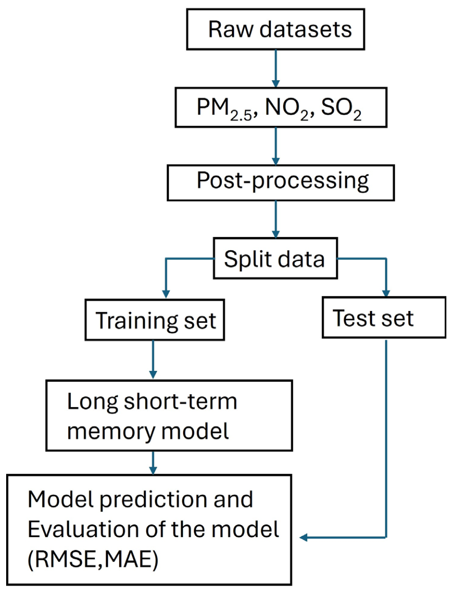
All raw data acquired from the open-access database were integrated into a unified dataset and subjected to preprocessing procedures, including the identification and treatment of missing values and the encoding of categorical variables. The processed dataset was subsequently divided into training and testing subsets to facilitate model development and evaluation. A Long Short-Term Memory (LSTM) neural network was then implemented to predict PM2.5, SO2, and NO2 concentrations. The overall methodological framework employed for pollutant prediction is illustrated in Figure 3. Model performance was assessed by comparing observed and predicted pollutant concentrations using the Root Mean Square Error (RMSE) and Mean Absolute Error (MAE) metrics. To optimize predictive performance, key hyperparameters, including the learning rate, number of training epochs, and batch size, were systematically adjusted.
The LSTM model was trained on a comprehensive dataset spanning 1 July 2018 to 25 November 2025 and forecasted for 26 November 2025. This period provides a rich record of atmospheric parameters and pollutant concentrations necessary for accurate air quality forecasting. By leveraging several years of historical observations, the model can capture long-term trends, seasonal variability, and complex temporal dependencies in the data. Such an extended and diverse training dataset enhances the model’s ability to generalize effectively, resulting in more reliable predictions for PM2.5, SO2, NO2, and the Air Quality Index (AQI). Table 1 summarizes the architecture and hyperparameter configuration of the LSTM model used for pollutant and air quality prediction. The model consists of LSTM and dense layers designed to capture temporal dependencies in the pollutant concentration data. Key training parameters, including the input shape, optimizer, learning rate, batch size, and number of epochs, were selected through experimental tuning to achieve optimal predictive performance. These settings enabled the model to effectively learn the underlying patterns in the time-series data and improve prediction accuracy.

4. Results and Discussion

4.1. Spatial Distribution Maps for NO2, SO2 and PM2.5

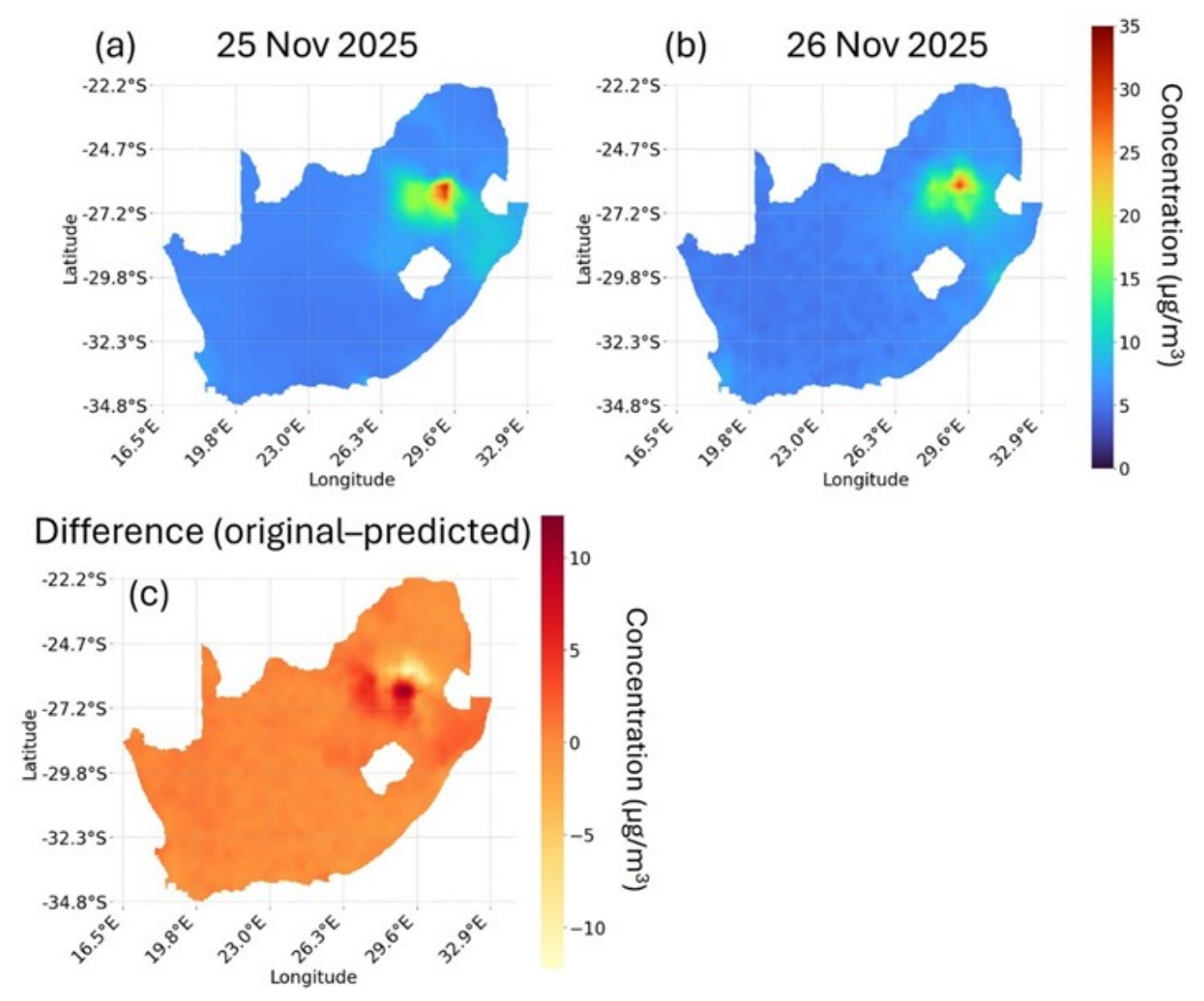
The NO2 observations over South Africa for 25 and 26 November 2025 reveal a consistent spatial pattern dominated by a prominent pollution hotspot in the north-eastern interior, corresponding to the Mpumalanga Highveld and parts of Gauteng. Figure 4a,b show that this region exhibits the highest NO2 concentrations, exceeding 25–30 μg/m3 on both days, reflecting persistent emissions from coal-fired power stations, industrial operations, and dense urban activity. In contrast, the rest of the country displays low background levels, typically below 5 μg/m3, particularly over the western and southern regions where major anthropogenic sources are limited. Although the overall pattern remains stable between the two days, subtle variations in magnitude and spatial extent are evident, likely influenced by meteorological conditions such as wind transport and boundary-layer dynamics. Figure 4c, which presents the difference between the original and machine-learning-predicted fields, indicates that the model reproduces the spatial distribution reasonably well across most regions, with residuals close to zero over large parts of the country. However, the largest discrepancies occur within the Highveld hotspot, where the model tends to underestimate peak concentrations in some areas while slightly overestimating nearby regions. These mixed residuals reflect the model’s challenge in capturing sharp emission gradients and highly localized sources. Overall, the figure highlights both the persistent nature of NO2 pollution in South Africa’s industrial heartland and the strengths and limitations of the predictive model in representing these patterns.
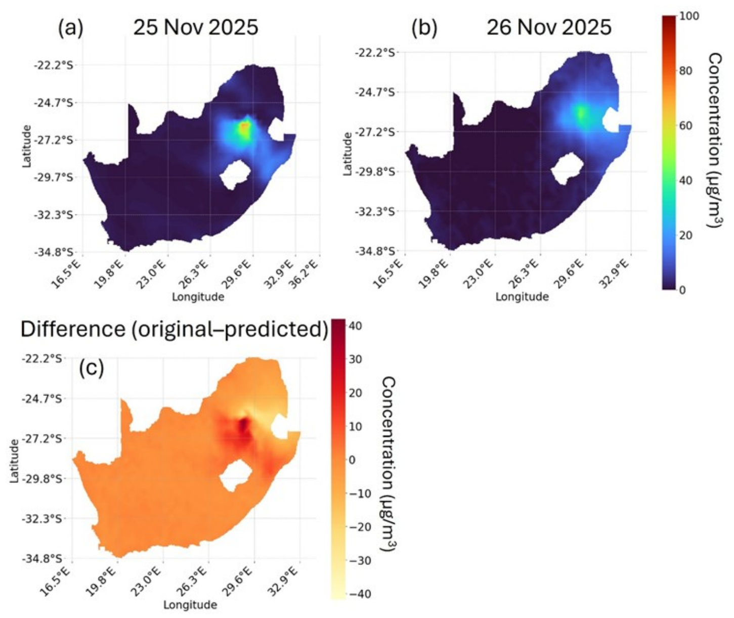
Figure 5 highlights a clear and persistent SO2 hotspot, consistent with known industrial emission regions, and they demonstrate both the strength and limitations of the prediction model in capturing sharp spatial gradients. Figure 5a,b show that SO2 concentrations are strongly concentrated in the north-eastern interior, particularly around the Mpumalanga Highveld, a region dominated by coal-fired power stations and heavy industry. On 25 November 2025, the hotspot displays elevated SO2 values exceeding 60–80 μg/m3, indicating intense emissions localized around major industrial facilities. On 26 November 2025, the hotspot persists, with slightly higher concentration levels and broader spatial spread, suggesting either increased emissions or meteorological conditions that favoured pollutant accumulation, such as lower boundary-layer height or weaker winds. Outside of this core region, SO2 levels across South Africa remain very low, typically close to 0–10 μg/m3, reflecting limited industrial sources in the western, northern, and southern parts of the country. Figure 5c presents the difference between the original and predicted SO2 fields, providing insight into model performance. Residuals are relatively small across most of the country, indicating that the model captures the broad spatial distribution well. However, large positive and negative differences appear within and around the SO2 hotspot. In some localized areas the model underestimates peak concentrations (positive residuals up to ~40 μg/m3), while in nearby areas it overestimates concentrations (negative residuals down to −40 μg/m3). These alternating residuals point to the difficulty of accurately predicting SO2 in regions with steep emission gradients, rapidly changing plume structures, or strong point-source influences typical of the Highveld power plant complex. Overall, the results confirm that the Mpumalanga Highveld remains the dominant SO2 emission region in South Africa and underscore the challenges for predictive models in resolving sharp, localised emission features, even when they perform well on regional spatial patterns.
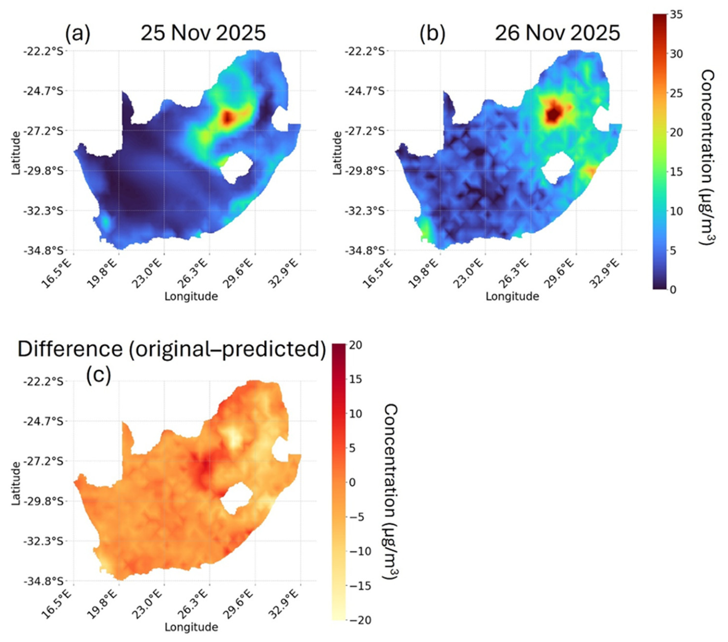
Figure 6a,b both show a prominent PM2.5 hotspot located in the north-eastern interior, corresponding to the Mpumalanga Highveld. On 25 November 2025, concentrations exceed 25–30 µg/m3 in the hotspot area, with a distinct plume extending eastward and south eastward. By 26 November 2025, the hotspot becomes even more pronounced; concentrations increase and the polluted region expands spatially. The broader spread and slightly higher values on the 26th of November may reflect changes in meteorological conditions—such as reduced dispersion, shifts in wind direction, or a shallower planetary boundary layer—allowing particulate matter to accumulate more readily. Across the rest of the country, PM2.5 concentrations remain low, typically below 5–10 µg/m3, consistent with lower emission activity outside the Highveld and major metropolitan areas. Figure 6c presents the difference between the original and predicted PM2.5 fields, offering insight into model performance. The residuals are generally small across most of the country, indicating that the model captures the broad spatial pattern reasonably well. However, the largest discrepancies occur around the Highveld hotspot, where some locations show positive residuals (original > predicted), meaning the model underestimates peak concentrations. Other nearby areas show negative residuals, indicating overestimation. These alternating patterns of under- and over-prediction are typical in regions of strong point-source emissions and steep pollutant gradients, where minor shifts in plume structure or spatial variability can lead to noticeable deviations. Overall, the results confirm that PM2.5 pollution in South Africa during this period is heavily concentrated in the industrialized Highveld, while most other regions experience relatively clean conditions. The prediction model performs well at reproducing national spatial patterns but faces challenges in areas where emissions are highly localized and atmospheric processes increase variability.

4.2. Spatial Distribution Maps for AQI

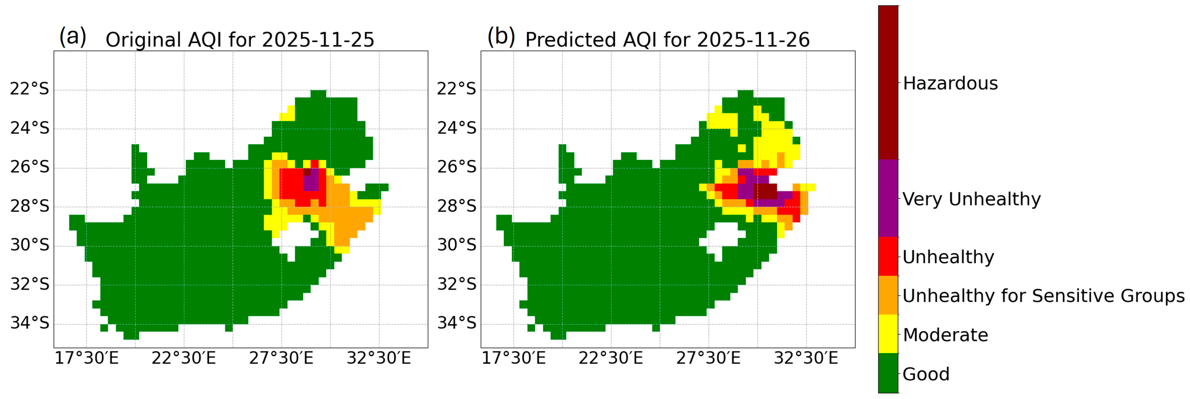
Figure 7 presents the Air Quality Index (AQI) classification over South Africa for 25 November 2025 (original data) and 26 November 2025 (predicted data), highlighting how pollutant levels translate into potential health impacts across different regions. The results clearly show strong spatial contrasts, with most of the country experiencing good air quality while a concentrated region in the interior exhibits degraded conditions. In Figure 7a, the majority of South Africa is categorized as “Good” (green), indicating low pollution levels and minimal health risk. However, a pronounced hotspot appears in the north-eastern interior, centered over the Mpumalanga Highveld and extending slightly into Gauteng. This region contains the country’s largest cluster of coal-fired power plants and industrial activities, which strongly influence local air quality. Within this hotspot, AQI values escalate from “Moderate” (yellow) to “Unhealthy for Sensitive Groups” (orange) and “Unhealthy” (red). The core of the hotspot even reaches “Very Unhealthy” (purple), suggesting a high level of pollution capable of affecting the entire population, not only vulnerable groups. This pattern aligns with elevated pollutant concentrations observed for SO2, NO2, and PM2.5 in previous analyses. The predicted AQI for Figure 7b shows a very similar spatial structure, indicating that the machine-learning model effectively reproduces the hotspot’s form and intensity. The Highveld region again exhibits widespread zones classified as Unhealthy, and pockets of Very Unhealthy, with some peripheral expansion into areas previously showing lower AQI categories. This slight broadening may reflect day-to-day changes in meteorological conditions that favour pollutant accumulation or transport, such as shifts in wind direction or lower atmospheric mixing. The good agreement between the original and predicted spatial patterns demonstrates the model’s capacity to capture both the geographical extent and severity of pollution levels. Overall, the results highlight that while most regions in South Africa maintain good air quality, the Mpumalanga Highveld remains a persistent and severe air-pollution hotspot, with AQI levels regularly reaching thresholds associated with significant public-health risks. The similarity between the observed and predicted distributions further confirms the model’s strong performance in forecasting air-quality categories across the country.

4.3. Model Performance and Error Analysis

The error analysis results, summarized in Table 2, provide a quantitative assessment of the machine-learning model’s ability to reproduce the spatial patterns of SO2, NO2, PM2.5, and AQI over South Africa. Overall, the very small error values across all variables indicate strong model performance and good agreement between the original satellite-derived fields and the predicted outputs. The RMSE (Root Mean Square Error) values for all pollutants are extremely low, with PM2.5 showing the smallest error (0.0021) and AQI the largest (0.0204). These magnitudes reflect that the model captures pollutant concentrations with high precision, particularly for PM2.5, where the model’s predictions closely follow the observed gradients. Similarly, the MSE (Mean Square Error) values are near zero for all variables, again demonstrating minimal deviation between predicted and original values. Among the pollutants, SO2 and NO2 exhibit slightly higher RMSE values relative to PM2.5, which is expected given the sharp spatial gradients and highly localized emission sources associated with these gases. Their plumes often vary abruptly over small distances, making them more challenging for models to predict perfectly. The comparatively larger RMSE for AQI (0.02039) is also reasonable, as AQI integrates multiple pollutants into categorical air-quality levels. Any small deviation in predicted pollutant concentrations can shift cells from one AQI category to another, increasing the apparent error even if the underlying concentration data remain highly accurate. Despite this, the AQI error values remain low, reflecting strong model skill in reproducing health-based air-quality classifications. Overall, the results confirm that the predictive model performs very well, with extremely small RMSE and MSE values across all pollutants and AQI. The model effectively captures both the magnitude and spatial distribution of air-pollution patterns, and the modest deviations observed for gases with steep gradients (SO2 and NO2) are expected and do not detract from the model’s overall reliability.

5. Conclusions

The analysis of satellite-derived and LSTM-predicted air-quality fields for South Africa demonstrates that the model effectively captures the spatial distribution and intensity of key pollutants, including SO2, NO2, PM2.5, and the resulting AQI classifications. Across all variables, the results consistently highlight the Mpumalanga Highveld as the dominant pollution hotspot, driven by concentrated coal-fired power generation and industrial activities. This region repeatedly exhibits elevated pollutant levels and degraded air quality, while most other parts of the country maintain comparatively clean conditions.
The strong agreement between the original and predicted fields—visible in the spatial maps and confirmed by the very low RMSE and MSE values—indicates that the model reliably reproduces both the magnitude and spatial variability of air-pollution patterns. Although minor discrepancies occur in areas with sharp emission gradients and highly localized plumes, these differences are expected and do not significantly affect the overall performance. The model’s ability to replicate AQI categories further reinforces its robustness, even when translating pollutant concentrations into health-based classifications.
Overall, the findings demonstrate that the LSTM provides an accurate and reliable tool for predicting air-quality conditions over South Africa. Its strong performance suggests that it can support operational air-quality forecasting, environmental monitoring, and policy-relevant assessments, particularly in regions where pollutant exposure poses persistent health risks.

Author Contributions

Conceptualization, L.S. and M.S., methodology, L.S. and M.S.; formal analysis, L.S., M.S. and N.M.; investigation, L.S.; writing—original draft preparation, L.S.; writing—review and editing, M.S., M.M., H.H. and N.M. All authors have read and agreed to the published version of the manuscript.

Funding

This research received no external funding.

Institutional Review Board Statement

Not applicable.

Informed Consent Statement

Not applicable.

Data Availability Statement

TROPOMI data is obtained on the Google Earth Engine platform.

Acknowledgments

The authors thank the European Space Agency (ESA) and its collaborators for providing the Sentinel-5P/TROPOMI data used in this study.

Conflicts of Interest

The authors declare no conflicts of interest.

References

  1. Samal, K.K.R.; Panda, A.K.; Babu, K.S.; Das, S.K. An improved pollution forecasting model with meteorological impact using multiple imputation and fine-tuning approach. Sustain. Cities Soc. 2021, 70, 102923. [Google Scholar] [CrossRef]
  2. Bekkar, A.; Hssina, B.; Douzi, S.; Douzi, K. Air-pollution prediction in smart city, deep learning approach. J. Big Data 2021, 8, 161. [Google Scholar] [CrossRef] [PubMed]
  3. Mao, W.; Jiao, L.; Wang, W.; Wang, J.; Tong, X.; Zhao, S. A hybrid integrated deep learning model for predicting various air pollutants. GISci. Remote Sens. 2021, 58, 1395–1412. [Google Scholar] [CrossRef]
  4. Chen, G.; Chen, S.; Li, D.; Chen, C. A hybrid deep learning air pollution prediction approach based on neighborhood selection and spatio-temporal attention. Sci. Rep. 2025, 15, 3685. [Google Scholar] [CrossRef] [PubMed]
  5. Li, D.; Liu, J.; Zhao, Y. Prediction of multi-site PM2.5 concentrations in Beijing using CNN-BiLSTM with CBAM. Atmosphere 2022, 13, 1719. [Google Scholar] [CrossRef]
  6. Qin, D.; Yu, J.; Zou, G.; Yong, R.; Zhao, Q.; Zhang, B. A novel combined prediction scheme based on CNN and LSTM for urban PM2.5 concentration. IEEE Access 2019, 7, 20050–20059. [Google Scholar] [CrossRef]
  7. Necula, S.-C.; Hauer, I.; Fotache, D.; Hurbean, L. Advanced hybrid models for air pollution forecasting: Combining SARIMA and BiLSTM architectures. Electronics 2025, 14, 549. [Google Scholar] [CrossRef]
  8. Cabaneros, S.M.; Calautit, J.K.; Hughes, B.R. A review of artificial neural network models for ambient air pollution prediction. Environ. Model. Softw. 2019, 119, 285–304. [Google Scholar] [CrossRef]
  9. Jiang, P.; Dong, Q.; Li, P. A novel hybrid strategy for PM2.5 concentration analysis and prediction. J. Environ. Manag. 2017, 196, 443–457. [Google Scholar] [CrossRef] [PubMed]
  10. Salman, A.G.; Heryadi, Y.; Abdurahman, E.; Suparta, W. Single-layer and multi-layer long short-term memory (LSTM) model with intermediate variables for weather forecasting. Procedia Comput. Sci. 2018, 135, 89–98. [Google Scholar] [CrossRef]
  11. Wang, S.; McGibbon, J.; Zhang, Y. Predicting high-resolution air quality using machine learning: Integration of large eddy simulation and urban morphology data. Environ. Pollut. 2024, 344, 123371. [Google Scholar] [CrossRef] [PubMed]
  12. Ngamlana, N.B.; Malherbe, W.; Gericke, G.; Coetzer, R.L.J. The effect of coal-fired power plants on ambient air quality in Mpumalanga Province, South Africa, 2014–2018. Int. J. Environ. Health Res. 2025, 35, 220–232. [Google Scholar] [CrossRef] [PubMed]
  13. Williams, C.R.; Leaner, J.J.; Nel, J.M.; Somerset, V.S. Mercury concentrations in water resources potentially impacted by coal-fired power stations and artisanal gold mining in Mpumalanga, South Africa. J. Environ. Sci. Health A 2010, 45, 1363–1373. [Google Scholar] [CrossRef] [PubMed]
  14. Laisani, J.; Jegede, A.O. Impacts of coal mining in Witbank, Mpumalanga Province of South Africa: An eco-legal perspective. J. Rev. Glob. Econ. 2019, 8, 1586–1597. [Google Scholar] [CrossRef]
  15. Balashov, N.V.; Thompson, A.M.; Piketh, S.J.; Langerman, K.E. Surface ozone variability and trends over the South African Highveld from 1990 to 2007. J. Geophys. Res. Atmos. 2014, 119, 4323–4342. [Google Scholar] [CrossRef]
  16. Magagula, M.; Atangana, E.; Oberholster, P. Assessment of the impact of coal mining on water resources in Middelburg, Mpumalanga Province, South Africa using different water quality indices. Hydrology 2024, 11, 113. [Google Scholar] [CrossRef]
  17. Laakso, L.; Vakkari, V.; Virkkula, A.; Laakso, H.; Backman, J.; Kulmala, M.; Beukes, J.P.; Van Zyl, P.G.; Tiitta, P.; Josipovic, M.; et al. South African EUCAARI measurements: Seasonal variation of trace gases and aerosol optical properties. Atmos. Chem. Phys. 2012, 12, 1847–1864. [Google Scholar] [CrossRef]
  18. Theys, N.; Hedelt, P.; De Smedt, I.; Lerot, C.; Yu, H.; Vlietinck, J.; Pedergnana, M.; Arellano, S.; Galle, B.; Fernandez, D.; et al. Global monitoring of volcanic SO2 degassing with unprecedented resolution from TROPOMI onboard Sentinel-5 Precursor. Sci. Rep. 2019, 9, 2643. [Google Scholar] [CrossRef] [PubMed]
  19. Tilstra, L.G.; de Graaf, M.; Wang, P.; Stammes, P. In-orbit Earth reflectance validation of TROPOMI onboard the Sentinel-5 Precursor satellite. Atmos. Meas. Tech. 2020, 13, 4479–4497. [Google Scholar] [CrossRef]
  20. Verhoelst, T.; Compernolle, S.; Pinardi, G.; Lambert, J.C.; Eskes, H.J.; Eichmann, K.U.; Fjæraa, A.M.; Granville, J.; Niemeijer, S.; Cede, A.; et al. Ground-based validation of the Copernicus Sentinel-5P TROPOMI NO2 measurements with the NDACC ZSL-DOAS, MAX-DOAS and Pandonia global networks. Atmos. Meas. Tech. 2021, 14, 481–510. [Google Scholar] [CrossRef]
  21. Prakash, S.; Jalal, A.S.; Pathak, P. Forecasting COVID-19 pandemic using Prophet, LSTM, hybrid GRU-LSTM, CNN-LSTM, Bi-LSTM and stacked-LSTM for India. In Proceedings of the 6th International Conference on Information Systems and Computer Networks (ISCON), Mathura, India, 3–4 March 2023; IEEE: Piscataway, NJ, USA, 2023; pp. 1–6. [Google Scholar] [CrossRef]
  22. Luo, J.; Gong, Y. Air pollutant prediction based on ARIMAWOA-LSTM model. Atmos. Pollut. Res. 2023, 14, 101761. [Google Scholar] [CrossRef]
  23. Hamayel, M.J.; Owda, A.Y. A novel cryptocurrency price prediction model using GRU, LSTM and Bi-LSTM machine learning algorithms. AI 2021, 2, 477–496. [Google Scholar] [CrossRef]
  24. Zheng, Y.; Liu, F.; Hsieh, H.P. U-Air: When Urban Air Quality Inference Meets Big Data. In Proceedings of the 21th ACM SIGKDD International Conference on Knowledge Discovery and Data Mining; ACM: Sydney, Australia, 2015; pp. 1436–1444. [Google Scholar]
  25. Li, X.; Peng, L.; Hu, Y.; Shao, J.; Chi, T. Deep Learning Architecture for Air Quality Predictions. Environ. Sci. Pollut. Res. 2016, 23, 22408–22417. [Google Scholar] [CrossRef] [PubMed]
  26. Du, Y.; Xu, Y.; Chu, X.; Guo, J.; Wang, Y. Air Quality Forecasting Using a Hybrid Deep Learning Model. Atmos. Environ. 2018, 181, 244–255. [Google Scholar]
  27. Kumar, P.; Morawska, L.; Martani, C.; Biskos, G.; Neophytou, M.; Di Sabatino, S.; Bell, M.; Norford, L.; Britter, R. Forecasting Air Quality Using Deep Recurrent Neural Networks. Sci. Total Environ. 2019, 650, 1506–1515. [Google Scholar]
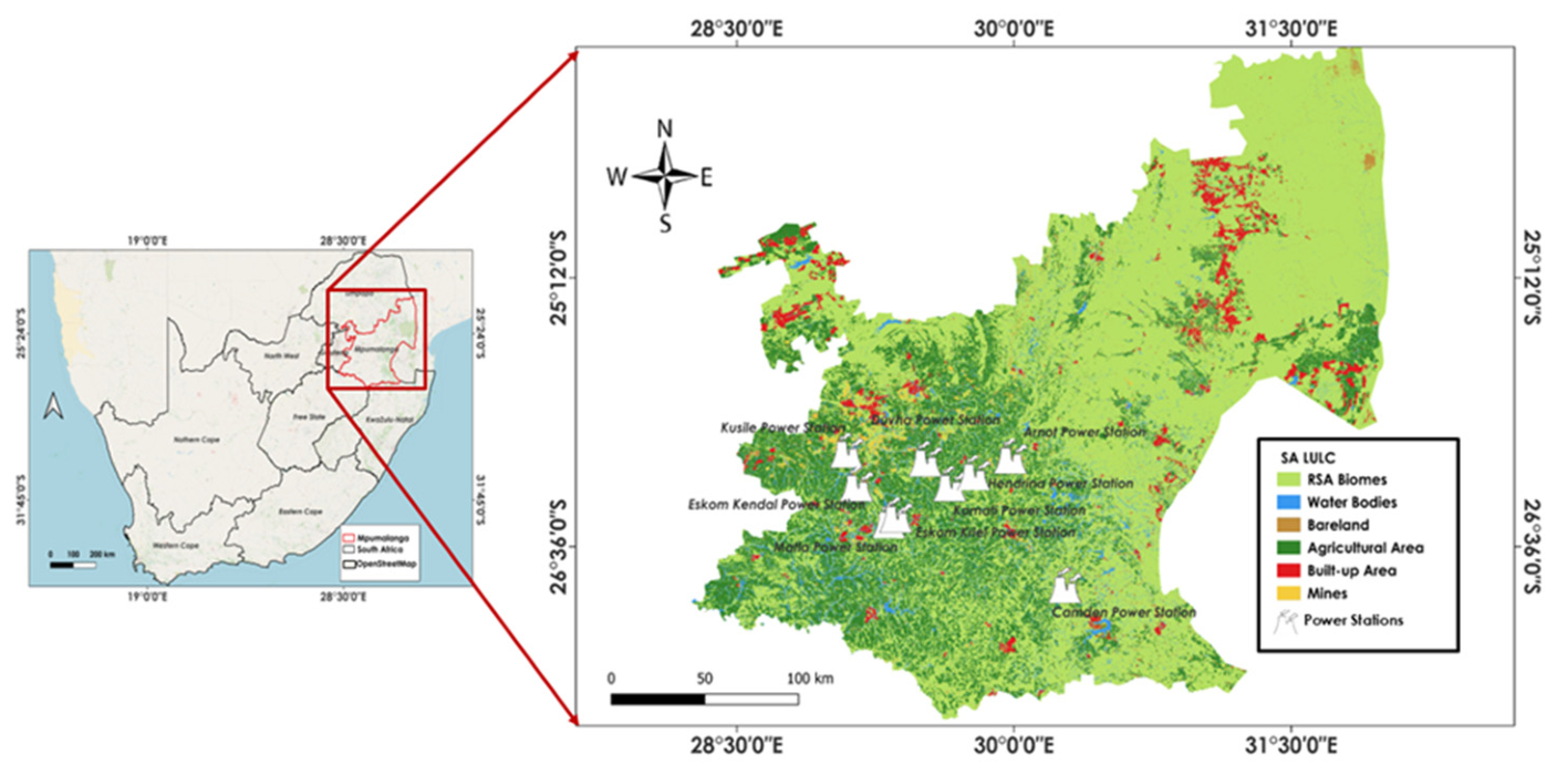
Figure 1. Map of the study area highlighting South Africa and the Mpumalanga Province, indicating major industrial emission sources alongside key land-cover classes such as built up, agricultural, mining, and natural vegetation.
Atmosphere 17 00610 g001
Figure 2. The structure of the long short-term memory (LSTM) unit.
Atmosphere 17 00610 g002
Figure 3. Workflow for predicting pollutant concentration and the air quality index (AQI) using the LSTM model.
Atmosphere 17 00610 g003
Figure 4. Spatial distribution of NO2 concentrations over South Africa for (a) 25 November 2025 and (b) 26 November 2025, showing a persistent hotspot over the Mpumalanga Highveld associated with major industrial and power-generation activities. (c) The difference between the original satellite-derived NO2 fields and the machine-learning-predicted values.
Atmosphere 17 00610 g004
Figure 5. Spatial distribution of SO2 concentrations over South Africa for (a) 25 November 2025 and (b) 26 November 2025. (c) The difference between the original satellite-derived SO2 fields and the machine-learning predictions.
Atmosphere 17 00610 g005
Figure 6. Spatial distribution of PM2.5 concentrations over South Africa for (a) 25 November 2025 and (b) 26 November 2025. (c) The difference between the original PM2.5 fields and the machine-learning predictions.
Atmosphere 17 00610 g006
Figure 7. Air Quality Index (AQI) classification over South Africa for (a) the original AQI on 25 November 2025 and (b) the machine-learning-predicted AQI for 26 November 2025.
Atmosphere 17 00610 g007
Table 1. Architecture and Hyperparameter Configuration of the LSTM Model.
ComponentConfiguration
Model TypeLong Short-Term Memory (LSTM)
Input Shape(3615, 1)
Input FeaturesPM2.5, SO2, NO2, AQI
LSTM Layer 164 units, return sequences = True
Dropout Layer 10.2
LSTM Layer 232 units, return sequences = False
Dropout Layer 20.2
Dense Layer16 units, ReLU activation
Output Layer1 unit, Linear activation
Loss FunctionMean Squared Error (MSE)
OptimizerAdam
Learning Rate0.001
Batch Size32
Epochs50
Validation Split30%
Evaluation MetricsRMSE, MSE
Table 2. Root Mean Square Error (RMSE) and Mean Square Error (MSE) values for SO2, NO2, PM2.5, and AQI, illustrating the overall prediction accuracy of the LSTM model.
VariableRMSEMSE
SO20.016167647970070.0002628326944634
NO20.011816249553780.0001395414387
PM2.50.00205673757491262174.230169452057453 × 10−6
AQI0.0203900.000416
Disclaimer/Publisher’s Note: The statements, opinions and data contained in all publications are solely those of the individual author(s) and contributor(s) and not of MDPI and/or the editor(s). MDPI and/or the editor(s) disclaim responsibility for any injury to people or property resulting from any ideas, methods, instructions or products referred to in the content.