Topographic and Potential-Radiation Relationships with Ground-Surface Thermal Response During the Thawing Period in Maritime Antarctica

Abstract

Ground-surface temperature (GST) in maritime Antarctic ice-free areas is influenced by atmospheric forcing, snow cover, surface energy and topography. Previous PERMATHERMAL studies in Livingston and Deception Islands have shown changes in air and ground-surface thermal regimes, with fewer cold conditions, greater thawing influence and strong snow-cover modulation. However, the interval in which GST responds effectively to radiative and topographic forcing remains poorly explored. We characterize the station- and season-specific timing of the thermally effective GST thawing period and evaluate topographic and modeled potential controls on its thermal intensity and cumulative effect around the Spanish Antarctic Station Juan Carlos I, Hurd Peninsula, Livingston Island. Onset and end were objectively delimited by using three consecutive days with daily mean GST > 0.5 °C and daily thermal amplitude > 1.0 °C. Hourly GST records from six PERMATHERMAL stations were combined with potential radiation, potential insolation and topographic variables derived from a high-resolution UAV-based DEM. Accumulated thawing degree days were strongly influenced by period duration. Mean thermal intensity was primarily associated with elevation, while mean modeled potential radiation provided additional explanatory power only when combined with elevation. This UAV–GIS–GST approach provides a simple framework for assessing local surface–atmosphere coupling in remote Antarctic ice-free areas.

1. Introduction

Ice-free areas of maritime Antarctica are among the most climatically sensitive terrestrial environments in the North-western Antarctic Peninsula region, where recent atmospheric variability has affected snow cover, ground thermal regimes, active-layer dynamics and the stability of marginal permafrost conditions [1,2,3,4,5]. In these environments, ground-surface temperature (GST) is a key variable linking atmospheric forcing, snow cover and the shallow subsurface, because it controls the amount of energy transferred to the ground and influences seasonal thaw, geomorphological activity, hydrological processes and ecological conditions in ice-free terrain [6,7,8,9,10,11]. Understanding when and how GST becomes coupled to atmospheric and radiative forcing is therefore essential for interpreting local differences in frozen-ground conditions in Antarctic environments located close to the climatic limit of permafrost occurrence [1,2,4,5,12].

The ground thermal regime is strongly influenced by incoming solar radiation and by local topographic factors such as elevation, slope and aspect, which determine the amount and timing of energy potentially available at the surface [6,13,14,15]. However, the relationship between modeled potential solar radiation and GST is not direct, particularly in environments where snow cover, soil moisture and ground ice strongly modulate the surface energy balance [6,7,8,16]. While the surface is snow-covered, part of the available energy may be consumed by snowmelt, metamorphism or changes in snowpack properties rather than by warming the ground surface [6,16]. Similarly, once snow has disappeared, the ground may remain close to 0 °C while energy is consumed by phase changes associated with ice-rich or water-saturated near-surface materials, producing a zero-curtain-like thermal behavior [17]. Consequently, the period during which modeled potential radiation can be expected to produce a measurable increase in GST does not necessarily coincide with the full summer season or even with the entire physically snow-free period.

This distinction is particularly relevant in the South Shetland Islands, where snow cover is spatially heterogeneous and strongly affected by wind redistribution, local topography and exposure [18,19,20,21,22,23]. Livingston Island, and especially Hurd Peninsula around the Spanish Antarctic Station “Juan Carlos I” (hereafter SAS-JCI), lies close to the lower limit of regional permafrost distribution, in an environment characterized by sporadic to discontinuous permafrost conditions where small differences in elevation, snow persistence, exposure or soil conditions can determine whether perennially frozen ground is present or absent [1,2,13,21]. In this setting, nearby sites can show contrasting GST regimes because the timing of snow disappearance, the duration of zero-curtain conditions and the length of the effective positive-temperature period differ over short distances [18,19,21,22,23]. These local contrasts are important not only for interpreting active-layer development and shallow permafrost persistence, but also for understanding how surface–atmosphere coupling varies within short spatial gradients in maritime Antarctic environments.

Previous studies of the PERMATHERMAL network have documented complementary aspects of the atmosphere–ground thermal system in Livingston and Deception Islands. Long-term GST analyses have shown increasing thawing influence, changes in daily thermal regimes and a progressive shift towards warmer ground-surface conditions between 2007 and 2021 [22]. A subsequent phase-based GST analysis showed that the annual ground-surface thermal cycle includes cooling, attenuation, insulation, melting and zero-curtain phases, and that snow cover strongly modulates the timing and expression of the ground thermal regime [23]. In parallel, recent air-temperature analyses indicate that warming is expressed not only as increasing mean annual air temperature, but also as a reorganization of the annual thermal calendar, with fewer cold days, more thaw-related conditions and less negative annual degree–day balance [24]. Together, these studies show that the thermal state of the ground surface cannot be understood from air temperature, snow cover or local topography alone, but requires attention to the timing of surface–atmosphere coupling during the thawing season.

More complex numerical models have been applied to simulate permafrost temperature evolution and active-layer thickness in Antarctic Peninsula environments, but these approaches require detailed meteorological forcing, snow parameterization and soil thermal properties that are not always available at the local scale in remote areas [14,15]. There is therefore room for simpler empirical approaches that combine field GST observations with high-resolution topographic and radiative variables derived from UAV-photogrammetric surveys and GIS-based modeling. Such approaches do not replace energy balance or permafrost models, but they can help identify which part of the surface thermal signal is organized by topographic and radiative forcing once snowmelt and phase-change-dominated conditions have ended.

The PERMATHERMAL monitoring stations around the SAS-JCI (Figure 1) provide a suitable framework for this type of analysis because they combine GST observations along a short altitudinal transect with high-resolution UAV-derived topographic information (Figure 2). The UAV-derived DEM also makes it possible to generate spatially distributed maps of modeled potential radiation and potential insolation, allowing point GST observations to be interpreted within a broader terrain-controlled radiative field. Following previous criteria that identify the transition from the zero-curtain period to the warm phase as the onset of the ground-surface thawing period, we focus on the interval in which GST shows a sustained positive-temperature response and can therefore be compared with modeled potential radiation and local topographic variables [23,25,26].

The aim of this study is to characterize the station- and season-specific timing of the thermally effective ground-surface thawing period and to evaluate whether UAV-derived topographic variables and modeled potential solar radiation estimates can explain its thermal intensity and cumulative thermal effect in a maritime Antarctic environment. Specifically, we: (i) identify the thermally effective thawing period from daily GST records at PERMATHERMAL stations around the SAS-JCI; (ii) quantify its timing, duration, mean thermal intensity and accumulated thawing degree days; (iii) generate spatially distributed topographic, potential-radiation and potential-insolation products from a high-resolution UAV-derived digital elevation model; and (iv) assess the relationships of thermal intensity and thermal accumulation with local topographic and radiative variables using simple empirical models, while using timing variables to contextualize the cumulative indices.

2. Study Area, Data and Methods

2.1. Study Area and Monitoring Stations

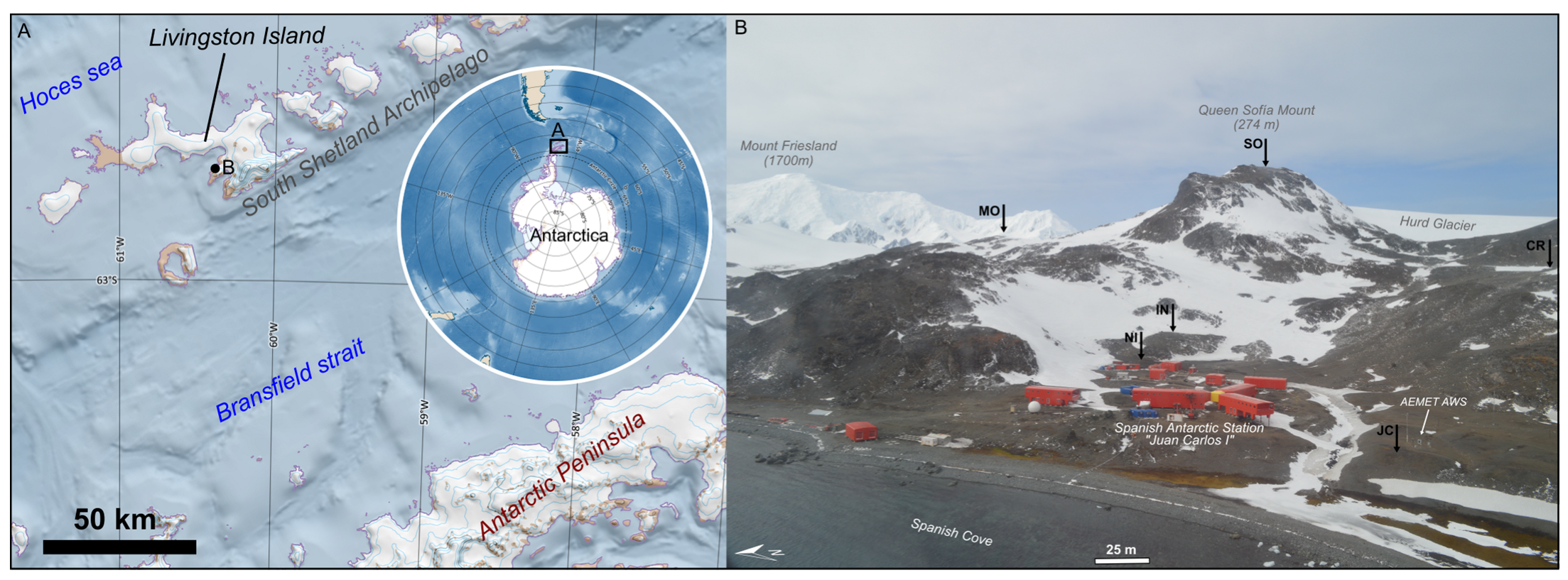
The study was carried out in the surroundings of the SAS-JCI, on Hurd Peninsula, Livingston Island, South Shetland Islands, maritime Antarctica (Figure 1). Six PERMATHERMAL monitoring stations were used in this study: Juan Carlos I (JC), Nuevo Incinerador (NI), Incinerador (IN), Collado Ramos (CR), Morrena (MO) and Sofía (SO) (

Table 1. Location and topographic characteristics of the PERMATHERMAL monitoring stations used in this study.

Station	Name	Latitude	Longitude	Elevation (m a.s.l.)	Slope (°)	Aspect (°)	Pseudo-Albedo	Geomorphological Setting	Wind Exposure
JC	Juan Carlos I	62°39′48.815″ S	60°23′26.484″ W	10.8	2.0	158.6	0.55	Raised beaches	Low
NI	Nuevo Incinerador	62°39′50.744″ S	60°23′09.061″ W	18.5	3.9	279.3	0.47	Slope foot	Very low
IN	Incinerador	62°39′52.980″ S	60°23′08.079″ W	33.4	7.0	267.1	0.52	Rock step in slope	Low
CR	Collado Ramos	62°40′03.063″ S	60°23′31.504″ W	115.9	4.3	59.2	0.59	Wide, flat interfluve	High
MO	Morrena	62°40′01.671″ S	60°22′31.430″ W	149.3	6.3	135.9	0.44	Lateral moraine	High
SO	Sofía	62°40′15.657″ S	60°22′46.468″ W	274.1	2.6	205.0	0.39	Slope top near summit	Very high

). These stations are distributed along a short altitudinal gradient across the ice-free terrain around the base, from the coastal sector of South Bay to the upper slopes of Mount Reina Sofía, between approximately 10 and 274 m a.s.l. (Table 1).

The area has a cold maritime Antarctic climate, with mean annual air temperature close to −2 to −1 °C at sea level and progressively lower values with altitude [20,27,28,29]. Previous observations indicate that MAAT may decrease to around −4 °C at Mount Reina Sofía, the highest sector included in this study [23,30]. Annual precipitation at sea level is approximately 500 mm and occurs mainly as snow, although liquid precipitation may occur during summer at low elevations [23,31]. The area is also characterized by frequent winds and big local differences in exposure, which contribute to heterogeneous snow redistribution and short-distance variability in surface conditions [20,23,31].

The stations are located on representative ice-free surfaces around the base, generally in wind-exposed positions where prolonged insulating snow accumulation is limited [6,32]. However, local differences in exposure and snow redistribution occur between sites, particularly near slope bases and areas affected by drifting snow [21,22,23,32]. This setting provides a suitable framework to evaluate how ground-surface thermal behavior varies in relation to elevation, modeled potential solar radiation and local topographic conditions.

2.2. GST Data

Ground-surface temperature (GST) records used in this study cover the 2021–2022 to 2025–2026 austral thawing seasons, although the main analysis was restricted to complete thermally effective thawing periods from the 2022–2023, 2023–2024 and 2024–2025 seasons. GST was recorded hourly using Geoprecision M-Log5W-Cable dataloggers (Geoprecision GmbH, Ettlingen, Germany) equipped with Pt1000 sensors, with a nominal resolution of 0.01 °C and an accuracy of ±0.1 °C. The sensors were installed at approximately 2–3 cm depth and attached to a 20 × 20 × 0.4 cm steel plate buried immediately below the surface, in order to obtain near-surface ground temperatures while reducing direct solar heating of the sensor [33]. Raw ASCII files downloaded annually during Antarctic field campaigns were merged and cleaned of invalid data. At the CR station, the records between 9 September 2022 and 22 January 2024 were excluded because they were invalid; this gap affected the 2022–2023 and 2023–2024 CR thawing periods and therefore removed two potential station-year periods from the main complete-period dataset. Hourly data were then aggregated into daily mean, minimum and maximum GST values. The analysis was restricted to station-years with sufficient data to identify the complete thermally effective thawing period.

2.3. Meteorological Data

Meteorological data from the automatic weather station (AWS) operated by the Spanish State Meteorological Agency (AEMET) at the SAS-JCI (e.g., [20,29]) were used to provide atmospheric context and to compare measured incoming solar radiation with modeled potential solar radiation. The dataset covers the period from 1 January 2022 to 13 March 2026, with observations recorded at 10 min intervals. The records include air temperature, relative humidity, precipitation, atmospheric pressure, wind speed and direction, measured solar radiation, sunshine duration, and snow depth. The original 10 min records were first aggregated to hourly means to match the temporal resolution of the GST records and the hourly time step of the modeled potential-radiation outputs. Daily measured solar radiation, expressed as Wh m⁻² d⁻¹, was calculated as the sum of hourly mean irradiance values. These measured data were not used to calibrate the modeled potential radiation, but rather as an independent atmospheric reference to compare actual incoming radiation at the SAS-JCI with the topographically controlled potential radiation derived from the DEM.

2.4. Thawing Period

The thawing period corresponds to the part of the annual GST cycle in which the ground surface has left snowmelt or zero-curtain-like conditions and enters a sustained positive-temperature response. This distinction is necessary because, during snowmelt and zero-curtain conditions, available energy may be consumed by snowmelt, ground-ice thawing or water–ice phase changes rather than by increasing GST [6,17]. The start date was objectively defined as the first day of a sequence of at least three consecutive days with daily mean GST > 0.5 °C and daily thermal amplitude (daily maximum GST − daily minimum GST) > 1.0 °C. These thresholds identify the establishment of a sustained positive-temperature response accompanied by renewed daily thermal variability, excluding short-lived thermal episodes and thermally buffered conditions in snow-affected surfaces [34]. Within the annual GST cycle, this transition represents the end of snowmelt or zero-curtain-like conditions and the onset of the warm phase characterized by a more direct thermal response of the ground surface [16,23,25]. The end date was objectively defined as the last day before the first subsequent sequence of at least three consecutive days that no longer fulfilled both thresholds. Subsequent short positive-temperature episodes were not reintroduced into the interval, so that all thermal, radiative and insolation variables were integrated over the same consistently defined period. Start date, end date and duration were used to delimit and characterize the thermally effective thawing interval analyzed here; the processes controlling the preceding snow-covered, snowmelt or zero-curtain-like phases were not evaluated in this study.

For each station-year, we calculated start date, end date, duration, accumulated thawing degree days (TDD), mean thawing intensity (TDDm), mean GST during the period, maximum daily mean GST and the date of maximum daily mean GST. TDD was calculated as the cumulative sum of positive daily mean GST values during the effective thawing period, following the standard degree–day approach used in cold-region ground thermal studies [13,35,36]. TDDm was calculated as accumulated TDD divided by the duration of the thermally effective thawing period and was used as an indicator of mean thawing intensity less directly dependent on period duration than accumulated TDD. Mean GST during the period was calculated as the arithmetic mean of all daily mean GST values within the same thermally effective thawing interval. Therefore, TDDm and mean GST are identical when all daily mean GST values within the interval are positive, but TDDm may be slightly higher if one or more days within the objectively defined interval have daily mean GST values at or below 0 °C, because non-positive values do not contribute to accumulated TDD.

2.5. Topography and Radiation

A high-resolution orthomosaic and digital elevation model (DEM) were generated from a UAV-photogrammetric survey carried out with a DJI Phantom 4 Professional around the SAS-JCI in January 2022 (Figure 2). The original products had a spatial resolution of approximately 2 cm per pixel. The DEM was resampled to 20 cm per pixel to reduce computation time and avoid artifacts associated with excessive spatial resolution during terrain and radiation modeling. Elevation, slope and aspect were derived from the resampled DEM in QGIS (v3.28).

The orthomosaic was also used to derive an apparent pseudoalbedo layer from the red, green and blue channels. This RGB-based approximation assumes that the digital numbers of the three 8-bit channels provide a relative measure of apparent surface brightness, following similar UAV-based approaches used to describe surface reflectance or albedo proxies [37,38,39]. More complex radiometric calibration procedures can provide more accurate albedo estimates [40], but here pseudoalbedo was used only as an exploratory descriptor of surface contrast, not as calibrated broadband albedo. It was calculated as:

Pseudoalbedo = (R + G + B)/765

(1)

where R, G, and B are the digital numbers of the red, green and blue channels, and 765 is the maximum possible sum for 8-bit imagery. Snow patches, water bodies and infrastructure were excluded from this analysis. Mean values of elevation, slope, aspect and pseudoalbedo were extracted for each monitoring station using circular buffers with a radius of 5 m. Aspect was also transformed into northness and eastness to avoid treating orientation as a linear variable [41,42].

Modeled potential solar radiation (RAD) and potential-insolation time (In) were calculated in QGIS using the SAGA implementation of r.sun.insoltime, based on the GRASS GIS r.sun solar radiation module [43]. The model used the resampled DEM, slope and aspect layers, with topographic shading enabled. It did not include cloud-cover correction, atmospheric attenuation or measured shortwave radiation; therefore, the outputs represent potential rather than actual incoming solar radiation. Only shadows cast by the relief within the DEM extent were considered.

Calculations were performed at an hourly time step and aggregated to daily radiation totals and daily potential-insolation values between day of year (DOY) 305 and DOY 120, corresponding to the austral summer window from 1 November to 30 April. The same DOY-based modeled radiation and insolation values were used for all years because the DEM, solar geometry and local topography are fixed for a given day of the year. For leap years, 29 February was excluded so that all seasons were aligned to the same 365-day DOY calendar. For each station-year, modeled potential radiation and insolation were integrated over the thermally effective thawing period defined from the GST records. Four variables were calculated: accumulated modeled potential radiation (RADtotal), mean daily modeled potential radiation (RADmean), accumulated potential-insolation time (In_total) and mean daily potential-insolation time (In_mean). These variables were calculated over exactly the same dates used to derive the GST-based thermal indices.

2.6. Analysis

The ground-surface thermal regime was analyzed through three components: timing, thermal intensity, and thermal accumulation. Timing was described using the start date, end date, and duration of the thermally effective thawing period. Thermal intensity was described using TDDm, mean GST, and maximum daily mean GST during the same interval. Thermal accumulation was described using accumulated TDD. This separation was used because accumulated TDD depends on both the duration and the intensity of the positive-temperature interval. Timing variables were used to characterize the temporal window over which the cumulative indices were calculated; associations involving accumulated radiative variables were therefore interpreted contextually rather than as causal models of the onset or duration of the thermally effective thawing period.

Pairwise Pearson correlation coefficients were first calculated to explore linear associations between the thermal components and the topographic and radiative variables [44]. Pseudoalbedo was retained in the correlation matrix only as an exploratory RGB-derived descriptor of apparent surface brightness and was not considered as a candidate predictor for the empirical models because it does not represent calibrated broadband albedo. Its inclusion in the correlation matrix was intended only to document possible first-order associations with the thermal variables, without assigning it a causal or predictive role. Simple linear models were then fitted to selected variable combinations. Because the number of complete station-year periods was limited, models were kept intentionally parsimonious to reduce overfitting and to avoid unsupported multivariable combinations [45,46]. Candidate predictors were selected from the correlation analysis, avoiding redundant variables, limiting the number of predictors relative to the sample size, and excluding combinations that were mathematically dependent on the response variable. Variance inflation factors (VIFs) were calculated for all multiple-predictor models to assess whether collinearity among explanatory variables could affect model interpretation [47].

Model performance was assessed using adjusted R², root mean square error (RMSE), mean absolute error (MAE), and leave-one-out cross-validation. RMSE and MAE were used as complementary measures of average model error because they summarize residual magnitude in the original units of the response variable but differ in their sensitivity to larger errors [48]. Leave-one-out cross-validation was used as a simple internal validation procedure suitable for small datasets, in which each observation is successively withheld and predicted from a model fitted with the remaining observations [49]. These metrics were used for model comparison and interpretation rather than for formal predictive modeling. The custom R scripts (v4.4.3) [50] used for figure generation were developed by the authors, with iterative coding support from ChatGPT 5.5 Thinking [51]. All scripts and graphical outputs were reviewed, tested, and validated by the authors. Final graphical adjustments to figure layout and style were performed manually using Inkscape 1.4.3 [52].

3. Results

3.1. Timing

The main dataset included 14 complete station-year periods from the 2022–2023, 2023–2024, and 2024–2025 austral seasons (

Table 2. Thermal, radiative, and insolation indices for complete thermally effective thawing periods used in the main analysis. Note: RADmean, RADtotal, In_mean, and In_total were calculated over the same thermally effective thawing interval used to derive the GST indices. RADmean and RADtotal refer to modeled potential solar radiation; In_mean and In_total refer to potential-insolation time. GST = ground-surface temperature; TDD = thawing degree days; TDDm = accumulated thawing degree days divided by the duration of the thermally effective thawing period.

Station	Season	Start	End	Duration (d)	TDDm (°C)	Mean Daily GST (°C)	Max Daily Mean GST (°C)	TDD (°C·Day)	RADmean (Wh m−2 d−1)	RADtotal (Wh m−2)	In_mean (h d−1)	In_total (h)
JC	2022–2023	2022-11-29	2023-04-08	131	4.9	4.9	10.0	641.7	6359	832,984	13.99	1832.3
	2023–2024	2023-12-15	2024-03-27	103	4.7	4.7	9.5	483.3	6500	669,506	14.16	1458.6
	2024–2025	2024-12-15	2025-02-23	71	5.8	5.8	11.7	414.2	7664	544,127	15.40	1093.1
NI	2022–2023	2022-12-25	2023-04-08	105	5.0	4.9	12.8	518.4	5584	586,350	11.33	1190.1
	2023–2024	2023-12-31	2024-04-03	94	4.3	4.3	10.2	401.1	5592	525,681	11.47	1078.6
IN	2022–2023	2022-12-05	2023-03-26	112	4.9	4.9	10.4	551.9	6485	726,267	12.09	1354.4
	2023–2024	2023-12-15	2024-03-20	96	4.6	4.6	9.3	444.1	6533	627,191	12.23	1174.2
	2024–2025	2024-12-11	2025-02-24	76	5.5	5.5	11.0	415.4	7390	561,661	12.76	970.0
CR	2024–2025	2024-12-10	2025-02-23	76	3.7	3.7	8.8	282.2	7837	595,636	14.78	1123.6
MO	2022–2023	2022-12-03	2023-03-25	113	4.1	4.0	9.6	457.4	6897	779,408	15.63	1766.6
	2023–2024	2023-12-15	2024-03-15	91	3.9	3.9	9.5	352.7	7055	642,037	15.80	1437.4
	2024–2025	2024-12-13	2025-02-24	74	4.5	4.5	10.9	329.9	7774	575,261	16.66	1233.1
SO	2022–2023	2022-12-20	2023-02-25	68	3.0	3.0	6.6	202.3	7566	514,488	16.90	1149.4
	2023–2024	2024-01-07	2024-03-14	67	2.2	2.2	5.8	146.4	6390	428,125	15.32	1026.7

). The 2021–2022 season was excluded from the main analysis because the GST records started after the beginning of the summer period, whereas the 2025–2026 season was retained only for sensitivity analysis because the available records ended before the seasonal cycle was complete.

The onset of the thermally effective thawing period varied among stations and seasons (Table 2). In the complete-period dataset, start dates ranged from 29 November to 7 January. The earliest onset was recorded at MO in 2022–2023, whereas the latest occurred at SO in 2023–2024. End dates ranged from 23 February to 8 April. The earliest end date occurred at MO in 2024–2025, while the latest was recorded at JC in 2022–2023. The duration of the thermally effective thawing period ranged from 67 to 131 days, with a mean value of 91.2 days (Table 2). The shortest complete period was recorded at SO in 2023–2024, whereas the longest occurred at MO in 2022–2023. The 2024–2025 season showed shorter and more similar durations among the available complete station-year periods, ranging from 71 to 76 days, whereas the 2022–2023 and 2023–2024 seasons showed wider ranges in start date and duration (Table 2).

3.2. Spatial Patterns of Modeled Radiation and Insolation

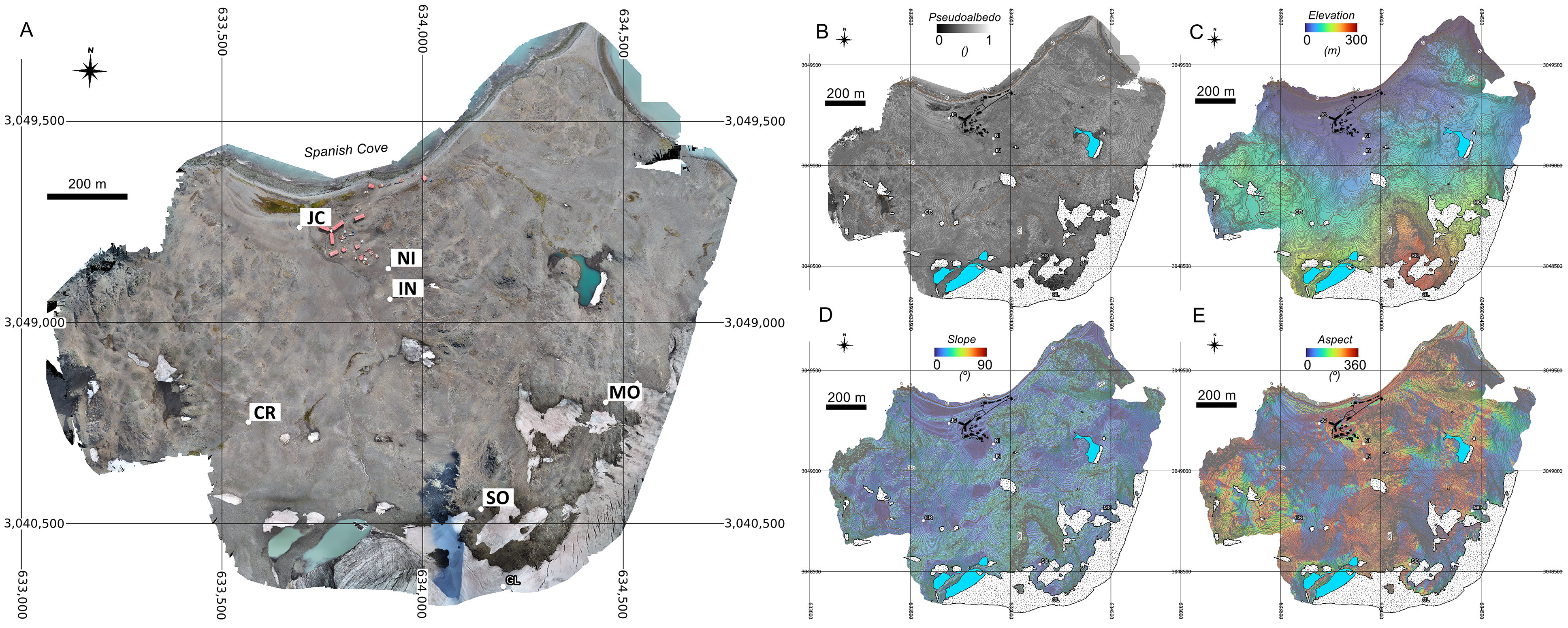
The UAV-derived terrain layers show a marked topographic contrast between the coastal sector around the SAS-JCI and the higher slopes toward Mount Reina Sofía (Figure 2). Elevation increases rapidly inland, and the slope and aspect maps reveal a heterogeneous relief with alternating gentle surfaces, steeper sectors and differently oriented slopes. The RGB-derived pseudoalbedo layer shows relative spatial variations in apparent surface brightness across the ice-free area, although these variations should not be interpreted as calibrated differences in broadband surface albedo.

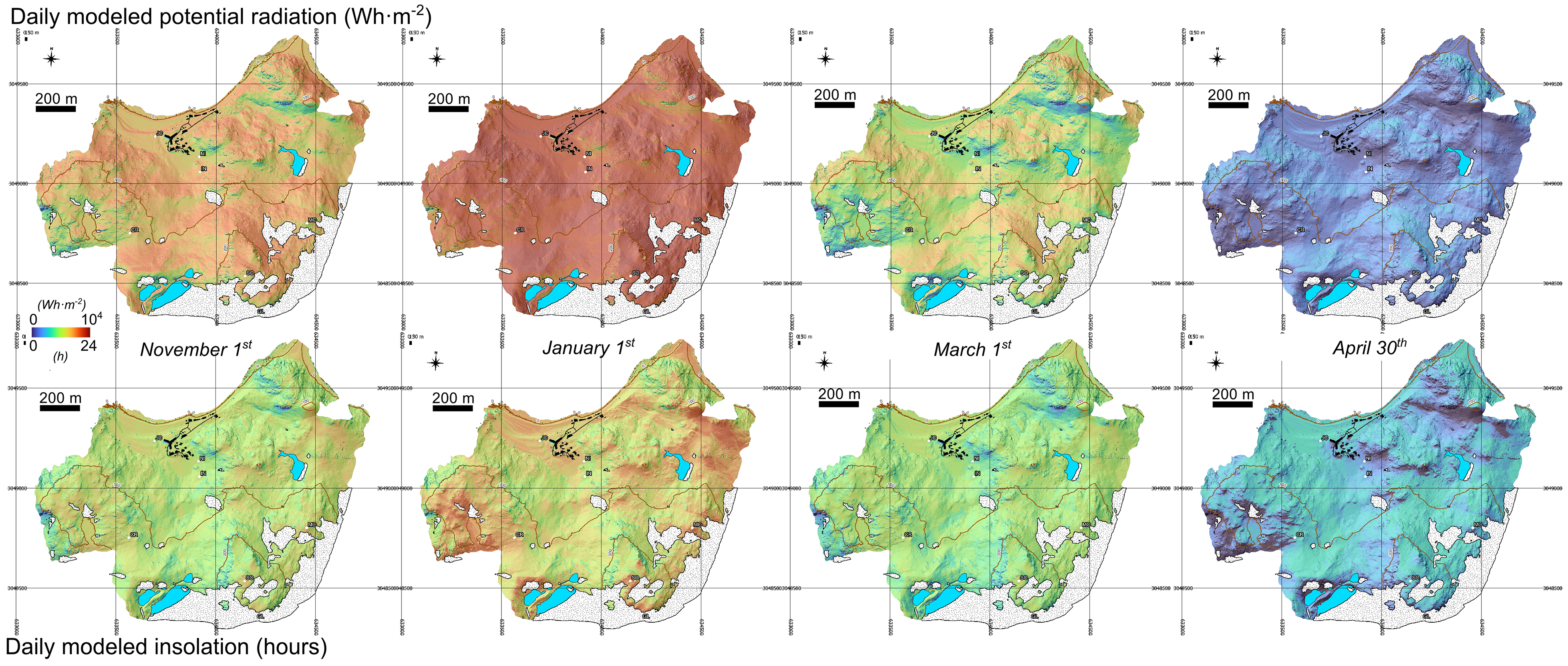
Modeled potential-radiation changes strongly through the thawing season (Figure 3). Values are lowest and more spatially contrasted at the beginning of November and toward late April, when low solar elevation enhances the effect of slope orientation and terrain shading. During the central summer period, especially from December to February, higher radiation values extend across most open and favorably oriented surfaces, while lower values persist in shaded slope sectors and locally obstructed terrain. The maps therefore show both a clear seasonal increase–decrease pattern and persistent spatial contrasts linked to local relief.

Potential insolation shows a related seasonal evolution, but its spatial pattern is not identical to that of modeled radiation (Figure 3). Areas with longer potential sunshine duration are mainly those with less topographic obstruction, whereas sectors affected by local shading show shorter exposure times. The differences between radiation and insolation maps are most evident at the beginning and end of the season, when low solar elevation increases the spatial contrast associated with slope orientation and local horizon effects. Together, the maps show that modeled potential radiation and insolation are spatially heterogeneous across the study area and that their internal contrasts vary markedly during the thawing season.

3.3. Modeled and Measured Radiation

When integrated over the thermally effective thawing periods, accumulated modeled potential radiation ranged from 428.125 to 832.984 Wh m⁻² (Table 2). The lowest value occurred at SO in 2023–2024, whereas the highest was recorded at JC in 2022–2023. Mean daily modeled potential radiation ranged from 5584 to 7837 Wh m⁻² d⁻¹, with the minimum at NI in 2022–2023 and the maximum at CR in 2024–2025. Accumulated potential insolation ranged from 970.0 to 1832.3 h, with the lowest value at IN in 2024–2025 and the highest at JC in 2022–2023. Mean daily potential insolation ranged from 11.33 to 16.90 h d⁻¹, with the minimum at NI in 2022–2023 and the maximum at SO in 2022–2023. These values were calculated over the same station-specific intervals used to derive the GST indices.

The accumulated values partly reflected the duration of the thermally effective thawing period, whereas the mean daily values better describe the average potential radiative conditions experienced by each station during its effective interval. For example, JC in 2022–2023 had the longest effective thawing period and consequently showed the highest accumulated modeled radiation and potential-insolation values, despite having intermediate mean daily potential conditions. In contrast, SO in 2023–2024 had the shortest effective period and showed the lowest accumulated modeled radiation, despite not having the lowest mean daily potential radiation (Table 2).

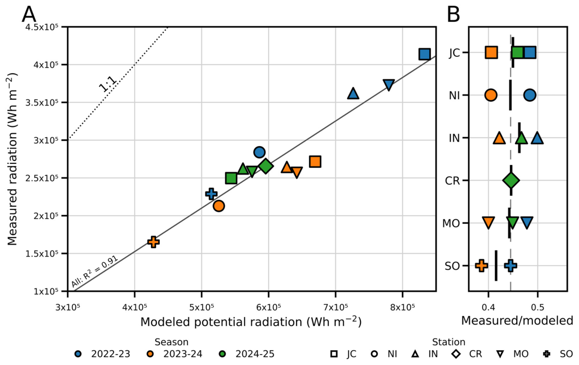
Measured solar radiation at the AEMET station was consistently lower than modeled potential radiation during the same thermally effective thawing periods (Figure 4). Because the AEMET station is located approximately 3 m from the JC GST sensor, the most direct comparison is between measured radiation and modeled potential radiation at JC. At this station, the measured-to-modeled accumulated radiation ratio was 0.50 in 2022–2023, 0.41 in 2023–2024 and 0.46 in 2024–2025. Across all station periods, the ratio ranged from 0.39 to 0.50, with a mean value of 0.45. These ratios indicate that measured incoming solar radiation was approximately 40–50% of modeled potential radiation over the analyzed effective thawing periods. Mean daily air temperature during the same periods ranged from 1.85 to 2.89 °C, as measured at the AEMET AWS. These measured meteorological data provide atmospheric context for the modeled-radiation analysis, but were not used to calibrate the potential-radiation model.

3.4. Thermal Intensity

Thermal intensity during the thermally effective thawing period varied across stations and seasons (Table 2). In the complete-period dataset, TDDm ranged from 2.2 to 5.8 °C, while mean daily GST showed nearly identical values. This similarity reflects the fact that most daily mean GST values within the objectively defined thermally effective thawing periods were positive. TDDm may be slightly higher than mean daily GST when an interval includes isolated days with daily mean GST at or below 0 °C (Table 2), because non-positive values do not contribute to accumulated TDD but are included in the calculation of mean GST. The lowest thermal-intensity values were recorded at SO in 2023–2024, whereas the highest values occurred at JC in 2024–2025. Maximum daily mean GST ranged from 5.8 to 12.8 °C, with the minimum again recorded at SO in 2023–2024 and the maximum at NI in 2022–2023.

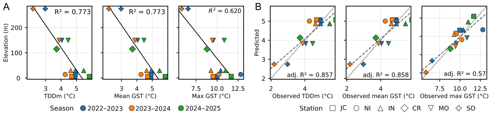
The strongest bivariate relationships for thermal-intensity variables were obtained with elevation (

Table 3. Selected bivariate relationships and empirical models for the main thermal components. Note: For bivariate relationships, the reported value is R². For empirical models, the reported value is adjusted R². RMSE and LOOCV RMSE are expressed in the units of the response variable. LOOCV = leave-one-out cross-validation. VIF = variance inflation factor; VIF values are reported only for multiple-predictor models. RADmean and RADtotal refer to modeled potential solar radiation. Models are empirical summaries of the station-year dataset and should not be interpreted as spatially distributed predictive models. Associations between timing variables and RADtotal are reported only as contextual relationships because RADtotal was integrated over the station-specific thermally effective thawing interval and should not be interpreted as an independent predictor of its timing.

Type	Component	Response	Predictor/Model	n	R2/Adj. R2	RMSE	MAE	VIF	LOOCV RMSE	Use
Bivariate	Intensity	TDDm	Elevation	14	0.773					Descriptive
		Mean GST	Elevation	14	0.773
		Max daily mean GST	Elevation	14	0.620
	Accumulation	TDD	Elevation	14	0.686					Contextual
		TDD	Duration	14	0.756
	Timing	Duration	RADtotal	14	0.768					Contextual
		Start DOY	RADtotal	14	0.719
Model	Intensity	TDDm	Elevation + RADmean	14	0.852	0.327	0.267	1.15	0.424	Primary
		Mean GST	Elevation + RADmean	14	0.858	0.320	0.259	1.15	0.414	Alternative
	Extremes	Max daily mean GST	Elevation + RADmean	14	0.573	1.062	0.859	1.15	1.395	Secondary
	Accumulation	TDD	Duration + Elevation	14	0.932	30.802	26.911	1.40	38.942	Supporting

; Figure 5). Elevation was negatively correlated with all thermal-intensity variables, indicating lower thermal-intensity values at higher stations. As expected from their closely related definitions, TDDm and mean daily GST showed identical relationships with elevation at the displayed precision, with R² values of 0.773 and 0.773, respectively. Maximum daily mean GST showed a weaker relationship with elevation, with R² = 0.620 (Table 3).

Simple empirical models combining elevation and mean modeled potential solar radiation provided the best fits for the main thermal-intensity variables (Table 3; Figure 5). The model combining elevation and mean modeled potential radiation explained TDDm with an adjusted R² of 0.852 and a leave-one-out cross-validation RMSE of 0.424 °C. A nearly identical result was obtained for mean daily GST, as expected from its close relationship with TDDm, with an adjusted R² of 0.858 and a leave-one-out cross-validation RMSE of 0.414 °C. For maximum daily mean GST, the model had an adjusted R² of 0.573 and a leave-one-out cross-validation RMSE of 1.395 °C (Table 3). Collinearity between elevation and RADmean was negligible, with VIF values of 1.15 for both predictors in the thermal-intensity models (Table 3).

3.5. Thermal Accumulation

Accumulated TDD during the thermally effective thawing period ranged from 146.4 to 614.7 °C·day across the complete-period dataset, with a mean value of 402.9 °C·day (Table 2). The lowest value was recorded at SO in 2023–2024, whereas the highest value occurred at JC in 2022–2023. In general, lower accumulated TDD values occurred at the highest-elevation station SO, while the largest values were recorded mainly at the lower-elevation stations JC, IN, and NI.

Accumulated TDD showed strong bivariate relationships with both elevation and duration, with R² values of 0.686 and 0.756, respectively (Table 3). The best empirical model for accumulated TDD combined duration and elevation, with an adjusted R² of 0.932, an RMSE of 30.8 °C·day, an MAE of 26.9 °C·day, and a leave-one-out cross-validation RMSE of 38.9 °C·day (Table 3). Collinearity between duration and elevation was also low in this model, with VIF values of 1.40 for both predictors (Table 3).

3.6. Secondary Controls

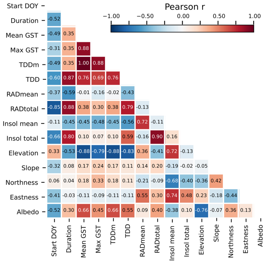
The correlation matrix showed that elevation had the strongest bivariate relationships with the thermal-intensity variables, whereas slope, aspect-derived variables and potential insolation showed weaker or less consistent relationships (Figure 6). Mean modeled potential radiation showed only weak bivariate relationships with thermal intensity, despite its contribution to the multivariable models when combined with elevation (Table 3; Figure 5). Slope showed its strongest relationship with the onset of the thermally effective thawing period, although this association remained weak, whereas its relationships with duration, thermal intensity, and accumulated TDD were lower. Aspect-derived variables, including northness and eastness, showed only weak or inconsistent correlations with most thermal components.

Pseudoalbedo showed some first-order relationships with thermal-intensity variables (Figure 6), but these are interpreted only as exploratory associations. These correlations were similar for TDDm and mean daily GST, as expected given that both variables describe mean thermal intensity over the same thermally effective interval. However, pseudoalbedo was not included in the main empirical models because it was derived from RGB imagery as an exploratory apparent-surface-brightness proxy rather than from calibrated radiometric measurements and therefore should not be interpreted as an independent radiative control.

Potential insolation showed different relationships depending on whether it was expressed as a mean daily value or as an accumulated value over the thermally effective thawing period (Figure 6). Mean daily potential insolation showed weaker relationships with thermal intensity than elevation, whereas accumulated potential insolation was more closely related to duration. This pattern was consistent with the correlation structure observed for accumulated modeled potential radiation, which was also strongly related to timing variables because both were calculated over the same interval. These relationships are therefore interpreted as contextual consequences of the station-specific integration window rather than as evidence that accumulated potential radiation or insolation independently controls the timing of the thermally effective thawing period.

3.7. Inter-Seasonal Comparison

Descriptive inter-seasonal differences were assessed using all complete station–season intervals included in the main dataset (

Table 4. Descriptive inter-seasonal comparison of the thermally effective thawing period for (A) all available complete station–season intervals and (B) the common-station subset including only stations with complete intervals in all three seasons.

A. All Available Complete Intervals
Metric	2022–2023	2023–2024	2024–2025
Complete station–season intervals	5	5	4
Stations	JC, NI, IN, MO, SO	JC, NI, IN, MO, SO	JC, IN, CR, MO
Onset range	29 November–25 December	15 December–7 January	10 December–15 December
End range	25 February–8 April	14 March–3 April	23 February–24 February
Mean duration (d)	105.8	90.2	74.2
Duration range (d)	68–131	67–103	71–76
Mean TDDm (°C)	4.4	3.9	4.9
Mean TDD (°C·day)	474.3	365.5	360.5
B. Common-Station Subset
Metric	2022–2023	2023–2024	2024–2025
Complete station–season intervals	3	3	3
Stations	JC, IN, MO	JC, IN, MO	JC, IN, MO
Onset range	29 November–5 December	15 December	11 December–15 December
End range	25 March–8 April	15 March–27 March	23 February–24 February
Mean duration (d)	118.7	96.7	73.7
Duration range (d)	112–131	91–103	71–76
Mean TDDm (°C)	4.6	4.4	5.3
Mean TDD (°C·day)	550.3	426.7	386.5

). Considering all available complete intervals, mean duration decreased from 105.8 days in 2022–2023 to 90.2 days in 2023–2024 and 74.2 days in 2024–2025. Mean TDD likewise decreased from 474.3 to 365.5 and 360.5 °C·day, respectively, whereas mean TDDm was lowest in 2023–2024 and highest in 2024–2025. Because station availability differed among seasons, particularly in 2024–2025, these seasonal summaries were complemented by a comparison restricted to JC, IN and MO, the three stations with complete intervals in all three seasons.

The common-station subset showed the same temporal pattern (Table 4). Mean duration decreased from 118.7 days in 2022–2023 to 96.7 days in 2023–2024 and 73.7 days in 2024–2025, while mean accumulated TDD decreased from 550.3 to 426.7 and 386.5 °C·day. In contrast, mean TDDm decreased slightly from 4.6 °C in 2022–2023 to 4.4 °C in 2023–2024 and increased to 5.3 °C in 2024–2025. At the individual-station level, JC, IN and MO all showed shorter effective thawing intervals and lower accumulated TDD in 2024–2025 than in 2022–2023, despite higher TDDm values in 2024–2025. Given the limited three-season record, these differences are described as inter-seasonal variability and are not interpreted as a temporal trend.

4. Discussion

4.1. Potential Radiation

The comparison between measured and modeled radiation is important for interpreting the role of the potential-radiation product used in this study. The modeled values were systematically higher than the radiation measured by the AEMET automatic weather station, with measured-to-modeled ratios between 0.39 and 0.50 across the analyzed station-years (Figure 4). This difference is expected because the model represents potential incoming radiation controlled by solar geometry and local terrain, whereas the measured record includes cloud cover, atmospheric attenuation, fog, wind-driven snow conditions and other short-term meteorological factors. DEM-derived radiation models are therefore best interpreted as spatial indices of potential energy availability rather than as direct estimates of the actual surface energy balance [43].

The comparison is most robust at JC because the AEMET station is located approximately 3 m from the JC GST sensor. At this station, the measured-to-modeled accumulated radiation ratio was 0.50 in 2022–2023, 0.41 in 2023–2024 and 0.46 in 2024–2025 (Figure 4). These values indicate that the potential-radiation model consistently overestimates actual incoming radiation, but also that the ratio between measured and modeled radiation remains relatively stable among seasons. For the remaining stations, the AEMET data should be interpreted only as a common low-elevation atmospheric reference, because local cloudiness, fog, wind exposure and orographic effects may differ along the altitudinal transect, although the small spatial extent of the study area suggests that these unmeasured meteorological differences are likely to be limited.

This distinction is especially relevant in maritime Antarctica, where frequent cloudiness, strong winds, and rapidly changing weather conditions strongly affect incoming shortwave radiation and surface energy exchanges [20,29]. The measured radiation data therefore do not invalidate the modeled product; rather, they clarify its meaning. The model does not quantify the actual radiation received at each station, but it provides a consistent topographic and astronomical framework for comparing the relative potential energy availability imposed by elevation, slope, aspect and terrain shading (Figure 3). This interpretation is appropriate for remote monitoring networks where radiometers are rarely available at every GST station, but high-resolution UAV-derived topography can be used to characterize spatial contrasts in potential radiation. Future studies could refine and validate this approach by incorporating radiative-transfer modeling that explicitly represents atmospheric attenuation, diffuse radiation and terrain-reflection effects, and by comparison with remote-sensing-based radiation products where these are available at appropriate spatial and temporal resolution.

4.2. Effective Coupling

Once modeled radiation is interpreted as potential rather than actual incoming energy, its relationship with GST must be considered within the part of the seasonal cycle in which the ground surface can respond thermally to that forcing. In snow-affected cold-region surfaces, GST does not necessarily increase in parallel with incoming radiation because snow cover can decouple the ground from atmospheric and radiative forcing by modifying albedo, insulation and conductive heat transfer [6,16]. After snowmelt, GST may also remain close to 0 °C while available energy is consumed by water–ice phase changes in the near-surface ground, producing zero-curtain-like behavior [17]. Similar phase-based thermal behavior has been described in alpine and Antarctic GST records, where the transition from the zero-curtain phase to the warm phase marks the onset of a more direct positive-temperature response of the ground surface [23,25,26].

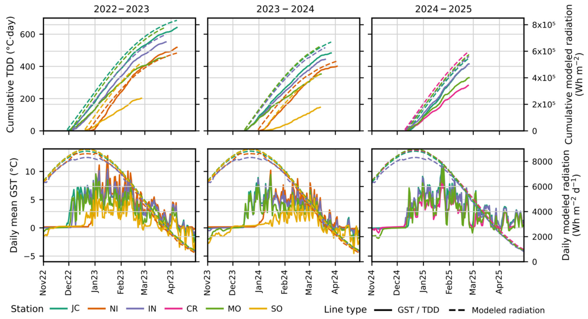
The results support the need to analyze this thermally effective interval separately. The onset of the effective thawing period varied from 29 November to 7 January, and therefore did not coincide with a fixed astronomical or calendar date (Table 2; Figure 7). Modeled potential radiation was already high before several stations entered the thermally effective thawing period, whereas TDD and effective accumulated radiation only began to increase from the station-specific onset dates (Figure 7). The temporal offset between high-potential radiation and the onset of sustained GST warming therefore reflects the fact that part of the summer radiative forcing occurs while the ground surface is still buffered by snowmelt or near-0 °C phase-change processes. This pattern is consistent with the influence of thermally buffered conditions preceding the sustained positive-temperature response identified by the objective criterion, but their duration and controlling processes were not quantified here. Consequently, the thermal effect of modeled potential radiation must be evaluated over the station-specific effective thawing period rather than over the full summer season.

This approach also helps separate timing, thermal intensity and thermal accumulation. Accumulated TDD is a standard integrated index in cold-region and permafrost studies, and its dependence on both the magnitude and duration of positive temperatures is inherent to its definition [13,35,36]. The relevant point here is therefore not that longer or warmer intervals produce higher TDD, but that TDD, modeled potential radiation and potential insolation were all integrated over the same station-specific thermally effective interval, avoiding the inclusion of snowmelt or zero-curtain-like conditions in cumulative indices (Table 2; Figure 7).

The descriptive inter-seasonal comparison further illustrates the need to distinguish thermal intensity from thermal accumulation. Considering all available complete station–season intervals, the 2024–2025 season showed the highest mean daily thawing intensity, expressed as TDDm (4.9 °C), but also the shortest mean effective thawing interval (74.2 days), resulting in a lower mean accumulated TDD than in 2022–2023 (360.5 versus 474.3 °C·day). This pattern was also observed when the comparison was restricted to JC, IN and MO, the three stations with complete intervals in all three seasons: 2024–2025 showed a higher mean TDDm than 2022–2023 (5.3 versus 4.6 °C), but a shorter mean effective interval (73.7 versus 118.7 days) and lower mean accumulated TDD (386.5 versus 550.3 °C·day) (Table 4). Thus, the higher mean thawing intensity recorded in 2024–2025 did not compensate for the shorter duration of the thermally effective interval. Although the common-station comparison reduces the influence of differences in station availability among seasons, these contrasts are interpreted as inter-seasonal variability rather than as evidence of a temporal trend, because only three seasons were available.

The separation between timing, intensity and accumulation also places the present results within the broader PERMATHERMAL framework. Previous studies in Livingston and Deception Islands showed that GST regimes are strongly modulated by snow cover and zero-curtain phases, and that recent warming is expressed not only as higher temperatures but also as changes in the duration and frequency of thermal regimes [22,23]. The present analysis complements those results by focusing on the interval after snowmelt and zero-curtain-like conditions, when topographic and radiative controls can be more directly compared with the observed GST response (Figure 7). Thus, modeled potential radiation is not used to explain the whole annual GST cycle, but specifically the period in which the ground surface is thermally available to respond to radiative and topographic forcing.

4.3. Thermal Intensity

The empirical analysis shows that the mean thermal intensity of the effective thawing period was most clearly organized by elevation, whereas mean modeled potential radiation contributed only as part of models that also included elevation. TDDm and mean GST both decreased clearly with elevation, whereas maximum daily mean GST showed a weaker relationship (Table 3; Figure 5). This distinction suggests that elevation better explains the average thermal state reached by the ground surface after snowmelt or zero-curtain-like conditions, while short-lived maximum values are more sensitive to transient meteorological and surface conditions.

The dominance of elevation is consistent with previous work in Hurd Peninsula and other ice-free sectors of Livingston Island, where altitudinal gradients have been linked to air temperature, ground thermal regimes, freezing and thawing indices, and permafrost distribution [13,21,23,53]. However, elevation should not be interpreted only as a lapse-rate proxy. Along this short transect, it also integrates changes in wind exposure, snow redistribution, snow persistence, surface moisture and the timing of the transition from snowmelt or zero-curtain-like conditions to sustained positive GST. Similar combined controls have been reported in maritime Antarctica, where GST regimes are shaped by interactions among topography, snow cover, atmospheric forcing and surface conditions rather than by a single factor alone [7,14,23,54,55]. This altitudinal organization is also consistent with previous interpretations of Hurd Peninsula as a marginal permafrost environment, where lower coastal sectors are generally permafrost-free or weakly affected by frozen ground, whereas higher-elevation areas are more favorable for warm or discontinuous permafrost conditions [13,21,23].

Although mean modeled potential radiation showed little independent bivariate association with thermal intensity, it was retained alongside elevation in the best-fitting empirical models for TDDm and mean GST (Table 3; Figure 5 and Figure 6). This is physically coherent with the definition of the thermally effective thawing period: once the ground surface has entered a sustained positive-temperature response, local potential radiation can modulate surface warming, but within a thermal framework already structured by elevation, snow history and the timing of effective exposure. The weaker model performance for maximum daily mean GST further suggests that short-term thermal peaks depend on additional factors, such as transient clear-sky conditions, abrupt snow changes, surface wetness or wind exposure, which are not captured by seasonal mean potential radiation and elevation alone [7,8,14,23].

The limited role of slope and aspect-derived variables at the station scale should be interpreted in relation to the specific location of the monitoring sites, which are mostly placed on locally gentle to moderately sloping, wind-exposed surfaces. Although the study area is spatially restricted and most monitoring sites occupy a comparatively limited altitudinal range, the inclusion of SO extends the transect to a distinctly higher-elevation setting. Within this local-scale context, the UAV-derived maps show terrain-related spatial differences in modeled radiation and insolation (Figure 2 and Figure 3). At the monitored sites, however, these terrain effects are expressed more clearly through modeled potential radiation than through slope or aspect considered independently (Figure 6). Thus, the contribution of the UAV-derived radiation model is not to replace elevation as the main predictor, but to integrate local terrain geometry into the interpretation of thermal intensity once the thermally effective thawing period has been isolated (Table 3; Figure 5 and Figure 6).

4.4. Secondary Controls

The correlation matrix confirms that elevation had the clearest bivariate relationships with the main thermal-intensity indices, whereas slope, aspect-derived variables, potential insolation and RADmean showed weaker or less consistent independent relationships (Figure 6). This does not mean that these variables are physically irrelevant, but that their independent statistical signal was limited within the monitored transect. Slope and aspect contribute to the spatial structure of modeled radiation, whereas RADmean provided additional information only when considered together with elevation in the multivariable thermal-intensity models (Table 3; Figure 5 and Figure 6).

Potential insolation and pseudoalbedo should therefore be interpreted as contextual variables rather than primary predictors. Insolation time describes potential sunlight duration, but not the energetic magnitude of incoming radiation. Pseudoalbedo showed moderate relationships with some thermal-intensity variables, but it was derived from RGB UAV imagery and cannot be treated as calibrated broadband albedo. Surface properties can influence ground thermal regimes in Antarctic ice-free terrain through energy absorption, moisture and snow persistence [7,54,55], but in this analysis, pseudoalbedo remains an exploratory surface descriptor.

Thus, the value of Figure 6 is mainly diagnostic. It supports the choice of simple empirical models combining elevation and RADmean, while showing that the remaining terrain and surface descriptors did not provide a stronger independent signal within the available station-year dataset.

4.5. Spatial Implications

The mapped radiation and insolation products are a key outcome of the UAV–GIS workflow because they transform the high-resolution DEM into spatially continuous layers of potential energy availability (Figure 2 and Figure 3). Within this spatially restricted study area, these layers reveal terrain-related differences in potential energy availability that are not fully represented by station elevation alone. They therefore provide the spatial framework required to move from point GST observations toward a distributed interpretation of ground-surface thermal regimes.

However, the results also show that potential-radiation maps cannot be translated directly into maps of GST response or accumulated TDD. The station analysis indicates that modeled radiation is physically meaningful when evaluated over the thermally effective thawing period, but the objectively defined onset and end of this interval differed among stations and seasons (Table 2; Figure 7). Therefore, the critical missing spatial variable for a distributed TDD model is not potential radiation alone, but the duration of the thermally effective period at each location, which is expected to depend largely on snow-cover duration, as well as on surface moisture and near-surface soil characteristics.

A simple GIS-based model of accumulated ground-surface thawing would require two spatial components. The first is a map of mean daily thawing intensity during the thermally effective thawing period, constrained by GST observations and by predictors supported by the present empirical analysis, particularly elevation and, in combination with elevation, mean modeled potential radiation. The second is a map of the duration of that effective period. Only by combining both components could a distributed TDD layer be produced:

$$TDD(x,y)=TDDm(x,y)\cdot D(x,y)$$

(2)

where $TDDm(x,y)$ represents the predicted mean daily thawing-degree–day contribution during the thermally effective period and $D(x,y)$ its spatially variable duration of that interval.

This distinction defines the next methodological step. The present results provide a first-order empirical basis for estimating the spatial differences in mean daily thawing intensity, whereas the spatial duration of the thermally effective thawing period remains to be determined. Additional GST sensors, spatial information on snow-cover persistence and thermal-transition timing, repeated UAV or satellite observations, or terrain-based snow-persistence indicators would be needed to estimate the spatial duration of the effective thawing period. Once this duration component is available, distributed TDD estimates could be linked with soil thermal properties or edaphic factors through Stefan-type approaches to explore spatial differences in active-layer thawing potential [35,56]. Systematic measurements of active-layer thickness and soil thermal properties at representative geomorphological units would then be needed to calibrate local edaphic factors and move from ground-surface thermal forcing toward spatial estimates of thaw depth. The present study therefore does not provide a map of active-layer thickness or permafrost probability; instead, it establishes the radiative, topographic and thermal framework required to develop such a spatial model.

5. Conclusions

The main implication of this study is that the thermally effective GST thawing period should be treated as the relevant analytical window for evaluating radiative and topographic controls on ground-surface warming in snow-affected maritime Antarctic terrain. This interval varied among stations and seasons and did not coincide with a fixed calendar or astronomical window. Defining it objectively from GST records was therefore necessary to exclude snowmelt and zero-curtain-like conditions from the analysis.

The comparison with AEMET measurements confirms that DEM-derived radiation products should be interpreted as indices of terrain-controlled potential energy availability, not as estimates of actual incoming shortwave radiation or surface energy balance. Nevertheless, the modeled radiation and insolation maps provided a consistent spatial framework for evaluating terrain-controlled potential energy availability across the study area rather than a direct estimate of actual surface energy balance.

Thermal intensity during the effective thawing period was not explained by potential radiation alone, but by a local environmental framework in which elevation acted as the dominant organizing variable and modeled potential radiation provided secondary information when combined with elevation. Slope, aspect, potential insolation and pseudoalbedo acted mainly as contextual variables at the monitored sites, although they contributed to the broader spatial structure of modeled radiation and insolation.

For spatial modeling, the key conclusion is that accumulated ground-surface thawing cannot be inferred from potential radiation or mean thermal intensity alone, because the duration of the thermally effective period is an equally necessary component. Calculating TDD, modeled radiation and potential insolation over the same station-specific intervals allowed consistent comparison among stations and avoided mixing radiative forcing that occurred before the ground surface was thermally available to respond.

The UAV–GIS–GST workflow provides a practical first-order framework for linking point GST observations with high-resolution spatial information in remote Antarctic environments. Its main limitations are the small number of complete station-year periods, the absence of spatially distributed measurements of actual incoming radiation and snow-cover duration, and the empirical nature of the models. Future work toward distributed TDD or active-layer modeling will require spatial estimates of the duration of the thermally effective thawing period, supported by additional GST sensors, snow-free timing information, repeated remote observations or terrain-based snow-persistence indicators. Such estimates should account for snow-cover duration and other local factors, including surface moisture and near-surface soil characteristics.

References

1. Vieira, G.; Bockheim, J.; Guglielmin, M.; Balks, M.; Abramov, A.A.; Boelhouwers, J.; Cannone, N.; Ganzert, L.; Gilichinsky, D.A.; Goryachkin, G.; et al. Thermal state of permafrost and active-layer monitoring in the Antarctic: Advances during the International Polar Year 2007–2009. Permafr. Periglac. Process. 2010, 21, 182–197. [Google Scholar] [CrossRef]
2. Bockheim, J.; Vieira, G.; Ramos, M.; López-Martínez, J.; Serrano, E.; Guglielmin, M.; Wilhelm, K.; Nieuwendam, A. Climate warming and permafrost dynamics in the Antarctic Peninsula region. Glob. Planet. Change 2013, 100, 215–223. [Google Scholar] [CrossRef]
3. Biskaborn, B.K.; Smith, S.L.; Noetzli, J.; Matthes, H.; Vieira, G.; Streletskiy, D.A.; Schoeneich, P.; Romanovsky, V.E.; Lewkowicz, A.G.; Abramov, A.; et al. Permafrost is warming at a global scale. Nat. Commun. 2019, 10, 264. [Google Scholar] [CrossRef]
4. Obu, J.; Westermann, S.; Vieira, G.; Abramov, A.; Balks, M.R.; Bartsch, A.; Hrbáček, F.; Kääb, A.; Ramos, M. Pan-Antarctic map of near-surface permafrost temperatures at 1 km2 scale. Cryosphere 2020, 14, 497–519. [Google Scholar] [CrossRef]
5. Hrbáček, F.; Oliva, M.; Hansen, C.; Balks, M.; O’Neill, T.A.; de Pablo, M.A.; Ponti, S.; Ramos, M.; Vieira, G.; Abramov, A.; et al. Active layer and permafrost thermal regimes in the ice-free areas of Antarctica. Earth-Sci. Rev. 2023, 242, 104458. [Google Scholar] [CrossRef]
6. Zhang, T. Influence of the seasonal snow cover on the ground thermal regime: An overview. Rev. Geophys. 2005, 43, RG4002. [Google Scholar] [CrossRef]
7. Hrbáček, F.; Oliva, M.; Láska, K.; Ruiz-Fernández, J.; de Pablo, M.A.; Vieira, G.; Ramos, M.; Nývlt, D. Active layer thermal regime in two climatically contrasted sites of the Antarctic Peninsula region. Cuad. Investig. Geogr. 2016, 42, 457–474. [Google Scholar] [CrossRef][Green Version]
8. Hrbáček, F.; Engel, Z.; Kňažková, M.; Smolíková, J. Effect of summer snow cover on the active layer thermal regime and thickness on CALM-S JGM site, James Ross Island, eastern Antarctic Peninsula. Catena 2021, 207, 105608. [Google Scholar] [CrossRef]
9. Sancho, L.G.; Pintado, A.; Navarro, F.; Ramos, M.; de Pablo, M.A.; Blanquer, J.M.; Raggio, J.; Valladares, F.; Green, T.G.A. Recent warming and cooling in the Antarctic Peninsula region has rapid and large effects on lichen vegetation. Sci. Rep. 2017, 7, 5689. [Google Scholar] [CrossRef]
10. de Pablo, M.A.; Molina, A.; Recio, C.; Ramos, M.; Goyanes, G.; Ropero, M.A. Análisis del estado de la capa activa en el emplazamiento de la base antártica española Gabriel de Castilla, Isla Decepción, Antártida. Bol. Geol. Min. 2017, 128, 69–92. [Google Scholar] [CrossRef]
11. Cannone, N.; Malfasi, F.; Favero-Longo, S.E.; Convey, P.; Guglielmin, M. Acceleration of climate warming and plant dynamics in Antarctica. Curr. Biol. 2022, 32, 1599–1606.e2. [Google Scholar] [CrossRef]
12. Ishikawa, M. Thermal regimes at the snow-ground interface and their implications for permafrost investigation. Geomorphology 2003, 52, 105–120. [Google Scholar] [CrossRef]
13. Ferreira, A.; Vieira, G.; Ramos, M.; Nieuwendam, A. Ground temperature and permafrost distribution in Hurd Peninsula (Livingston Island, Maritime Antarctic): An assessment using freezing indexes and TTOP modelling. Catena 2017, 149, 560–571. [Google Scholar] [CrossRef]
14. Baptista, J.; Vieira, G.; Lee, H. Ground surface temperature regimes are controlled by the topography and snow cover in the ice-free areas of Maritime Antarctica. Catena 2024, 240, 107947. [Google Scholar] [CrossRef]
15. Baptista, J.P.; Westermann, S.; Aas, K.S.; Schuler, T.V.; Etzelmüller, B. Modelling the evolution of permafrost temperatures and active layer thickness in King George Island, Antarctica, since 1950. Cryosphere 2025, 19, 3459–3476. [Google Scholar] [CrossRef]
16. Goodrich, L.E. The influence of snow cover on the ground thermal regime. Can. Geotech. J. 1982, 19, 421–432. [Google Scholar] [CrossRef]
17. Outcalt, S.I.; Nelson, F.E.; Hinkel, K.M. The zero-curtain effect: Heat and mass transfer across an isothermal region in freezing soil. Water Resour. Res. 1990, 26, 1509–1516. [Google Scholar] [CrossRef]
18. de Pablo, M.A.; Ramos, M.; Molina, A. Thermal characterization of the active layer at the Limnopolar Lake CALM-S site on Byers Peninsula (Livingston Island), Antarctica. Solid Earth 2014, 5, 721–739. [Google Scholar] [CrossRef]
19. de Pablo, M.A.; Ramos, M.; Molina, A.; Prieto, M. Thaw depth spatial and temporal variability at the Limnopolar Lake CALM-S site, Byers Peninsula, Livingston Island, Antarctica. Sci. Total Environ. 2018, 615, 814–827. [Google Scholar] [CrossRef]
20. Bañón, M.; Vasallo, F. AEMET en la Antártida: Climatología y Meteorología Sinóptica en las Estaciones Meteorológicas Españolas en la Antártida; Agencia Estatal de Meteorología: Madrid, Spain, 2015; 152p. [Google Scholar]
21. Ramos, M.; Vieira, G.; de Pablo, M.A.; Molina, A.; Jiménez, J.J. Transition from a subaerial to a subnival permafrost temperature regime following increased snow cover (Livingston Island, Maritime Antarctica). Atmosphere 2020, 11, 1332. [Google Scholar] [CrossRef]
22. de Pablo, M.A.; Ramos, M.; Vieira, G.; Molina, A.; Ramos, R.; Maior, C.N.; Prieto, M.; Ruiz-Fernández, J. Interannual variability of ground surface thermal regimes in Livingston and Deception Islands (Maritime Antarctica) from 2007 to 2021. Land Degrad. Dev. 2024, 35, 378–393. [Google Scholar] [CrossRef]
23. de Pablo, M.A.; Ramos, M.; Vieira, G.; Molina, A.; Ruiz-Fernández, J. Thermal regimes and phases of surface temperature in Livingston and Deception Islands, Antarctica, 2007–2021: Influence of snow cover and implications for frozen ground. Antarct. Sci. 2025, 37, 413–426. [Google Scholar] [CrossRef]
24. de Pablo, M.A.; Goyanes, G. Temporal decomposition of near-surface air temperature in maritime Antarctica: Seasonality, trend and residual variability across Livingston and Deception Islands. Antarct. Sci. 2026. under review. [Google Scholar]
25. Delaloye, R. Contribution à L’étude du Pergélisol de Montagne en Zone Marginale. Ph.D. Thesis, GeoFocus, Université de Fribourg, Fribourg, Switzerland, 2004. Volume 10. 240p. [Google Scholar]
26. Schoeneich, P. GST: Ground Surface Temperature. Guidelines for Monitoring, Version 3; Permanent: Bolzano, Italy, 2011. [Google Scholar]
27. Bañón, M. El clima en la zona de influencia de la Base Antártica Española Juan Carlos I. Pap. Geogr. 1994, 20, 27–47. [Google Scholar]
28. Bañón, M. Observaciones meteorológicas en la Base Antártica Española Juan Carlos I; Monografía A-151; Instituto Nacional de Meteorología, Ministerio de Medio Ambiente: Madrid, Spain, 2001; 135p. [Google Scholar]
29. González-Herrero, S.; González-Espejo, I.; Jiménez-Cavero, C.M.; Albero-Molina, J.V.; Bañón, M.; Aguilar-Pérez, J.B.; Alcántara-Ruiz, A.; Bueno-Ferrer, J.M.; Casabella-Carbares, N.; Collado-Aceituno, J.L.; et al. Thirty-five years of Spanish atmospheric observations at Livingston and Deception Islands, South Shetland Islands, Antarctica. Antarct. Sci. 2026, 38, 57–72. [Google Scholar] [CrossRef]
30. Ramos, M.; Vieira, G.; Gruber, S.; Blanco, J.J.; Hauck, C.; Hidalgo, M.A.; Tomé, D.; Neves, M.; Trindade, A. Permafrost and active layer monitoring in the Maritime Antarctic: Preliminary results from CALM sites on Livingston and Deception Islands. In Antarctica: A Keystone in a Changing World—Online Proceedings of the 10th ISAES; Open-File Report 2007-1047, Short Research Paper 070; Cooper, A.K., Raymond, C.R., Eds.; U.S. Geological Survey: Reston, VA, USA, 2007; pp. 1–5. [Google Scholar] [CrossRef]
31. Bañón, M.; Justel, A.; Velázquez, D.; Quesada, A. Regional weather survey on Byers Peninsula, Livingston Island, South Shetland Islands, Antarctica. Antarct. Sci. 2013, 25, 146–156. [Google Scholar] [CrossRef]
32. de Pablo, M.A.; Ramos, M.; Molina, A.; Vieira, G.; Hidalgo, M.A.; Prieto, M.; Jiménez, J.J.; Fernández, S.; Recondo, C.; Calleja, J.F.; et al. Frozen ground and snow cover monitoring in the South Shetland Islands, Antarctica: Instrumentation, effects on ground thermal behavior and future research. Cuad. Investig. Geogr. 2016, 42, 475–495. [Google Scholar] [CrossRef]
33. de Pablo, M.A. Maintenance of PT and CALM stations for Permafrost and Active Layer Monitoring on Livingston and Deception Islands, Antarctica. 2024–25 Campaign Report; ACMA-Universidad de Alcalá: Alcalá de Henares, Spain, 2025; 74p. (In Spanish) [Google Scholar]
34. Choler, P.; Bonfanti, N.; Reverdy, A.; Bayle, A.; Nicoud, B.; Liger, L.; Clément, J.-C.; Cohard, J.-M.; Corona, C.; Gascoin, S.; et al. Legacy of snow cover on alpine landscapes. Commun. Earth Environ. 2025, 6, 758. [Google Scholar] [CrossRef]
35. Lunardini, V.J. Heat Transfer in Cold Climates; Van Nostrand Reinhold: New York, NY, USA, 1981. [Google Scholar]
36. Nelson, F.E.; Anisimov, O.A.; Shiklomanov, N.I. Climate change and hazard zonation in the circum-Arctic permafrost regions. Nat. Hazards 2002, 26, 203–225. [Google Scholar] [CrossRef]
37. Bash, E.A.; Moorman, B.J. Surface melt and the importance of water flow—An analysis based on high-resolution unmanned aerial vehicle (UAV) data for an Arctic glacier. Cryosphere 2020, 14, 549–563. [Google Scholar] [CrossRef]
38. Svensgaard, J.; Jensen, S.M.; Christensen, S.; Rasmussen, J. The importance of spectral correction of UAV-based phenotyping with RGB cameras. Field Crops Res. 2021, 269, 108177. [Google Scholar] [CrossRef]
39. Bartmiński, P.; Siłuch, M. Mapping the albedo of the active surface at different stages of the growing season using data from various sources. Remote Sens. Appl. Soc. Environ. 2022, 28, 100818. [Google Scholar] [CrossRef]
40. Ryan, J.C.; Hubbard, A.; Box, J.E.; Brough, S.; Cameron, K.; Cook, J.M.; Cooper, M.; Doyle, S.H.; Edwards, A.; Holt, T.; et al. Derivation of high spatial resolution albedo from UAV digital imagery: Application over the Greenland Ice Sheet. Front. Earth Sci. 2017, 5, 40. [Google Scholar] [CrossRef]
41. McCune, B.; Keon, D. Equations for potential annual direct incident radiation and heat load. J. Veg. Sci. 2002, 13, 603–606. [Google Scholar] [CrossRef]
42. Amatulli, G.; Domisch, S.; Tuanmu, M.-N.; Parmentier, B.; Ranipeta, A.; Malczyk, J.; Jetz, W. A suite of global, cross-scale topographic variables for environmental and biodiversity modeling. Sci. Data 2018, 5, 180040. [Google Scholar] [CrossRef]
43. Neteler, M.; Mitasova, H. Open Source GIS: A GRASS GIS Approach; Kluwer Academic Publishers: Boston, MA, USA, 2002. [Google Scholar]
44. Pearson, K. Note on regression and inheritance in the case of two parents. Proc. R. Soc. Lond. 1895, 58, 240–242. [Google Scholar] [CrossRef]
45. Babyak, M.A. What you see may not be what you get: A brief, nontechnical introduction to overfitting in regression-type models. Psychosom. Med. 2004, 66, 411–421. [Google Scholar] [CrossRef]
46. Burnham, K.P.; Anderson, D.R. Model Selection and Multimodel Inference: A Practical Information-Theoretic Approach, 2nd ed.; Springer: New York, NY, USA, 2002. [Google Scholar] [CrossRef]
47. Dormann, C.F.; Elith, J.; Bacher, S.; Buchmann, C.; Carl, G.; Carré, G.; Marquéz, J.R.G.; Gruber, B.; Lafourcade, B.; Leitão, P.J.; et al. Collinearity: A review of methods to deal with it and a simulation study evaluating their performance. Ecography 2013, 36, 27–46. [Google Scholar] [CrossRef]
48. Willmott, C.J.; Matsuura, K. Advantages of the mean absolute error (MAE) over the root mean square error (RMSE) in assessing average model performance. Clim. Res. 2005, 30, 79–82. [Google Scholar] [CrossRef]
49. Stone, M. Cross-validatory choice and assessment of statistical predictions. J. R. Stat. Soc. Ser. B 1974, 36, 111–133. [Google Scholar] [CrossRef]
50. Posit Team. RStudio: Integrated Development Environment for R; Posit Software, PBC: Boston, MA, USA, 2025. [Google Scholar]
51. OpenAI. ChatGPT (GPT-5.5 Thinking) [Large Language Model]. Available online: https://chatgpt.com/ (accessed on 19 May 2026).
52. Inkscape Project. Inkscape, Version 1.4.3. Available online: https://inkscape.org/release/inkscape-1.4.3/ (accessed on 26 May 2026).
53. Ramos, M.; Vieira, G.; de Pablo, M.A.; Molina, A.; Abramov, A.; Goyanes, G. Recent shallowing of the thaw depth at Crater Lake, Deception Island, Antarctica (2006–2014). Catena 2017, 149, 519–528. [Google Scholar] [CrossRef]
54. Guglielmin, M. Ground surface temperature (GST), active layer and permafrost monitoring in continental Antarctica. Permafr. Periglac. Process. 2006, 17, 133–143. [Google Scholar] [CrossRef]
55. Oliva, M.; Navarro, F.; Hrbáček, F.; Hernández, A.; Nývlt, D.; Pereira, P.; Ruiz-Fernández, J.; Trigo, R. Recent regional climate cooling on the Antarctic Peninsula and associated impacts on the cryosphere. Sci. Total Environ. 2017, 580, 210–223. [Google Scholar] [CrossRef] [PubMed]
56. Smith, M.W.; Riseborough, D.W. Climate and the limits of permafrost: A zonal analysis. Permafr. Periglac. Process. 2002, 13, 1–15. [Google Scholar] [CrossRef]
Figure 1. Location and field setting of the study area. (A) Location of Livingston Island within the South Shetland Islands, North-western Antarctic Peninsula region, with the position of the study area indicated near the Spanish Antarctic Station Juan Carlos I. (B) UAV oblique view of the SAS-JCI surroundings on Hurd Peninsula, showing the relative position of the PERMATHERMAL monitoring stations used in this study, the AEMET automatic weather station, and the main local toponymy.
Atmosphere 17 00602 g001
Figure 2. UAV-derived orthomosaic and terrain/surface products for the SAS-JCI study area on Hurd Peninsula, Livingston Island. (A) Orthomosaic showing the location of the PERMATHERMAL monitoring stations and the main local toponymy. (B) RGB-based pseudoalbedo derived from the orthomosaic, (C) elevation, (D) slope, and (E) aspect derived from the UAV digital elevation model.
Atmosphere 17 00602 g002
Figure 3. Seasonal evolution of daily modeled potential radiation (top row, in Wh m−2) and potential insolation (bottom row, in h) across the SAS-JCI study area, for selected dates between 1 November and 30 April. The selected dates provide a comparative overview of the seasonal spatial patterns of both potential-radiation products.
Atmosphere 17 00602 g003
Figure 4. Comparison between measured solar radiation at the AEMET automatic weather station at SAS-JCI and modeled potential solar radiation during the thermally effective thawing periods. (A) Accumulated measured versus modeled potential radiation, including the 1:1 line and linear fits for all station-periods. (B) Measured-to-modeled accumulated radiation ratio by station and season.
Atmosphere 17 00602 g004
Figure 5. Main thermal-intensity relationships and empirical models. (A) Relationships between elevation and TDDm, mean GST, and maximum daily mean GST. Solid lines represent the fitted linear relationships, and the corresponding coefficients of determination are shown in each plot. (B) Observed versus predicted values for the models based on elevation and mean modeled potential solar radiation. Dotted lines indicate the 1:1 reference relationship, whereas dashed lines represent the fitted relationships between observed and predicted values. Adjusted coefficients of determination are shown for the corresponding empirical models.
Atmosphere 17 00602 g005
Figure 6. Pearson correlation matrix for timing, thermal, radiative, insolation, and topographic variables calculated for the thermally effective thawing periods. Cell values indicate Pearson’s correlation coefficient (r) calculated for the thermally effective thawing periods. Pseudoalbedo is included only as an exploratory RGB-derived descriptor of apparent surface brightness; it is not calibrated broadband albedo and was not used as a predictor in the empirical models.
Atmosphere 17 00602 g006
Figure 7. Temporal evolution of GST-derived thermal indices and modeled potential radiation during the three analyzed thawing seasons. Upper panels show cumulative TDD and cumulative modeled potential radiation, both accumulated from the station-specific onset of the thermally effective thawing period. Lower panels show daily mean GST and daily modeled potential radiation from November to May. Solid lines represent GST-derived variables, and dashed lines represent modeled potential radiation.
Atmosphere 17 00602 g007