Article

On the Mechanical and Thermodynamic Influences of Ocean Spray in Hurricane Boundary Layers

1
Department of Mathematics & Statistics and Applied Science & Technology Ph.D. Program, North Carolina A&T State University, 302 Gibbs Hall, 1601 E. Market Street, Greensboro, NC 27411, USA
2
Department of Mathematics, Swinburne University of Technology, Hawthorn, VIC 3122, Australia
3
Department of Mathematics & Statistics, North Carolina A&T State University, 302 Gibbs Hall, 1601 E. Market Street, Greensboro, NC 27411, USA
*
Author to whom correspondence should be addressed.
Atmosphere 2026, 17(6), 559; https://doi.org/10.3390/atmos17060559 (registering DOI)
Submission received: 31 March 2026 / Revised: 26 May 2026 / Accepted: 27 May 2026 / Published: 29 May 2026
(This article belongs to the Section Meteorology)

Abstract

This study investigates the mechanical and thermodynamic effects of evaporating ocean spray on the structure and dynamics of a hurricane marine atmospheric boundary layer using Eulerian multifluid and mixture model approaches coupled with the E ϵ turbulence closure. The multifluid framework treats air and spray as interpenetrating phases, enabling a physically consistent representation of air–droplet interactions governing momentum transfer, enthalpy exchange, and turbulence modulation. The mixture approach is based on a simplified description that captures only part of the underlying physics yet offers an advantage in its ability to yield analytical insight. Mechanically, spray produces competing effects: on one hand, droplet inertia causes wind deceleration, and on the other, spray-induced turbulence attenuation, primarily resulting from the air–droplet friction, leads to strengthening the wind. Analytical and numerical results show that the latter effect prevails for typical spray droplet sizes leading to wind acceleration and drag reduction at hurricane wind speeds. Thermodynamically, evaporating droplets redistribute total heat flux in favor of its latent component, with effects strongly dependent on the droplet size. Small droplets suppress turbulence and reduce the total enthalpy flux, whereas large ones enhance it. Furthermore, spray significantly increases the total enthalpy-to-drag coefficient ratio with wind speed, which agrees with field observations.

1. Introduction

Sea spray remains one of the most important yet not well understood factors influencing air–sea coupling under hurricane-strength winds [1,2,3,4,5,6,7]. Strong winds rip large number of spray droplets from breaking waves and carry them into the marine boundary layer. These droplets serve as intermediaries between the ocean and the atmosphere, altering the vertical turbulent transport of momentum and heat thereby modifying the mechanical and thermodynamic structure of the boundary layer. The influence of sea spray on the momentum transfer is referred to as its mechanical effect, while its role in modifying enthalpy exchange is termed as the spray’s thermodynamic effect.
Sea spray modifies momentum transfer in the marine atmospheric boundary layer (MABL) of a hurricane through two competing mechanisms. The first one is referred to as the spray inertia effect. It arises when droplets slow the wind as they enter the atmosphere with low speeds after being torn off wave crests. The second mechanism leads to turbulence suppression by spray through two pathways: loss of turbulent kinetic energy (TKE) due to friction associated with air–droplet slip (DS) and TKE loss as turbulent eddies spend their energy lifting droplets against gravity, the so-called gravity lubrication (GL). Acting simultaneously, these mechanisms reduce TKE of air and the associated eddy viscosity and cause wind acceleration above the waves. Thermodynamically, sea spray modifies the vertical distribution of water vapor and air temperature through evaporation and heat exchange with the surrounding air, thereby altering sensible and latent (phase transition) heat fluxes in the hurricane boundary layer. Turbulence attenuation by sea spray also strongly affects thermal fluxes and the distributions of moisture and temperature in the hurricane boundary layer. While depending sensitively on the turbulence characteristics itself, the spray-induced thermal stratification of the boundary layer influences turbulence intensity only weakly enabling partial decoupling of mechanical spray effects from thermodynamic. This implies that the mechanical influence of spray can be modeled sufficiently accurately while neglecting the air–droplet heat and mass exchange (that is, assuming that spray droplets are thermally inert). In contrast, a self-consistent representation of spray thermodynamics cannot account for the spray-induced turbulence modulation.
Eulerian models describing the flows with respect to a stationary frame of reference are widely used in the modern theory of multiphase turbulence to describe large-scale flows laden with droplets. There generally distinguished two classes of such models: mixture [8] and multifluid [9,10,11,12]. Both capture the air–droplet coupling but differ in their underlying assumptions and level of detail. The mixture models treat turbulent gas–particle flows as a single averaged continuum, making it computationally efficient. They are suitable for large-scale simulations and analysis. However, such a simplification limits their ability to capture detailed inter-phase interactions, especially the two-way coupling between particles and turbulence. In contrast, the multifluid approach treats air and droplets as separate interacting continua with their own velocities, temperatures, and turbulence fields. This enables a more detailed representation of inter-phase exchanges and complex interaction between droplets and turbulent flow structures. Early studies of ocean spray effects [13,14,15] relied on mixture-type approaches. While these models capture several key aspects of the dynamics, they cannot consistently reproduce other features such as the non-monotonic dependence of air–sea drag on wind speed or the increase in ratio of the bulk total enthalpy transfer coefficient to that of air–sea drag observed at high hurricane wind speeds. While presenting computational results obtained using the mixture and multifluid models, the current study aims to clarify the differences in the scopes of these two frameworks.
The paper is organized as follows. Section 2 outlines the governing equations of the multifluid model for the MABL laden with heat-exchanging, evaporating spray. Section 3 and Section 4 discuss the mechanical and thermodynamic effects of spray on the MABL, respectively, along with the results of the corresponding numerical simulations. A brief summary of the main results is provided in Section 5. Analytical solutions quantifying spray inertia and gravity-lubrication effects are given in the Appendix A, Appendix B, Appendix C and Appendix D.

2. Governing Equations

2.1. Multifluid Model

The mathematical model assumes an air–spray flow that is horizontally homogeneous but thermally stratified in the vertical direction. We assume that spray is mono-disperse, that is, individual droplets are spherical and have radius r that enters the formulation as one of the main parameters. This enables us to unambiguously study the influence of the droplet size on physical processes taking place in MABL. Spray is generated at the mean wave-crest level z w and enters the atmosphere with the horizontal velocity U scaled by the friction velocity u . The droplets interact with the surrounding air mechanically through momentum exchange and thermodynamically through evaporation and sensible heat transfer. Friction caused by the droplet motion relative to air leads to a loss of the turbulent kinetic energy.
The non-dimensionalized governing equations [7] describe the vertical variation of the dimensionless mean fields (the mean air ( u a ) and spray ( u w ) horizontal velocities, the turbulent kinetic energy of air ( e a ), its dissipation rate ( ϵ a ), the sea-spray volumetric density (s), the specific humidity (q), the potential temperature ( θ ), the droplet temperature ( T w ), and the atmospheric pressure (P), which depend on the non-dimensional altitude z measured from the mean sea level:
d d z k a ρ a d u a d z = π 12 π 1 s ( u a u w ) τ d
d d z k w s d u w d z + π 1 H z 1 d u w d z = s ( u w u a ) π 17 τ d + π 1 ( u w U ) δ z 1 ,
α e d d z k a ρ a d e a d z = ρ a ( ϵ a p a ) q a e ,
α ϵ d d z k a ρ a d ϵ a d z = ρ a d a ϵ p a ϵ q a ϵ ,
d d z d w d s d z + π 1 s a = π 2 s q ˙ π 1 δ z 1 ,
d d z k a ρ a d q d z = π 3 s q ˙ ,
d d z k a f a ρ a d θ d z = π 5 K ( T a ) s T a T w ,
d d z s d w d T w d z + π 1 H z 1 T w = π 6 K ( T a ) ( T w T a ) π 7 l q ˙ s π 1 δ z 1 ,
d P d z = π 8 ρ ,
where Equations (1) and (2) describe the horizontal momentum balances of air and spray, respectively, derived in [16] from the underlying full Navier–Stokes equations describing a turbulent three-dimensional flow via a systematic averaging procedure. The left- and right-hand sides of Equation (1) contain the turbulent transport and air–droplet drag force terms, respectively. In Equation (2), the left-hand side includes turbulent transport and advection terms, whereas the right-hand side contains the air–droplet drag force and momentum injection terms associated with the momentum injected into the flow by droplets entering at the wave-crest level z = 1 . Equations (3) and (4) define the multi-phase k ϵ closure [17,18] that extends the standard turbulence model of [19] to spray-laden air flow. It is more commonly referred to as the E ϵ model in the meteorological literature, in which E stands for the turbulent kinetic energy (TKE, denoted by e a here), while symbol k denotes the eddy viscosity in the E ϵ formulation. Terms representing turbulent transport and various turbulence production and destruction sources appear in the left- and right-hand sides of the equations, respectively. Equations (5) and (6) are the continuity equations for spray and moisture, respectively. Terms quantifying spray mass transport due to turbulence and advection appear in the left-hand side of Equation (5) whereas its right-hand side contains the evaporation source and spray injection terms at the wave-crest level. In Equation (6), the left- and right-hand sides contain terms describing turbulent moisture transport and evaporation-induced production, respectively. The heat transfer Equations (7) and (8) describe the conservation of thermal energy in the air and spray phases, respectively. The full derivation of these equations is given in [20]. Equation (9) defines the hydrostatic pressure in the atmosphere. The left- and right-hand sides of Equation (7) contain terms representing the turbulent transport of potential enthalpy of air and the air–droplet thermal transport, respectively. In Equation (8), the left-hand side includes the turbulent transport and advection terms, whereas the right-hand side contains terms quantifying the air–droplet thermal transport, the evaporation source, and a thermal-energy injection associated with the energy brought in the flow by droplets entering at the wave-crest level. Symbols ρ a and ρ denote mass densities of air and air–spray mixture, respectively.
The turbulence source terms p a , q a e , p a ϵ , d a ϵ , the factor f a and various standard E ϵ model coefficients are
p a = p a u + p a s + p a θ , p a u = k a d u a d z 2 , p a s = π 12 1 ρ a d a w s d s d z , p a θ = π 13 k a θ v d θ v d z , q a e = π 12 π 1 s τ d q a w 2 e a + u r · u d , p a ϵ = C ϵ , 1 ϵ a p a e a , d a ϵ = C ϵ , 2 ϵ a 2 e a , q a ϵ = C ϵ , 3 ϵ a q a e e a , f a = 1 + q q 0 c p v c p d 1 , C ϵ , 1 = 1.44 , C ϵ , 2 = 1.92 , C ϵ , 3 = 1
where the source terms p a u and p a θ quantify the rates of TKE production due to shear and buoyancy caused by the vertical thermal stratification [20,21], respectively, and p a s and q a e represent the rates of TKE destruction associated with the vertical transport of spray against gravity (GL) [13,15] and the air–droplet slip (DS) [16]. The standard expressions for source terms p a ϵ , d a ϵ , and q a ϵ in the equation for the dissipation-rate ϵ a [10] are employed with the values of the C ϵ -coefficients specified in [22]. The factor f a accounts for the fact that both water vapor and dry air contribute to the heat capacity of moist air. The nondimensional turbulent transport coefficients k a , d w , k w , virtual potential temperature θ v , the local spray drift u d and the relative air–droplet u r velocities, the droplet relaxation time τ d , the specific humidity q 0 at the ocean surface and the heat capacities of dry air ( c p d ) , water vapor ( c p v ) and water ( c w ) at constant pressure are given in [7].
The function δ z 1 describes the vertical profile of spray generation. It is strongly localized and achieves a sharp maximum near the average wave crest level z = 1 . The function H z 1 is defined as
H z 1 = z 1 δ ξ d ξ .
The definitions of these functions are given in Appendix D.
The volumetric spray generation function, defined as the volume of mono-disperse spray produced per unit time per unit surface area is given by
f ˜ v = s 0 a 0 ,
where s 0 and a 0 are the spray source intensity and the terminal speed of a droplet of radius r in a quiescent air, respectively. Note that s 0 is equal to the volumetric spray density in the quiescent air at the spray source location (here, at the wave crest level z ˜ = z ˜ w ) [15,23]. It is commonly assumed to depend on a characteristic airflow velocity, typically taken to be either the local wind speed or the friction velocity [24,25,26]. The dimensionless π -parameters appearing in the governing equations are defined in Table 1.
The water vapor condensation (evaporation) q ˙ > 0 ( q ˙ < 0 ) source, the thermal conductivity coefficient K , the reference vapor diffusion and thermal conductivity coefficients D 0 and K 0 , respectively, the reference value of air density ρ d 0 , the water–air density ratio σ = ρ w / ρ d 0 , the reference value of specific water evaporation heat l 0 , the gravity acceleration g, the gas constants for water vapor and dry air R v and R d , respectively, and other physical quantities appearing in the governing Equations (1)–(10) are given in our previous papers [5,7,16,20,27]. The dynamics of a spray-laden boundary layer depend on several principal parameters: the sea-level atmospheric pressure P 0 and temperature T 0 , the friction velocity u , the turbulent temperature and specific humidity scales θ and q in the reference spray-free atmosphere, the spray source intensity s 0 , the droplet radius r, the mean wave crest height z w , and the (non-dimensional) horizontal droplet injection speed U.

2.2. Mixture Model

The mixture framework introduced in [20,27] may be interpreted as a limiting case of the multifluid formulation described above that is obtained under the assumption that the spray and air move with the same velocity horizontally while in the vertical direction droplets are assumed to fall with the terminal velocity they would attain in quiescent air. Such a vertical droplet motion relative to the air is only taken into account in the spray continuity equation used to compute the spray’s vertical mass profile. Therefore, the mixture model includes a single momentum equation in the horizontal direction and a two-equation turbulence closure for the phase-weighted mixture treated as homogeneous medium. The mixture approach significantly simplifies the mathematical description of a spray-laden MABL. However, it cannot consistently represent the relative motion between air and spray and, consequently, neglects the DS turbulence attenuation effect. In this framework,
u w = u a , k w = k a , q a e = 0 .

3. Mechanical Effect of Ocean Spray

The mechanical effect of spray is dual in nature. On one hand, the inertia of water droplets tends to reduce wind speed by extracting momentum from it. On the other, spray can suppress turbulence, which leads to an acceleration of the mean flow due to the reduction of the turbulent drag. The net mechanical response of the boundary layer is defined by the balance between these competing processes.
The wind speed variation due to spray inertia at the wave crest level z ˜ = z w (hereafter, tilde-marked symbols are introduced to distinguish dimensional variables from their non-dimensional counterparts) is given by
Δ u ˜ a 1 = σ s 0 a 0 u 2 U ˜ 1 2 u ˜ a 1 1 u ˜ a 1 ,
where
u ˜ a 1 = u k p ln z w z ˜ 0 ,
and a 0 is the terminal speed of droplets in a quiescent air. Since the droplet injection speed U ˜ u u ˜ a 1 (see [7]), Δ u ˜ a 1 < 0 . Hence, the wind decelerates due to spray inertia.
Given that, as demonstrated in Section Asymptotic Solution for Small Spray Concentration, spray inertia dominates over GL for small spray concentrations, it could be expected that the presence of spray would lead to a reduction of the wind speed so that the air–sea drag coefficient C d would monotonically increase with spray concentration in the air. Yet, field observations [28,29,30] revealed a rather different trend: the drag coefficient reaches a maximum at ≳30 m s−1 and subsequently decreases falling well below the values corresponding to the classical logarithmic velocity profile. It has been suggested that such a striking difference between the expected and observed behaviors of C d is due to the turbulence attenuation by spray caused by a loss of TKE via the friction between the air and slipping droplets (the aforementioned DS effect). Note that because the DS effect is defined by the relative air–droplet motion, it can only be consistently described within a multifluid framework. Consequently, the mixture model cannot reproduce the non-monotonic dependence of the drag coefficient on the wind speed so that the remainder of this section presents results obtained using the multifluid model.
Spray droplets can also have an opposite effect on flow turbulence: unsteady wakes behind large droplets can enhance turbulence. As noted by [31], “Turbulence attenuation commonly occurs in gas flows laden with solid particles or liquid droplets, while augmentation is fairly common in liquid flows carrying either particles or bubbles.” This conclusion aligns well with the existing experimental data for dusty flows that demonstrate turbulence weakening when the ratio of particle diameter d to the characteristic length scale of the most energetic eddies l e falls below 0.1 [32]. In the spray-laden hurricane boundary layer, the typical droplet diameter d 1 mm and the size of the most energetic eddies l e k p z w = 0.4 × 10 m = 4 m. Hence, the ratio d / l e 10 3 corresponds to the turbulence attenuation regime.
We employed the TKE balance equations of [22,33] derived from the momentum equations incorporating turbulence attenuation due to the air–droplet friction and neglecting its amplification due to vortex shedding. The comparison of the GL and DS source terms (10) in the TKE equation shows that in the vicinity of wave crests z ˜ z w the DS source is an order of magnitude larger than its GL counterpart [16]. Consequently, DS produces much stronger turbulence attenuation than GL, resulting in overall wind acceleration that overcomes the spray inertia effect. In view of this, DS requires careful modeling.
The DS model used in this study currently is the only turbulence modulation formulation widely and successfully applied in practical simulations of industrial particle- or spray-laden turbulent flows [10,34]. Mathematically, it is represented by the q a e term in the TKE Equation (3), which was derived analytically from the momentum equation for a particle-laden flow under the assumption of homogeneous turbulence [35]. Further refinement of the DS model requires carefully designed measurements. While prior experiments (conducted mostly in small-scale jet, pipe, channel, or grid flows) show confirmed turbulence attenuation in dusty air [36], similar measurements for spray-laden flows are limited [37]. Field measurements are particularly challenging, and although wind tunnel experiments are more feasible, their relevance to hurricane conditions is limited due to large difference in the ratios of droplet, turbulence, and wave time and length scales.
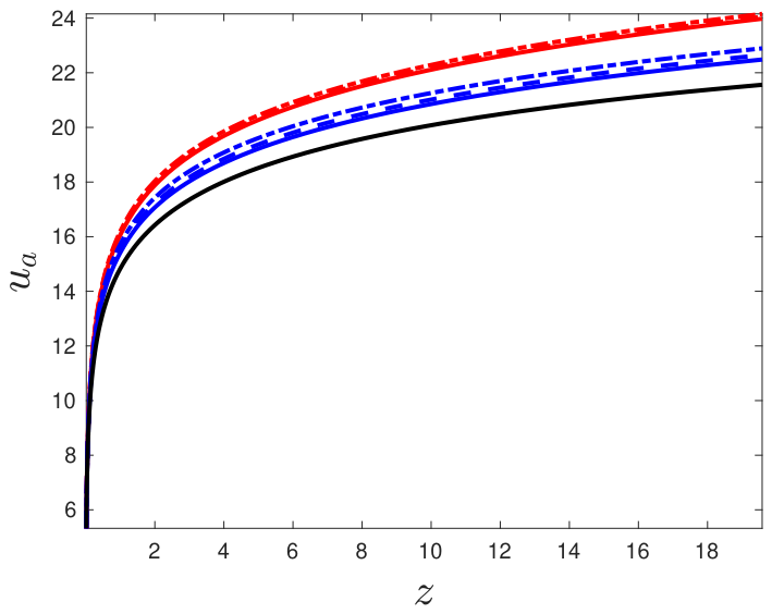
Figure 1 displays the vertical wind profiles and demonstrates that fine spray causes larger wind acceleration. This behavior is defined by two competing mechanisms, the spray-induced turbulence attenuation and the droplet inertia, the relative contributions of which depend on the droplet size. Small droplets attain higher volumetric concentrations s ( z ) above the wave crest for a fixed spray source intensity s 0 , resulting in more efficient turbulence suppression and, consequently, greater wind acceleration than that produced by large droplets. In contrast, large droplets exert a stronger decelerating effect at fixed s 0 since the inertial spray deceleration scales with the spray generation rate (12) s 0 a 0 (see (14)). Therefore, it increases with the droplet terminal velocity a 0 and, consequently, with the droplet size. This also explains the greater sensitivity of the wind profile to the droplet injection velocity U for large droplets, as illustrated in the figure: the spacing between the blue curves (large droplets) corresponding to different values of U is noticeably larger than that between the red ones (small droplets).
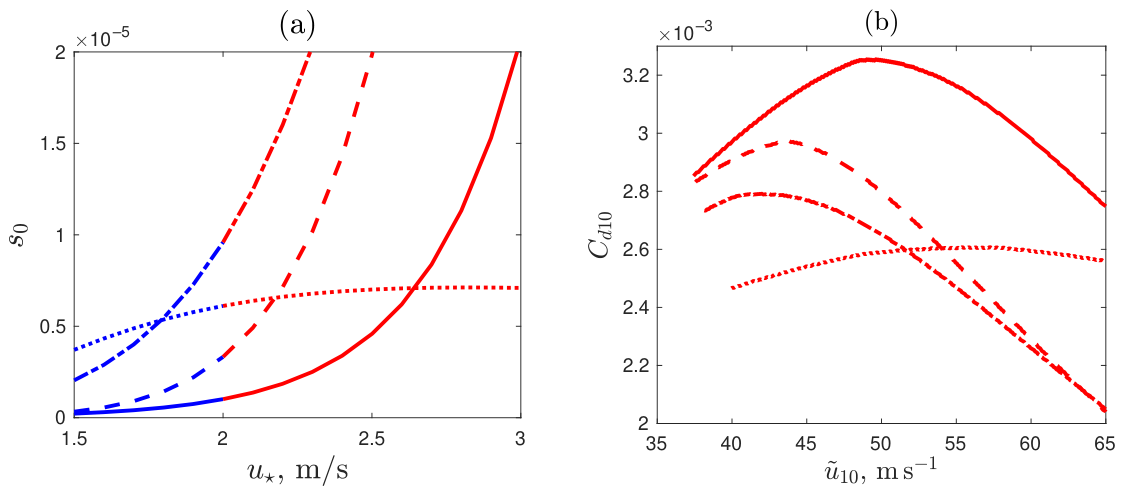
Spray production rates remain highly uncertain with figures found in the literature spanning up to six orders of magnitude even at relatively low wind speeds [25]. Although recent laboratory measurements have somewhat reduced this uncertainty [38,39,40], extrapolation of laboratory results to field conditions remains a nontrivial challenge for which no clear solution currently exists. To illustrate this, in Figure 2a we plot the correlations between the friction velocity and the expected sea spray concentration at the wave crest level suggested by various researchers. Namely, the solid line corresponds to exponential dependence suggested in [24,26]
s ˜ ( z w ) = A exp [ δ ( u 10 log u r ) ] , u 10 log = u k p ln 10 z ˜ 0 ,
where A = 2 × 10 7 , δ = 0.2 s m−1 and u r = 22 m s−1 [16]. The dashed and dash-dotted lines are given by
s ˜ ( z w ) = A n u n
with n = 5.37 , A 5.37 = 2.32 × 10 7 s5.37m−5.37 and n = 8 , A 8 = 1.3 × 10 8 s8m−8, respectively, estimated from the data presented in [25]. The dotted line is obtained by integrating the spray production number density function
s ˜ ( z ˜ w ) = 4 π 3 r min r max d F d r r 3 d r ,
where d F d r is given by equation (24) in [38], r min = 10 μ m and r max = 2500 μ m. All these distributions are based on field [24,25,26] or wind-tunnel [38] data collected at relatively low wind speeds (the blue segments of the curves) and are algebraically extrapolated to hurricane speed regimes (red segments). Not only do they produce very different numerical estimations, but they also exhibit completely different qualitative behaviors. The field data extrapolation suggests monotonic growth of spray concentration with the hurricane intensity, while the extrapolation of wind-tunnel data predicts that spray concentration reaches its maximum at about u = 3 m s−1 and then starts decreasing. The likely physical reason for such a discrepancy in extrapolations is that the first three correlations cited above are based on spume spray data (sea foam and white cap torn off wave crests and subsequently pulverized by the turbulent wind shear in the bulk of the air in open-sea conditions), while the last one considers the so-called bag-breakup mechanism driven by the shear at the air–water interface, which may dominate spray generation in wind-tunnel environments but is likely to become secondary in realistic hurricanes. We also note that wind-tunnel experiments indicate the dominant production of large droplets of up to a millimeter in diameter [38]. In hurricane conditions, turbulent shear in the bulk of air is likely to break such large droplets so that the effective droplet size reduces to 100–200 μ m [25], but that does not affect the total amount of spray estimated by expression (18), which is of interest in the context of this discussion. It is remarkable that despite these significant numerical and qualitative discrepancies in suggested extrapolations, the MABL models that we discuss here robustly and consistently predict similar qualitative behaviors of the main hurricane characteristics such as the drag coefficient as demonstrated in Figure 2b. Therefore, to keep this article at a reasonable length, in what follows we use the most conservative of the reviewed extrapolations of spume-based spray concentration function given by (16).
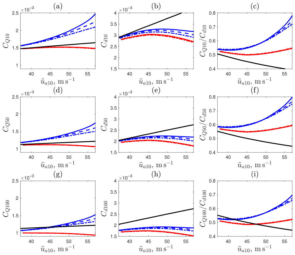
The dependence of the air–ocean drag coefficient C d , bulk total enthalpy transfer coefficient C Q , and their ratio C Q / C d (defined in Appendix C) on the wind speed u ˜ a 10 is presented in Figure 3 for the exponential law (16) for which the spray volumetric density at the wave crest level remains within physically reasonable limits and does not exceed 10 4 for the considered droplet radii at hurricane wind speeds u ˜ a 10 60 m s−1. Nevertheless, even much smaller spray volume fractions ∼10−5 lead to a noticeable decrease in the air–ocean drag coefficient relative to that in the reference spray-free atmosphere. A stronger reduction in the drag coefficient occurs for small droplets because, as discussed above, they suppress the air turbulence more efficiently producing a greater acceleration of the airflow. With an increasing wind speed, C d continues to increase, reaching a maximum at a certain spray volume fraction s max , the value of which depends sensitively on the droplet radius. Specifically, for droplets with r = 100 and 200 μ m, the calculations yield s max 2 × 10 5 and 4 × 10 5 , respectively. Such a behavior of the drag coefficient (reaching a maximum and then decreasing with wind speed) has indeed been observed in numerous field and laboratory measurements [28,41,42,43,44].
Figure 3b,e,h show that the behavior of the air–sea drag coefficient varies with altitude. In the reference spray-free atmosphere, the drag coefficients at 50 m ( C d 50 ) and 100 m ( C d 100 ) are very similar. However, in the spray-laden atmosphere, C d 100 becomes noticeably smaller than C d 50 for both large and small droplets (see the colored lines). This difference arises from the variable interplay between droplet inertia and turbulence suppression since these effects evolve differently with altitude. The influence of droplet inertia is largely confined to the near-surface region, where spray is injected into the MABL with a velocity much smaller than the local wind speed. As a result, the inertia-related contribution is nearly the same at higher altitudes of 50 and 100 m. In contrast, the TKE attenuation at a given altitude z ˜ is a result of the combined spray effects integrated from the surface up to that height. Thus, the degree of such suppression increases with altitude, leading to further reduction of the drag coefficient there. This means that the influence of spray on the turbulent flow cannot be adequately described by the drag coefficient evaluated at a single vertical position. This also implies that an accurate downward interpolation of field measurements of the drag coefficient from high altitudes at hurricane wind speeds is impossible without accounting for the spray influence on the wind velocity profile that deviates strongly from logarithmic existing in a spray-free atmosphere [28]. An attempt to do so may lead to an underestimation of the drag coefficient at medium amplitudes.

4. Thermodynamic Effect of Ocean Spray

The mechanical and thermodynamic effects of sea spray are interdependent: the spray-induced turbulence suppression reduces vertical heat and moisture fluxes while modifications of the vertical thermal and humidity stratifications in the boundary layer driven by air–droplet thermal exchange affect the TKE distribution, albeit to a much smaller degree. Because turbulence attenuation due to DS strongly influences the thermodynamic effect of spray, numerical results presented below are obtained using the multifluid model. The mixture model is employed in one explicitly noted instance to illustrate how the results change when the DS effect is neglected.
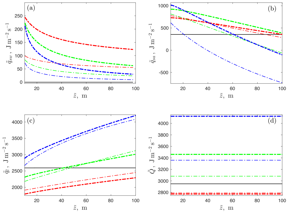
The vertical profiles of the sensible heat fluxes in the spray ( q ˜ s w ), in the air ( q ˜ s a ), along with the latent ( q ˜ l ) and total ( Q ˜ ) heat fluxes from the ocean to the atmosphere, are displayed in Figure 4. The figure shows that evaporating spray substantially redistributes the total heat flux between its latent and sensible components even when the volumetric spray concentration is small.
Figure 4c demonstrates that for a fixed value of s 0 , which determines the volumetric concentration ( s ˜ s 0 ) in the vicinity of the wave crest level, the latent heat flux q ˜ l increases with droplet size. This trend can be understood recollecting that the vertical latent heat flux is proportional to the specific humidity gradient and the intensity of turbulent transport. For fixed s 0 , the volumetric production of large droplets, s 0 a 0 , is greater than that of small droplets because their terminal velocity a 0 is larger. Furthermore, due to the gravitational pull, large droplets are mostly confined to a thin layer near wave crests. As a result of these combined effects, the evaporation of large droplets generates a noticeably steeper vertical moisture gradient than that of smaller ones. At the same time, large droplets induce weaker turbulence suppression resulting in stronger turbulent transport. Consequently, the combination of a sharper moisture gradient and more intensive turbulent transport noticeably enhances the latent heat flux for large droplets.
To examine how the latent heat flux q ˜ l varies with height z ˜ , we consider Equation (6) that yields the following expression for the latent heat flux q ˜ l :
q ˜ l ( z ˜ ) = q ˜ l ( z ˜ r ) z ˜ r z ˜ l ˜ s ˜ q ˙ ˜ d ξ ,
where z r is some reference point located above the wave crest level. Since the droplets evaporate ( q ˙ ˜ < 0 ), (19) implies that q ˜ l ( z ˜ ) increases monotonically with altitude z ˜ as corroborated by Figure 4c. As shown in Figure 4a, the sensible heat flux q ˜ s w ( z ˜ ) of water decreases at a slower rate with altitude for small droplets due to their larger concentrations at high altitudes compared to large droplets because turbulent eddies transports small droplets upwards more efficiently. Note that q ˜ s w constitutes a non-negligible portion of the total heat flux especially near the ocean surface. Neglecting it can lead to a significant under-prediction of the total heat flux.
With no internal heat sources above the wave crest level, the total enthalpy flux Q ˜ = q ˜ l + q ˜ s w + q ˜ s a remains constant throughout the domain as seen from Figure 4d, implying that evaporating droplets effectively convert the internal enthalpy of air into latent heat. Consequently, because q ˜ l increases with z ˜ , the total sensible heat flux q ˜ s w + q ˜ s a must decrease, and since q ˜ s a dominates q ˜ s w , it is also expected to decrease as indeed corroborated by Figure 4b.
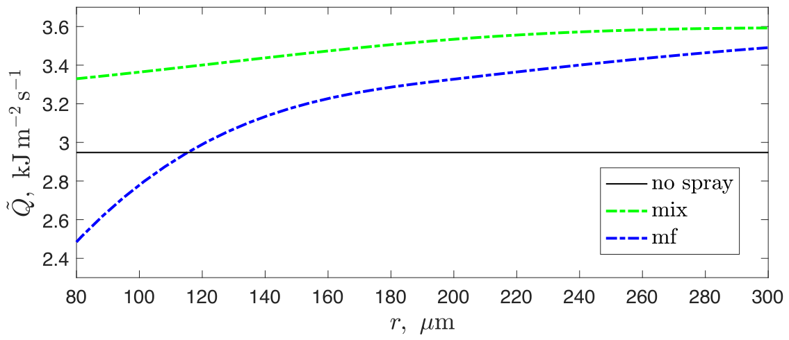
Figure 5 shows that when the spray production rate s 0 a 0 rather than the spray source intensity s 0 , which has been used as the control parameter thus far, is held constant, the dependence of the total heat flux Q ˜ on the droplet radius r is weak whenever the turbulence attenuation is negligible. Such a behavior is predicted by the mixture model because it does not account for the DS effect and the GL attenuation, which it does include, remains weak for low volumetric spray concentrations s 10 4 considered here. Consequently, for a fixed s 0 , Q ˜ predicted by the mixture model increases proportionally to a 0 , that is, approximately proportionally to the droplet size r. In contrast, the multifluid model accounting for the DS effect and predicting a strong turbulence attenuation and the associated decrease of the heat transport due to it reveal a much stronger pronounced nonlinear heat flux dependence on the droplet size shown by the blue line. Since the DS-induced attenuation of the turbulence intensity and transport is stronger for small droplets, the decrease in the total heat flux for droplets with ≲150 μm resulting from the multifluid model is much quicker than that shown by its mixture counterpart.
Figure 3a,d,g further show that the behavior of the bulk total enthalpy transfer coefficient C Q also depends on the droplet size. For small droplets with radius r = 100 μ m, C Q increases with wind speed, reaches a maximum at u ˜ a 10 45–50 m s−1 for the considered correlation laws, and then decreases. For all considered wind speeds and elevations, C Q remains below that sown by the black line and corresponding to the reference spray-free atmosphere. For large droplets r 200 μ m, a distinctly different behavior is observed with C Q increasing monotonically with wind speed. The cumulative effect of the spray-induced turbulence attenuation, integrated from the surface up to a given height, becomes stronger with increasing elevation. Consequently, at higher levels z ˜ = 100 m (panel (g)) it results in lower C Q than that at z ˜ = 50 m (panel (d)), even though the C Q values in the spray-free atmosphere remain close.
Figure 3c,f,i shows that for a reference spray-free atmosphere the ratio C Q / C d of the enthalpy exchange and air–sea drag coefficients decreases monotonically with increasing wind speed reaching approximately 0.4 for wind speed of 55 m s−1 at z ˜ = 10 m, with slightly larger values at higher elevations. These theoretical estimates for C Q / C d are obtained by extrapolating parameterizations derived at lower wind speeds. In contrast, the presence of sea spray causes the ratio to increase with wind speed reaching values of approximately 0.6 and 0.8 for small and large droplets, respectively. This is consistent with the observational evidence indicating that C Q 10 / C d 10 approaches 0.7 for tropical-storm wind speeds [42,45]. Therefore, our numerical simulations indicate that the inclusion of sea spray yields values that match closely the field data supporting the hypothesis that ocean spray is responsible for the observed increase in the C Q / C d ratio at high wind speeds.

5. Conclusions

This study focuses on modeling a turbulent, marine atmospheric boundary layer laden with evaporating ocean spray using an Eulerian multifluid and mixture approaches coupled with the E ϵ turbulence closure. The multifluid framework treats air and spray as interpenetrating continuous phases, providing a more detailed and physically consistent description than its mixture counterpart, which considers a single-phase system. It captures essential air–droplet interactions governing momentum transport, enthalpy exchange, and turbulence dynamics, enabling a consistent representation of spray-mediated heat and momentum exchange in the hurricane boundary layer. The mixture approach reduces complexity by treating the multi-phase system as a single medium with variable properties. Although it cannot adequately describe some important phase interactions, it is able to accurately capture the averaged characteristics of multi-phase flows. Its main advantage is simplicity: fewer governing equations facilitate numerical analysis and often enable the development of analytical solutions and reliable quantitative estimates characterizing underlying physical processes.
Spray influences the hurricane boundary layer through both mechanical and thermodynamic effects. The mechanical contribution comprises two competing effects: deceleration due to spray inertia and acceleration resulting from spray-induced turbulence attenuation, driven by two mechanisms—DS and GL associated with air–droplet friction and the loss of turbulent energy as eddies lift spray droplets, respectively. In this paper, we presented an analytical description of spray inertia and GL effects. The latter is modeled within a simplified mixture framework and our analysis shows that the deceleration associated with spray inertia overpowers the acceleration due to the GL effect. We also show numerically that the DS effect, which can be consistently described only within a more complex multifluid framework, overcomes the influence of droplet inertia and leads to wind acceleration for typical droplets with radii smaller than 200 μ m. This results in a reduction of the drag coefficient at hurricane wind speeds detected in field observations. Furthermore, spray induces a vertical variation of the drag coefficient that is primarily driven by the altitude-dependent suppression of turbulence while the effect of droplet inertia remains mostly confined to the near-surface region. Therefore, single-height estimates of the drag coefficient sometimes referred to in the literature are insufficient, and neglecting spray effects can lead to underestimation of drag when extrapolating field measurements downward.
Sea spray induces a coupled thermodynamic–mechanical influence on the hurricane boundary layer by redistributing the total heat flux between its latent and sensible components. Even in small amounts, evaporating droplets significantly increase the latent share of the total heat flux and reduce the sensible portion. The effect depends strongly on droplet size: small droplets suppress turbulence over a thicker layer and reduce both latent and total heat transport, whereas the influence of large droplets is confined to a near-surface region and enhances latent and total heat fluxes there. Our simulations show that sea spray reverses the decline in the ratio of the bulk total enthalpy and air–sea drag coefficients when the wind speed increases, yielding values consistent with field observations and indicating that spray is mostly responsible for the increase in this ratio at high wind speeds.


Author Contributions

Conceptualization, Y.R.; methodology, Y.R. and S.A.S.; numerical code development S.A.S., W.D. and Y.R., formal analysis, Y.R. and S.A.S.; writing—original draft preparation, Y.R. and S.A.S.; writing—review and editing, Y.R. and S.A.S.; supervision, Y.R.; project administration, Y.R.; funding acquisition, Y.R. and S.A.S. All authors have read and agreed to the published version of the manuscript.

Funding

This research was funded by the US National Science Foundation grant number 2302221.

Institutional Review Board Statement

Not applicable.

Informed Consent Statement

Not applicable.

Data Availability Statement

The original contributions presented in this study are included in the article material. Further inquiries can be directed to the corresponding author.

Conflicts of Interest

The authors declare no conflicts of interest.

Abbreviations

The following abbreviations are used in this manuscript:
DSDroplet Slip
GLGravity Lubrication
MABLMarine Atmospheric Boundary Layer
mfMultifluid Model
mixMixture Model
TKETurbulent Kinetic Energy

Appendix A. Estimation of the Spray Inertia Effect (Multifluid Model)

The dimensional momentum equation for a spray-laden flow is obtained by adding the dimensional versions of (1) and (2)
d d z ˜ ρ ˜ a k ˜ a d u ˜ a d z ˜ + ρ w k ˜ w s ˜ d u ˜ w d z ˜ + ρ w a 0 s 0 H ˜ z ˜ z w ( u ˜ w U ) = 0 .
Integrating (A1) with respect to the vertical coordinate z ˜ yields
ρ ˜ a k ˜ a d u ˜ a d z ˜ + ρ w k ˜ w s ˜ d u ˜ w d z ˜ + ρ w a 0 s 0 H ˜ z ˜ z w ( u ˜ w U ) = ρ a u 2 .
Upon nondimensionalizing (A2), we obtain
ρ a k a d u a d z + σ k w s 0 s d u w d z + σ a 0 s 0 u H z 1 ( u w U ) = 1 ,
where σ is the ratio of the water density ρ w and the dry air density at the ocean surface, ρ d 0 = P 0 / ( R d T 0 ) , and R d is the specific gas constant for dry air. Following the mixture assumptions (13) and neglecting turbulence attenuation by spray (setting k a = k p z ) reduce (A3) to
k p z ( ρ a + σ s s 0 ) d u a d z + σ a 0 s 0 u H z 1 ( u a U ) = 1 .
Below the wave crest level at z < 1 , H z 1 = 1 , s 1 and ρ a 1 . Hence, (A4) takes the form
k p 1 z d u a d z + k 1 ( u a U ) = 1 ,
where k p 1 = k p ( 1 + σ s 0 ) and k 1 = σ a 0 s 0 / u . The solution of this equation, subject to the boundary condition u a ( z 0 ) = 0 , takes the form
u a = 1 k 1 1 + k 1 U 1 z z 0 k 2 ,
where k 2 = k 1 / k p 1 . For low volumetric concentrations of spray σ s 0 1 , the following asymptotic expression is valid:
z z 0 k 2 = exp k 2 ln z z 0 1 k 2 ln z z 0 + 1 2 k 2 2 ln 2 z z 0 .
Substitution of (A7) into (A6) yields an approximate expression for u a :
u a 1 + k 1 U 1 + σ s 0 1 1 2 k 2 ln z z 0 1 k p ln z z 0 .
Upon expanding (A8) in σ s 0 and retaining only the first-order terms, we obtain
u a 1 k p ln z z 0 + k 1 U 1 2 k p ln z z 0 σ s 0 1 k p ln z z 0 .
The second term in (A9) quantifies the change in the wind speed due to spray inertia. At the wave crest level z = 1 it is
Δ u a 1 = k 1 U 1 2 k p ln 1 z 0 σ s 0 1 k p ln 1 z 0 ,
The two decelerating mechanisms associated with spray inertia can be distinguished in (A10). The first arises from the transfer of air momentum to sea spray droplets that are torn off the wave crests and are subsequently accelerated. This contribution is represented by the first term in the curly brackets. The second mechanism is due to higher spray concentration near the ocean surface, which increases the mass density of the air–spray mixture and reduces the local wind speed relative to the reference logarithmic profile. This contribution is given by the second term in the curly brackets in (A10).

Appendix B. Gravity Lubrication (Mixture Model)

Asymptotic Solution for Small Spray Concentration

Since the vertical droplet motion on which the gravity lubrication effect depends is consistently captured by the mixture model, this effect can be adequately described within this framework. As derived in [23] for small spray concentration, that is, for 0 < π 12 1 , the leading order approximation to distributions of spray concentration s, TKE e, dissipation rate ϵ a of TKE and the wind speed u a can be found in the form of an asymptotic expansion
s = z λ + λ π 12 s 1 + , e a = 1 α + λ π 12 e a 1 + , ϵ a = 1 k p z + λ π 12 ϵ a 1 + , u a = u a ( 1 ) + 1 k p ln z + λ π 12 u a 1 + ,
where π 12 plays the role of an asymptotic expansion parameter. At the order ( π 12 ) 1 we obtain
s 1 = k p λ z λ u a 1 , e a 1 = A 1 z τ z 1 λ , ϵ a 1 = A 4 z 2 z λ 2 λ + A 5 z 1 τ z 2 , u a 1 = ( A 7 A 4 ) z 1 λ 1 1 λ + A 4 z 1 λ z 1 2 λ + A 5 z 1 1 + A 6 z τ 1 ,
where Prandtl constant k p = 0.43 , τ = 1.79 , λ = π 1 k p and
A 1 = 1 α e ( τ 2 ( 1 λ ) 2 ) , A 2 = α A 1 α ϵ k p 3 2 α C ϵ , 1 α ϵ k p 2 ( 3 + 2 τ ) , A 3 = α C ϵ , 1 α ϵ k p α A 1 α ϵ k p 3 2 α C ϵ , 1 α ϵ k p 2 ( 1 + 2 λ ) , A 4 = A 3 λ + 1 , A 5 = A 2 ( τ + 2 ) ( τ 1 ) , A 6 = 2 α A 1 k p A 5 k p τ , A 7 = 2 α A 1 k p .
For λ = 1 + δ , δ 1 neglecting terms quadratic in π 12 and δ we have
s = z 1 ( 1 + δ ln z ) k p π 12 z 1 ( A 4 A 5 ) 1 z 1 + A 6 z τ 1 + ( A 7 A 4 ) ln z + , e a = 1 α + π 12 A 1 z τ 1 + , ϵ a = 1 k p z + π 12 A 4 z 2 z 1 + A 5 z 1 τ z 2 + , u a = u a ( 1 ) + 1 k p ln z + π 12 ( A 4 A 5 ) 1 z 1 + A 6 z τ 1 + ( A 7 A 4 ) ln z + , A 1 0.31 , A 4 0.32 , A 5 0.04 , A 6 0.26 , A 7 0.43 .
In the double limit of low spray concentration ( π 12 1 ) and small droplets ( λ 1 ) the corresponding expressions become
s = 1 λ ln z + λ 2 2 ln 2 z + , e a = 1 α + λ π 12 A 1 z τ z + , ϵ a = 1 k p z + λ π 12 A 4 z 2 1 2 + A 5 z 1 τ z 2 + , u a = u a ( 1 ) + 1 k p ln z + λ π 12 A 4 1 z + z 1 2 + A 5 z 1 1 + A 6 z τ 1 + A 7 ( z 1 ) + , A 1 0.45 , A 4 0.27 , A 5 0.06 , A 6 0.38 , A 7 0.63 .
The typical distribution of the ratio
R = π 13 λ u a 1 π 1 u a 1 2 u a ( 1 ) 1 u a ( 1 )
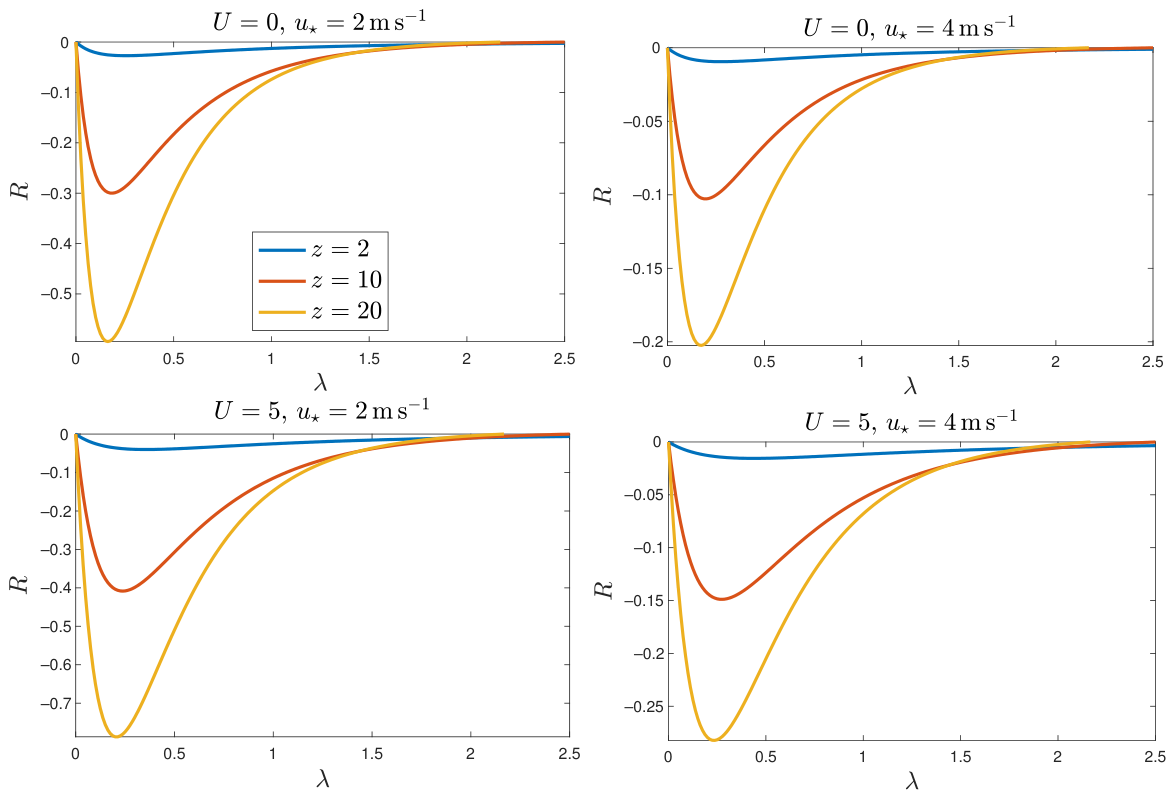
of the wind speed increase due to the gravitational lubrication to its deceleration due to spray inertia is shown in Figure A1. It demonstrates that spray inertia always dominates over GL for the expected values of π 12 1 (small spray concentration).
Figure A1. The ratio of the gravitational lubrication and inertia effects given by Equation (A11).
Atmosphere 17 00559 g0a1

Appendix C. Heat Fluxes and Bulk Transfer Coefficients

Above the wave crest level, the dimensional latent heat flux q ˜ l , the sensible heat fluxes in the air and spray, q ˜ s a and q ˜ s w , respectively, and the total heat flux Q ˜ can be written as
q ˜ l = α v l k ˜ a ρ ˜ a d q ˜ d z ˜ , q ˜ s a = α T c p d k ˜ a f a ρ ˜ a d θ ˜ d z ˜ , q ˜ s w = c w d ˜ w ρ w s ˜ d T ˜ w d z ˜ , Q ˜ = q ˜ l + q ˜ s a + q ˜ s w ,
where c p d , c w , and l are the dimensional specific heat capacities of air and liquid water, and the latent heat of evaporation, respectively, and α v = α T = 1 . The expression for the air–ocean drag coefficient C d and bulk total enthalpy coefficients are given by
C d = τ 0 ρ ˜ a u ˜ a 2 + ρ ˜ w s ˜ u ˜ w 2 u ˜ w 0 2 , C Q = Q ˜ ρ ˜ a u ˜ a l q 0 1 π 9 q ˜ + c p d f a ρ ˜ a u ˜ a ( T 0 θ ˜ ) + c w ρ w s ˜ u ˜ w T ˜ 0 w T ˜ w ,
where τ 0 is a constant turbulent shear stress above the wave crest level, and u ˜ w 0 and T ˜ 0 w are the average horizontal velocity and temperature of spray at z ˜ = z ˜ 0 , respectively.

Appendix D. Definitions of the δ z and H z Functions

The present formulation employs the localized δ z and the integral function H z [46] defined as
δ z = π 0 2 [ 1 + cos ( π π 0 z ) ] , | π 0 z | 1 , 0 , | π 0 z | > 1 , H z = 1 , π 0 z < 1 , π ( 1 π 0 z ) sin ( π π 0 z ) 2 π , | π 0 z | 1 , 0 , π 0 z > 1 .
In the reported computations, the nondimensional inverse thickness of the spray production layer was taken to be π 0 = z w 2 h = 2.5 .

References

  1. Zhang, L.; Zhang, X.; Perrie, W.; Guan, C.; Dan, B.; Sun, C.; Wu, X.; Liu, K.; Li, D. Impact of Sea Spray and Sea Surface Roughness on the Upper Ocean Response to Super Typhoon Haitang (2005). J. Phys. Ocean. 2021, 51, 1929–1945. [Google Scholar] [CrossRef]
  2. Bruch, W.; Yohia, C.; Tulet, P.; Limoges, A.; Sutherland, P.; van Eijk, A.M.J.; Missamou, T.; Piazzola, J. Atmospheric Sea Spray Modeling in the North-East Atlantic Ocean using Tunnel-Derived Generation Functions and the SUMOS Cruise Data Set. J. Geophys. Res. D Atmos. 2023, 128, e2022JD038330. [Google Scholar] [CrossRef]
  3. Richter, D.H.; Wainwright, C.E. Large-Eddy Simulation of Sea Spray Impacts on Fluxes in the High-Wind Boundary Layer. Geophys. Res. Lett. 2023, 50, e2022GL101862. [Google Scholar] [CrossRef]
  4. Lin, T.; Spengler, T.; Rutgersson, A.; Wu, L. Impact of sea spray-mediated heat fluxes on polar low development. Q. J. R. Meteorol. Soc. 2024, 150, 2976–2990. [Google Scholar] [CrossRef]
  5. Rastigejev, Y.; Suslov, S.A. Polydisperse Sea Spray Effect on the Vertical Momentum Transport in Hurricanes. J. Atmos. Sci. 2024, 81, 1127–1146. [Google Scholar] [CrossRef]
  6. Barr, B.W.; Chen, S.S. Impacts of Seastate-Dependent Sea Spray Heat Fluxes on Tropical Cyclone Structure and Intensity in Fully Coupled Atmosphere-Wave-Ocean Model Simulations. J. Adv. Model. Earth Syst. 2025, 17, e2024MS004550. [Google Scholar] [CrossRef]
  7. Rastigejev, Y.; Suslov, S.A. Modeling sea spray influence on vertical enthalpy and momentum transport in hurricanes with the multifluid approach. J. Atmos. Sci. 2026, 83, 589–614. [Google Scholar] [CrossRef]
  8. Manninen, M.; Taivassalo, V.; Kallio, S. On the Mixture Model for Multiphase Flow; VTT Publications; Technical Research Centre of Finland: Espoo, Finland, 1996; Volume 288. [Google Scholar]
  9. Massot, M. Eulerian Multi-Fluid Models for Polydisperse Evaporating Sprays; Springer: Vienna, Austria, 2007. [Google Scholar]
  10. Jakobsen, H.A. Chemical Reactor Modeling: Multiphase Reactive Flows; Springer: Berlin/Heidelberg, Germany, 2008. [Google Scholar]
  11. Sommerfeld, M. Numerical Methods for Dispersed Multiphase Flows. In Particles in Flows; Springer International Publishing: Cham, Switzerland, 2017; pp. 327–396. [Google Scholar]
  12. Vikhansky, A. Modelling of high-velocity free-surface flows: A revised interfacial area approach. J. Hydraul. Res. 2024, 62, 477–487. [Google Scholar] [CrossRef]
  13. Barenblatt, G.I.; Chorin, A.J.; Prostokishin, V.M. A note concerning the Lighthill “sandwich model” of tropical cyclones. Proc. Natl. Acad. Sci. USA 2005, 102, 1115–1148. [Google Scholar] [CrossRef]
  14. Kudryavtsev, V.N. On the effect of sea drops on the atmospheric boundary layer. J. Geophys. Res. 2006, 111, C07020. [Google Scholar] [CrossRef]
  15. Rastigejev, Y.; Suslov, S.A.; Lin, Y.L. Effect of ocean spray on vertical momentum transport under high-wind conditions. Bound. Layer Meteorol. 2011, 141, 1–20. [Google Scholar] [CrossRef]
  16. Rastigejev, Y.; Suslov, S.A. Investigation of Sea Spray Effect on the Vertical Momentum Transport Using an Eulerian Multifluid-Type Model. J. Phys. Ocean. 2022, 52, 99–117. [Google Scholar] [CrossRef]
  17. Crowe, C.T.; Schwarzkopf, J.D.; Sommerfeld, M.; Tsuji, Y. Multiphase Flows with Droplets and Particles, 2nd ed.; Taylor & Francis: Boca Raton, FL, USA, 2011. [Google Scholar]
  18. Simonin, O. Prediction of the dispersed phase turbulence in particle-laden jets. In Proceedings of the Fourth International Symposium On Gas-Solid Flows, ASME FED, Portland, OR, USA, 23–27 June 1991; Volume 121, pp. 197–206. [Google Scholar]
  19. Launder, B.E.; Spalding, D.B. The numerical computation of turbulent flows. Comput. Methods Appl. Mech. Eng. 1974, 3, 269–289. [Google Scholar] [CrossRef]
  20. Rastigejev, Y.; Suslov, S.A. Two-temperature non-equilibrium model of a marine boundary layer laden with evaporating ocean spray under high-wind conditions. J. Phys. Ocean. 2016, 46, 3083–3102. [Google Scholar] [CrossRef]
  21. Stull, R.B. An Introduction to Boundary Layer Meteorology; Atmospheric and Oceanographic Sciences Library; Springer: Dordrecht, The Netherlands, 1988. [Google Scholar]
  22. Simonin, O.; Viollet, P.L. Prediction of an oxygen droplets pulverization in a compressible subsonic coflowing hydrogen flow. In Numerical Methods for Multiphase Flows; ASME FED: New York, NY, USA, 1990; Volume 91, pp. 73–82. [Google Scholar]
  23. Rastigejev, Y.; Suslov, S.A. E-ϵ model of spray-laden near-sea atmospheric layer in high wind conditions. J. Phys. Ocean. 2014, 44, 742–763. [Google Scholar] [CrossRef]
  24. Wu, J. Production of spume drops by the wind tearing of wave crests: The search for quantification. J. Geophys. Res. 1993, 98, 18221–18227. [Google Scholar] [CrossRef]
  25. Andreas, E.L. A new sea spray generation function for wind speeds up to 32 m/s. J. Phys. Oceanogr. 1998, 28, 2175–2184. [Google Scholar] [CrossRef]
  26. Monahan, E.C. The ocean as a source for atmospheric particles. In The Role of Air-Sea Exchange in Geochemical Cycling; Springer: Dordrecht, The Netherlands, 1986; pp. 129–163. [Google Scholar]
  27. Rastigejev, Y.; Suslov, S.A. Effect of Evaporating Sea Spray on Heat Fluxes in a Marine Atmospheric Boundary Layer. J. Phys. Ocean. 2019, 49, 1927–1948. [Google Scholar] [CrossRef]
  28. Powell, M.D.; Vickery, P.J.; Reinhold, T.A. Reduced drag coefficient for high wind speeds in tropical cyclones. Nature 2003, 422, 279–283. [Google Scholar] [CrossRef]
  29. Jarosz, E.; Mitchell, D.A.; Wang, D.W.; Teague, W.J. Bottom-up determination of air-sea momentum exchange under a major tropical cyclone. Science 2007, 315, 1707–1709. [Google Scholar] [CrossRef] [PubMed]
  30. Holthuijsen, L.H.; Powell, M.D.; Pietrzak, J.D. Wind and waves in extreme hurricanes. J. Geophys. Res. 2012, 117, C09003. [Google Scholar] [CrossRef]
  31. Crowe, C.T. Multiphase Flow Handbook; Taylor & Francis: Boca Raton, FL, USA, 2005. [Google Scholar]
  32. Gore, R.A.; Crowe, C.T. Effect of particle size on modulating turbulent intensity. Int. J. Multiph. Flow 1989, 15, 279–285. [Google Scholar] [CrossRef]
  33. Elghobashi, S.E.; Abou-Arab, T. A two-equation turbulence model for two-phase flows. Phys. Fluids. 1983, 26, 931––938. [Google Scholar] [CrossRef]
  34. Subramaniam, S.; Balachandar, S. (Eds.) Modeling Approaches and Computational Methods for Particle-Laden Turbulent Flows; Academic Press: London, UK, 2023. [Google Scholar]
  35. Simonin, O. Continuum modelling of dispersed two-phase flows. Lect. Ser.—Von Karman Inst. Fluid Dyn. 1996, 2, K1–K47. [Google Scholar]
  36. Kulick, J.D.; Fessler, J.R.; Eaton, J.K. Particle response and turbulence modification in fully developed channel flow. J. Fluid Mech. 1994, 277, 109––134. [Google Scholar] [CrossRef]
  37. Sahu, S.; Hardalupas, Y.; Taylor, A.M.K.P. Droplet–turbulence interaction in a confined polydispersed spray: Effect of turbulence on droplet dispersion. J. Fluid Mech. 2016, 794, 267–309. [Google Scholar] [CrossRef]
  38. Troitskaya, Y.; Kandaurov, A.; Ermakova, O.; Kozlov, D.; Sergeev, D.; Zilitinkevich, S. The “Bag Breakup” Spume Droplet Generation Mechanism at High Winds. Part I: Spray Generation Function. J. Phys. Ocean. 2018, 48, 2167–2188. [Google Scholar] [CrossRef]
  39. Fairall, C.W.; Banner, M.L.; Peirson, W.L.; Asher, W.; Morison, R.P. Investigation of the physical scaling of sea spray spume droplet production. J. Geophys. Res. 2009, 114, 1–19. [Google Scholar] [CrossRef]
  40. Ortiz-Suslow, D.G.; Haus, B.K.; Mehta, S.; Laxague, N.J.M. Sea Spray Generation in Very High Winds. J. Atmos. Sci. 2016, 73, 3975–3995. [Google Scholar] [CrossRef]
  41. Donelan, M.A.; Haus, B.K.; Reul, N.; Plant, W.J.; Stiassnie, M.; Graber, H.C.; Brown, O.B.; Saltzman, E.S. On the limiting aerodynamic roughness of the ocean in very strong winds. Geophys. Res. Lett. 2004, 31, L18306. [Google Scholar] [CrossRef]
  42. Black, P.G.; D’Asoro, E.A.; Drennan, W.M.; French, J.R.; Niller, P.P.; Sanford, T.B.; Terril, E.J.; Walsh, E.J.; Zhang, J.A. Air–sea exchange in hurricanes. Synthesis of observations from the coupled boundary layer air–sea transfer experiment. Bull. Am. Meteorol. Soc. 2007, 88, 357–374. [Google Scholar] [CrossRef]
  43. Zhao, D.; Li, M. Dependence of wind stress across an air—Sea interface on wave states. J. Oceanogr. 2019, 75, 207–223. [Google Scholar] [CrossRef]
  44. Sun, D.; Song, J.; Li, X.; Ren, K.; Leng, H. A Novel Sea Surface Roughness Parameterization Based on Wave State and Sea Foam. J. Mar. Sci. Eng. 2021, 9, 246. [Google Scholar] [CrossRef]
  45. French, J.R.; Drennan, W.M.; Zhang, J.A.; Black, P.B. Turbulent fluxes in the hurricane boundary layer. Part I: Momentum fluxes. J. Atmos. Sci. 2007, 64, 1089–1102. [Google Scholar] [CrossRef]
  46. Peskin, C.S. Numerical analysis of blood flow in the heart. J. Comp. Phys. 1977, 25, 220–252. [Google Scholar] [CrossRef]
Figure 1. Wind profiles for s 0 = 2 × 10 5 , T 0 = 300 K, P 0 = 101.3 kPa, u = 3 m s−1, θ = 0.1 K, and q = 3 × 10 4 . The red and blue lines correspond to droplet radii r = 100 and 200 μ m, respectively. The solid, dashed and dash-dotted lines correspond to the non-dimensional droplet injection speed U = 0, 2 and 5, respectively. The black line shows the wind velocity profile in a reference spray-free atmosphere.
Atmosphere 17 00559 g001
Figure 2. (a) The dependence of spray concentration on friction velocity suggested in [24,26] (solid line), Ref. [25] (dashed and dash-dotted lines) and [38] (dotted line). The u range for which either field or experimental data are available is shown in blue, the algebraic extrapolations are given in red. (b) Model predictions of the drag coefficient at 10 m above the average sea level based on the extrapolated spray correlations shown in panel (a).
Atmosphere 17 00559 g002
Figure 3. Coefficients C Q and C d and their ratio for T 0 = 300 K, P 0 = 101.3 kPa, θ = 0.1 K, q = 3 × 10 4 and (ac) z ˜ = 10 , (df) 50 and (gi) 100 n s−1 above the mean sea level. The red and blue lines correspond to droplet radii r = 100 and 200 μ m, respectively. The solid, dashed and dash-dotted lines correspond to the droplet non-dimensional injection speed of U = 0 , 2 and 5, respectively. The black lines show the coefficient values in a reference spray-free atmosphere.
Atmosphere 17 00559 g003
Figure 4. Distributions of (a) sensible heat flux in the spray, (b) sensible heat flux in the air, (c) latent heat flux, and (d) total heat flux from the ocean to atmosphere in MABL for spray injection speed U = 0 . The red, green, and blue lines correspond to droplet radii r = 100 , 150 and 200 μ m, respectively. The thick and thin colored lines correspond to spray source intensities s 0 = 2 × 10 5 and 6 × 10 5 , respectively. The thin black solid lines correspond to a reference spray-free atmosphere. Parameter values of T 0 , P 0 , u and q are the same as in Figure 1.
Atmosphere 17 00559 g004
Figure 5. Total heat flux Q ˜ as a function of droplet radius. The horizontal black line represents the total heat flux in the reference spray-free atmosphere. The dotted green and blue lines correspond to the mixture and multifluid models, respectively. All data are shown for fixed spray production rate s 0 a 0 = 3 × 10 5 . The rest of the parameters are as in Figure 4.
Atmosphere 17 00559 g005
Table 1. The definitions and meaning of the main non-dimensional parameters entering the governing equations.
ParameterDefinitionMeaning
π 0 z w 2 h Inverse thickness of spray production layer
π 1 a 0 u Ratio of terminal droplet speed and friction velocity
π 2 3 D 0 q 0 z w r 2 σ u Ratio of droplet evaporation rate and turbulent diffusion
π 3 3 D 0 s 0 z w α v r 2 u Ratio of humidity change rates due to droplet evaporation and turbulent diffusion
π 5 3 K 0 s 0 z w α T r 2 u c p d ρ d 0 Ratio of air–droplet thermal exchange and turbulent sensible heat transfer rates in air
π 6 3 K 0 z w r 2 u c w ρ w Ratio of air–droplet thermal exchange and turbulent sensible heat transfer rates in liquid phase
π 7 3 D 0 q 0 z w l 0 r 2 c w σ u T 0 Ratio of latent heat release and sensible heat transfer rates in liquid phase
π 8 g z w R d T 0 Ratio of wave height and characteristic pressure variation scale
π 9 R v R d R d q 0 Characteristic specific humidity
π 12 g σ s 0 z w u 2 Ratio of turbulence destruction rate due to vertical spray stratification and turbulence production due to wind shear
π 13 α T g z w u 2 Ratio of turbulence production rate due to temperature variation and turbulence production due to wind shear
π 17 a 0 u g z w Ratio of air–droplet momentum exchange rate due to friction and turbulent transport of spray momentum
Disclaimer/Publisher’s Note: The statements, opinions and data contained in all publications are solely those of the individual author(s) and contributor(s) and not of MDPI and/or the editor(s). MDPI and/or the editor(s) disclaim responsibility for any injury to people or property resulting from any ideas, methods, instructions or products referred to in the content.