Article

Longwave Radiation Variability in the Arctic: Forty Years of Change Under Reducing Global Anthropogenic SO2 Emissions


1
Arctic and Antarctic Research Institute (AARI), 38 Bering Str., St. Petersburg 199397, Russia
2
Independent Researcher, Columbia, SC 29212, USA
*
Author to whom correspondence should be addressed.
Atmosphere 2026, 17(5), 513; https://doi.org/10.3390/atmos17050513
Submission received: 29 March 2026 / Revised: 12 May 2026 / Accepted: 15 May 2026 / Published: 18 May 2026
(This article belongs to the Section Meteorology)

Abstract

This study presents a comprehensive assessment of longwave radiation variability in the Arctic based on unique measurements collected at the North Pole drifting station SP-28 in 1987. The primary objective is to compare these historical observations with modern datasets from the Surface Heat Budget of the Arctic Ocean (SHEBA, 1997–1998) and the Multidisciplinary drifting Observatory for the Study of Arctic Climate (MOSAiC, 2019–2020) to evaluate long-term changes in the Arctic radiation regime. Continuous longwave radiation measurements were obtained using high-precision spectral pyrgeometers to identify Arctic haze. The results show that in 1987, Arctic haze layers enhanced the downward longwave flux by 15–20 W·m−2 and increased atmospheric emissivity. In contrast, MOSAiC observations reveal emissivity values that closely match aerosol-free model calculations, indicating a substantial decline in Arctic haze and the diminishment of radiatively significant aerosol layers. This shift is in alignment with the long-term reduction of global anthropogenic sulfur dioxide emissions across the Northern Hemisphere.

1. Introduction

Radiative heat transfer between the atmosphere and the surface is a fundamental component of the Earth’s energy balance and plays a central role in shaping the thermal structure of the lower troposphere. Even small variations in the concentration of radiatively active gases or aerosols can significantly modify longwave fluxes.
Although the Arctic atmosphere has traditionally been regarded as exceptionally clean, observations beginning in the mid-20th century revealed that substantial amounts of anthropogenic aerosol are transported into the region during winter and spring from mid-latitude industrial areas of Eurasia and North America [1,2]. These pollutants form a persistent Arctic haze which affects both shortwave and longwave radiative transfer. However, for many years the longwave radiative impact of this haze remained poorly quantified due to the lack of high-precision measurements.
Modern observations show that the radiation regime of the Arctic has undergone significant changes over the past 25–30 years. Data from SP-28 [3], SHEBA [4] and MOSAiC [5] serve as the observational basis for this study. The authors have obtained a unique long-term series demonstrating a gradual weakening of the aerosol effect on longwave radiation.
A clear visual manifestation of Arctic haze is shown in Figure 1, which illustrates its appearance and vertical structure under different observational conditions. These images, obtained by the author during flights near the North Pole, demonstrate the stratified nature of the aerosol layer and its persistence within strong surface inversions.
During flights conducted on 17–19 April 2001, photographs of the haze layer were obtained at altitudes of 350 m, 400 m, and 180 m, as well as from the surface of the sea ice. Panels (a)–(c) show the haze as observed from the aircraft at different heights, while panel (d) presents the view from the ice surface.
The first continuous longwave radiation measurements capable of resolving the radiative signature of Arctic haze were obtained at the drifting station SP-28 in 1987. These observations, covering several seasons, showed that aerosol condensation layers embedded within strong surface-based radiation inversions can substantially enhance the downward longwave flux and increase atmospheric emissivity (The term “atmospheric emissivity” is defined in Section 2.4).
Measurements in the late 1980s confirmed the magnitude of this effect, indicating that radiatively active aerosol layers were a persistent element of the Arctic atmosphere at that time. The physical mechanisms underlying this enhancement were consistent with earlier theoretical developments. Wexler [6] first described the formation of strong surface-based radiation inversions in polar air masses, while Curry [7] later showed that even small amounts of condensate within an inversion can dramatically increase longwave cooling efficiency. Additional studies in the 1980s and early 1990s [8,9] demonstrated that thin aerosol or condensation layers embedded within stable inversions can exert a disproportionately strong influence on longwave fluxes.
Over the past several decades, however, the Arctic radiation regime has undergone substantial changes. Reanalysis of SP-28 data, combined with newly processed observations from SHEBA and MOSAiC, reveals a systematic decline in the longwave aerosol effect. Modern emissivity values closely match calculations for an aerosol-free atmosphere, suggesting that radiatively significant Arctic haze has largely disappeared. This shift coincides with a long-term reduction in anthropogenic sulfur dioxide emissions across the Northern Hemisphere, which has led to a pronounced decrease in sulfate aerosols—the primary component of Arctic haze.
The aim of this study is to quantify the longwave radiative impact of Arctic haze using historical and modern datasets and to assess how the decline in anthropogenic sulfur emissions has altered the radiative properties of the Arctic atmosphere over the past four decades.

2. Materials and Methods

Experimental studies were carried out at the drifting station SP-28, which operated in the Central Arctic Basin from February to October 1987.

2.1. Mode and Experimental Setup

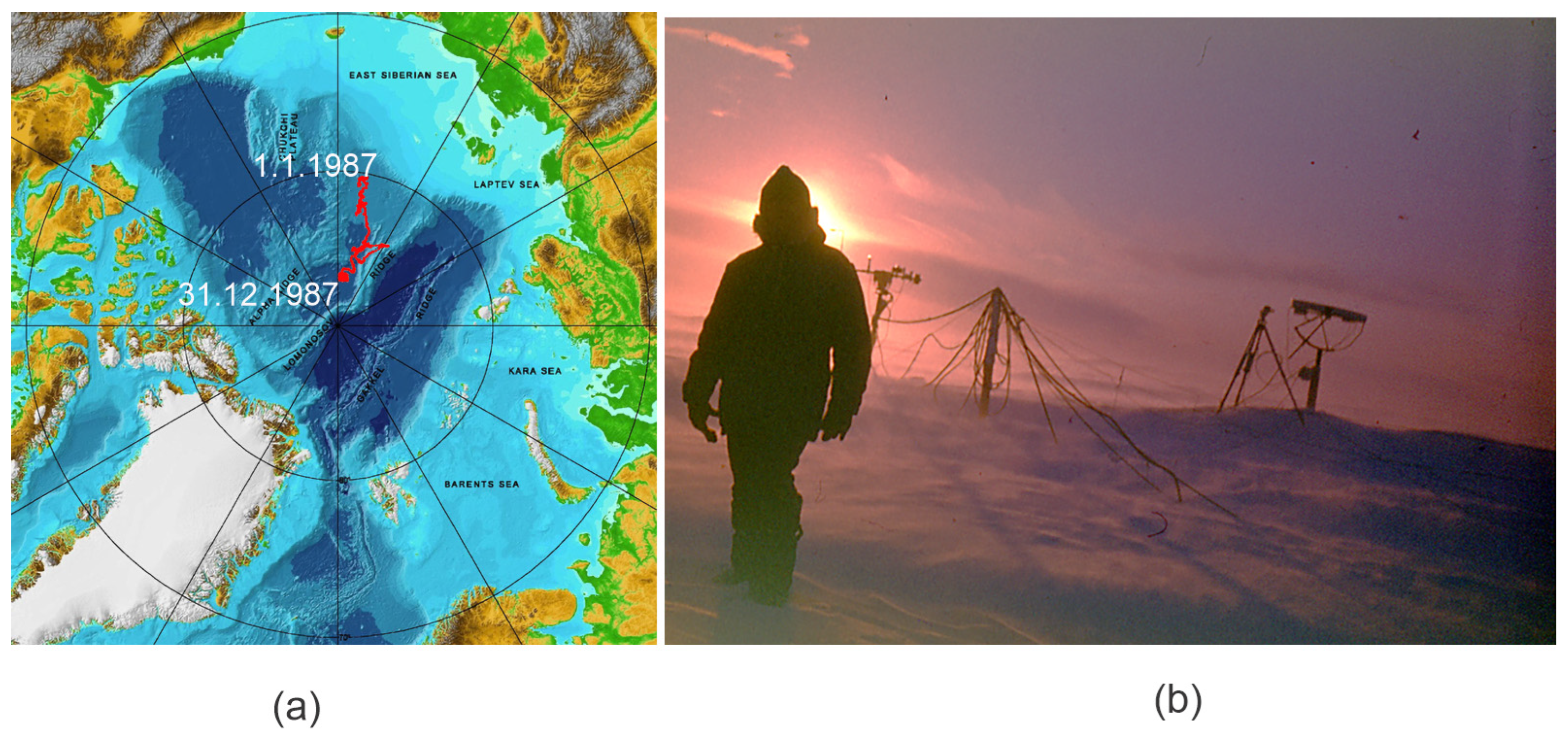
The drift area covered latitudes of 81–85° N and longitudes of 140–170° E, corresponding to one of the most remote and climatically stable regions of the Arctic. These conditions ensured minimal influence from local aerosol sources and allowed for the consideration of observed radiation characteristics as a reflection of large-scale transport and transformation processes of air masses.
The station was located on multiyear sea ice several meters thick, which provided a stable platform for the installation of radiation instruments as shown in Figure 2. The absence of open water in the drift zone eliminated the influence of local thermal anomalies and ensured the homogeneity of the underlying surface, which is an important condition for the correct interpretation of longwave measurements.
The spring season, particularly the transition from the polar night to the polar day, is of critical importance for the analysis of the seasonal evolution of atmospheric radiation parameters. During this period, anthropogenic SO2 accumulated in the Arctic atmosphere during the dark winter months begins to interact with incoming solar ultraviolet (UV) radiation. This photochemical process triggers the transformation of gaseous precursors into radiatively active sulfate aerosols, leading to the observed peak in Arctic haze and its subsequent impact on the longwave radiation field.
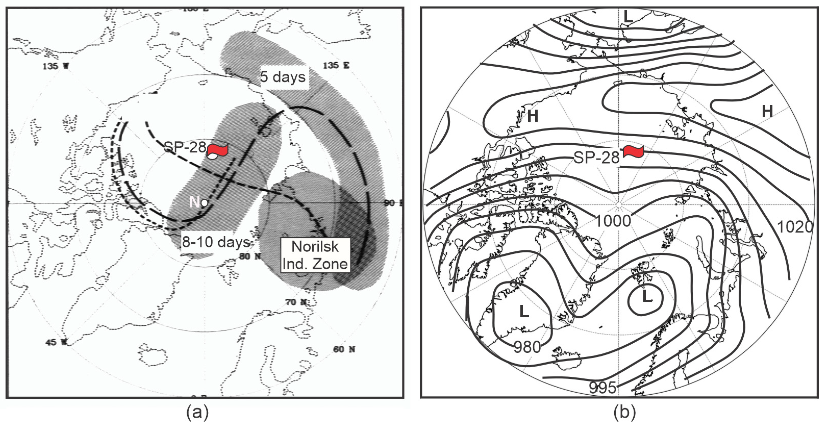
The synoptic situation in the Arctic in March 1987, as illustrated in Figure 3, created unique conditions for the study of the longwave radiation effects of aerosol.
The average monthly pressure in the drift area exceeded the climatological norm by 4–6 hPa, which indicated an abnormally strong Arctic anticyclone system. The air temperature in January–March was 2–7 °C below normal, and in April–June it was near to the average. Such conditions contributed to the formation of strong surface-based radiation inversion, which played a central role in retaining the Arctic haze and enhancing its longwave impact.
During the period from February 18 to April 4, the drift area was in the zone of interaction between North Atlantic cyclones and the eastern periphery of the Arctic anticyclone. During this period, the wind was mainly southwesterly, which created favorable conditions for the transfer of aerosol from the industrial regions of Siberia, including the Norilsk industrial area. These features are consistent with known seasonal patterns of impurity transport in the Siberian sector of the Arctic, described in international studies. From April 5 to June 24, a stable anticyclonic regime was established with easterly winds and pressure 4–6 hPa above normal. During this period, the strongest surface-based radiation inversion and the maximum probability of Arctic haze formation were observed.
Thus, the synoptic conditions of 1987 provided a favorable background for studying the Arctic haze longwave effects: sustained inversions, weak turbulence, lack of precipitation, and long periods of cloudless skies.

2.2. Radiometric Equipment

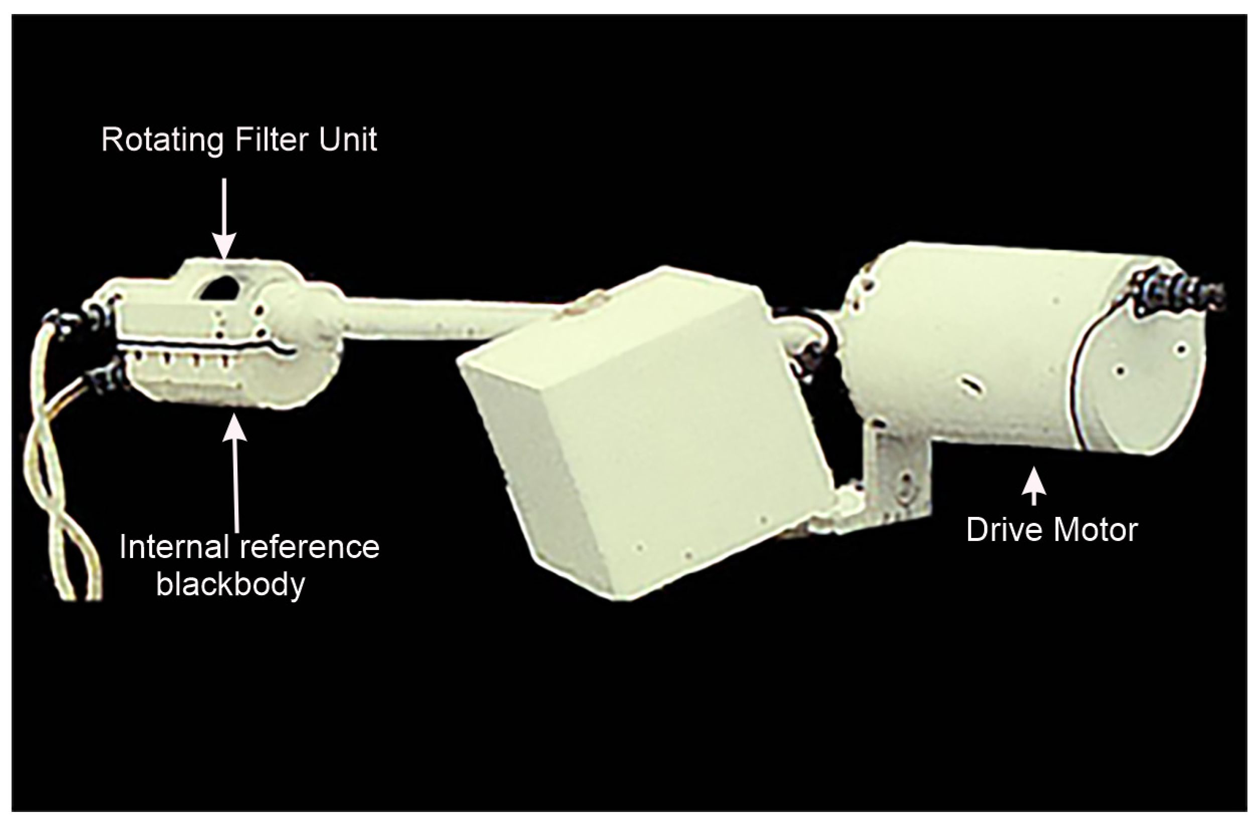
For precise measurements of downwelling longwave radiation, spectral pyrgeometers P2-30 (1.8–30 μm) and P8-12 (8–12 μm) were used, following the ideas laid down by Hinzpeter [10] and Paltridge [11]. These instruments, developed at the Arctic and Antarctic Research Institute (AARI) [12] through the deep modernization of the balance meter created at the Main Geophysical Observatory (MGO), are shown in Figure 4.
The devices are equipped with highly sensitive MTS-P thermoelectric receivers, built-in controllable hollow-cavity blackbody emitters, and flat germanium filters installed in a dynamic modulator stage.
The use of flat optics in combination with a balanced differential measurement scheme makes it possible not only to achieve international standards of accuracy, such as those of the Kipp & Zonen CGR4 [13], but also to surpass them in a number of critical parameters. Under conditions of high azimuthal isotropy of atmospheric radiation at zenith angles > 50°, the flat filter eliminates the complex optical distortions and parasitic reflections characteristic of meniscus domes. The key advantage of the design is the implementation of the principle of “dynamic indifference” to its own thermal background: thanks to the phase-controlled method, any temperature gradients of moving parts are fully compensated by the balance scheme. In contrast to classical pyrgeometers, which require complex mathematical corrections for the “window heating offset”, the P2-30 device provides physical subtraction of parasitic signals. This makes it possible to integrate an active heating system for the internal volume (heated by +10 °C) for reliable protection against hydrometeors.
The instruments operating in the extreme conditions of Arctic drifting stations and Antarctic expeditions have demonstrated unique stability. Under the same conditions, meniscus dome systems from Eppley and Kipp & Zonen exhibited significant distortions caused by dome icing, as reported [14].
The presence of the “dual-temperature” mode of the reference emitter allows the device to function as an autonomous reference standard, providing continuous sensitivity verification directly during the monitoring process.
The P2-30 pyrgeometer was calibrated using a blackbody model, where the emitting cavity was formed from snow maintained in a melting state. In pyrometry, this technique is a well-established method for utilizing a phase-transition emitter to ensure high stability of the effective surface temperature. The conversion coefficients obtained under these conditions were used to reproduce the measured physical quantities. However, the question of how closely the radiation scale formed in this manner aligns with the World Pyrgeometer Scale (WPS) maintained in Davos remained open and was only resolved two years later.
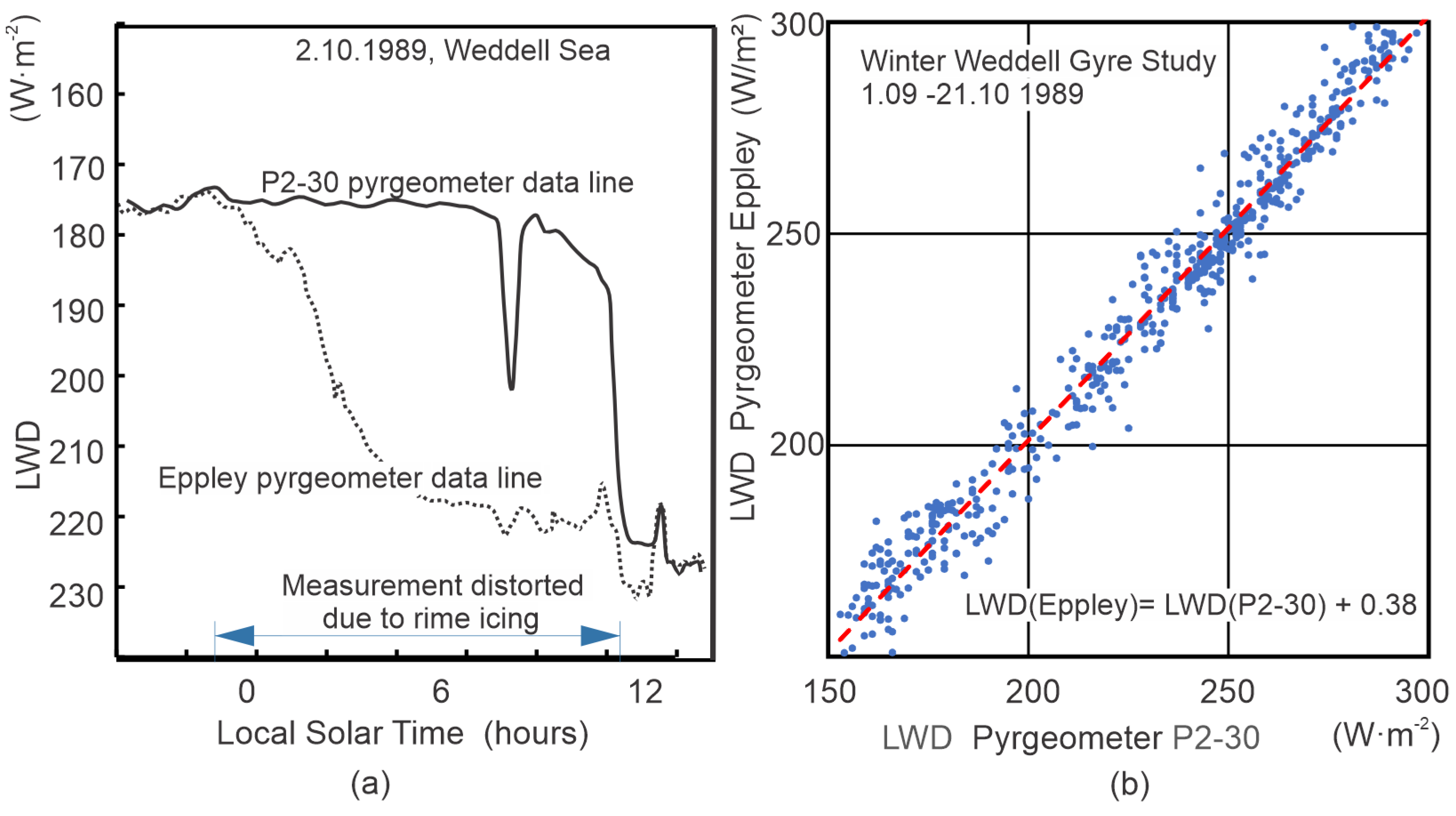
Field intercomparisons conducted [15] demonstrated that the P2-30 maintained signal stability even during intensive icing, whereas the Eppley pyrgeometer showed significant distortions under the same conditions. This is clearly illustrated in Figure 5a, where the P2-30 continued to record stable radiation during an icing episode in the Weddell Sea, while the Eppley readings noticeably degraded.
Additional confirmation of the validity of the radiation scale and its consistency with the international standard was obtained through the analysis of a long-term series of co-located measurements. A correlation analysis of nearly two months of observations (Figure 5b) revealed a steady linear correspondence between the P2-30 and Eppley data, confirming the stability and reproducibility of the P2-30 scale in real field conditions. Simultaneously, results for free hydrometeor conditions are presented. The aggregate results attest to the correctness of the P2-30 radiation scale and its alignment with the international pyrgeometer scale reproduced in Davos.
The lower boundary of the cloud cover was determined using the IMO-1 pulsed light locator, which allowed thin stratus clouds that were not visually distinguishable to be excluded from the analysis.
Temperature, humidity, and pressure profiles, obtained from aerological soundings via the D22 “Malachite” radio theodolite system [16], were used as input parameters for these calculations in an aerosol-free atmosphere.

2.3. Method of Arctic Haze Detection

In the Arctic, haze is a hard-to-observe atmospheric phenomenon: visual and standard instrumental methods do not allow it to be reliably recorded. Therefore, a key element of the study was the use of the temporal variability of longwave radiation as a diagnostic tool. This approach is based on the idea that even weak microphysical changes in the radiating layer are recorded by a pyrgeometer**, which** turns out to be sensitive to the state of the aerosol layer.
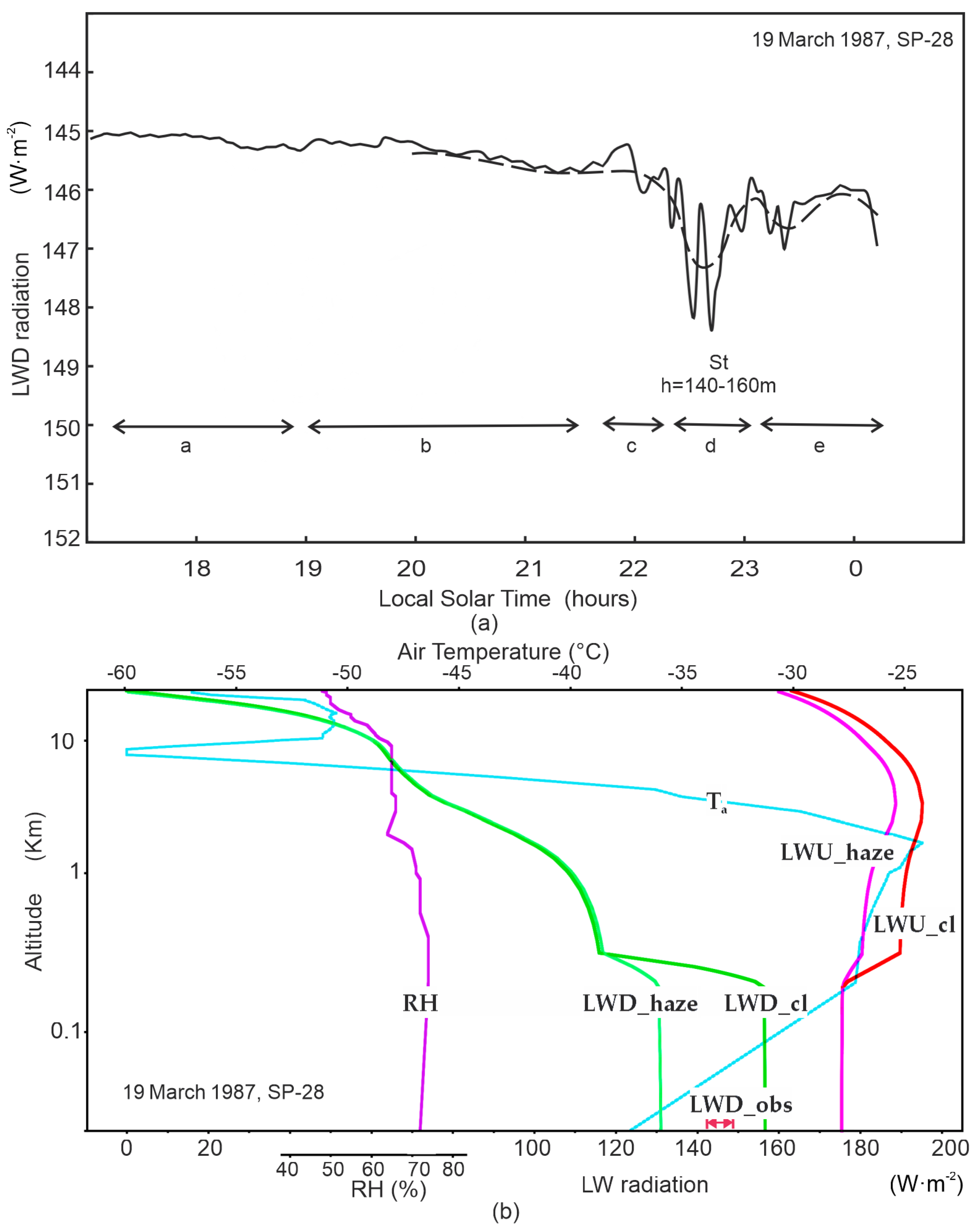
To classify the atmospheric states, the RMS was used, calculated for each hour as a deviation of the instantaneous LWD values from the mean. This parameter made it possible to quantify the level of radiation variability associated with the physical states of the surface layer (Figure 6a). Under cloudless conditions, RMS < 0.1 W·m−2—the radiation background is stable; in the presence and amplification of haze, the RMS increases to 0.2–0.7 W·m−2; when the haze passes into a thin stratus cloud, the RMS exceeds 2 W·m−2.
Thus, LWD fluctuations become an indicator not only of the presence of haze, but also, as can be assumed, the process of its microphysical evolution. It is important that during the observation period, there was no aerosol advection or changes in the concentration of condensation nuclei. Consequently, the rise in RMS reflects the internal transformations of the layer under evening cooling: particle hydration, condensation, and sublimation growth. This is the key result: the transition from haze to cloud is not accompanied by a sharp collapse of radiation but occurs in a narrow range of values. Such stability of the flux indirectly indicates the physical proximity of haze and thin stratus as two states of the same inversion layer.
This allows us to assume that Arctic haze and thin stratus are not two different modes of the phenomenon, but two adjacent states of the same evolving layer. To confirm this hypothesis, model calculations were performed, the results of which are presented in Figure 6b. In the calculations of longwave radiation, a simplified two-stream model was used, in which the optical thickness of the layer is determined by the total absorption of water vapor and CO2. The absorption coefficient of water vapor was specified as temperature-dependent, which makes it possible to correctly describe absorption variations in the lower troposphere. This approach ensures the stability of calculations in the absence of a spectral model and allows for the reproduction of a realistic vertical profile of LW fluxes. The haze parameters were set directly through modification for a layer of 150–200 m, which simulates the presence of a thin, low layer of haze. This local modification of the optical thickness makes it possible to calculate LW radiation within the calculation scheme without explicitly specifying the microphysics of the clouds. Such a layer can correspond to fog, haze, a waterlogged inversion layer, or a thin low cloud. All these types of layers have an increased concentration of water vapor or aerosols, leading to a significant increase in optical thickness in the longwave range.
In the second case, a thin cloud layer was introduced at an altitude of 150–200 m with increased emissivity, simulating the formation of a stratus cloud in the inversion zone. To describe this layer more physically, a mixed cloud phase was added to the model, including liquid water and ice crystals. In combination with increased water vapor, this forms a narrow radiatively active layer, which in the model is equivalent to a thin stratiform cloud. Calculated vertical profiles of longwave radiation based on aerological sounding make it possible to trace the formation of an additional radiating layer within the surface-based radiation inversion and to assess the differences between the haze and thin stratus modes.
Temperature and relative humidity profiles record a pronounced inversion in the lower 150–180 m and the presence of a local humidity maximum in its upper part. It is this zone that becomes the area where the emitting layer is formed in the model, determining the structure of the LWD and LWU fluxes. In haze mode, the downward flux (LWD_haze) changes slightly in the given layer. The upward flux (LWU_haze) is formed mainly by the surface, and the haze contribution is manifested only as a small additional radiation in the 140–180 m layer. When moving to a thin stratiform cloud, the character of the profiles changes. The cloud layer introduced into the model forms a pronounced maximum of downward radiation (LWD_cl) in the inversion zone, leading to a noticeable increase in LWD at the surface. This indicates that the aerosol particles were hydrated during the haze phase, and the enhanced radiative effect was due to condensation and sublimation growth. Recent studies [17] confirm this interpretation.
This also leads to an increase in the upward flux reaching the top of the atmosphere; its increase is comparable to the measured increase in longwave radiation at the Earth’s surface. Figure 6a and model calculations consistently show that Arctic haze and thin stratus have a similar effect on longwave radiation transport, as both states create an additional radiating layer within the surface-based radiation inversion. The difference between them is only in intensity: haze is a weakly radiating volume, while a thin cloud is a more powerful, but physically similar source.

2.4. Approach to Determining the Aerosol Effect

The aerosol effect on the components of the atmospheric radiative balance is evaluated by comparing measured and calculated longwave radiation characteristics. The key parameter in this comparison is the atmospheric emissivity, which represents an integrated measure of the atmosphere’s longwave emission efficiency.
The calculated emissivity (εcalc) is a dimensionless quantity obtained from the Shekhter radiative transfer model [18], which accounts only for the gaseous constituents of the atmosphere (H2O, CO2, O3, etc.) and the actual temperature profile. Aerosol contributions are not included in this calculation.
To characterize the radiative properties of the real atmosphere, the observed emissivity (εobs) was used. This dimensionless parameter describes (Equation (1)) the thermal emission efficiency of the atmospheric column and is derived from direct measurements using the Stefan–Boltzmann law:
εobs = LWD·σ−1·Ta−4,
where LWD is the downward longwave radiation measured at the surface (W·m−2), σ is the Stefan–Boltzmann constant (5.67·10−8 W·m−2·K−4), and Ta is the near-surface air temperature (K).
In contrast to the calculated (parameterized) values of εcalc, which account only for gaseous absorption, the observed emissivity εobs incorporates the combined contribution of all radiatively active components in the surface-based radiation inversion layer. These include the intrinsic emission of water vapor and trace gases, the longwave radiation of aerosol formations (Arctic haze), and the contribution of fine condensation layers and ice crystals, such as fogs and hazes.
A crucial aspect of this study is the comparison between measured and calculated atmospheric emissivity. If εobs exceeds εcalc, this indicates the presence of an additional radiating layer in the atmosphere that is not represented in the gas-only model. The difference εobs − εcalc therefore quantifies the net aerosol contribution to longwave radiation.
However, the absolute value of εobs depends on the temperature and structure of the surface-based radiation inversion, which complicates comparisons between different seasons and field campaigns. A parameter is therefore required that
  • Eliminates temperature dependence;
  • Isolates only the aerosol contribution;
  • Has a strict zero limit in aerosol-free conditions;
  • Remains dimensionless and universally applicable.
These requirements are met by the normalized longwave aerosol effect (NLAE) (Equation (2)), defined as:
NLAE = εobs − εcalc,
This normalized difference between the observed and calculated (aerosol-free) longwave flux serves as a strict indicator of aerosol influence. By definition, NLAE is a normalized parameter because it represents the difference between two dimensionless emissivity values, both of which are already scaled to the theoretical blackbody flux at the current near-surface air temperature. Obtaining reliable values requires identifying cloud-free periods. However, in polar regions, cloud detection is difficult, especially during the polar night. Moreover, standard meteorological observations do not register Arctic haze unless it reaches the surface. Under such conditions, the comparison of εobs and εcalc becomes particularly important, and NLAE is the only parameter that reliably isolates the aerosol contribution.

3. Results

The results are based on the SP-28 in situ observations and on the SHEBA and MOSAiC measurement data, which were processed and analyzed using the developed methodology.

3.1. Seasonal Evolution of Atmospheric Emissivity

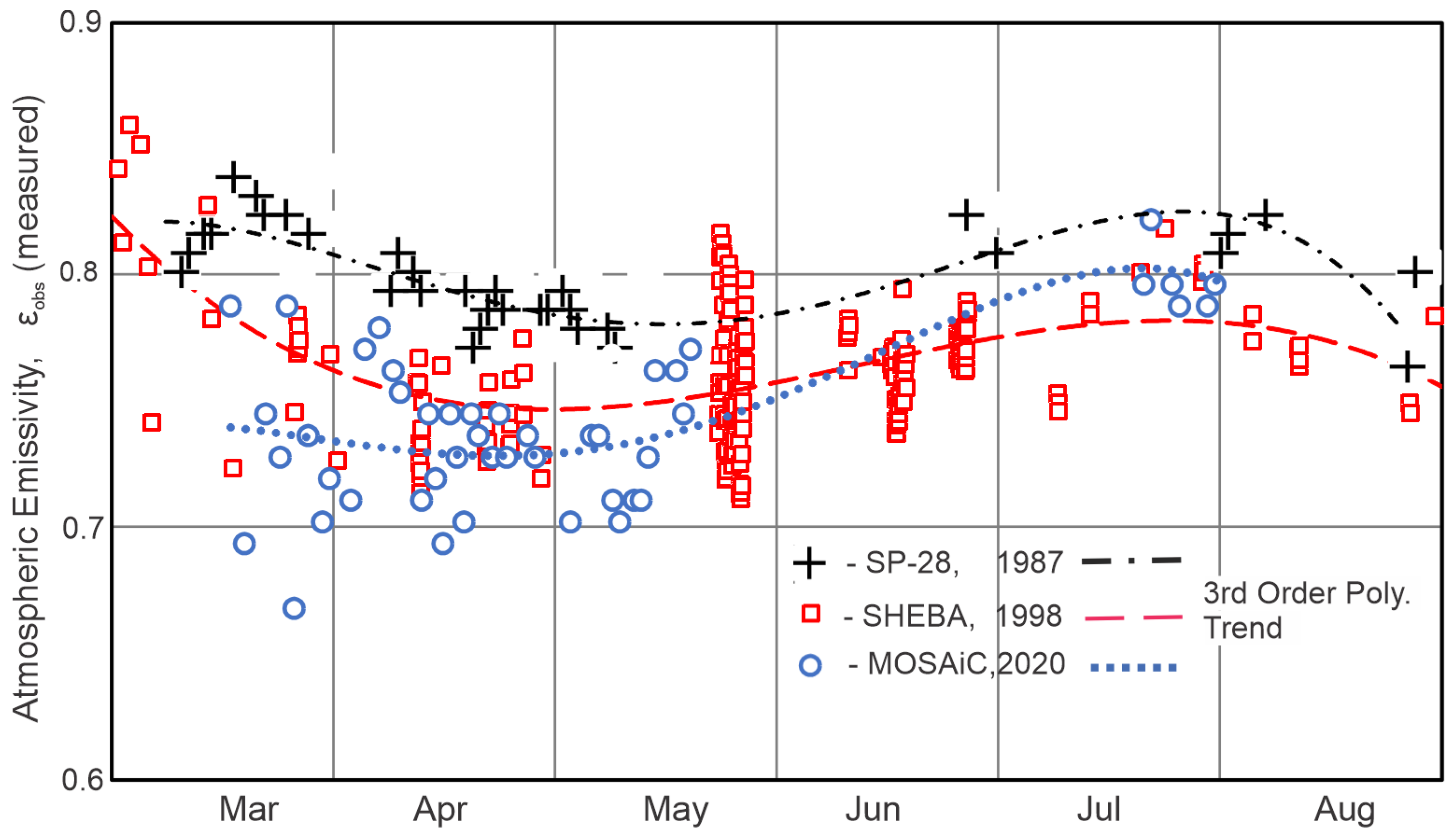
The seasonal emissivity curves obtained from the SP28 (1987), SHEBA (1997–1998), and MOSAiC (2019–2020) datasets (Figure 7) exhibit a consistent multi-decadal transformation of the radiative state of the Arctic lower atmosphere.
Each dataset is represented by a distinct marker and trend style: SP28 by black cross markers with a black dotted polynomial trend line, SHEBA by red square markers with a red dashed polynomial trend line, and MOSAiC by blue circular markers with a blue dotted polynomial trend line. These graphical distinctions allow the long-term evolution of emissivity to be traced clearly across the three expeditions.
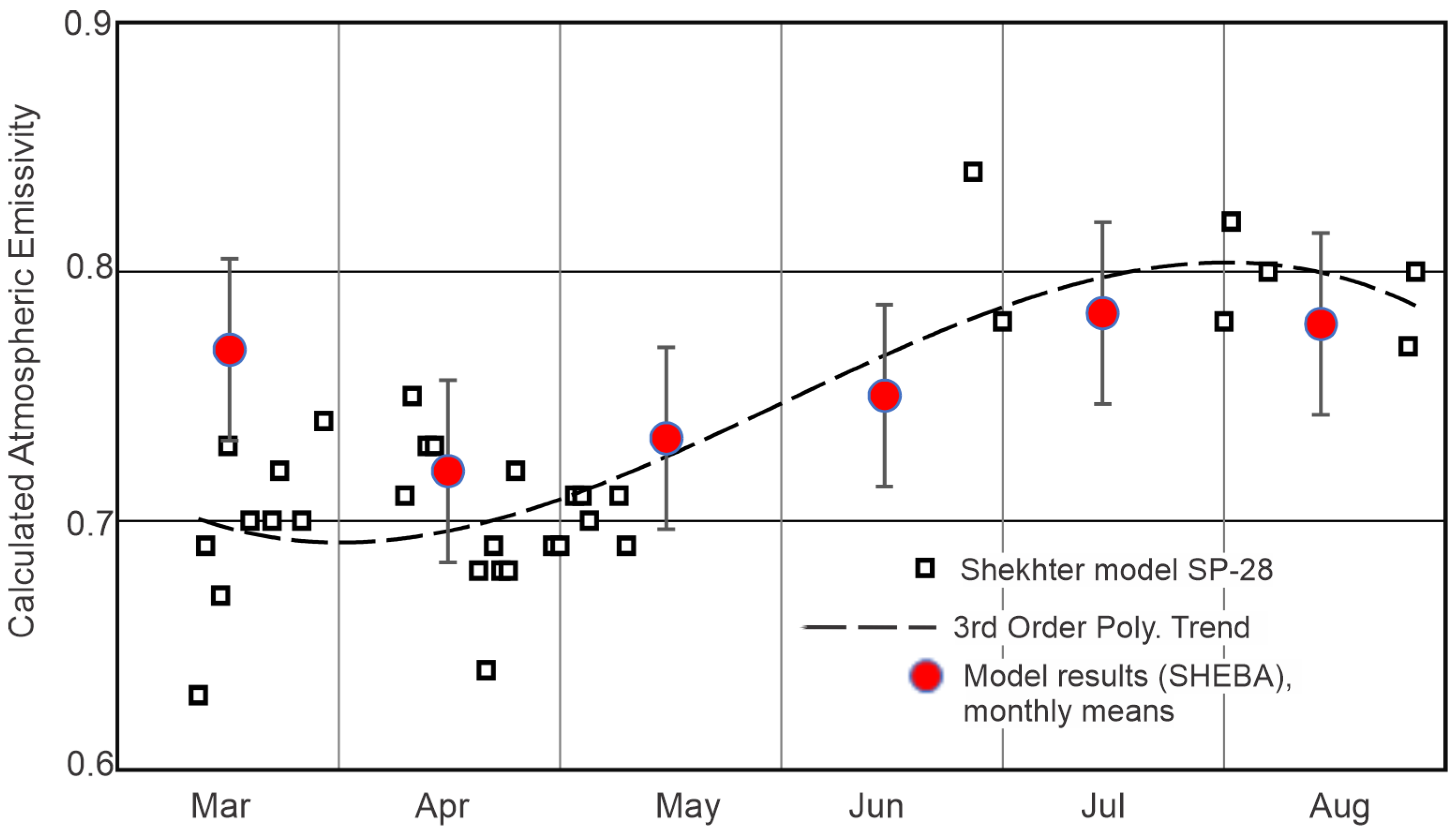
A separate comparison is provided in Figure 8, where SP-28 emissivity is plotted using black square markers representing the Shekhter model with black polynomial trend line. Additionally, we present atmospheric emissivity for the SHEBA expedition, calculated from the data in [14].
While the original study used the SBDART model (DISORT method) to obtain longwave radiation fluxes, we used those results to determine the emissivity values shown on the graph. The SHEBA expedition data are presented as monthly mean atmospheric emissivity values with confidence intervals, indicated by large red circles. Some discrepancies in the data presented in this figure are observed for March. This is because the model used by SHEBA accounts for boundary layer aerosols, whereas the Schechter model does not include an aerosol component. For other months, the values were in close agreement.
Another conclusion from Figure 8 is that emissivity trends across different epochs must be compared using only direct radiation measurements (as in Figure 7), since the schemes for accounting for aerosols and gases used in the models differ.
The SP-28 points and curve (1987) in Figure 7 therefore show the highest emissivity values during the transition season. The early spring rise is steep and forms a pronounced first peak, reflecting the accumulation of Arctic haze, the strengthening of the aerosol–condensation layer, and the strong temperature inversion typical of the 1980s. During this period, εobs lies well above the aerosol-free Shekhter model (Figure 8), indicating a substantial longwave contribution from aerosols. After this peak, the curve declines, forming a distinct April–May minimum that marks the breakdown of the haze layer and the weakening of the inversion.
The SHEBA curve (1997–1998) occupies an intermediate position. The red square markers show a reduced early spring peak compared to SP-28, and the red dashed polynomial trend line lies closer to the aerosol-free model. This indicates a transitional stage in which aerosol loading had already begun to decline, yet the haze layer still contributed measurably to longwave emission. The spring minimum becomes less pronounced.
The MOSAiC data and curve (2019–2020), represented by blue circular markers and a blue dotted polynomial trend line, show the lowest emissivity values among all expeditions. The early spring peak is nearly absent, and the entire curve closely follows the aerosol-free model. This near-perfect agreement indicates that the modern Arctic atmosphere behaves radiatively as if it were aerosol-free. The diminishment of the aerosol-driven enhancement of εobs marks the collapse of the longwave-active haze layer.
A detailed analysis of the seasonal curve shape reveals a bimodal structure with two physically distinct maxima. The first maximum, occurring from late winter to early spring, is sharp and associated with the presence of Arctic haze. Its steep rise reflects the rapid intensification of the aerosol–condensation layer and the strong temperature inversion. During this period, aerosol longwave emission becomes comparable to the gaseous contribution, producing a pronounced peak in εobs.
The second maximum, observed in June–August, is smoother and driven primarily by the seasonal increase in water vapor, the rise in the optical thickness of the gaseous atmosphere, and the diminishment of the inversion. Unlike the first peak, this maximum is almost entirely controlled by water vapor.
Thus, the bimodal structure reflects two distinct radiative regimes: an aerosol-driven early spring peak, and a water-vapor-driven summer peak.
The evolution from SP-28 to SHEBA and then to MOSAiC demonstrates a clear long-term trend: the progressive weakening and eventual diminishment of the aerosol-driven peak, consistent with the decline in transported sulfate aerosols and the degradation of Arctic haze.

3.2. Normalized Longwave Aerosol Effect (NLAE)

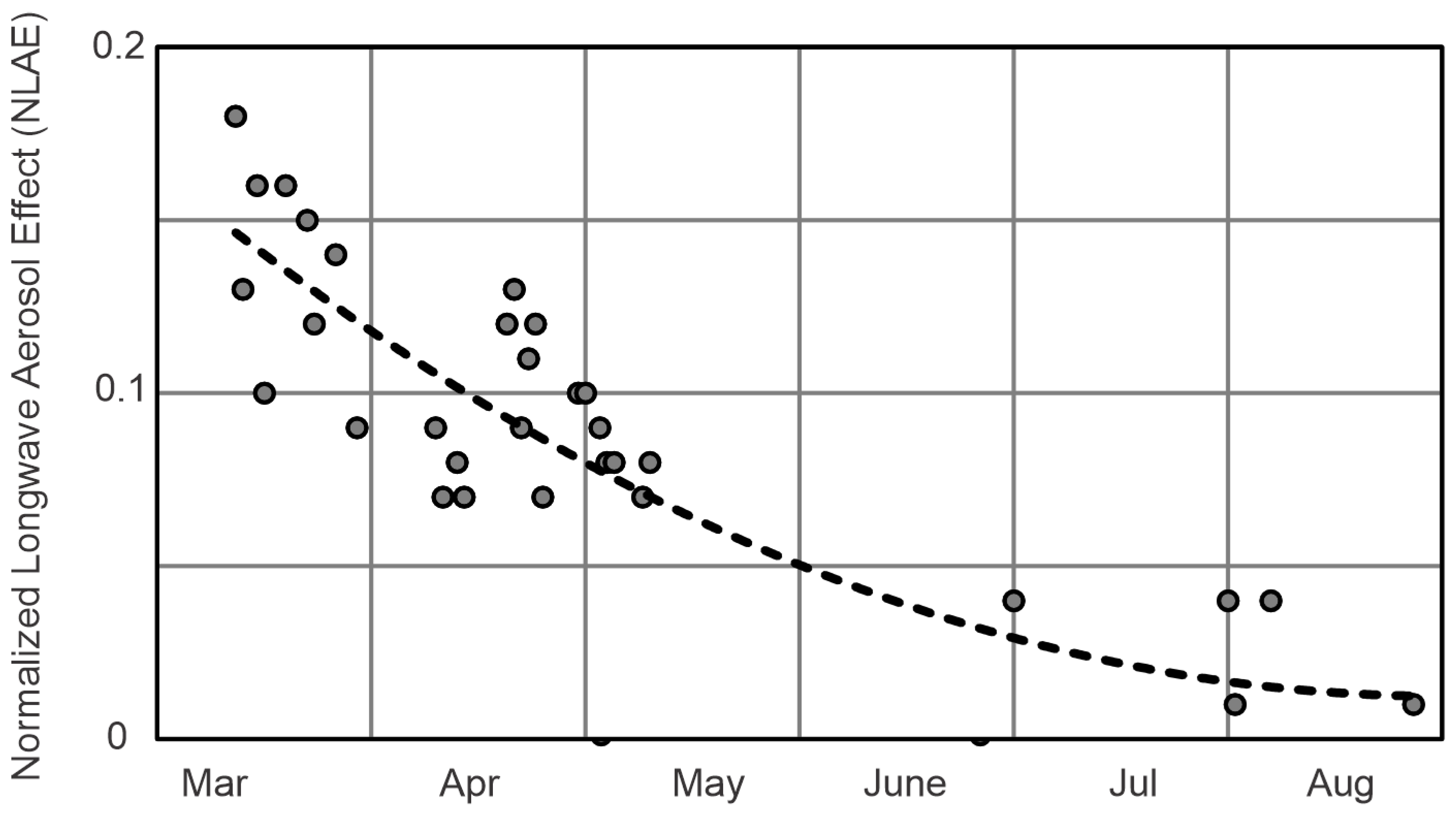
Analyzing the variability of the emissivity of the atmosphere, we paid attention to the temperature and humidity annual variability of the atmosphere. This variability, of course, is the main modulator emissivity of the atmosphere. To isolate the effect of aerosol-condensate phenomena, in particular Arctic haze, the method described in Section 2.3 was used. NLAE values calculated for SP28 show a distinct seasonal maximum in March. This corresponds to the period of maximum transport of sulfate aerosol from mid-latitudes and the most developed Arctic haze (Figure 9).
Unfortunately, we cannot provide data on the annual course of NLAE for MOSAiC and SHEBA, as calculations based on radiation models were not available to us for these datasets. Furthermore, a precise assessment requires calculations using well-validated, consistent aerosol-free models to ensure comparability of the results. However, based on the data in publication [14], which provides calculations for radiation transport models, it can be cautiously assumed that the data calculated and presented in Figure 6 are very conservative in their interannual variability.
The method is intended for retrospective analysis. It effectively identifies periods of aerosol influence and their radiative effects across different seasons.

4. Discussion

The presented results have formulated new research questions, identified relevant challenges, and outlined directions for further investigation.

4.1. Evolution of the Arctic Aerosol Regime over Time

Comparison of data from SP-28 (1987), SHEBA (1997–1998), and MOSAiC (2019–2020) shows that the radiative properties of the Arctic atmosphere have undergone fundamental changes. The most important result is that the modern εobs curve is almost identical to the calculations of the Shekhter radiative transfer model for an aerosol-free atmosphere. Such agreement is possible only in the absence of a radiatively significant aerosol layer, which in the 1980s was a defining feature of Arctic haze.
This conclusion is consistent with the long-term decline in SO2 emissions across the Arctic region, as documented by Crippa et al. [19]. Since sulfate aerosols were the dominant component of Arctic haze, the reduction in anthropogenic SO2 emissions led to the degradation of the surface-based radiation inversion aerosol layer and the weakening of its longwave radiative impact.
The magnitude and temporal structure of this decline are summarized in Table 1.

4.2. Changing the Role of Arctic Haze in Longwave Heat Transfer

During the SP-28 expedition (1987), Arctic haze produced a pronounced increase in the downward longwave flux at the surface. The LWD increment reached 15 W·m−2, substantially enhancing the integrated emissivity of the atmosphere. The highest values of the NLAE parameter were observed in March 1987, coinciding with the peak period of transboundary transport of anthropogenic pollutants from mid-latitudes.
In contrast, the modern MOSAiC data (2019–2020) indicate an almost complete absence of any aerosol contribution to longwave radiation in the central Arctic. Thus, the present-day radiative regime of the region is governed almost entirely by the gaseous composition of the atmosphere and by the temperature structure of the surface-based radiation inversion.
A physical paradox arises from this process. The downward radiation increment ΔLWD recorded at the surface is equivalent to an increase in the total heat loss of the Earth–atmosphere system to space, because any additional downward emission is accompanied by an equal additional upward emission. As a result, the integrated transmission function of the overlying layers in the infrared transparency windows is close to unity. Under these conditions, the upward longwave flux generated by the haze reaches the top of the atmosphere (TOA) almost without attenuation:
ΔLWUTOA ≈ (εobs − εcalc)·σ·Taer4,
where Taer is the kinetic temperature of the aerosol layer.
This relationship highlights that the surface-based radiation inversion aerosol simultaneously enhances the local downward radiation and intensifies the radiative energy loss of the Arctic atmosphere to space. This is also confirmed by the model calculations presented in this paper (Figure 6b).

4.3. Surface-Based Inversions Driving Longwave Atmospheric Energy Loss

The surface-based radiation inversion exerts a dual influence on the longwave radiation balance. On the one hand, it increases the downward longwave flux, thereby slowing the radiative cooling of the surface. On the other hand, having a higher temperature than the underlying surface, the inversion layer becomes the main source of upward longwave emission, enhancing the energy loss of the troposphere through the infrared transparency windows. This was clearly shown in Section 2.3.
In the 1980s, this “anti-greenhouse” effect was strongly amplified by the presence of aerosol-condensation layers, which increased the emissivity of the inversion layer. Under modern conditions, against the background of a sharp decline in aerosol concentrations, the temperature structure of the inversion is preserved, but its radiative impact is now limited exclusively to the selective emission of gases.
Thus, the “cleansing” of the Arctic atmosphere from sulfate aerosols has weakened an important channel of efficient heat release into space, which represents a significant factor in the ongoing transformation of the region’s climate.

4.4. Some Considerations Regarding the Influence of Greenhouse Gases and Aerosols on the Arctic Thermal Regime

The Arctic is warming 3 to 4 times faster than the rest of the world. The specific causes of this phenomenon remain not entirely clear. This study focuses on the relationship between anthropogenic aerosols and downward longwave radiation over the past 40 years. The influence of this radiation on surface temperature lies at the core of the “greenhouse effect” theory. Measures aimed at reducing SO2 emissions appear to have led to a decrease in aerosol concentrations. Consequently, the downward longwave flux of infrared radiation diminished, thereby resulting in a reduction of the aerosol-induced greenhouse effect. Nevertheless, the long-range transport of other pollutants—as well as their emission within the Arctic itself—continued. As these substances moved northward, natural self-cleaning processes were active; however, the rates of these processes varied for different substances.
A significant process occurring at an accelerating pace has been the occurrence of wildfires in Siberia and northern Canada. These fires are accompanied by the release of colossal volumes of combustion products (CO2, CO, CH4, and aerosols)—quantities measured in the hundreds of millions of tons or more. CO (carbon monoxide) is a product of biomass combustion, alongside CO2 (carbon dioxide) and CH4 (methane). The atmospheric residence time of CO is determined by its reaction with hydroxyl radicals and amounts to 2–3 months.
The relative changes in CO concentration—expressed as a percentage deviation from background levels—are an order of magnitude (or more) greater than those observed for the other two gases. Consequently, CO is utilized as a proxy for greenhouse gases. The absorption of CO2 by the ocean is a very slow process, spanning hundreds of years. Methane enters the atmosphere from the ocean and is removed through reactions with hydroxyl radicals; its atmospheric lifetime is 8–10 years. During the summer season, aerosols are effectively washed out of the atmosphere by precipitation within a matter of days or weeks. In the colder months, however, anthropogenic aerosols have the potential to contaminate the entire Arctic region.
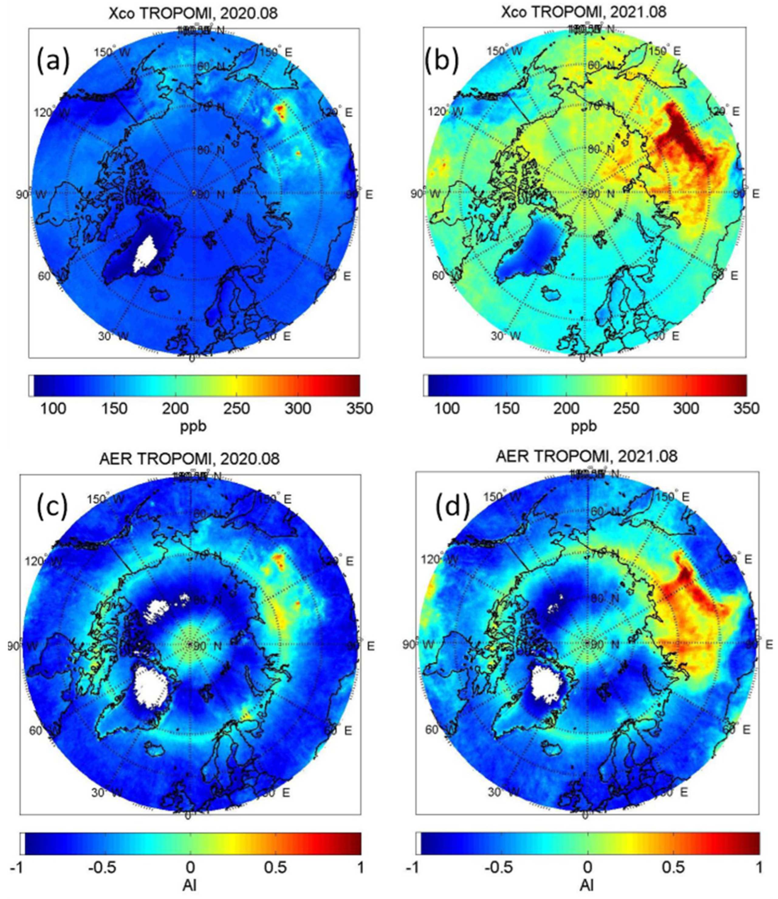
Figure 10 illustrates the significance of atmospheric self-cleaning processes in the context of the Arctic [20]. As pollutant components are transported toward the Arctic, they are simultaneously removed from the atmosphere—some more rapidly, others more slowly. In 2021, Central Siberia experienced wildfires of record-breaking intensity (Figure 10b). According to some estimates, CO emissions from Central Siberia quadrupled compared to 2020 (Figure 10a,b). These wildfires, occurring in July and August 2021, resulted in a more than twofold increase in CO concentrations—both within the Arctic and across the remainder of the Northern Hemisphere. Conversely, the impact of wildfires on Arctic aerosols during the warm season proved to be negligible; aerosol concentrations (Figure 10c,d) rose only in the immediate vicinity of the fire sources.
In summary, it can be suggested that over recent decades, the influence of greenhouse gases on the thermal balance of the Central Arctic has increased, while the influence of sulfate aerosols has declined.

5. Conclusions

The analysis of the long-term evolution of the longwave aerosol effect in the Arctic, based on a comparison of archival observations with modern measurements from the MOSAiC expedition, leads to several key conclusions.
First, the radiation regime of the Arctic has undergone a pronounced transformation over the past four decades. Whereas in the late twentieth century the Arctic haze acted as an important radiative agent, the near-zero modern values of the NLAE parameter indicate a transition toward another longwave regime.
Second, the observed decline in the aerosol effect is consistent with the global reduction in anthropogenic sulfur dioxide emissions. The decrease in sulfate aerosol concentrations in the Arctic troposphere appears to have contributed to a reduction in the integral emissivity of the atmosphere during the winter–spring period.
Third, it has been shown that surface-based radiation inversion with haze historically enhanced the longwave energy loss of the Earth–atmosphere system. By increasing the upward longwave flux through the infrared transparency windows, the aerosol layer acted as a mechanism of negative radiative feedback.
Finally, the “cleansing” of the Arctic atmosphere from sulfate aerosol—resulting from successful reductions in sulfur dioxide emissions—has led to a substantial weakening of this radiative heat-loss channel. This effect may paradoxically enhance Arctic warming, as the efficiency of longwave energy discharge into space has significantly decreased in recent decades.
These findings, supported by the spectral characteristics of outgoing radiation described in the classical works of Kondratyev (1980) [21], suggest that anthropogenic aerosol should be considered not only as a pollutant but also as an important historical regulator of the energy balance of the polar regions.

Author Contributions

Conceptualization, A.Z. and L.Y.; methodology, A.Z.; software, A.Z.; validation, A.Z.; formal analysis, A.Z.; investigation, A.Z.; resources, A.Z.; data curation, A.Z.; writing—original draft preparation, A.Z.; writing—review and editing, A.Z. and L.Y.; visualization, A.Z.; project administration, L.Y. All authors have read and agreed to the published version of the manuscript.

Funding

This research received no external funding.

Data Availability Statement

The data presented in this study are available on request from the corresponding author.

Conflicts of Interest

The authors declare no conflict of interest.

References

  1. Shaw, G.E. The Arctic haze phenomenon. Bull. Am. Meteorol. Soc. 1995, 76, 2403–2414. [Google Scholar] [CrossRef]
  2. Yurganov, L.; Rakitin, V. Two decades of satellite observations of carbon monoxide confirm the increase in Northern Hemispheric wildfires. Atmosphere 2022, 13, 1479. [Google Scholar] [CrossRef]
  3. Makshtas, A.P.; Timachev, V.F.; Zachek, A.S. Processes of air–sea interaction in polar regions. In ACSYS Conference on the Dynamics of the Arctic Climate System; WMO/TD No. 760; WMO: Geneva, Switzerland, 1994; pp. 48–53. Available online: https://epic.awi.de/id/eprint/4644/ (accessed on 15 May 2025).
  4. Andreas, E.L.; Fairall, C.W.; Guest, P.S.; Persson, O. Ice Camp Surface Mesonet NCAR PAM III 5 Minute (FINAL), Version 1.0; Arctic Data Centre: Santa Barbara, CA, USA, 2012. [CrossRef]
  5. Pirazzini, R.; Hannula, H.-R.; Shupe, M.D.; Uttal, T.; Cox, C.J.; Costa, D.; Persson, P.O.G.; Brasseur, Z. Upward and Downward Broadband Irradiance During MOSAiC; PANGAEA Dataset; PANGAEA: Bremen, Germany, 2022. [Google Scholar] [CrossRef]
  6. Wexler, H. Cooling in the lower atmosphere and the formation of polar air. Mon. Weather Rev. 1936, 64, 122–136. [Google Scholar] [CrossRef]
  7. Curry, J.A. On the formation of continental polar air. J. Atmos. Sci. 1983, 40, 2278–2292. [Google Scholar] [CrossRef]
  8. Blanchet, J.-P.; List, R. On radiative effects of anthropogenic aerosol components in Arctic haze and snow. Tellus B Chem. Phys. Meteorol. 1987, 39, 293–317. [Google Scholar] [CrossRef]
  9. Overland, J.E.; Guest, P.S. The Arctic Snow and Air Temperature Budget over Sea Ice During Winter; NOAA PMEL & Naval Postgraduate School: Seattle, WA, USA, 1991. [Google Scholar] [CrossRef]
  10. Hinzpeter, H. Report on the comparisons of radiation balance meters carried out in the Meteorological Main Observatory Potsdam. Z. Meteorol. 1953, 7, 33–48. [Google Scholar]
  11. Paltridge, G.W. A net long-wave radiometer. Q. J. R. Meteorol. Soc. 1969, 95, 635–638. [Google Scholar] [CrossRef]
  12. Zachek, A.S. On the possibility of using a pyrgeometer with a new element base in the subsystem of ground-based actinometric observations in polar regions. In Meteorological Research in Antarctica, 3rd All-Union Symposium; Part II; Gidrometeoizdat: Leningrad, Russia, 1986. (In Russian) [Google Scholar]
  13. Kipp & Zonen. CGR4 and SGR4 Pyrgeometers Instruction Manual; OTT HydroMet: Delft, The Netherlands, 2021; 44p. [Google Scholar]
  14. Intrieri, J.M.; Fairall, C.W.; Shupe, M.D.; Persson, P.O.G.; Andreas, E.L.; Guest, P.S.; Moritz, R.E. An Annual Cycle of Arctic Surface Cloud Forcing at SHEBA. J. Geophys. Res. 2002, 107, 8039. [Google Scholar] [CrossRef]
  15. Gert, K.L.; Boris Viacheslavovic, L.; Andrey, Z. Radiation measurements during the Winter Weddell Gyre Study; PANGAEA Dataset; PANGAEA: Bremen, Germany, 2010. [Google Scholar] [CrossRef]
  16. Kahl, J.D. Daily Arctic Ocean Rawinsonde Data from Soviet Drifting Ice Stations, Version 1; NASA National Snow and Ice Data Center Distributed Active Archive Center: Boulder, CO, USA, 1997. [Google Scholar] [CrossRef]
  17. Moser, M.; Voigt, C.; Eppers, O.; Lucke, J.; De La Torre Castro, E.; Mayer, J.; Dupuy, R.; Mioche, G.; Jourdan, O.; Clemen, H.-C.; et al. The Arctic Low-Level Mixed-Phase Haze Regime and its Microphysical Differences to Mixed-Phase Clouds. Atmos. Chem. Phys. 2026, 26, 1867–1887. [Google Scholar] [CrossRef]
  18. Shekhter, F.N. On the calculation of radiant heat fluxes in the atmosphere. Tr. Gl. Geofiz. Obs. 1950, 22, 38–52. (In Russian). Available online: https://mgmtmo.ru/edumat/MGO/Works_MGO_22.pdf (accessed on 28 September 2025).
  19. Crippa, M.; Guizzardi, D.; Pagani, F.; Banja, M.; Muntean, M.; Schaaf, E.; Becker, W.E.; Monforti-Ferrario, F.; Quadrelli, R.; Risquez Martin, A.; et al. EDGAR v8.0 Global Air Pollutant Emissions; European Commission, JRC: Brussels, Belgium, 2023. [Google Scholar] [CrossRef]
  20. European Space Agency (ESA). Sentinel5P TROPOMI Level2 Products, 2020–2021. Available online: https://sentinels.copernicus.eu/ (accessed on 21 February 2026).
  21. Kondratyev, K.Y. Radiative Factors of Modern Global Climate Changes; Gidrometeoizdat: Leningrad, Russia, 1980. (In Russian) [Google Scholar]
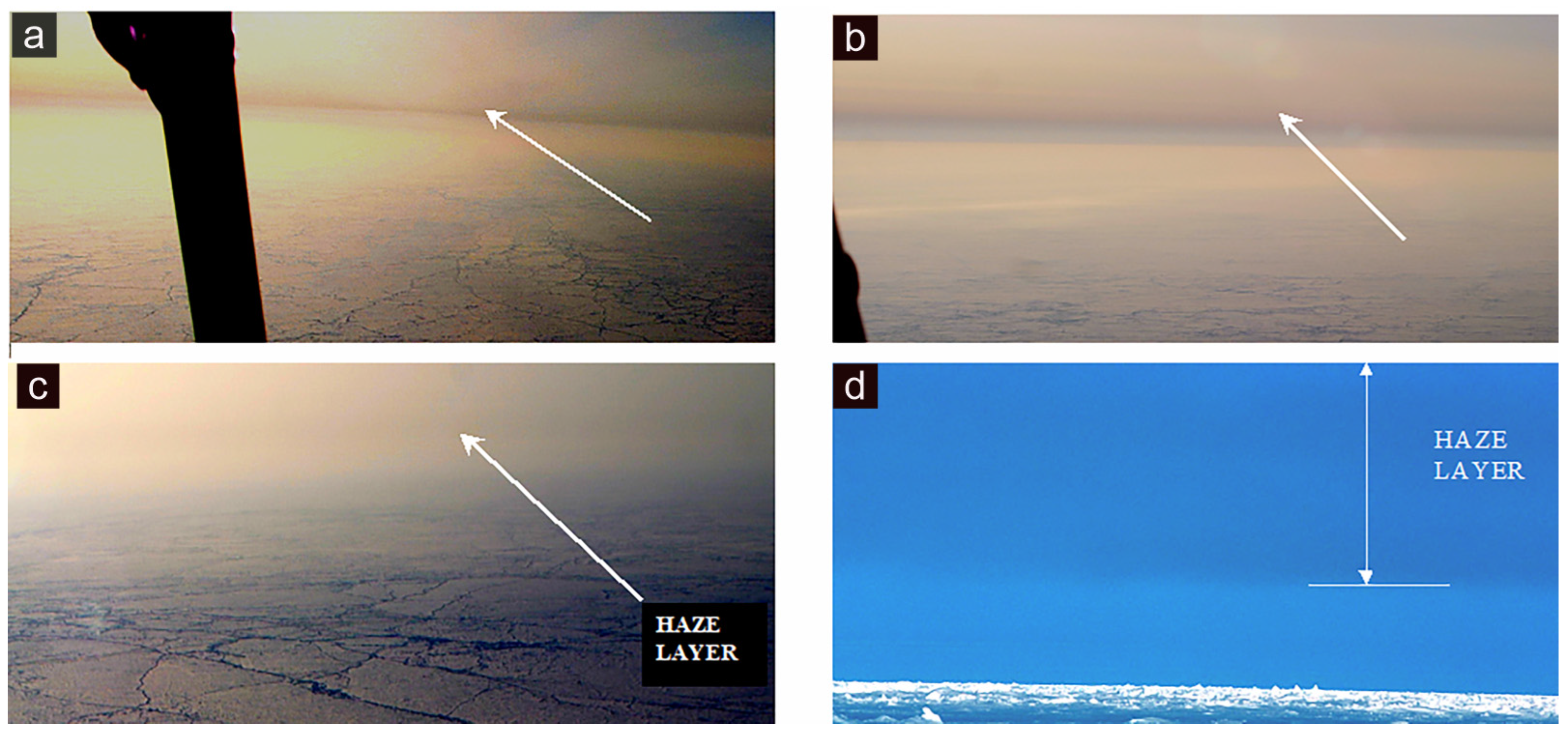
Figure 1. Visual observations of Arctic haze layers at distinct altitudes and the Earth’s surface, photographed by the author from an ultralight trike near the North Pole, 17–19 April 2001, during in situ sampling: (a)—altitude 350 m; (b)—altitude 400 m; (c)—altitude 180 m; (d)—the Earth’s surface.
Atmosphere 17 00513 g001
Figure 2. (a) Drift area of the North Pole-28 scientific station and (b) radiation measurement site, 1987.
Atmosphere 17 00513 g002
Figure 3. Mean synoptic situation and aerosol transport in March: (a) air mass trajectories from the Norilsk industrial zone to the SP-28 station, manually calculated using the back-trajectory method; (b) mean surface pressure field.
Atmosphere 17 00513 g003
Figure 4. Pyrgeometer P2-30 (1.8–30 μm).
Atmosphere 17 00513 g004
Figure 5. Field comparison results between the P2-30 and Eppley pyrgeometers: (a) Time series of longwave downward radiation (LWD) flux (W·m−2) recorded on 2 October 1989 in the Weddell Sea. The dashed line indicates the Eppley pyrgeometer signal degradation during a rime icing event, while the solid line shows the P2-30 stability. Note: the vertical axis is inverted. (b) Scatter plot and linear regression analysis of LWD data (W·m−2) obtained during the Winter Weddell Gyre Study (1 September 1989–21 October 1989). The regression equation LWD(Eppley) = LWD(P2-30) + 0.38 demonstrates high correlation and minimal systematic bias between the two instruments.
Atmosphere 17 00513 g005
Figure 6. Evolution of Arctic haze into stratus clouds: observations and modelling. (a) Time course of downward longwave radiation (LWD) on 19 March 1987. Regions a–e reflect the stages of haze evolution: (a) cloudless conditions, (b) monotonic decline of LWD (c) transition from haze to cloud forms, (d) occurrence of backscatter at 140–160 m according to ceilometer data, (e) visual recording of stratus. (b) Radiosonde observed profiles: air temperature (Ta) and relative humidity (RH). Calculated profiles of downward (LWD_haze, LWD_cl) and upward (LWU_haze, LWU_cl) longwave radiation for the Arctic haze mode and a thin stratus cloud with a lower boundary of 140–180 m and a thickness of 50 m.
Atmosphere 17 00513 g006
Figure 7. Seasonal variations in cloud-free atmospheric emissivity (measurements).
Atmosphere 17 00513 g007
Figure 8. Atmospheric emissivity: Shekhter aerosol-free model (SP-28) compared with SBDART model incorporating aerosol effects (SHEBA).
Atmosphere 17 00513 g008
Figure 9. Seasonal course of the normalized longwave aerosol effect (NLAE) for SP-28.
Atmosphere 17 00513 g009
Figure 10. Data from TROPOMI/Sentinel-5 Precursor for August 2020 and 2021; (a,b) monthly maps of CO concentrations averaged over the atmospheric total column; (c,d) corresponding maps for the Aerosol Index.
Atmosphere 17 00513 g010
Table 1. Estimated Anthropogenic SO2 Emissions in the Arctic Region (above 60° N), 1980–2020.
YearSO2(Mt/yr)Main Contributing Factors
19803.15Peak of industrial activity; minimal emission controls.
19852.90Initial implementation of regional air quality protocols.
19902.55Industrial restructuring in the post-Soviet Arctic.
19952.20Economic recession in major northern mining hubs.
20002.12Stabilization of smelting operations in Norilsk.
20052.05Start of local technological upgrades in metallurgy.
20101.88Modernization of non-ferrous metal production.
20151.75Phasing out of obsolete smelting capacities.
20201.52Implementation of IMO 2020 (maritime fuel sulfur cap).
Disclaimer/Publisher’s Note: The statements, opinions and data contained in all publications are solely those of the individual author(s) and contributor(s) and not of MDPI and/or the editor(s). MDPI and/or the editor(s) disclaim responsibility for any injury to people or property resulting from any ideas, methods, instructions or products referred to in the content.