Mobile Observations of Air Pollution in an Urban Area: Characteristics and Variability

Abstract

Urban air pollution exhibits pronounced spatial heterogeneity, yet conventional fixed-site monitoring often cannot resolve fine-scale hotspot patterns. To address this issue, this study conducted a winter intensive observation campaign combining mobile measurements and synchronous fixed-site observations in Chengdu. The mobile observation was used to characterize the spatial distribution of particulate pollution, while fixed-site pollutant and meteorological data were used to provide temporal and background context. Three mobile observation sessions were performed each day at fixed local times (09:00–11:00, 14:00–16:00, and 19:00–21:00). Based on the PM_2.5 concentration, the observation period was categorized into two episodes: polluted episodes (PM_2.5 > 75 μg m⁻³) and clean episodes (<75 μg m⁻³). Polluted episodes were characterized by substantially elevated PM_2.5, PM₁₀, NOx, CO, and particle number concentrations, together with relatively weak wind speed, indicating enhanced accumulation under stagnant conditions. In contrast, clean episodes generally occurred under stronger ventilation and lower pollutant levels. The results revealed marked small-scale spatial variability and distinct temporal changes in particulate pollution. PCA was suitable for the dataset (Kaiser–Meyer–Olkin = 0.788; Bartlett’s test, p < 0.001), and the first three principal components explained 82.7% of the total variance. Cluster analysis further identified three pollution regimes among 224 samples: clean/ventilated (34.4%), intermediate accumulation (39.7%), and heavy accumulation (25.9%). These findings demonstrate that short-term intensive mobile monitoring can serve as a cost-effective supplement to conventional monitoring for hotspot identification and targeted urban air-pollution management.

1. Introduction

Both particulate matter (PM) and ozone (O₃) are major components of atmospheric pollution and are closely related to human life and the environment. Long-term exposure to PM and O₃ can lead to bronchitis [1], affect the nervous system [2], and even cause cancer [3]. High levels of PM_2.5 can cause serious visibility problems in large cities, resulting in an increase in traffic accidents [4]. Air pollution can be affected by various factors, such as meteorological conditions, anthropogenic factors, and geographic locations [5,6,7]. Human activities are a primary source of emissions [8], and meteorological conditions are also an external cause of air pollution. A negative correlation between meteorological conditions, including temperature, air pressure, wind speed (WS), and PM_2.5 concentrations has been reported in the Sichuan Basin, with the exception of relative humidity (RH), which shows a positive correlation with PM_2.5 [9,10]. To better understand the sources contributing to PNC events, source apportionment is essential, especially in the Sichuan Basin [11,12]. High O₃ pollution is caused by the contributions of gaseous precursors, high temperatures, low RHs, and low wind speeds [13]. Despite improvements in air quality driven by enhanced pollution control measures, urban pollution continues to occur frequently, especially in winter. Sources of PM and O₃ can be identified via particle number concentration (PNC) and other pollutant analyses. Particle source apportionment based on PNC has become increasingly mature and is complementary to and verifiable against mass concentration-based apportionment [14]. Instruments such as scanning mobility particle sizers (SMPS), condensation particle counters (CPC), differential mobility analyzers (DMA), and ion chromatography (IC) have been used in studies on particle number concentration (PNC), which is essential [15]. Current techniques for source apportionment include receptor model factor analysis (FA) [16,17], positive matrix factorization (PMF) [18,19,20], and principal component analysis (PCA) [21]. In recent aerosol studies, PCA has been widely used as an effective exploration tool to reduce data dimensionality, reveal covariance structures among measured variables, and identify potential source-related patterns in PM_2.5 and aerosol-bound metals [22,23]. Therefore, PCA provides a useful framework for distinguishing dominant aerosol regimes and inferring the major processes controlling aerosol characteristics.

Street-level air pollution has attracted significant attention in recent years [24]. Effectively simulating air pollution distribution has been one of the key challenges for researchers. Some methods (e.g., WRF models) have been used to calculate air pollution distributions, and some models have been used to track sources [25,26,27]. However, these methods are not applicable to some micro areas that lack monitoring data [28]. To precisely identify pollutant sources, mobile observations—employing detection instruments mounted on vehicles to collect data—provide a highly effective method for analyzing the origins and dispersion patterns of atmospheric pollutants with finer granularity. This approach provides insights into spatial variabilities that are inaccessible through fixed-site monitoring [29,30,31]. It also allows for the expansion of monitoring coverage to specific areas of interest [32,33,34]. Julie et al. reported that roadways are the primary source of NOx emissions, with vehicles on roads being the major contributing source, whereas industries predominantly contribute to SO₂ emissions [35]. Luz et al. reported that the PNC, NOx, black carbon (BC), and CO levels are highest during winter; lowest during summer and autumn; higher on weekdays than on weekends; and higher during morning rush hours than at other times [36]. However, the PM_2.5 concentrations do not exhibit the same pattern [36]. Multiple observations conducted on the Yangtze River have indicated that the primary variations in PM_2.5 levels are largely due to geographical differences and distinct anthropogenic emission sources [37]. The number of mobile observations was slightly lower than that obtained through fixed-site measurements [38]. Extensive research has been conducted on O₃ pollution monitoring, but there remains a gap in the use of mobile observation methods to capture the sources of pollutants precisely.

Chengdu is located in the Sichuan Basin and is surrounded by mountains, which restricts air dispersion and leads to the accumulation of pollutants. The city also experiences minimal winds throughout the year, further exacerbating this issue [39]. The primary sources of air pollution in Chengdu are industry and traffic. The geographical environment, rapid economic development and high number of vehicles (over 5 million) significantly contribute to air pollution [40]. Therefore, local traffic emissions are a major source of NO₂ pollution [41], and the relationship between air pollution and NO₂ levels is complex. Pollution levels are typically measured with fixed stations, which are usually few in number and offer limited coverage [35]. Owing to the presence of buildings, traffic, and commercial areas, the pollution concentrations recorded by fixed stations may not reflect the overall pollution levels across the entire area. Megacities such as Chengdu face the challenge of dynamic air pollution, which varies across time and space. Fixed stations, although useful, cannot adequately capture this variability because of their limited coverage and lack of flexibility. This approach is particularly relevant for a city such as Chengdu to combine mobile observations with fixed station observations.

In this paper, we conducted a study that utilized a severe pollution event in the Shuangliu District in Chengdu. In winter 2022, district-wide mobile observations were initiated to measure PNC and O₃ concentrations. Section 2 introduces the monitoring locations, observation instruments, and methods used. Section 3 investigated the spatial distributions of the atmospheric pollutants in the Shuangliu District and identified the potential source contributions, and backward trajectory analysis was performed. Section 4 summarizes the findings of this study.

2. Materials and Methods

2.1. Experimental Location

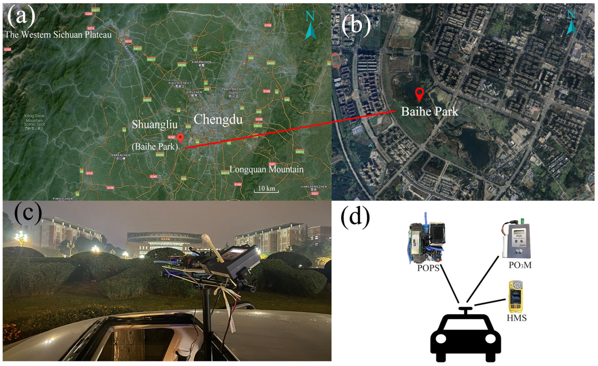
Chengdu is situated in the Sichuan Basin and hosts a population of approximately 21,403 million people. Chengdu provides a typical mixing area for effective air pollution, as it has many vehicles, numerous industries and conditions for air pollution accumulation. Figure 1a shows the location of Chengdu and the observation area in Shuangliu District. Chengdu is situated in the western Sichuan Basin, bordered by the Western Sichuan Plateau and Longquan Mountain, where the basin-like terrain can limit pollutant dispersion under stable atmospheric conditions. Figure 1b shows the fixed observation site in Baihe Park (30.35° N, 103.54° E, 495.8 m a.s.l.) and its surrounding environment. The site is located in an urban–suburban transition area with nearby residential areas, roads, green space, water bodies, and Shuangliu International Airport, reflecting a mixed-source environment suitable for mobile and fixed observations of particle number concentration and O₃. The station recorded six pollutant parameters (PM_2.5, PM₁₀, SO₂, NO, CO, and O₃) with hourly time resolution. In addition to these gaseous and particulate pollutants, the station also measured basic meteorological data such as temperature, relative humidity (RH), wind speed, and atmospheric pressure, which were also recorded on an hourly basis. For the mobile observations, PNC (particle number concentration) and O₃ concentrations were recorded in real time, with data captured at a second-level resolution. These measurements, taken from both the fixed and mobile stations, were crucial for analyzing the spatial and temporal variations in air pollution and understanding the influence of meteorological conditions. The site location is shown in Figure 1.

2.2. Mobile Observation Instruments

During the mobile observations, the portable optical particle profiler (POPS), personal ozone monitor (PO₃M), and hand-held meteorological station are outfitted outside the vehicle via a bracket, which extends approximately 0.5 m out of the car top cover. This configuration permits measurements of aerosol particle concentrations, O₃ concentrations, light intensities, and fundamental meteorological variables outside the vehicle overflow. The instruments and their placement are shown in Figure 1d. Fixing equipment outside the car top effectively prevents contamination from vehicle exhaust itself. On the basis of the air pollution data and warning levels released by the Chengdu Environmental Protection Bureau, close attention was given to the heavy pollution period. Intensified mobile observations were conducted during heavy pollution events and focused on the key areas where air pollution problems occur. Repeated validations were performed in areas with anomalous data observations to ensure data reliability. To mitigate any potential issues related to airflow turbulence, we equipped the POPS with an additional airflow pump. This pump helps to stabilize the flow of air into the instrument, preventing any disturbance that could affect the measurements. Additionally, the inlet tube was positioned towards the rear of the vehicle, further reducing the impact of vehicle motion and external airflow on the data.

The POPS is an optical instrument produced by Nanjing Handix Environmental Technology Co., Ltd. (Nanjing, China). and is used for measuring aerosol particle size spectra. POPS provides particle size data in the range of 130 nm⁻³ μm, which are divided into 16 channels. POPS, as an observational instrument, maintains reasonable accuracy during motion [31,42]. In addition, we calibrated the instrument using standard particles prior to the mobile observations.

The O₃ analyzer used in this mobile observation experiment was a pocket-sized PO₃M (2B Tech. Ltd., Broomfield, CO, USA). The hand-held meteorological station used WHS1000, a wearable multifunctional pocket-sized meteorological instrument developed by Zoglab Technology Co., Ltd. (Hangzhou, China). The PO₃M mainly measures the O₃ concentrations during mobile observations, whereas the hand-held meteorological station provides temperature, RH, UV intensity, and radiation intensity data. Equipment specifications are presented in

Table 1. Mobile observation instruments’ parameters.

Hand-Held Weather Station		PO3M		POPS
Temperature measurement range	−30–70 °C	Measurement	UV absorption at 254 nm	Range	0.13–3 μm
RH measurement range	0–100% RH	Linear dynamic range	0 ppb~10 ppm	Channel	15
Press measurement range	300–1100 hPa	Resolution	0.1 ppb	Laser wavelength	402 nm
Lighting dynamic range	0–128,000 lx	Accuracy	Greater of 1.5 ppb	Time Interval	1 s
UV Wavelength range	0.28–40 nm	Measurement intervals	10 s	Diameter resolution	5%
UV Exponential level	0–20	Measure frequency	0.1 Hz	Flow Rate	0.05–0.35 LPM

.

2.3. Experimental Methods

During the observation period, our primary focus was on the hourly fluctuations in pollutant levels at Baihe Station in Shuangliu from 21–30 December (shown in Table S1). Three mobile observation sessions were conducted daily: morning (9:00–11:00), afternoon (14:00–16:00), and evening (19:00–21:00). Each session commenced at Chengdu University of Information Technology and traveled to various schools, tunnels, airports, and expressways. Approximately 40 min after departure, the route reached Baihe Park, where we circled to collect data. Additionally, instruments were stationed in Baihe Park to measure meteorological elements and pollutant data, serving as supplementary validations for mobile observations and for the source apportionment of pollutants.

The mobile observation was designed as a short-term intensive winter observation period. Winter is generally the most polluted season in Chengdu, with meteorological conditions that are more favorable for pollutant accumulation (as shown in Figure S1). Therefore, this observation period was selected to capture fine-scale spatial heterogeneity of air pollution under pollution-prone seasonal conditions. The selection of the campaign period also considered fieldwork scheduling, instrument deployment conditions, and the substantial variability of winter pollution levels. It should be noted that the mobile observations were not intended to represent annual conditions. Precipitation can strongly affect particulate concentrations. During the field campaign, mobile observations were suspended during rainfall periods to avoid direct interference from wet conditions. Because quantitative precipitation measurements were not available, rainfall was not included as an explicit variable in the present analysis.

2.4. Data Validation and Quality Control

A variety of processing operations are needed, including tasks such as GPS instrument interpolation and calibration. For the mobile observations, we used a smartphone app to record the trajectories, which was mounted on the roof of the vehicle. During mobile observations, notably when traversing tunnels, intermittent loss of GPS signals may occur. To counteract this, a linear interpolation methodology is applied to seamlessly bridge the gaps in the data. The PO₃M is equipped with an integrated GPS system, which allows direct data reflection on roadways. Nonetheless, discrepancies emerge between the depicted spatiotemporal distribution map of the O₃ concentrations and the actual distributions. The observers rectify this by adjusting the initial point coordinates, thereby refining the latitudes and longitudes for the entire route and facilitating data calibration. The assessment of GPS precision and synchronization of measurement devices pose formidable challenges. Especially in urban environments, geographic features and structures can impede signals, which makes accurate quantification of signals challenging. With vehicle mean speeds maintained at 40 km h⁻¹, the impact on the GPS accuracy and interpolation efficacy is minimal [30]. It should be noted that mobile observation measurements may be affected by vehicle speed and vehicle-induced turbulence near the sampling inlet, which introduces additional uncertainty compared with fixed-site observations.

2.5. Comprehensive Analysis of Meteorological Data

The Shuangliu Meteorological Bureau provides minute-level quality control data for the Shuangliu National Station, which includes the basic elements (temperature, RH, and pressure) and pollution parameters (CO, SO₂, and NOx). ERA5 is a fifth-generation atmospheric reanalysis dataset that is produced by the European Centre for Medium-Range Weather Forecasts (ECMWF). The reanalysis data were downloaded from the official website of ECMWF (https://cds.climate.copernicus.eu, accessed on 14 October 2023) to obtain the PBLH information. To analyze and assess the sources of atmospheric pollutants, this study incorporated additional meteorological data more accurately. Cloud and other meteorological data obtained from the Russian meteorological website (http://rp5.ru, accessed on 8 January 2023) can fill observational gaps related to cloud cover, visibility, and weather conditions on a daily basis. Both cloud data and wind information also provide valuable references for categorizing pollution weather conditions.

The global reanalysis meteorological data that were downloaded from the official websites of the National Oceanic and Atmospheric Administration (NOAA) and Air Resources Laboratory (ARL) (https://www.ready.noaa.gov/HYSPLIT.php, accessed on 9 August 2024) were used for backward trajectory model (HYSPLIT) analyses. Starting from Baihe Park, 24 h and 48 h backward trajectories were calculated to determine the sources and paths of the pollutants.

2.6. Principal Component Analysis

Principal component analysis (PCA) of a data matrix extracts the dominant patterns in the matrix in terms of a complementary set of score and loading plots [43]. PCA was conducted using the matched hourly dataset to investigate the covariance relationships among PNC, gaseous pollutants, particulate matter, and meteorological variables in this study. All variables were first standardized using z-score transformation to remove the influence of different units and scales. Principal components with eigenvalues greater than 1 were retained. The variance explained by each component and the corresponding loading matrix were used to identify the dominant variables and interpret the major patterns in the dataset.

PCA was performed on the standardized dataset. Before PCA, all variables were standardized using z-score transformation to remove the influence of different units and scales, so that each variable had a mean of 0 and a standard deviation of 1 [44]. Each variable was first normalized using z-score transformation:

$$Z_{ij}={\displaystyle \frac{X_{ij}-{\overline{X}}_j}{s_j}}$$

$X_{ij}$ represents the original value of the j-th variable for the i-th sample. ${\overline{X}}_j$ is the mean value of the j-th variable across all samples, and $s_j$ is the corresponding standard deviation.

Each PC can be expressed as follows:

$$P{C}_k=a_{1k}{Z}_1+a_{2k}{Z}_2+L+a_{pk}{Z}_p$$

where PC_k is the k-th PC; Z_p is the p-th predictor variable, and a_pk is the coefficient of Z_p [45].

Considering that the present dataset was derived from a short-term intensive mobile observation, PCA was ultimately selected as the main method because it is more suitable for identifying dominant co-variation patterns in a relatively limited dataset. Because the dataset was obtained during a short-term intensive winter campaign, the results should be interpreted within the scope of the observation period. The measurements are well suited to identifying fine-scale spatial heterogeneity and localized pollution hotspots, but they do not provide a temporally comprehensive characterization of urban air quality. In particular, the observed hotspot behavior, pollutant co-variation, and meteorological associations may be influenced by campaign-specific conditions and therefore cannot be directly generalized to other seasons or longer periods without additional observations.

2.7. Trajectory

2.7.1. Concentration Weight Trajectory

The concentration weight trajectory (CWT) calculates the average concentration of each pollutant within the trajectory associated with the grid, and the residence-time weighted concentration is allocated to each grid cell.

$$\mathrm{In}\left({\stackrel{-}{\mathrm{C}}}_{\mathrm{ij}}\right)={\displaystyle \frac{1}{{{\displaystyle \sum }}_{\mathrm{k}=1}^{\mathrm{N}}{\mathsf{\tau }}_{\mathrm{ijk}}}}{\displaystyle {\displaystyle \sum }_{\mathrm{k}=1}^{\mathrm{N}}}\mathrm{In}\left({\mathrm{C}}_{\mathrm{k}}\right){\mathsf{\tau }}_{\mathrm{ijk}}$$

where $\mathrm{i}$ and $\mathrm{j}$ are the indices of the grid, $\mathrm{k}$ is the index of the trajectory, $\mathrm{N}$ is the total number of trajectories used in the analysis, ${\mathrm{C}}_{\mathrm{k}}$ is the pollutant concentration measured upon arrival at trajectory $\mathrm{k}$, and ${\mathsf{\tau }}_{\mathrm{i}\mathrm{j}\mathrm{k}}$ is the residence time of trajectory $\mathrm{k}$ in the grid cell (i, j). High ${\overline{\mathrm{C}}}_{\mathrm{i}\mathrm{j}}$ values mean that air parcels passing over cell (i, j) would, on average, cause high concentrations at the receptor site [46].

2.7.2. Potential Source Contribution Function

The potential source contribution function (PSCF) is an effective method for calculating the contributions of potential sources [47,48]. The PM_2.5 and the aerosol particles are located at grid cell (i, j), and an air parcel passing through that location indicates that material from the source can be collected and transported along the trajectory to the receptor site. The PSCF value for c (i, j) was defined as

$$PSC{F}_{ij}={\displaystyle \frac{M_{ij}}{N_{ij}}}{W}_{ij}$$

where ${\mathrm{M}}_{\mathrm{i}\mathrm{j}}$ is the number of endpoints for c (i, j) with arrival times at the observation site, corresponding to pollutant concentrations higher than an arbitrary criterion value. ${\mathrm{N}}_{\mathrm{i}\mathrm{j}}$ is the total number of trajectory segment endpoints that fall within c (i, j). To reduce the random error and uncertainty of the small value of ${\mathrm{N}}_{\mathrm{i}\mathrm{j}}$, the weighting function of ${\mathrm{W}}_{\mathrm{i}\mathrm{j}}$ reduces the PSCF values when the total number of endpoints in a particular cell ${\mathrm{N}}_{\mathrm{i}\mathrm{j}}$ is approximately 3 times less than the ${\mathrm{N}}_{\mathrm{i}\mathrm{j}}$ average value ${\mathrm{N}}_{\mathrm{A}\mathrm{v}\mathrm{e}}$ of the endpoints per cell [49].

$$W_{ij}=\left\{\begin{array}{c}1.0,\\ 0.70,\\ 0.42,\\ 0.17,\end{array}\begin{array}{l}{N}_{ij}>3N_{Ave}\hfill \\ 1.5N_{Ave}<N_{ij}<3N_{Ave}\hfill \\ N_{Ave}<N_{ij}<1.5N_{Ave}\hfill \\ 0<N_{ij}<N_{Ave}\hfill \end{array}\right.$$

It should be noted that the PSCF and CWT analyses in this study were conducted using receptor-site hourly PM_2.5 and O₃ concentrations, and therefore represent pollutant-based potential source regions rather than factor-specific trajectory maps.

3. Results and Discussion

3.1. Time Series of Pollutant and Meteorological Parameters

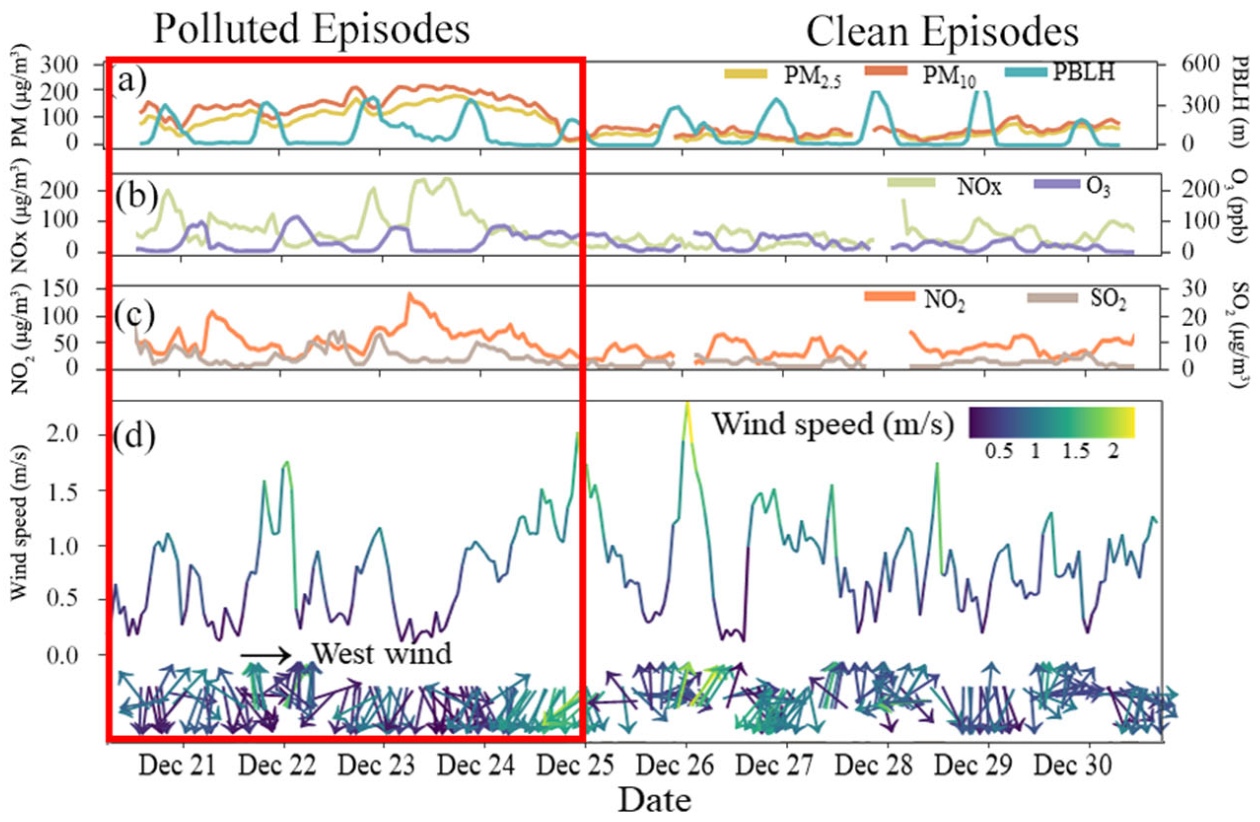
The time series of the PM_2.5, PM₁₀, and pollution parameters collected by the fixed station from 21–30 December 2022 are depicted in Figure 2. On the basis that the PM_2.5 level exceeded 75 μg m⁻³, we divided the observation period into polluted episodes (from December 21 to 24) and clean episodes (from 25–30 December). In winter, the lower altitude of the planetary boundary layer leads to a reduction in or inhibition of pollutant dispersion and serious PM_2.5 in the Sichuan Basin [40]. During the polluted episodes, the PM_2.5 concentrations reached their maximum at 196 μg m⁻³, whereas the PM₁₀ concentrations peaked at 230 μg m⁻³. When a rainfall event occurred, the PM_2.5 concentration decreased to 27 μg m⁻³. During the clean episodes, the PBL led to the accumulation of PM_2.5 concentrations again, increasing from 21 μg m⁻³ to 76 μg m⁻³. As shown in Figure 2b, the O₃ and NOx concentrations underwent substantial photochemical reactions in the presence of ample sunlight. During the daytime, the O₃ concentrations exhibited distinct increases following sunrise, with average increases from 20 to 100 ppb. Many studies indicate that stationary meteorological conditions are among the most important factors leading to haze events in winter [50,51,52]. In this study, the wind speeds of the polluted and clean episodes were low at 1.8 m s⁻¹ and 2.1 m s⁻¹, respectively. As the prevailing north winds were noted, the PM_2.5 concentrations were influenced by nearby factories and construction sites north of Baihe Station (shown in Figures S2 and S3).

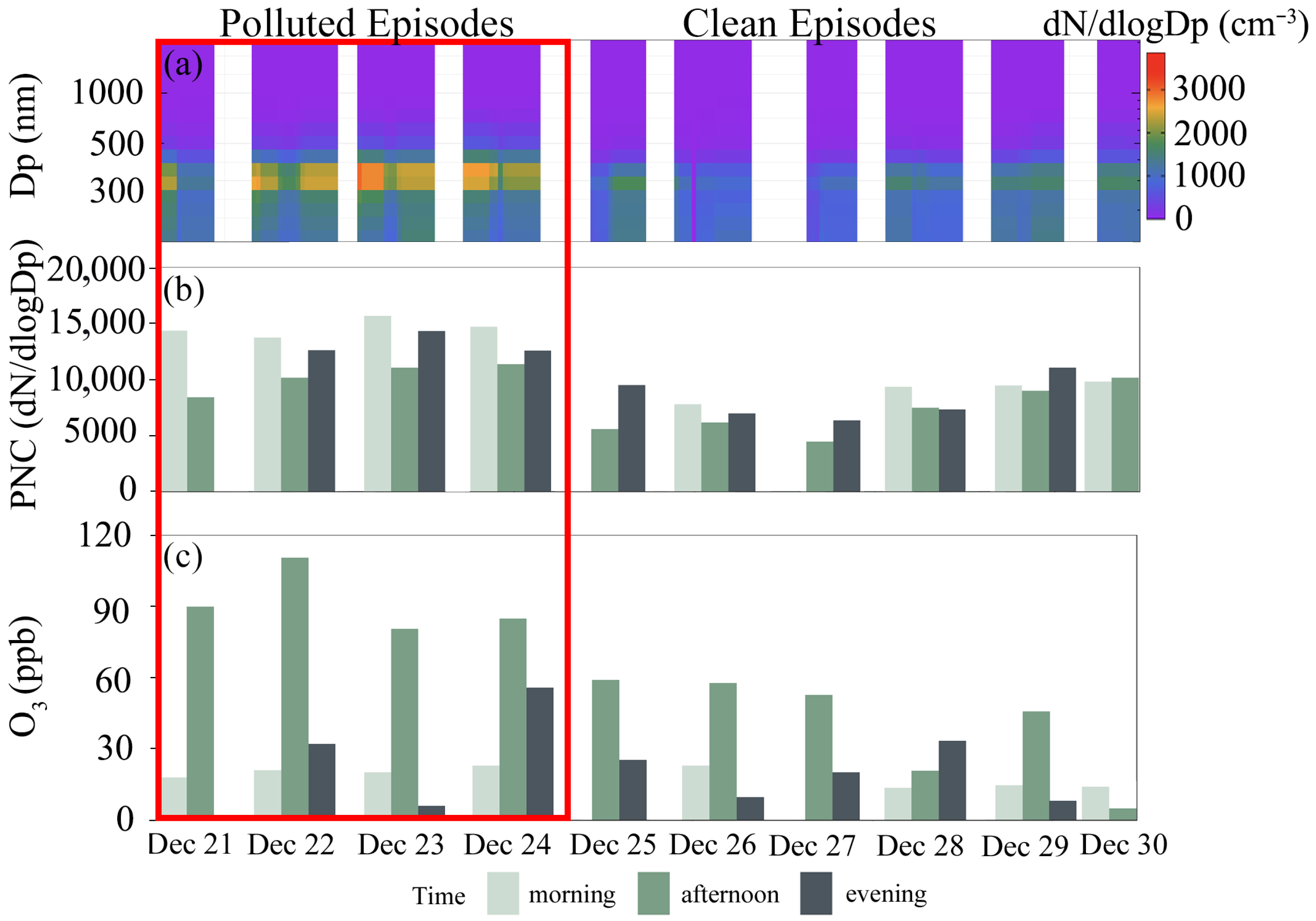
Figure 3 summarizes the particle number size distribution, total PNC, and O₃ concentrations measured during the mobile observation. As shown in Figure 3a, the majority of atmospheric particles were observed within the 200–400 nm diameter range, accounting for 92.03–98.15% of the total particles. On the morning of 25 December, a short-term precipitation event occurred that helped to remove particles with diameters ranging from 0.1–10 μm, especially those with diameters ranging from 0.1–0.5 μm. The hourly average total PNC ranged from 4291 to 16,342 dN/dlogdp (cm⁻³), as shown in Figure 3b. During the polluted episodes, the hourly average total PNC ranged from 7968 to 16,342 cm⁻³, whereas during the clean episodes, it ranged from 4291 to 11,040 cm⁻³. During the polluted period, the total PNC increased to approximately 10,000 cm⁻³, which may be attributed to various factors, such as the occurrence of inversion layers, atmospheric stability, and ground-level source emissions [53]. The average total PNC during the polluted episodes was 14,587 cm⁻³ in the morning, 10,244 cm⁻³ in the afternoon, and 13,140 cm⁻³ in the evening. Conversely, on 25 December, precipitation acted as a wet scavenger, reducing the PNC and thereby reducing the disparity between the total PNC. The average total PNCs during clean episodes are 9095 cm⁻³ in the morning, 8564 cm⁻³ in the afternoon, and 8243 cm⁻³ in the evening. Figure 3b indicates that the total PNC in the morning is generally greater than that in the afternoon and evening. Figure 3 summarizes the particle number size distribution, total PNC, and O₃ concentrations measured during the mobile observation. On the basis of the analysis shown in Figure 3c, the pattern of O₃ concentrations differs from that of the PNC. During the polluted episodes, the average O₃ concentration was 20.5 ppb in the morning, whereas it was 91.2 ppb in the afternoon and 31 ppb in the evening. During the clean episodes, the average O₃ concentration in the afternoon was approximately 56.5 ppb. Conversely, during clean episodes that are characterized by overcast and rainy conditions, the limited sunlight intensity results in low O₃ concentrations, even during the day.

Fixed station observations and mobile observations provide a comprehensive picture: while fixed stations offer continuous and meteorological data, mobile data capture particle size dynamics and spatial variability, revealing how local atmospheric structure and microclimatic events influence pollution patterns across time and space.

3.2. Correlations of Various Parameters

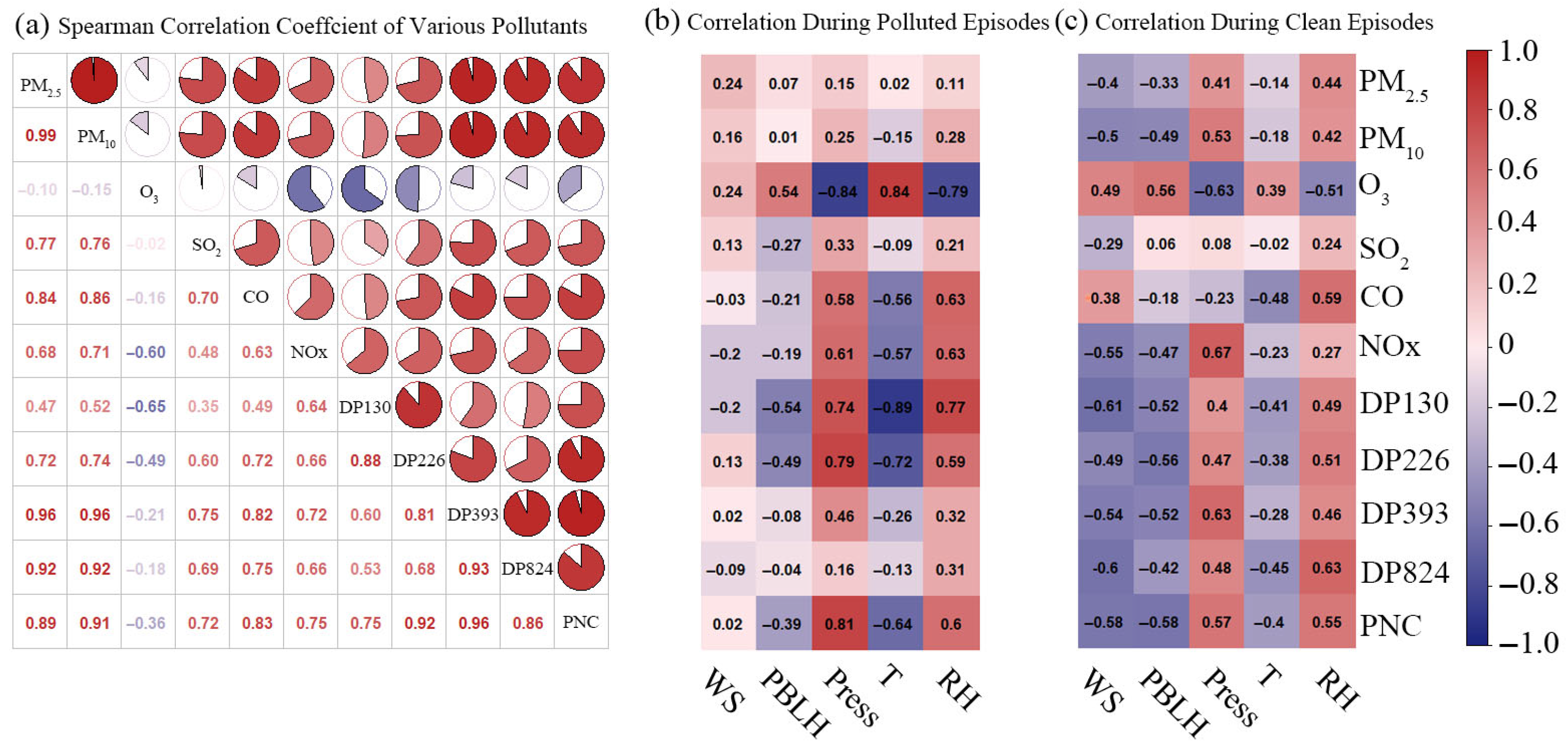
The relationships between meteorological variables (wind speed, PBLH, pressure, temperature, and RH) and pollutants were examined using Spearman correlation analysis at the 5% significance level (Figure 4). As shown in Figure 4a, PM_2.5 was positively correlated with several co-pollutants, especially SO₂ (r = 0.77), CO (r = 0.84) and NOx (r = 0.68), indicating the synchronous accumulation of particulate pollutants and combustion-related gases during winter. Among the particle size bins, particles around 400 nm showed the strongest correlations with SO₂ and NOx, with coefficients of 0.75 and 0.72, respectively. In contrast, O₃ showed negative correlations with particulate pollutants, particularly NOx (r = −0.6) and 130 nm particles (r = −0.65). Overall, these results indicate that particulate pollutants and combustion-related gaseous pollutants tended to increase simultaneously during the winter observation period, whereas O₃ exhibited a different variation pattern. In winter, high levels of PM_2.5 suppress O₃ formation by reducing solar radiation and scavenging reactive radicals [54], thereby slowing photochemical reactions. The negative correlation between NOx and O₃ concentrations is primarily due to the role of NOx as a precursor in ozone formation [55], where it undergoes a series of photochemical reactions that contribute to secondary particulate matter formation, which then becomes a component of PM_2.5. Under sufficient conditions, NOx underwent photochemical reactions, resulting in a negative correlation with O₃ concentrations. PM_2.5 showed a weak negative correlation with the O₃ concentration, which corroborated previous research findings [56].

Figure 4b,c illustrates the correlations between meteorological elements and various pollutants during polluted and clean episodes. A comparison revealed that the influence of wind speed was the opposite between these two episodes: during polluted episodes, wind speed demonstrated a weak correlation (−0.2 < r < 0.24), whereas during clean episodes, it showed a strong negative correlation with pollutants, except for O₃, where r = 0.24. Owing to the basin terrain, weak winds drove the transmission of particles, along with the mixing and aging of these particles. During clean episodes, as the wind speed increased and particulate matter aged, the particle concentrations further decreased. The O₃ and its precursors were delivered by the wind and were positively correlated with the wind speed. During the polluted episodes, no significant correlation was detected between the PBLH and the PM_2.5 concentration. However, during the clean episodes, a negative correlation was found between the PBLH and the particle concentration. Wind speed and PBLH generally reduce PM_2.5 concentrations by promoting dispersion and vertical mixing [57]. Increased wind speed can indirectly increase O₃ levels by diluting PM_2.5 and weakening its inhibitory effects [58]. Overall, these results suggest that winter PM enhancement was jointly influenced by co-emitted pollutants and episode-dependent meteorological conditions, which is consistent with the spatial heterogeneity observed along different routes and urban functional areas. When analyzing the PNC, a strong negative correlation with the smaller particle sizes (especially DP130 and DP226) is observed during polluted episodes, which suggests that larger particles may dominate during higher pollution periods, possibly due to aerosol aging and coagulation processes. During periods of high pollution, the lower wind speeds and reduced boundary layer height may limit the dispersion of pollutants, leading to higher concentrations. In contrast, during clean episodes, increased wind speeds and higher PBLH likely contribute to the dilution and removal of pollutants from the atmosphere, which is reflected in the weaker correlations observed in Figure 4c. The positive correlation observed in clean episodes also suggests that ozone may play a role in modifying particulate dynamics in environments with lower pollution levels. This could indicate that in cleaner conditions, O₃ is less likely to be consumed by particles, allowing for greater accumulation of both O₃ and particles, particularly in areas where local sources contribute to both.

These correlation patterns, when interpreted together with the mobile observations, suggest that the enhancement of PM_2.5 under winter pollution-favorable conditions was not spatially uniform, but instead varied substantially among different routes and urban functional areas.

3.3. Mobile Observation

The association between stagnant meteorological conditions and pollution accumulation is well established in urban atmospheric studies. Therefore, the main contribution of the present work does not lie in reconfirming this general relationship. Instead, the added value of the mobile observation is its ability to reveal fine-scale spatial heterogeneity within the city under the same winter pollution background. The results show that pollutant concentrations were not uniformly distributed, but varied substantially among routes and urban functional areas, indicating that local emissions, near-road environments, and urban surface characteristics play an important role in shaping intra-urban pollution patterns.

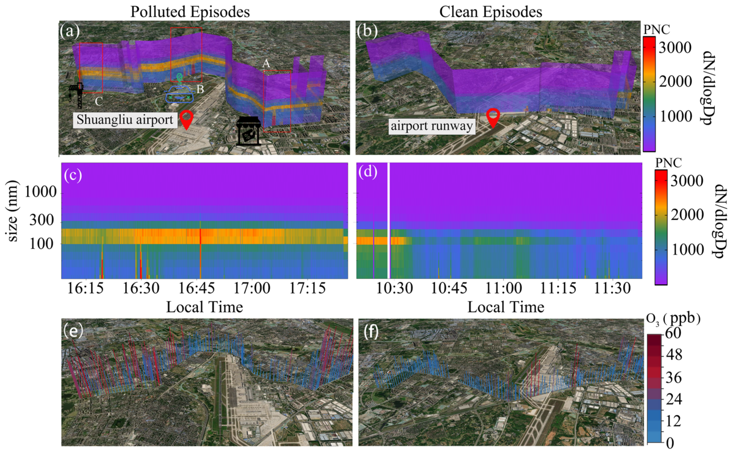
Figure 5a shows the time series of the particle size distributions and O₃ concentrations that were obtained via mobile observations on 23 December 2022. The bar height indicates the concentration color plot in all figures. There are 3 obvious locations indicating higher PNCs, especially those for fine particles (particle diameters less than 300 nm), which exceed 3000 cm⁻³. Point A is located next to a shopping mall. On 23 December, which was a holiday, there was an increased number of vehicles due to students gathering from nearby schools. Point B is an area with numerous car dealerships, including many high-emission trucks. Diesel fuels inefficiently and emits harmful chemical components, such as sulfides, carbon compounds, and nitrogen oxides, into the environment [59]. These locations release large amounts of aerosol precursors, and when coupled with strong photochemical reactions during the afternoon, PNC rapidly increases. Point C is located near a nearby construction site and can emit copious quantities of aerosol particles, leading to an increase in PNC. Therefore, human activities have had a significant impact on the distribution of PNC on this day.

Figure 5b shows the time series for the particle size spectrum for the vehicle on 26 December 2022, from 10:15 to 11:45. Compared with those during polluted episodes, the particle sizes in all the size segments obviously decreased. The PNC in the size range of 300–400 nm was greater by 800–1500 cm⁻³ than those in the other time periods during clean episodes, reaching 2800 cm⁻³. The time series plot and geographical characteristics revealed that the sampling site was located beneath an airport expressway that is surrounded by tall buildings and has low vegetation coverage, which indicates an urban street canyon environment [60]. Furthermore, shortly after the morning rush hour, there was a notable presence of locally generated pollutants, as the aerosol particles that were emitted by many vehicles were not adequately dispersed. The average PNC recorded during the sampling period was 11,192 cm⁻³. Upon reaching the park, the average total PNC was 8737 cm⁻³, whereas in the nonpark areas, the value was 7460 cm⁻³, indicating a 17.11% ±1% increase near the park. At point A, there was no apparent emission of fine particles during clean episodes. In subsequent mobile observations, it was evident that during working hours on weekdays, there was a significant reduction in fine particle emissions on the streets, indicating that anthropogenic factors played a predominant role in fine particle emissions on these main streets. Owing to traffic congestion or traveling alongside high-emission vehicles, the PNCs increased, which was referred to as a PNSD (particle number size distribution) surge event. The occurrence of such events was reflected in the spatial and temporal distributions obtained from multiple mobile observations, and the points that correspond to these events could be categorized as instances where anthropogenic factors contribute to increases in fine PNC. Additionally, high concentrations of PM_2.5 can inhibit photolytic reactions [61].

Figure 5c,d present the size-resolved PNSD corresponding to the mobile observations shown in Figure 5a,b, respectively. The PNSD information was mapped onto the mobile routes to construct the spatial distributions in Figure 5a,b. In the polluted case, particle number concentrations were mainly enhanced in the 100–300 nm size range, with the highest values around 100–200 nm, and the high-concentration band persisted for much of the observation period. In contrast, the clean case showed much lower PNSD levels and a clearly weakened high-concentration band. These results suggest that the spatial enhancement of PNC in the polluted case was primarily associated with sustained accumulation-mode particle enrichment.

Figure 5e shows that the temporal and spatial O₃ distributions clearly reveal two peaks in the O₃ concentrations near the airport runway, reaching 55.8 and 58.8 ppb respectively. There was a significant presence of transportation vehicles, including trucks, near airports. By combining the data obtained from the hand-held meteorological stations with the spatiotemporal distribution map of the O₃ concentrations (as indicated in S2), it is possible to infer the pollutant sources on the basis of meteorological variables such as temperature, RH, radiation intensity, and ultraviolet radiation. A spatial and temporal distribution map of the O₃ concentrations revealed higher O₃ concentrations at the park and at the starting point. This could be attributed to the high temperatures and intense sunlight during departure, which promote the photochemical reactions of O₃ precursors and result in elevated O₃ concentrations. The increased O₃ concentrations around the park may be attributed to the abundant emissions of VOCs from vegetation under sufficient sunlight [62]. Additionally, activities such as aircraft takeoff [63], soil [62], and refueling also contribute to ozone precursor emissions and further promote O₃ formation.

The observational framework adopted in this study can serve as a practical supplement to conventional fixed-site monitoring. By combining short-term intensive mobile measurements with synchronous fixed-site observations, it is possible to identify fine-scale pollution hotspots and resolve spatial heterogeneity more effectively (more Spatial distribution map shown in Figures S9 and S10). Moreover, depending on the monitoring objective, available resources, and operational conditions, this framework can also be adapted for repeated observation or longer-term applications.

3.4. PCA Results

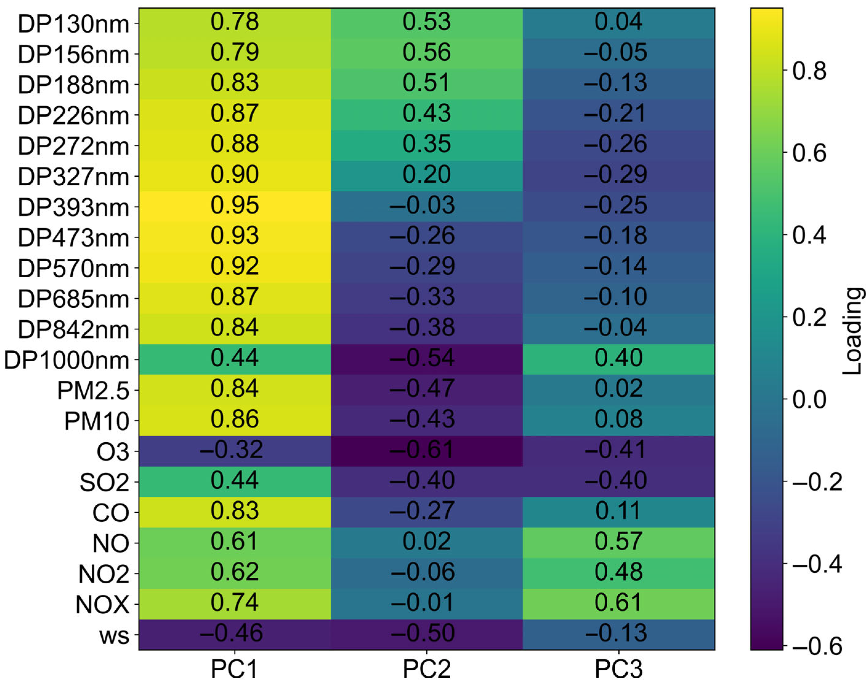
PCA was performed on the standardized hourly dataset (n = 224; 21 variables) to explore the major covariance structures among particle number concentrations in different size bins, gaseous pollutants, particulate matter, and meteorological conditions. The dataset was suitable for PCA, as indicated by a Kaiser–Meyer–Olkin value of 0.788 and a highly significant Bartlett’s test of sphericity (p < 0.001). Three principal components with eigenvalues > 1 were retained, explaining 82.66% of the total variance, with PC1, PC2, and PC3 accounting for 59.13%, 15.05%, and 8.48%, respectively (as shown in Figures S4 and S5). Figure 6 shows that PC1 showed strong positive loadings for most particle size bins, particularly 226–842 nm, as well as PM_2.5 and PM₁₀, together with a negative loading for wind speed, indicating that this component primarily represented a regional accumulation pattern under relatively stagnant atmospheric conditions. PC2 was characterized by positive loadings for O₃ wind speed, PM, and the 1000 nm size bin, but negative loadings for the smaller particle size bins (130–226 nm), suggesting a contrast between oxidizing and more ventilated conditions and periods dominated by smaller particles. PC3 was dominated by strong positive loadings of NO, NO₂, and NOx, accompanied by a negative loading of O₃, which likely reflected a fresh combustion-related influence associated with ozone titration. Overall, the PCA results suggest that the variability of the measured pollutants was mainly governed by three processes, namely pollution accumulation under weak dispersion, changes in oxidation and ventilation conditions, and primary NO-related emissions.

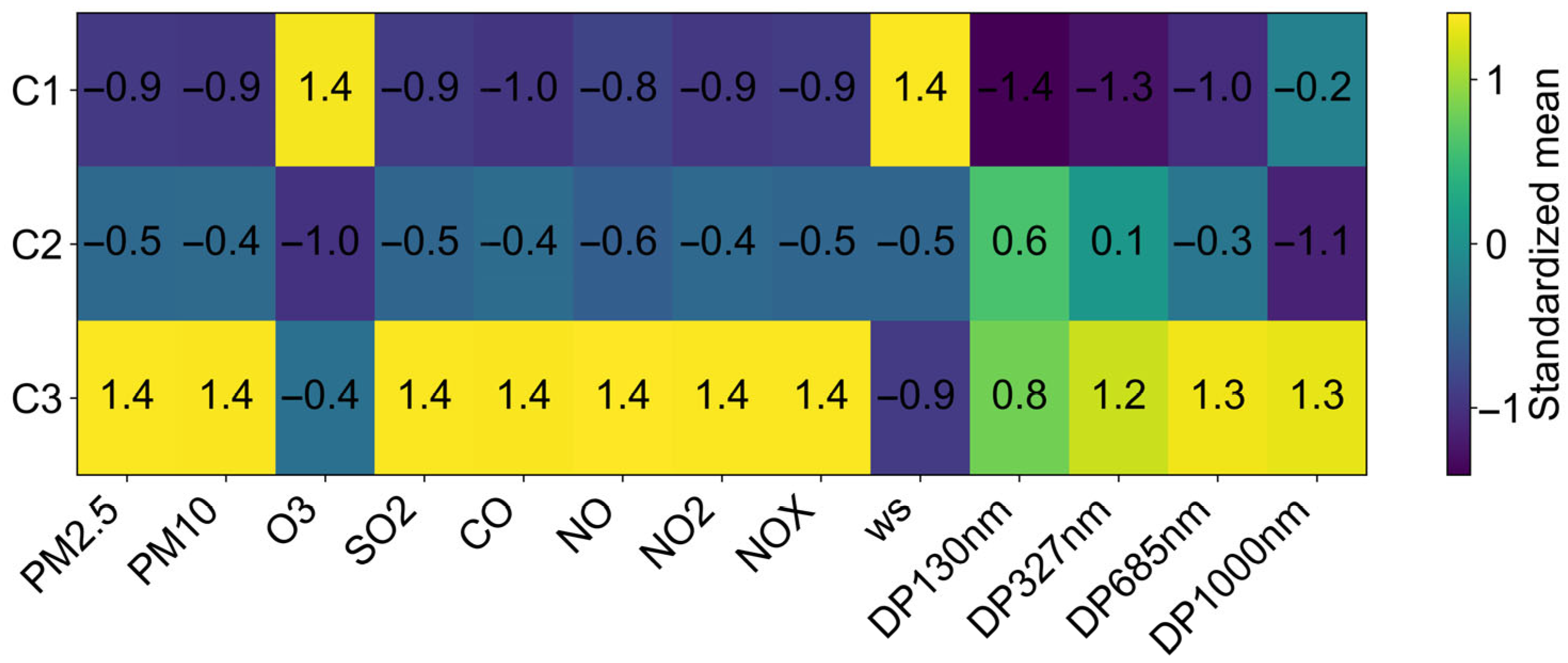
To further classify the dominant aerosol pollution regimes, k-means clustering was applied to the scores of the first three principal components, which together explained 82.66% of the total variance (as shown in Figure S6). Shown in Figure S7, although the silhouette analysis indicated that the two-cluster solution yielded the highest coefficient (0.410), the three-cluster solution (silhouette = 0.364) provided a more physically interpretable separation of atmospheric conditions and was therefore adopted for subsequent analysis. Figure 7 shows that the 224 matched hourly observations were classified into three regimes: Cluster 1 (n = 77), Cluster 2 (n = 89), and Cluster 3 (n = 58). Cluster 1 represented a relatively clean and ventilated regime, characterized by the lowest PM_2.5 (46.4 μg m⁻³), PM₁₀ (62.7 μg m⁻³), CO (0.37), NOx (39.9), and particle number concentrations across most selected size bins, together with the highest WS (1.03 m s⁻¹). In contrast, Cluster 3 corresponded to a heavily polluted accumulation regime, with substantially elevated PM_2.5 (149.4 μg m⁻³), PM₁₀ (189.9 μg m⁻³), CO (1.39), NO (33.7), NO₂ (67.4), NOx (119.0), and markedly enhanced particle number concentrations, especially in the 327, 685, and 1000 nm size ranges, while WS remained comparatively low (0.65 m s⁻¹). Cluster 2 exhibited intermediate pollutant levels, with PM_2.5, PM₁₀, CO, and NOx between those of Clusters 1 and 3, indicating a transitional accumulation regime under weaker dispersion conditions than Cluster 1. Notably, O₃ was highest in Cluster 1 and lowest in Cluster 2, whereas Cluster 3 showed moderate O₃ despite very high NOx, suggesting that the oxidation environment varied substantially across the identified regimes and may have been influenced by both ventilation and local titration effects. Overall, the PCA-based clustering effectively separated the observations into clean/ventilated, intermediate accumulation, and heavy accumulation conditions, indicating that aerosol variability during the study period was governed primarily by changes in dispersion conditions and the co-evolution of particulate and gaseous pollutants.

3.5. Backward Trajectory Analysis

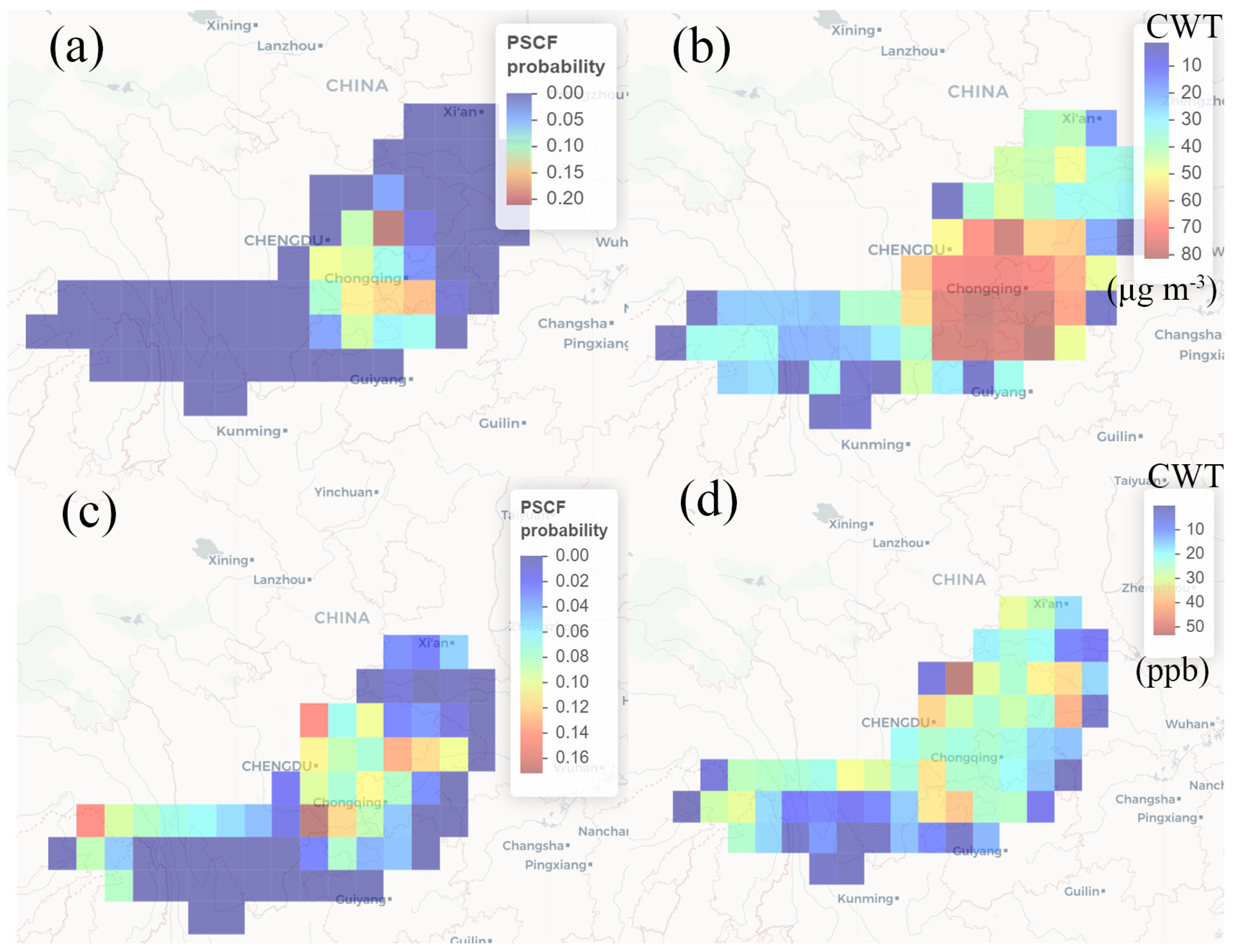
Figure 8a shows the substantial impact of the pollution sources located southeast and west of Chengdu on the PM_2.5 levels in December 2022, and Figure 8b shows the results of PSCF in December 2022. The CWT and PSCF were carried out to identify the potential source regions of PM_2.5 and their influence on the PM_2.5 levels at Baihe station. December was the primary month when PM_2.5 pollution occurred, with the pollutants originating primarily from local emissions and from some industrial cities in East China. These cities contributed more than 70 μg m⁻³ of PM_2.5. The southeastern contribution can be largely attributed to emissions originating from Chongqing and Guizhou Provinces. These areas are characterized by the notable presence of industrial factories and the annual occurrence of agricultural residue burning activities. The pollutants that were emitted from these anthropogenic sources were transported to the Sichuan Basin by east winds. Furthermore, the western contribution primarily stemmed from the Tibetan Plateau, which still contributed approximately 50 μg m⁻³ of PM_2.5. The Tibetan Plateau has a sparse human population, and anthropogenic emissions play a minor role in its pollution contribution [64]. Instead, the plateau acted as a receptor for pollutant accumulation due to natural disasters and anthropogenic activities, such as the burning of agricultural residues in South Asia and Southeast Asia. Under the influence of a monsoon climate, atmospheric pollutants accumulate at the foothills of the Himalayas [65]. These pollutants are then transported to the Tibetan Plateau through upward and horizontal airflows and eventually reach the Sichuan Basin. Minor contributions of pollutants were also observed in the northwest. This contribution was attributed to sources in China’s Xinjiang Province, as well as the border regions of Kazakhstan and Russia. In December 2022 (shown in Figure 8b), Neijiang city was identified as the main source of PM_2.5 transport, with a contribution probability of 0.21. Pollutants also originated from the eastern and southern cities of Chengdu, with contribution probabilities ranging from 0.05–0.2.

Figure 8c shows the CWT of O₃ concentrations. The map highlights several regions with varying levels of pollutant contributions, with the highest concentrations (up to 50 ppb) appearing in areas located primarily east of the Baihe site, encompassing cities such as Deyang and Nanchong city. Locally generated O₃ concentrations constitute a substantial proportion. Figure 8d shows the PSCF for December 2022, revealing a wide range of O₃ sources. The northern cities, such as Beichuan and Mao County, had a contribution probability of 0.15, the eastern cities, such as Dazhou and Neijiang City, had a contribution probability of 0.13, the southern cities, such as Yibin City, had a contribution probability of 0.17, and the western region (Qinghai—Tibet Plateau) had a contribution probability ranging from 0.07–0.15. Combining the CWT and PSCF analyses, the results indicated that in December, the source of O₃ had the same variation rules as those of PM_2.5. The main source of O₃ was from eastern cities, which are industrial cities. Both the CWT and PSCF analyses point to a consistent pattern, identifying the northeastern regions, including major urban and industrial centers, as significant contributors to the observed pollution at the receptor site. The strong alignment between the high-concentration areas in the CWT map and the high-probability regions in the PSCF map strengthens the hypothesis that these regions were key source areas. The presence of moderate contributions from other directions, as indicated in the CWT map, suggested that while the southeastern and eastern regions were primary sources, other regions may also play a role, albeit to a lesser extent.

4. Conclusions

This study used mobile monitoring to characterize the fine-scale spatial variability of urban air pollution during a winter intensive observation period in Chengdu. Compared with conventional fixed-site observations, the mobile approach provided a clearer picture of intra-urban pollution heterogeneity by resolving localized concentration gradients, route-scale differences, and pollution hotspots that are difficult to capture with routine monitoring alone.

From a local pollution perspective, an analysis of the collected data revealed average hourly PNCs ranging from 4290 to 16,342 cm⁻³. DP smaller than 0.5 μm accounted for 92% to 98% of the total. During the polluted episode (from 21–24 December), the average hourly PNCs ranged from 7967 to 16,342 cm⁻³, while during the clean episodes (from 25–30 December), they ranged from 4290 to 11,039·cm⁻³. The O₃ concentrations ranged from 4 to 117 ppb. Quantitative analyses further supported these findings. The first three principal components explained 82.7% of the total variance, indicating that the major variability in pollutants and meteorological conditions could be effectively captured by a limited number of dominant factors. Cluster analysis identified three pollution regimes among 224 samples, namely clean/ventilated (34.4%), intermediate accumulation (39.7%), and heavy accumulation (25.9%). The corresponding mean PM_2.5 concentrations were 46.4, 67.1, and 149.4 μg m⁻³, respectively, showing that PM_2.5 levels under heavy accumulation were about 3.2 times those under clean/ventilated conditions. Correlation analysis also revealed strong associations between PM_2.5 and PM₁₀ (r = 0.99), SO₂ (r = 0.77), and NOx (r = 0.68), whereas O₃ showed negative correlations with fine particles, with the strongest relationship observed for 130 nm particles (r = −0.65).

A key finding is that urban pollution hotspots were not uniform in space or time. Some hotspots showed relatively persistent spatial occurrence, suggesting the influence of stable local emissions and urban environmental conditions, whereas others appeared only intermittently, reflecting the importance of transient traffic activity, short-term emission disturbances, and local dispersion conditions. This ability to distinguish persistent from occasional hotspots represents an important contribution of the mobile monitoring approach and provides added value beyond confirming the well-established role of meteorology in pollution accumulation.

Overall, these results demonstrate that short-term intensive mobile monitoring, when combined with fixed-site observations, provides a practical and cost-effective approach for identifying urban pollution hotspots, characterizing pollution regimes, and interpreting the combined effects of emissions and meteorological conditions. This framework can support rapid pollution screening and targeted urban air-quality management, and it may also be extended to repeated campaigns or longer-term applications depending on monitoring objectives and available resources. The present study is nevertheless limited by its short winter observation period and the lack of quantitative precipitation data, which should be addressed in future work.

References

1. Chen, P.C.; Mou, C.H.; Chen, C.W.; Hsieh, D.P.H.; Tsai, S.P.; Wei, C.C.; Sung, F.C. Roles of Ambient Temperature and PM(2.5) on Childhood Acute Bronchitis and Bronchiolitis from Viral Infection. Viruses 2022, 14, 1932. [Google Scholar] [CrossRef]
2. Shou, Y.; Huang, Y.; Zhu, X.; Liu, C.; Hu, Y.; Wang, H. A review of the possible associations between ambient PM2.5 exposures and the development of Alzheimer’s disease. Ecotoxicol. Environ. Saf. 2019, 174, 344–352. [Google Scholar] [CrossRef]
3. Holm, S.M.; Balmes, J.R. Systematic Review of Ozone Effects on Human Lung Function, 2013 Through 2020. Chest 2022, 161, 190–201. [Google Scholar] [CrossRef]
4. Sun, Y.; Zhuang, G.; Tang, A.; Wang, Y.; An, Z. Chemical Characteristics of PM2.5 and PM10 in Haze−Fog Episodes in Beijing. Environ. Sci. Technol. 2006, 40, 3148–3155. [Google Scholar] [CrossRef]
5. Chen, Z.; Chen, D.; Zhao, C.; Kwan, M.P.; Cai, J.; Zhuang, Y.; Zhao, B.; Wang, X.; Chen, B.; Yang, J.; et al. Influence of meteorological conditions on PM2.5 concentrations across China: A review of methodology and mechanism. Environ. Int. 2020, 139, 105558. [Google Scholar] [CrossRef]
6. Hu, J.; Zhao, T.; Liu, J.; Cao, L.; Wang, C.; Li, Y.; Shi, C.; Tan, C.; Sun, X.; Shu, Z.; et al. Exploring the ozone pollution over the western Sichuan Basin, Southwest China: The impact of diurnal change in mountain-plains solenoid. Sci. Total Environ. 2022, 839, 156264. [Google Scholar] [CrossRef]
7. Guttikunda, S.K.; Goel, R.; Pant, P. Nature of air pollution, emission sources, and management in the Indian cities. Atmos. Environ. 2014, 95, 501–510. [Google Scholar] [CrossRef]
8. Xing, J.; Pleim, J.; Mathur, R.; Pouliot, G.; Hogrefe, C.; Gan, C.M.; Wei, C. Historical gaseous and primary aerosol emissions in the United States from 1990 to 2010. Atmos. Chem. Phys. 2013, 13, 7531–7549. [Google Scholar] [CrossRef]
9. Liang, C.-S.; Wu, H.; Li, H.-Y.; Zhang, Q.; Li, Z.; He, K.-B. Efficient data preprocessing, episode classification, and source apportionment of particle number concentrations. Sci. Total Environ. 2020, 744, 140923. [Google Scholar] [CrossRef] [PubMed]
10. Song, Y.; Zhang, Y.; Xie, S.; Zeng, L.; Zheng, M.; Salmon, L.G.; Shao, M.; Slanina, S. Source apportionment of PM2.5 in Beijing by positive matrix factorization. Atmos. Environ. 2006, 40, 1526–1537. [Google Scholar] [CrossRef]
11. Li, Y.; Chen, Q.; Zhao, H.; Wang, L.; Tao, R. Variations in PM10, PM2.5 and PM1.0 in an Urban Area of the Sichuan Basin and Their Relation to Meteorological Factors. Atmosphere 2015, 6, 150–163. [Google Scholar] [CrossRef]
12. Wang, H.; Shi, G.; Tian, M.; Zhang, L.; Chen, Y.; Yang, F.; Cao, X. Aerosol optical properties and chemical composition apportionment in Sichuan Basin, China. Sci. Total Environ. 2017, 577, 245–257. [Google Scholar] [CrossRef] [PubMed]
13. Li, K.; Chen, L.; Ying, F.; White, S.J.; Jang, C.; Wu, X.; Gao, X.; Hong, S.; Shen, J.; Azzi, M.; et al. Meteorological and chemical impacts on ozone formation: A case study in Hangzhou, China. Atmos. Res. 2017, 196, 40–52. [Google Scholar] [CrossRef]
14. Cai, J.; Chu, B.; Yao, L.; Yan, C.; Heikkinen, L.M.; Zheng, F.; Li, C.; Fan, X.; Zhang, S.; Yang, D.; et al. Size-segregated particle number and mass concentrations from different emission sources in urban Beijing. Atmos. Chem. Phys. 2020, 20, 12721–12740. [Google Scholar] [CrossRef]
15. Ogulei, D.; Hopke, P.K.; Chalupa, D.C.; Utell, M.J. Modeling Source Contributions to Submicron Particle Number Concentrations Measured in Rochester, New York. Aerosol Sci. Technol. 2007, 41, 179–201. [Google Scholar] [CrossRef]
16. Mohan, V.; Kumar Soni, V.; Kumar Mishra, R. Analysing the impact of day-night road traffic variation on ultrafine particle number size distribution and concentration at an urban site in the megacity Delhi. Atmos. Pollut. Res. 2024, 15, 102065. [Google Scholar] [CrossRef]
17. Wåhlin, P.; Palmgren, F.; Van Dingenen, R. Experimental studies of ultrafine particles in streets and the relationship to traffic. Atmos. Environ. 2001, 35, S63–S69. [Google Scholar] [CrossRef]
18. Al-Dabbous, A.N.; Kumar, P. Source apportionment of airborne nanoparticles in a Middle Eastern city using positive matrix factorization. Environ. Sci. Process. Impacts 2015, 17, 802–812. [Google Scholar] [CrossRef] [PubMed]
19. Kim, N.G.; Jeong, S.B.; Jin, H.C.; Lee, J.; Kim, K.H.; Kim, S.; Park, Y.; Choi, W.; Kwak, K.-H.; Lee, H.; et al. Spatial and PMF analysis of particle size distributions simultaneously measured at four locations at the roadside of highways. Sci. Total Environ. 2023, 893, 164892. [Google Scholar] [CrossRef]
20. Perrone, M.G.; Vratolis, S.; Georgieva, E.; Török, S.; Šega, K.; Veleva, B.; Osán, J.; Bešlić, I.; Kertész, Z.; Pernigotti, D.; et al. Sources and geographic origin of particulate matter in urban areas of the Danube macro-region: The cases of Zagreb (Croatia), Budapest (Hungary) and Sofia (Bulgaria). Sci. Total Environ. 2018, 619–620, 1515–1529. [Google Scholar] [CrossRef]
21. Price, H.D.; Arthur, R.; BéruBé, K.A.; Jones, T.P. Linking particle number concentration (PNC), meteorology and traffic variables in a UK street canyon. Atmos. Res. 2014, 147–148, 133–144. [Google Scholar] [CrossRef]
22. Kumari, S.; Jain, M.A.-O.; Elumalai, S.A.-O. Assessment of Pollution and Health Risks of Heavy Metals in Particulate Matter and Road Dust Along the Road Network of Dhanbad, India. J. Health Pollut. 2021, 11, 210305. [Google Scholar] [CrossRef]
23. Belarbi, N.; Belamri, M.; Dahmani, B.; Benamar, M. Road traffic and PM10, PM2.5 emission at an urban area in Algeria: Identification and statistical analysis. Pollution 2020, 6, 651–660. [Google Scholar]
24. Edussuriya, P.; Chan, A.; Ye, A. Urban morphology and air quality in dense residential environments in Hong Kong. Part I: District-level analysis. Atmos. Environ. 2011, 45, 4789–4803. [Google Scholar] [CrossRef]
25. Fang, C.; Qiu, J.; Li, J.; Wang, J. Analysis of the meteorological impact on PM2.5 pollution in Changchun based on KZ filter and WRF-CMAQ. Atmos. Environ. 2022, 271, 118924. [Google Scholar] [CrossRef]
26. Wang, R.; Tie, X.; Li, G.; Zhao, S.; Long, X.; Johansson, L.; An, Z. Effect of ship emissions on O3 in the Yangtze River Delta region of China: Analysis of WRF-Chem modeling. Sci. Total Environ. 2019, 683, 360–370. [Google Scholar] [CrossRef]
27. Zhang, Z.Y.; Wong, M.S.; Lee, K.H. Estimation of potential source regions of PM 2.5 in Beijing using backward trajectories. Atmos. Pollut. Res. 2015, 6, 173–177. [Google Scholar] [CrossRef]
28. He, J.; Yu, Y.; Liu, N.; Zhao, S. Numerical model-based relationship between meteorological conditions and air quality and its implication for urban air quality management. Int. J. Environ. Pollut. 2013, 53, 265–286. [Google Scholar] [CrossRef]
29. Tsin, P.K.; Knudby, A.; Krayenhoff, E.S.; Ho, H.C.; Brauer, M.; Henderson, S.B. Microscale mobile monitoring of urban air temperature. Urban Clim. 2016, 18, 58–72. [Google Scholar] [CrossRef]
30. Van den Bossche, J.; Peters, J.; Verwaeren, J.; Botteldooren, D.; Theunis, J.; De Baets, B. Mobile monitoring for mapping spatial variation in urban air quality: Development and validation of a methodology based on an extensive dataset. Atmos. Environ. 2015, 105, 148–161. [Google Scholar] [CrossRef]
31. Yu, C.H.; Fan, Z.; Lioy, P.J.; Baptista, A.; Greenberg, M.; Laumbach, R.J. A novel mobile monitoring approach to characterize spatial and temporal variation in traffic-related air pollutants in an urban community. Atmos. Environ. 2016, 141, 161–173. [Google Scholar] [CrossRef]
32. Chai, W.; Tang, G.; Wang, S.; Wang, T.; Zheng, H.; Hpi, Y. Analysis of an Air Pollution of Dust Process Using Mobile Lidar over Beijing-Tianjin-Hebei Area. Environ. Monit. China 2019, 35, 138–145. [Google Scholar] [CrossRef]
33. Liu, X.; Huang, J.; Wang, Y.; Zhang, L. Study on mobile monitoring for finding urban small—Scale air—Pollution hotspots. Environ. Sustain. Dev. 2019, 44, 66–69. [Google Scholar] [CrossRef]
34. Si, S.; Xu, H.; Zhang, Z.; Gao, J.; Qin, X. Study on the Monitoring System of Atmospheric Particulate Matter in Urban Taxi: A Case Study of Jinan City, Shandong Province. Environ. Prot. 2020, 48, 54–57. [Google Scholar] [CrossRef]
35. Wallace, J.; Corr, D.; Deluca, P.; Kanaroglou, P.; McCarry, B. Mobile monitoring of air pollution in cities: The case of Hamilton, Ontario, Canada. J. Environ. Monit. 2009, 11, 998–1003. [Google Scholar] [CrossRef]
36. Padro-Martinez, L.T.; Patton, A.P.; Trull, J.B.; Zamore, W.; Brugge, D.; Durant, J.L. Mobile monitoring of particle number concentration and other traffic-related air pollutants in a near-highway neighborhood over the course of a year. Atmos. Environ. 2012, 61, 253–264. [Google Scholar] [CrossRef]
37. Li, Z.; Li, C.; Ye, X.; Fu, H.; Wang, L.; Yang, X.; Wang, X.; Zhao, Z.; Kan, H.; Mellouki, A.; et al. Air quality in the middle and lower reaches of the Yangtze River channel: A cruise campaign. Atmos. Chem. Phys. 2018, 18, 14445–14464. [Google Scholar] [CrossRef]
38. Wang, H.; Gao, Y.; Jing, S.-a.; Lou, S.; Hu, Q.; An, J.; Wu, Y.; Gao, W.; Zhu, L.; Huang, C. Characterization of Volatile Organic Compounds (VOCs) Using Mobile Monitoring Around the Industrial Parks in the Yangzte River Delta Region of China. Environ. Sci. 2021, 42, 1298–1305. [Google Scholar] [CrossRef]
39. Li, L.; Yang, L. Effects of driving restrictions on air quality and housing prices: Evidence from Chengdu, China. Transp. Res. Part A Policy Pract. 2023, 176, 103829. [Google Scholar] [CrossRef]
40. Song, M.; Liu, X.; Tan, Q.; Feng, M.; Qu, Y.; An, J.; Zhang, Y. Characteristics and formation mechanism of persistent extreme haze pollution events in Chengdu, southwestern China. Environ. Pollut. 2019, 251, 1–12. [Google Scholar] [CrossRef]
41. Shi, K.; Di, B.; Zhang, K.; Feng, C.; Svirchev, L. Detrended cross-correlation analysis of urban traffic congestion and NO2 concentrations in Chengdu. Transp. Res. Part D Transp. Environ. 2018, 61, 165–173. [Google Scholar] [CrossRef]
42. Todt, M.A.; Asher, E.; Hall, E.; Cullis, P.; Jordan, A.; Xiong, K.; Hurst, D.F.; Thornberry, T. Baseline Balloon Stratospheric Aerosol Profiles (B2SAP)—Systematic Measurements of Aerosol Number Density and Size. J. Geophys. Res. Atmos. 2023, 128, e2022JD038041. [Google Scholar] [CrossRef]
43. Wold, S.; Esbensen, K.; Geladi, P. Principal component analysis. Chemom. Intell. Lab. Syst. 1987, 2, 37–52. [Google Scholar] [CrossRef]
44. Greenacre, M.; Groenen, P.J.F.; Hastie, T.; D’Enza, A.I.; Markos, A.; Tuzhilina, E. Principal component analysis. Nat. Rev. Methods Primers 2022, 2, 100. [Google Scholar] [CrossRef] [PubMed]
45. Zhao, R.; Zhan, L.; Yao, M.; Yang, L. A geographically weighted regression model augmented by Geodetector analysis and principal component analysis for the spatial distribution of PM2.5. Sustain. Cities Soc. 2020, 56, 102106. [Google Scholar] [CrossRef]
46. Zheng, Y.; Che, H.; Yang, L.; Chen, J.; Wang, Y.; Xia, X.; Zhao, H.; Wang, H.; Wang, D.; Gui, K.; et al. Optical and radiative properties of aerosols during a severe haze episode over the North China Plain in December 2016. J. Meteorol. Res. 2018, 31, 1045–1061. [Google Scholar] [CrossRef]
47. Stohl, A. Trajectory statistics-A new method to establish source-receptor relationships of air pollutants and its application to the transport of particulate sulfate in Europe. Atmos. Environ. 1996, 30, 579–587. [Google Scholar] [CrossRef]
48. Manousakas, M.I.; Florou, K.; Pandis, S.N. Source Apportionment of Fine Organic and Inorganic Atmospheric Aerosol in an Urban Background Area in Greece. Atmosphere 2020, 11, 330. [Google Scholar] [CrossRef]
49. Han, Y.J.; Holsen, T.M.; Hopke, P.K.; Yi, S.M. Comparison between back-trajectory based modeling and Lagrangian backward dispersion Modeling for locating sources of reactive gaseous mercury. Environ. Sci. Technol. 2005, 39, 1715–1723. [Google Scholar]
50. Wu, J.-B.; Xu, J.; Pagowski, M.; Geng, F.; Gu, S.; Zhou, G.; Xie, Y.; Yu, Z. Modeling study of a severe aerosol pollution event in December 2013 over Shanghai China: An application of chemical data assimilation. Particuology 2015, 20, 41–51. [Google Scholar] [CrossRef]
51. You, T.; Wu, R.; Huang, G.; Fan, G. Regional meteorological patterns for heavy pollution events in Beijing. J. Meteorol. Res. 2017, 31, 597–611. [Google Scholar] [CrossRef]
52. Zhang, S.P.; Han, L.J.; Zhou, W.Q.; Zheng, X.X. Relationships between fine particulate matter (Pm2.5) and meteorological factors in winter at typical Chinese. Shengtai Xuebao 2016, 36, 7897–7907. [Google Scholar] [CrossRef]
53. Xiang, Y.; Zhang, T.; Liu, J.; Lv, L.; Dong, Y.; Chen, Z. Atmosphere boundary layer height and its effect on air pollutants in Beijing during winter heavy pollution. Atmos. Res. 2019, 215, 305–316. [Google Scholar] [CrossRef]
54. Gopikrishnan, G.P.; Westervelt, D.M.; Kuttippurath, J. Sensitivity of photochemical surface ozone formation regimes to emissions and meteorology in India. Atmos. Chem. Phys. 2026, 26, 1907–1929. [Google Scholar] [CrossRef]
55. Han, D.; Gao, C.; Li, Y.; Liu, H.; Cong, J.; Yu, X.; Wang, G. Potential in paleoclimate reconstruction of modern pollen assemblages from natural and human-induced vegetation along the Heilongjiang River basin, NE China. Sci. Total Environ. 2020, 745, 141121. [Google Scholar] [CrossRef]
56. Chu, B.; Ma, Q.; Liu, J.; Ma, J.; Zhang, P.; Chen, T.; Feng, Q.; Wang, C.; Yang, N.; Ma, H.; et al. Air Pollutant Correlations in China: Secondary Air Pollutant Responses to NOx and SO2 Control. Environ. Sci. Technol. Lett. 2020, 7, 695–700. [Google Scholar] [CrossRef]
57. Wang, J.; Han, J.; Li, T.; Wu, T.; Fang, C. Impact analysis of meteorological variables on PM(2.5) pollution in the most polluted cities in China. Heliyon 2023, 9, e17609. [Google Scholar] [CrossRef]
58. Ma, S.; Shao, M.; Zhang, Y.; Dai, Q.; Xie, M. Sensitivity of PM(2.5) and O(3) pollution episodes to meteorological factors over the North China Plain. Sci. Total Environ. 2021, 792, 148474. [Google Scholar] [CrossRef]
59. Reşitoğlu, İ.A.; Altinişik, K.; Keskin, A. The pollutant emissions from diesel-engine vehicles and exhaust aftertreatment systems. Clean Technol. Environ. Policy 2014, 17, 15–27. [Google Scholar] [CrossRef]
60. Hu, C.-B.; Zhang, F.; Gong, F.-Y.; Ratti, C.; Li, X. Classification and mapping of urban canyon geometry using Google Street View images and deep multitask learning. Build. Environ. 2020, 167, 106424. [Google Scholar] [CrossRef]
61. Wei, W.; Wang, Y.; Bai, H.; Wang, X.; Cheng, S.; Wang, L. Insights into atmospheric oxidation capacity and its impact on PM2.5 in megacity Beijing via volatile organic compounds measurements. Atmos. Res. 2021, 258, 105632. [Google Scholar] [CrossRef]
62. Yang, W.; Zhang, B.; Wu, Y.; Liu, S.; Kong, F.; Li, L. Effects of soil drought and nitrogen deposition on BVOC emissions and their O3 and SOA formation for Pinus thunbergii. Environ. Pollut. 2023, 316, 120693. [Google Scholar] [CrossRef]
63. Chen, M.; Li, S.; Yun, L.; Xu, Y.; Chen, D.; Lin, C.; Qiu, Z.; You, Y.; Liu, M.; Luo, Z.; et al. Characteristics of Volatile Organic Compounds Emitted from Airport Sources and Their Effects on Ozone Production. Toxics 2024, 12, 243. [Google Scholar] [CrossRef]
64. Yao, T. Tackling on environmental changes in Tibetan Plateau with focus on water, ecosystem and adaptation. Sci. Bull. 2019, 64, 417. [Google Scholar] [CrossRef]
65. Kang, S.; Zhang, Q.; Qian, Y.; Ji, Z.; Li, C.; Cong, Z.; Zhang, Y.; Guo, J.; Du, W.; Huang, J.; et al. Linking atmospheric pollution to cryospheric change in the Third Pole region: Current progress and future prospects. Natl. Sci. Rev. 2019, 6, 796–809. [Google Scholar] [CrossRef]
66. Hu, H. Mobile observation of air pollution characteristics and source tracking in Megacity Chengdu. Mendeley Data 2023. [Google Scholar] [CrossRef]
Figure 1. (a) Geographical locations of the observation site in Chengdu; (b) fixed station (Baihe Park); (c) placement of the instruments; and (d) instruments used for mobile observations.
Atmosphere 17 00488 g001
Figure 2. Time series of pollutant concentrations at the Shuangliu Baihe site from 21–30 December 2022; (a) PM2.5, PM10 and PBLH concentrations; (b) NOx and O3 concentrations; (c) NO2 and SO2 concentrations; (d) wind speeds and wind directions.
Atmosphere 17 00488 g002
Figure 3. The variation in (a) the PNC per channel; (b) the total PNC; and (c) the O3 concentrations in the morning, afternoon, and evening during the observation period. The x-axis represents the dates of the mobile observations, whereas the y-axis indicates the pollutant concentrations. The color bar denotes the departure time of each mobile observation. Missing data indicate periods when mobile observations could not be conducted due to adverse weather conditions.
Atmosphere 17 00488 g003
Figure 4. (a) Spearman correlation coefficients of various pollutants; (b) correlations between pollutants and meteorological conditions during the pollution episodes; (c) correlations during the clean episodes.
Atmosphere 17 00488 g004
Figure 5. Spatial and temporal distributions of aerosol particles (a) a mobile observation conducted on the morning of 23 December 2022 (pollution episodes), (b) a mobile observation conducted on the morning of 26 December 2022 (clean episodes), (c) Particle number size distribution during the first case, (d) particle number size distribution during the second case. (e) spatial and temporal distributions of O3 (f) on the morning of 23 December 2022, and (d) on the morning of 26 December 2022.
Atmosphere 17 00488 g005
Figure 6. Loading heatmap in Shuangliu, Chengdu, in December 2022.
Atmosphere 17 00488 g006
Figure 7. Heatmap of standardized cluster means for key variables derived from the PCA-based clustering analysis. The three clusters correspond to clean/ventilated, intermediate accumulation, and heavy accumulation conditions.
Atmosphere 17 00488 g007
Figure 8. (a) CWT of PM2.5 at 500 m altitude at the Baihe Park site, (b) PSCF of PM2.5, (c) CWT of O3 at 500 m altitude at the Baihe Park site, and (d) PSCF of O3 in December 2022.
Atmosphere 17 00488 g008