Advancing Clear-Air Turbulence Detection with Hybrid Predictive Models for a Regional Aviation Corridor in Southeast Brazil

Abstract

Severe clear-air turbulence (CAT) remains a relevant hazard to aviation safety, often occurring without visible atmospheric indicators. This study presents a hybrid forecasting framework that integrates Global Forecast System outputs with machine-learning algorithms to predict severe CAT events over Southeast Brazil. To enhance predictive performance and reduce model complexity, a statistically grounded dimensionality reduction approach based on p-value filtering and false discovery rate control was applied, resulting in a compact set of physically interpretable predictors. Several machine-learning classifiers were then evaluated using receiver operating characteristic analysis to assess their predictive skill. The results show that relatively simple models can achieve strong discrimination when combined with rigorous feature selection, outperforming baseline turbulence diagnostics. These findings highlight the value of combining physically consistent diagnostics with data-driven approaches for regional severe CAT forecasting. Overall, the proposed framework provides an efficient and adaptable strategy that can support improved turbulence awareness and contribute to enhanced aviation safety.

1. Introduction

The atmosphere, a geophysical fluid governed by physical laws, continually seeks a dynamic equilibrium. Disturbances prompt dynamic adjustments across scales ranging from millimeters to planetary dimensions. These adjustments give rise to a wide variety of meteorological phenomena, such as cloud formation, precipitation, storms, snowfall, hail, winds, and turbulence. Each of these processes, though driven by the same fundamental principles, interacts uniquely with atmospheric conditions, contributing to the complex dynamics of weather and climate systems [1,2,3]. Among these phenomena, CAT presents a particularly insidious challenge to aviation. Unlike other forms of turbulence associated with planetary boundary layer or visible meteorological phenomena, CAT occurs in clear skies without any visual indicators such as clouds or precipitation. This characteristic makes it one of the most difficult types of turbulence to predict and avoid. CAT often manifests suddenly, posing significant operational and safety risks, including flight delays, diversions, and, in severe cases, injuries to passengers and crew [4,5,6]. The National Transportation Safety Board (NTSB) of the USA has identified CAT as a leading cause of weather-related injuries in commercial aviation, emphasizing its profound impact on flight operations and safety [7,8].

Historically, CAT forecasting has evolved through the development of diagnostic turbulence indices derived from numerical weather prediction (NWP) models, including the Richardson Number and Ellrod Indices, including Ellrod-1 (ELL1), Ellrod-2 (ELL2), and Ellrod-3 (ELL3), designed to identify atmospheric instability and wind shear regions [9]. More recently, the Graphical Turbulence Guidance (GTG) system has been widely used for evaluating turbulence diagnostics based on GFS outputs and pilot reports (PIREPs). In this context, Kim et al. [10] evaluated the performance of upper-level turbulence diagnostics over East Asia using the GTG system, demonstrating how different turbulence indices behave across regional airspaces. Building on this, Kim et al. [11] presented improvements to non-convective turbulence forecasts within the World Area Forecast System (WAFS), highlighting enhancements in global CAT prediction using GFS-based turbulence products. In parallel with these advancements, recent studies have explored the application of machine learning to CAT forecasting. Muñoz-Esparza et al. [12] demonstrated the effectiveness of regression tree ensembles for predicting upper-level turbulence, while Lee et al. [13] applied deep learning techniques to satellite-based observations to estimate turbulence intensity. These studies reinforce the growing role of data-driven approaches as a complement to traditional NWP-based diagnostics, broadening the scope and accuracy of CAT forecasting models.

With the rise of machine learning (ML), additional possibilities have emerged for enhancing CAT forecasting by capturing nonlinear interactions and complex dependencies within large atmospheric datasets. Several recent works have applied ML to turbulence prediction problems. For instance, Menegardo-Souza et al. [14] developed ML-based models using turbulence reports from flights along the Santiago–Mendoza corridor in South America—mainly associated with the Andes mountains forcing, demonstrating gains over traditional diagnostics.

Despite these global advances, Brazil currently lacks an operational CAT forecasting system tailored to its meteorological and operational context, particularly over Southeast Brazil—its busiest airspace and one with a high incidence of turbulence-related flight disruptions [15]. Between 2013 and 2023, São Paulo, Rio de Janeiro, and Minas Gerais consistently ranked among the states with the highest reports of turbulence along commercial routes, and this Brazilian region has the most intense aviation traffic.

Although several previous studies have incorporated GFS model outputs into CAT forecasting, this study contributes distinct innovations. First, a regionally calibrated hybrid model is developed focused on Southeast Brazil, combining local atmospheric conditions with tailored statistical modeling. Second, we introduce a feature selection approach based on statistical significance (p-value) and FDR control, adapted from genomic analysis, to isolate physically and statistically relevant predictors from over 67,000 GFS-derived attributes. Third, we utilize high-resolution GFS data (0.25° × 0.25°) extending vertically from FL180 to FL500, allowing detailed characterization of turbulence-relevant structures.

In addition, unlike many previous studies that rely primarily on raw atmospheric variables as predictors, this work explicitly integrates classical physical turbulence diagnostics (such as the Ellrod, Brown, and Richardson indices) with modern machine learning techniques. This integration allows the models to preserve physical interpretability while simultaneously capturing complex statistical relationships present in atmospheric fields.

The primary objective is to evaluate the performance of multiple machine learning algorithms, trained on GFS-derived features and vertical acceleration records (VRTG) from LATAM Airlines’ Airbus A320 fleet, to classify CAT and non-CAT events. Auxiliary datasets (e.g., radiosonde profiles, METARs, satellite imagery, and synoptic analyses) support a robust classification of turbulence occurrences. Within this framework, VRTG is used as the operational onboard aircraft-response variable to flag severe turbulence encounters in a homogeneous A320 dataset, while the CAT/non-CAT attribution is refined through auxiliary meteorological screening; therefore, it should not be interpreted as an aircraft-independent replacement for Eddy Dissipation Rate (EDR).

2. Materials and Methods

By filling a key operational gap and implementing a statistically hybrid approach tailored to Brazil’s busiest flight region, this study aims to advance regional CAT forecasting and contribute to improved aviation safety.

In Brazil, specific atmospheric features enhance the occurrence of clear-air turbulence, including subtropical jet streaks during winter and convective outflows along the southeastern coast. Additionally, large-scale systems such as the South Atlantic Convergence Zone (SACZ) modulate wind shear and static stability. These regional drivers motivate a regionally calibrated framework rather than a one-size-fits-all approach.

This study integrates bioinformatics-inspired feature selection (False Discovery Rate, FDR), classical turbulence diagnostics (Ellrod and Brown), and probabilistic performance assessment based on the area under the receiver operating characteristic curve (AUC) within a regional CAT prediction framework. Such a combined approach has been only sparsely addressed in previous regional turbulence forecasting studies.

2.1. Study Region

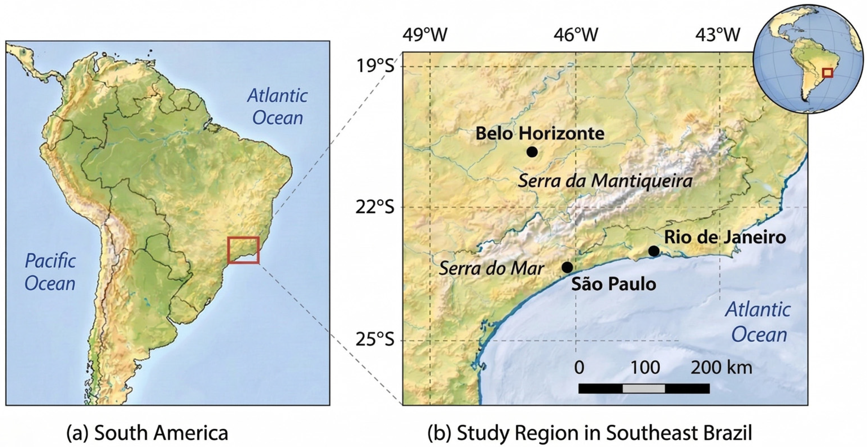
The Study Region is defined as a three-dimensional atmospheric volume bounded by longitudes 43° W to 49° W and latitudes 19° S to 25° S, with a vertical range extending from 500 hPa (approximately FL180) to 100 hPa (approximately FL500), where FL (Flight Level) refers to altitude in hundreds of feet (e.g., FL200 = 20,000 feet). This region encompasses the high-traffic air corridor between Rio de Janeiro and São Paulo, operationally known as the ‘Tubulão’ corridor (Rio–São Paulo air route), and extends to cover additional strategic routes connecting São Paulo, Rio de Janeiro, and Belo Horizonte—the three most important metropolitan centers in Southeast Brazil.

This corridor is recognized as the busiest and most operationally critical airspace in the country, concentrating a significant portion of commercial aviation activity. It also represents one of the regions with the highest incidence of reported turbulence events, particularly those associated with clear-air turbulence (CAT), due to the frequent interaction of jet streams, gravity waves, and wind shear in the upper troposphere over this area.

Figure 1 illustrates the defined Study Region (highlighted in blue). Within this area, a total of 20,338 turbulence occurrences were identified prior to methodological filtering, considering all reported VRTG events and turbulence intensity classes recorded by Airbus A320 aircraft operated by LATAM Airlines between 1 January 2018 and 31 December 2021. These events represent approximately 25% of the 82,951 turbulence occurrences documented by LATAM flights across South America during the same period, highlighting the disproportionately high concentration of turbulence within this specific airspace.

A detailed analysis of the CAT-related events further reveals a clear co-location between traffic density and reported turbulence incidence, confirming this region as a high-risk area for flight safety and a priority for turbulence forecasting efforts. These findings provide a strong justification for selecting this area as the focus of our study and support the broader goal of developing regionally adapted forecasting models capable of improving situational awareness and decision-making in complex and congested airspaces.

2.2. Analysis of Representative Severe CAT Events

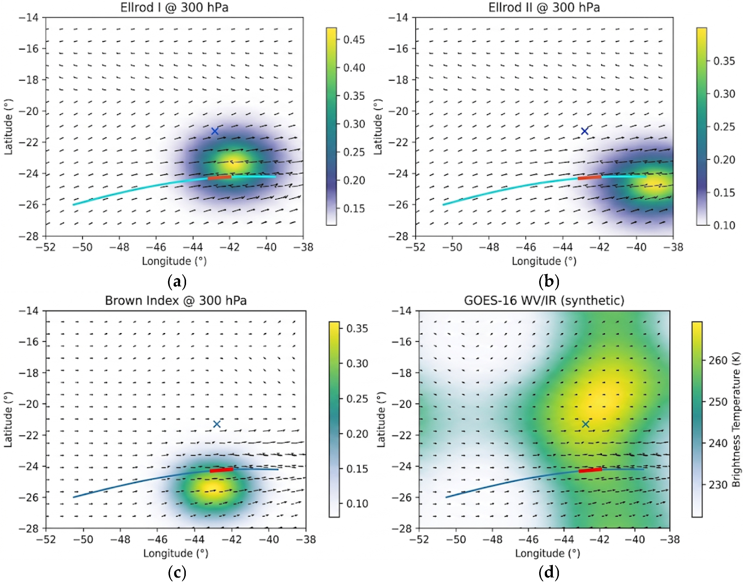
To illustrate known limitations of traditional turbulence diagnostics, we analyzed a confirmed severe CAT event recorded by a LATAM A320 aircraft over Southeast Brazil at cruise level (≥FL180). In this case, widely used operational indices, such as the Ellrod-1 (ELL1) and Ellrod-2 (ELL2) indices and the Brown index, indicated conditions favorable to turbulence in the analyzed region, although the maxima of these indices did not coincide exactly with the segment of the flight track where turbulence was reported.

This behavior is consistent with the spatial nature of CAT. In environments associated with subtropical jet streaks, gravity waves, or regions of intense wind shear, atmospheric instability may evolve and break at some distance from the forcing region, causing turbulence to manifest displaced from the maxima of the dynamical diagnostics [9]. Thus, although these indices are useful for identifying environments favorable to turbulence occurrence, the exact location where CAT manifests along the flight trajectory may present a small displacement relative to the dynamical structures identified.

Figure 2 presents the diagnostic fields at 300 hPa near the event time (±30 min). Panels (a–c) show the Ellrod 1, Ellrod 2, and Brown indices, while panel (d) shows the GOES-16 water-vapor/infrared brightness temperature, providing synoptic context for the upper-level flow. The maxima of the indices occur in the vicinity of the region where turbulence was reported by the aircraft, although they do not coincide exactly with the report location. This pattern illustrates a recurrent characteristic in CAT forecasting: classical diagnostics tend to indicate environments favorable to turbulence, while the observed event may occur slightly displaced from the maxima of these indices.

Values of the Ellrod and Brown indices may vary depending on the spatial resolution of the data, the numerical schemes used to compute gradients, and any smoothing applied to the atmospheric fields. These factors directly influence the magnitude of the estimated deformation and vertical wind shear. Therefore, the interpretation of these indices should be performed in a relative sense within the analyzed domain, with higher values (≈0.3–0.5) indicating greater turbulence potential, while lower values, close to zero, correspond to weak or non-turbulent conditions.

2.3. Data

The data utilized in this study originates from six distinct and reliable sources, each providing critical insights for identifying, classifying, and predicting turbulence events. Together, these datasets establish a robust framework for analyzing CAT within the Study Region.

Table 1. Summary of datasets used in this study, including source, temporal resolution, and role in CAT analysis.

Data	Frequency	Period	Description	Data Source/Reference
GFS	3 h	Two forecast times closest to the VRTG events	Global grid forecast at 0.25° resolution	NOAA—National Oceanic and Atmospheric Administration/ NCAR Research Data Archive, Boulder, CO, USA (RDA) (https://rda.ucar.edu/datasets/ds084.1/ (accessed on 5 March 2024))
METAR	1 h	1 January 2018–31 December 2021	Real-time weather observations critical for diagnosing CAT and no-CAT events	REDEMET—Brazilian Aeronautical Meteorological Network (https://www.redemet.aer.mil.br (accessed on 12 February 2024))
VRTG	Variable	1 January 2018–31 December 2021	Maximum vertical acceleration recorded over 60 min	LATAM Airlines operational flight data archive, Santiago, Chile (provided under research agreement, accessed on 8 January 2024)
TEMP	12 h	Selected days	Meteorological profile for São Paulo and Rio de Janeiro at 12Z/00Z	REDEMET—Brazilian Aeronautical Meteorological Network, Rio de Janeiro, Brazil (https://www.redemet.aer.mil.br (accessed on 21 February 2024))
GOES	15 min	Selected days	Infrared images (channels 4, 8, 13) for convective and high-level features.	CPTEC/INPE Satellite Data Archive, São José dos Campos, Brazil (http://satelite.cptec.inpe.br (accessed on 28 February 2024))
Synoptic Chart	6 h	Selected days	Surface-level conditions for analyzing large-scale patterns	CPTEC/INPE Operational Meteorological Charts

summarizes the datasets used, while their specific roles and applications are detailed below.

The Global Forecast System (GFS) data, acquired from the Research Data Archive at the National Center for Atmospheric Research, serves as the primary source of atmospheric model forecasts. These data offer global coverage with a grid resolution of 0.25° by 0.25° and are updated every three hours. To ensure alignment with turbulence events, the two forecast times closest to the occurrence of each event were selected for analysis.

Based on established physical understanding, specific atmospheric quantities, as detailed in Table 1, are correlated with CAT. The three-dimensional GFS variables analyzed include wind components u (zonal) and v (meridional), vertical velocity (w), and potential temperature (θ). Derived quantities such as vertical wind shear (VWS) between the pressure level of interest and the two adjacent levels, turbulent kinetic energy (TKE), and turbulence indices including the Richardson number [16], the Ellrod indices [9], and the Brown Index [17] were calculated to enhance the dataset. The total number of attributes—representing the value of each variable for every grid point within the defined three-dimensional rectangular volume (described in Section 2)—amounts to 67,500. This comprehensive dataset incorporates 12 three-dimensional variables, spanning 25 grid points in latitude, 25 grid points in longitude, and 9 vertical levels. Given the extensive nature of this dataset, a dimensionality reduction process was employed to isolate and prioritize the most relevant attributes for analysis.

Using the methodology outlined in the Section 2, the most significant attributes (or predictor features) were selected from these variables. These attributes, combined with labels for CAT and non-CAT events, were used to construct the training and testing datasets for the machine learning algorithms applied in this study. This selection process ensured that the machine learning models were informed by the most critical features, thereby optimizing their predictive accuracy.

The Vertical Acceleration of Gravity (VRTG) data, provided by LATAM Airlines, served as the core dataset for identifying and classifying turbulence events in this study. To ensure consistency and standardization across all measurements, only data recorded by a single aircraft model—the Airbus A320—were used. Covering the period from 1 January 2018 to 31 December 2021, this dataset includes the maximum VRTG recorded over the last 60 min at hourly intervals. VRTG measures deviations from the standard gravitational force (1 g) experienced during turbulence. The turbulence severity is classified into three categories: Class 1 (light), Class 2 (moderate), and Class 3 (severe), as presented in

Table 2. VRTG based turbulence classification.

Category	Negative g	Positive g
Non-turbulent conditions	0.6 < g < 1.4	0.6 < g < 1.4
Class 1 (Light)	0.4 < g ≤ 0.6	1.4 ≤ g < 1.6
Class 2 (Moderate)	0.2 < g ≤ 0.4	1.6 ≤ g < 1.8
Class 3 (Severe)	g ≤ 0.2	g ≥ 1.8

. These data were collected from LATAM’s fleet of A320 aircraft during routine flights, with measurements taken within a monitoring window starting 10 s after takeoff and ending 4 s before landing. It is important to note that the absence of VRTG data on a given day does not imply an absence of turbulence; it may simply reflect the absence of aircraft recording the phenomenon.

The turbulence intensity thresholds adopted by LATAM are based on operational experience and consider both upward and downward deviations from 1 g. The thresholds are asymmetric, reflecting the fact that upward (positive) and downward (negative) accelerations affect passenger perception and aircraft structural loads differently.

The TEMP (atmospheric soundings) data were obtained from the Brazilian aeronautical meteorological network operated by the Department of Airspace Control (DECEA). TEMP data provide meteorological profiles of temperature, relative humidity, and wind at standard pressure levels. TEMP soundings were used as contextual vertical profiles at synoptic times (00Z/12Z) to characterize the background stability and shear environment near the event day, acknowledging their limited temporal resolution.

METAR (Meteorological Aerodrome Reports) data, sourced from the Brazilian Aeronautical Meteorological Network (REDEMET) operational database, provide real-time weather observations critical for diagnosing turbulence conditions. METAR includes parameters such as wind speed, direction, visibility, cloud cover, and pressure. Reports from major airports in the Study Region, including São Paulo (Congonhas and Guarulhos), Rio de Janeiro (Santos Dumont and Galeão), and Belo Horizonte (Confins), were analyzed to differentiate CAT from turbulence caused by other weather phenomena. These localized observations, updated hourly, complement broader datasets and enhance event classification accuracy.

The GOES-16 satellite imagery, retrieved from the CPTEC/INPE operational satellite archive, offered high-resolution observations of atmospheric features relevant to turbulence. Thermal infrared imagery centered at 10.3 µm (channel 13) was the primary dataset used for detecting convective cells. Additionally, channel 8 (6.2 µm) and channel 4 (1.37 µm) were analyzed to identify cirrus clouds, gravity waves, and jet streams. These satellite images, collected at 15 min intervals, provided critical insights into atmospheric conditions conducive to CAT formation.

The synoptic charts, also obtained from REDEMET, present a detailed overview of surface-level atmospheric conditions, including pressure systems, weather fronts, wind patterns, and temperature distributions. Updated every six hours, these charts were vital for diagnosing large-scale meteorological patterns influencing turbulence events. Combined with TEMP and GOES-16 data, synoptic charts provided a robust framework for understanding the mechanisms driving turbulence.

In summary, the VRTG data served as the foundational dataset for identifying turbulence events, while the GFS data were used to extract predictor features for machine learning models. METAR, TEMP, GOES-16, and synoptic chart data provided additional context and support for identifying predictors, assisting in distinguishing CAT events from other types of severe turbulence initially selected based on VRTG.

By combining aircraft-recorded VRTG data, satellite imagery, synoptic analyses, and model outputs, this study establishes an efficient framework for analyzing and predicting CAT. This multidisciplinary approach enhances the understanding of factors driving CAT and contributes to developing machine learning models aimed at improving aviation safety. The specific roles of the datasets are summarized in Table 1, and Table 2 details the thresholds used for classifying turbulence severity based on VRTG.

The full mathematical formulation of the predictor variables derived from GFS fields is summarized in

Table 3. Selected Predictors from GFS data at grids points in the study area.

Input (Predictor)	Representation
$\mathrm{Zonal} \mathrm{wind} \mathrm{speed} \mathrm{at} \mathrm{level} zi$(kt)	$u \left(zi\right)$
$\mathrm{Meridional} \mathrm{wind} \mathrm{speed} \mathrm{at} \mathrm{level} zi$(kt)	$v \left(zi\right)$
$\mathrm{Vertical} \mathrm{wind} \mathrm{speed} \mathrm{at} \mathrm{level} zi$(kt)	$w \left(zi\right)$
$\mathrm{Horizontal} \mathrm{wind} \mathrm{speed} \mathrm{at} \mathrm{level} zi$(kt)	$ws \left(zi\right)=\sqrt{{\left[u \left(zi\right)\right]}^2+{\left[v \left(zi\right)\right]}^2}$
$\mathrm{Difference} \mathrm{in} \mathrm{horizontal} \mathrm{wind} \mathrm{speed} \mathrm{magnitude} \mathrm{between} \mathrm{levels} zi$$\mathrm{and} zj$(kt)	$∆ws \left(zi\right)=\sqrt{{\left[u \left(zi\right)\right]}^2+{\left[v \left(zi\right)\right]}^2}-\sqrt{{\left[u \left(zj\right)\right]}^2+{\left[v \left(zj\right)\right]}^2}$
$\mathrm{Vertical} \mathrm{wind} \mathrm{shear} \mathrm{between} \mathrm{levels} zi$ $\mathrm{and} zj$(s−1)	$vws \left(zi\right)=\sqrt{{\left[u \left(zi\right)-u \left(zj\right)\right]}^2+{\left[v \left(zi\right)-v \left(zj\right)\right]}^2}$
Potential temperature (K)	$\theta =T{\left({\displaystyle \frac{P}{P_0}}\right)}^{R_d/C_p}$
Turbulence kinetic energy (m2 s−2)	$TKE\left(zi\right)=0.5\left[{\left[u \left(zi\right)\right]}^2+{\left[v \left(zi\right)\right]}^2+{\left[w \left(zi\right)\right]}^2\right]$
Gradient Richardson number	$Ri={\displaystyle \frac{N^2}{{\left(\frac{dU}{dz}\right)}^2}}$
Brown index (s−1)	$\Phi m=\sqrt{0.3\times {\left({\displaystyle \frac{\partial v}{\partial x}}-{\displaystyle \frac{\partial u}{\partial y}}+f\right)}^2+{\left({\displaystyle \frac{\partial v}{\partial x}}+{\displaystyle \frac{\partial u}{\partial y}}\right)}^2+{\left({\displaystyle \frac{\partial u}{\partial x}}-{\displaystyle \frac{\partial v}{\partial y}}\right)}^2 }$
Ellrod index 1 (s−1)	$El1=DEF\times VWS$
Ellrod index 2 (s−1)	$El2=VWS\times \left(DEF+CVG\right)$
Ellrod index 3 (s−1)	$El3=El1+DVT$

$u$, $v$, $w$ wind components; $ws$ horizontal wind speed; $zi$, $zj$ levels; $T$ temperature; $P_0$ = 1000 hPa; $R_d/C_p$ thermodynamic constants; $N^2$ Brunt–Väisälä frequency; $f$ Coriolis parameter; $DEF$ deformation; $CVG$ convergence; $VWS$ vertical wind shear; $DVT$ divergence tendency.

, including wind components, thermodynamic quantities, and turbulence diagnostics used as candidate features in the supervised learning framework.

VRTG data were used to identify turbulence events within the study region (Figure 1). Events were classified according to operational intensity thresholds (Class 1–3), and severe CAT (Class 3) cases were retained as the positive class. The distinction between severe CAT and non-CAT conditions was confirmed through multi-source screening, as described in Section 2.2.

Although Eddy Dissipation Rate (EDR) is widely recognized as the standard aircraft-independent turbulence metric recommended for aviation applications, EDR observations were not available for the dataset used in this study. In many turbulence investigations, aircraft response variables such as vertical acceleration or derived g-load metrics are used as practical proxies for turbulence intensity. These measurements directly reflect the dynamical response of the aircraft to atmospheric turbulent motions and have therefore been widely adopted in observational turbulence datasets. When restricted to cruise-level flight segments, where pilot-induced maneuvers are minimal, vertical acceleration measurements provide a robust indicator of severe turbulence events [5].

2.4. Feature Selection

The selection of predictor attributes (inputs) is a critical step in the development of machine-learning-based predictive models, as it directly affects model accuracy, computational efficiency, and generalization capability. In this study, the objective is to discriminate between time slots with and without the occurrence of severe CAT, as defined by aircraft-reported vertical acceleration (VRTG) and independent observational screening.

The predictor attributes were derived from the GFS025 model and consist of twelve atmospheric predictors: the zonal wind component (u), meridional wind component (v), vertical wind velocity (w), potential temperature (θ), horizontal wind speed magnitude (VEL), vertical wind shear (VWS), turbulent kinetic energy (TKE), gradient Richardson number (Ri), the Brown turbulence index (Brown), and the Ellrod turbulence indices (Ell1, Ell2, and Ell3). These predictors are distributed over a spatial grid of 25 latitude points by 25 longitude points and across nine vertical levels. This configuration results in a total of 67,500 potential predictors per sample, characterizing a high-dimensional feature space. Given this dimensionality, attribute selection is essential to reduce computational cost, eliminate redundant or weakly informative predictors, and enhance model performance. This process, commonly referred to as dimensionality reduction, aims to identify relevant patterns and extract meaningful information from large datasets while preserving the physical representativeness of the atmospheric fields [18,19]. Simplified representations have been shown to improve learning efficiency and robustness in complex classification problems [20].

In this study, statistical hypothesis testing was adopted as the primary method for supervised attribute selection. Predictor relevance was evaluated directly with respect to the target classification (CAT versus non-CAT), consistent with the supervised learning framework employed. The statistical significance of each candidate attribute was assessed using Student′s t-statistic to compare the mean values of the predictor distributions between severe CAT events (Class 3) and non-CAT cases. The significance level was estimated using a permutation-based approach, in which class labels were randomly permuted 10,000 times to obtain an empirical distribution of the $t$ -statistic. This procedure was implemented using the BRB-ArrayTools framework, National Cancer Institute (NCI), Bethesda, MD, USA [21,22,23].

The t-statistic is defined as:

$$t={\displaystyle \frac{X1-X2}{\sqrt{\left(\frac{S_1^2}{n_1}\right)+\left(\frac{S_2^2}{n_2}\right)}}},$$

(1)

where $X1$ and $X2$ are the means of samples 1 and 2, $S_1$ and $S_2$ are the variances of samples 1 and 2, and $n_1$ and $n_2$ are the sample sizes. The p-value (p) was estimated using a permutation-based procedure. The class labels were randomly permuted 10,000 times (Np) to generate an empirical distribution of the $t$ -statistic. The p-value corresponds to the proportion of permutations in which the absolute value of the permuted $t$ -statistic equals or exceeds the observed value. Six significance thresholds were evaluated (α = 0.01, 0.005, 0.001, 10⁻⁴, 5 × 10⁻⁵, and 10⁻⁵):

$$p={\displaystyle \frac{number of permutations with \left|t\right|\ge \left|t_{observed}\right|}{1+N_p}},$$

(2)

The null hypothesis (H₀) assumes no statistically significant difference between the predictor distributions for severe CAT and non-CAT events. A p-value lower than the selected significance level provides sufficient evidence to reject H₀, indicating that the predictor contributes to discriminating between the two classes.

To operationalize the attribute selection procedure, the BRB-Array Tools software v4.6 [21,22,23], originally developed by the U.S. National Cancer Institute for large-scale genomic analyses, was adapted for meteorological applications. In this framework, originally developed for genomic data and adapted here to meteorological predictors, and disease outcomes were replaced by CAT occurrence. This adaptation enables efficient processing of high-dimensional atmospheric datasets while applying statistical controls.

Given the large number of simultaneous hypothesis tests, the FDR method was applied to control the proportion of false positives among statistically significant results [24]. The FDR is defined as FDR = V/R, where V represents the number of false discoveries of the null hypothesis (H₀) and R is the total discoveries (rejections). By limiting the expected proportion of false discoveries, FDR control ensures a balanced trade-off between statistical rigor and sensitivity in large-scale feature selection problems.

Another relevant aspect concerns the potential presence of spatial autocorrelation among the atmospheric predictors used in this study. Outputs from numerical weather prediction models inherently exhibit spatial dependence, as neighboring grid points tend to be statistically related due to the continuous and dynamically coherent nature of atmospheric fields. Consequently, some predictors derived from these fields may share correlated spatial structures. In this study, the attribute selection procedure was applied with the objective of reducing redundancy and identifying a compact set of physically interpretable predictors. Nevertheless, future investigations may explore feature selection strategies that explicitly account for spatial dependence in order to further assess the impact of spatial autocorrelation on model performance.

In this study, the FDR procedure is applied exclusively within the statistical attribute selection stage, with the sole objective of identifying predictors that exhibit robust and statistically significant differences between CAT and non-CAT samples. Importantly, the FDR does not evaluate classification performance and does not influence the training or assessment of the supervised machine learning models, which are addressed in a subsequent stage of the analysis. This procedure ensures that the retained predictors represent statistically robust atmospheric signals associated with severe CAT occurrence while minimizing the inclusion of spurious correlations in the final feature set.

To prevent information leakage, feature selection was performed independently within each training fold during the 5-fold cross-validation procedure. For each fold, statistical hypothesis testing and FDR control were applied exclusively to the training subset, and the selected predictors were subsequently used to train and validate the model within that fold.

2.5. Machine Learning Models

The dataset used for training and testing the supervised learning models consists of hourly records of the selected predictor attributes concatenated with a binary target variable (“yes” or “no”). Severe CAT cases (TARGET = yes) are defined exclusively based on aircraft-reported vertical acceleration, with Class 3 VRTG events representing the positive class. For each severe event, the corresponding GFS predictor fields are extracted from the two time slots closest to the occurrence. Non-CAT samples (TARGET = no) correspond to cruise-level time slots in which no turbulence exceeding the defined operational threshold was recorded by the instrumented aircraft (VRTG = 0). This classification reflects the absence of detected turbulence along the sampled flight trajectory rather than a definitive absence of atmospheric instability and should therefore be interpreted within the inherent spatial and observational limitations of aircraft-based turbulence measurements. The balanced case–control design was adopted exclusively for discriminative modeling and does not represent operational CAT prevalence. This sampling strategy was adopted to mitigate the strong class imbalance inherent to severe CAT occurrence datasets, reduce bias toward the dominant non-CAT class, and provide a controlled basis for comparing classifier discrimination under rare-event conditions.

All severe CAT cases (N = 85; Class 3 VRTG) were retained for the supervised modeling stage. To construct a balanced case–control dataset, an equal number of non-CAT samples (N = 85) was randomly selected from the negative class, resulting in 170 labeled instances. Stratified 5-fold cross-validation was adopted, maintaining class balance within each fold (≈17 severe cases per test fold). Although the number of severe events is constrained by the observational record, the stratified cross-validation framework ensures that each severe case is evaluated in out-of-sample conditions exactly once, reducing sensitivity to single-split variability and limiting overfitting risk.

The training process included hyperparameter optimization using a grid search approach. Different hyperparameter configurations were systematically evaluated for each algorithm to identify the optimal settings that maximize prediction accuracy and model robustness. This approach ensures that the machine learning models are fine-tuned and capable of effectively distinguishing between severe CAT events (VRTG class 3) and non-CAT conditions.

2.6. Evaluation Metrics

The performance of the developed models is assessed using appropriate metrics. Given the limitations of VRTG data, which do not provide a systematic or comprehensive sampling of the airspace, traditional scalar statistics such as False Alarm Rate (FAR) and Prediction Bias (BIAS) cannot be reliably calculated [25]. These metrics require consistent and representative sampling, which the restricted and non-uniform nature of VRTG data does not provide. Then, in this study, turbulence prediction is treated as a binary classification problem: the model predicts whether turbulence occurs (positive event) or not (negative event). This approach results in four possible outcomes: True Positive (TP): Correct prediction of turbulence occurrence, False Positive (FP): Incorrect prediction of turbulence occurrence, False Negative (FN): Failure to predict turbulence, and True Negative (TN): Correct prediction of no turbulence.

The model performance is evaluated using the Receiver Operating Characteristic (ROC) curve and the Area Under the ROC Curve (AUC). These metrics are widely recognized in turbulence prediction [11,26,27,28,29,30].

The ROC curve is a graphical representation of the performance of a binary classifier as the discrimination threshold varies. It plots two main metrics: True Positive Rate (PODy), representing the proportion of correctly predicted positive events, and False Positive Rate (1$-$PODn), representing the proportion of incorrectly predicted negative events given by Equations (3) and (4). For example,

$$PODy={\displaystyle \frac{TP}{TP+FN}},$$

(3)

$$PODn={\displaystyle \frac{TN}{TN+FP}},$$

(4)

where TP: True Positives (correctly predicted turbulence events), FN: False Negatives (missed turbulence events), TN: True Negatives (correctly predicted no-turbulence events), and FP: False Positives (incorrectly predicted turbulence events).

The Area Under the ROC Curve (AUC) is a single scalar value that quantifies the overall performance of a binary classifier. It reflects the model’s ability to distinguish between positive and negative classes. An AUC value close to 1 indicates a near-perfect classifier, and an AUC value of 0.5 signifies a random classification, equivalent to guessing [26,27].

The AUC metric provides an objective evaluation of model performance, with higher values indicating improved discrimination between severe CAT and non-CAT events. To address the strong class imbalance inherent to CAT occurrence datasets, a balanced case–control design was adopted for discriminative modeling, ensuring equal representation of severe CAT and non-CAT samples during model training. Model performance was subsequently assessed using stratified 5-fold cross-validation, preserving class proportions within each fold to maintain statistical consistency and reduce sampling variability. Because this balanced design does not reproduce real-world CAT prevalence, the resulting ROC/AUC values should be interpreted primarily as measures of relative discriminative performance within the adopted experimental framework rather than as direct indicators of operational event frequency or climatological forecast skill. Given the narrow performance margins among the top-tier models and the rare-event nature of the dataset, the evaluation focused on the consistency of discriminative capability under rigorous validation, rather than seeking strict statistical superiority among individual classifiers. The use of pairwise significance tests on a sample size of N = 85 could result in low statistical power; therefore, it was replaced by a detailed analysis of inter-fold variability (AUC ± SD), ensuring the transparency and reproducibility of the regional framework.

3. Results

This section provides a detailed discussion of the findings, following the sequence of steps outlined in the methodology. It includes an analysis of VRTG data, the process of defining a balanced case–control sample of CAT and non-CAT events, the selection of predictor attributes, and the subsequent training of machine learning algorithms. Each step is critically evaluated to underscore its contribution to understanding the dynamics of clear-air turbulence and enhancing prediction accuracy.

3.1. VRTG Analysis

The procedure described in Section 2 was applied to classify CAT and non-CAT events using aircraft-reported vertical acceleration (VRTG) complemented by multi-source observational screening. After applying cruise-level and quality-control filters to the initial 20,338 events identified within the study region, 8550 events were retained for detailed VRTG analysis. This filtered dataset focuses on cruise-level conditions and forms the basis for the subsequent classification and modeling steps. Of these events, 92% were classified as light (Class 1), 7% as moderate (Class 2), and 1% as severe turbulence (Class 3).

With respect to the vertical distribution, 88% of the recorded events (7523 occurrences) were observed between flight levels FL180 and FL300, while the remaining 1027 events occurred above FL300. This concentration reflects the typical cruise-level range of commercial aviation and is consistent with the altitude band where jet-related shear and deformation processes are most active over the study region.

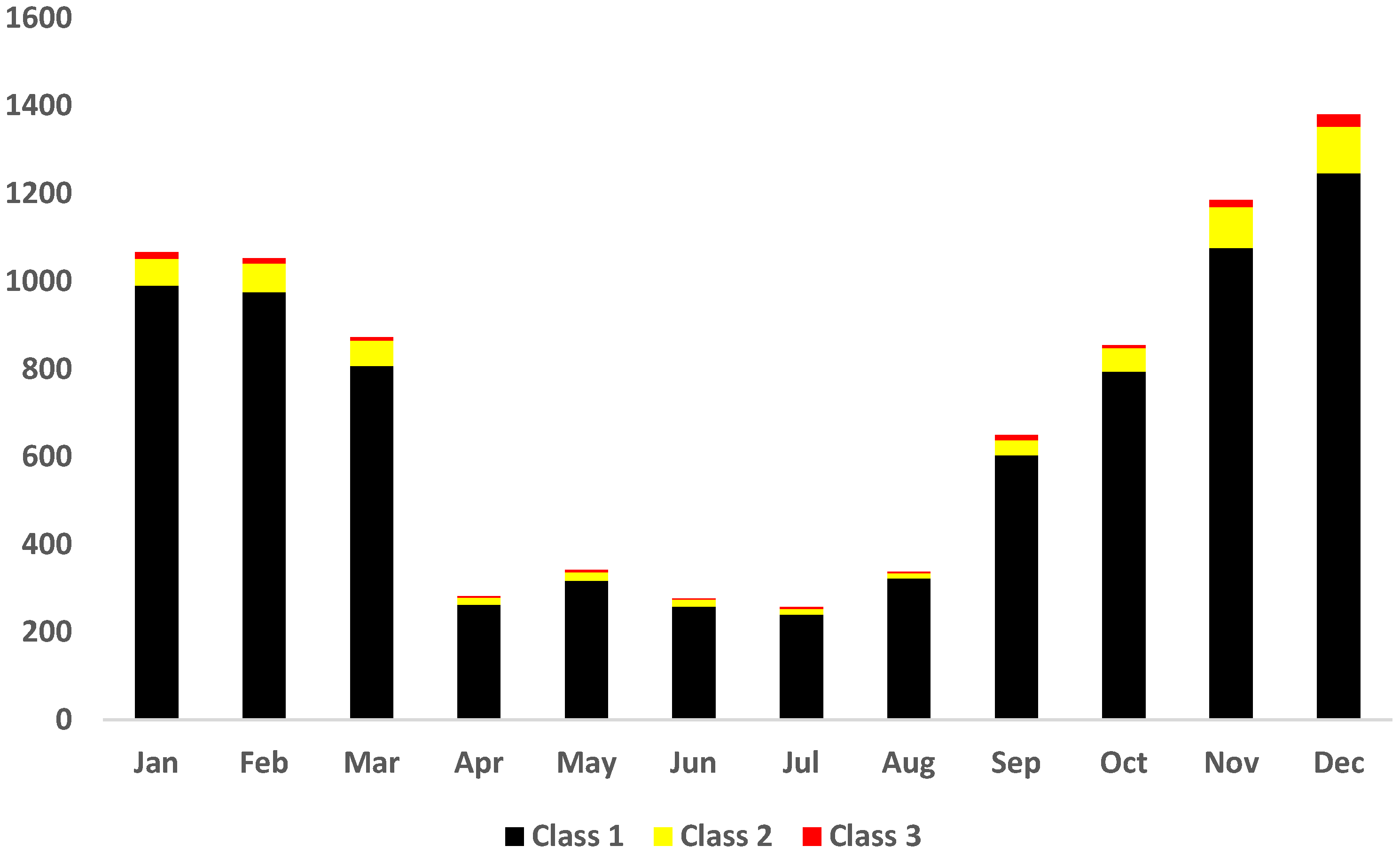
The monthly variability of VRTG occurrences, shown in Figure 3, reveals a marked seasonal modulation, with increased turbulence records during late spring and summer (November to March). This behavior is consistent with enhanced convective activity and the associated generation of gravity waves, which are known to modulate upper-level flow and favor the occurrence of clear-air turbulence [10,28,29].

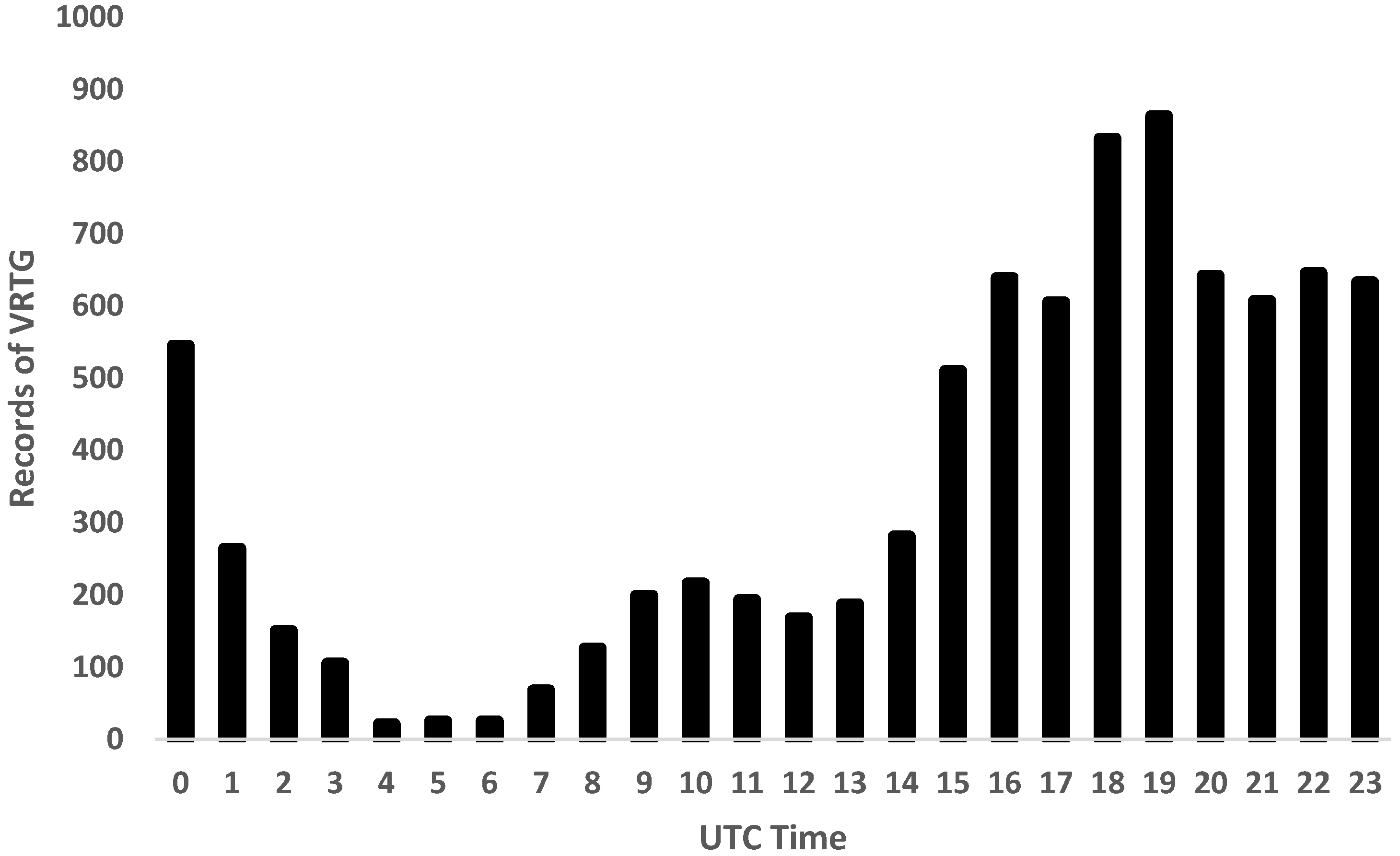
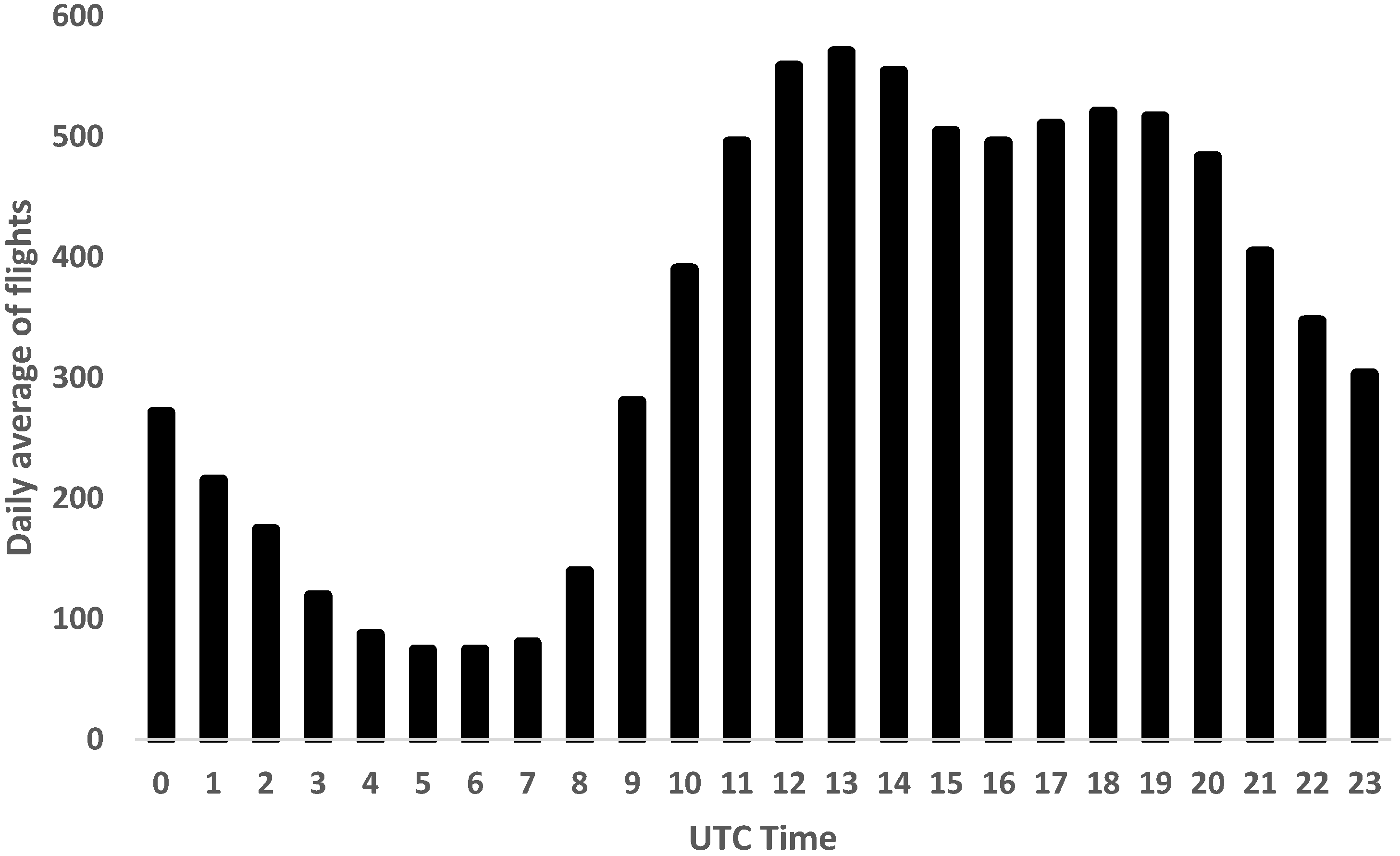
Figure 4 and Figure 5 present the hourly distribution of VRTG reports and flight operations, respectively, and are included to characterize the temporal availability of observational data within the analyzed period. These distributions are shown for descriptive purposes only and are not used to infer causal relationships between time of day and turbulence occurrence.

The interpretation of the hourly distribution of VRTG records (Figure 4) should be performed in conjunction with the distribution of flight operations (Figure 5). In general, a reduction in the number of VRTG records is observed during certain periods of the day, associated both with a decrease in air traffic volume and with greater atmospheric dynamical stability during those times.

3.2. Selection of Predictor Attributes

The selected predictor attributes were extracted from three-dimensional (3D) meteorological fields defined over a local grid composed of 25 × 25 horizontal points, 9 vertical levels, and 12 variables forecast by the GFS025 model. This configuration yields 67,500 candidate attributes for each event time slot (25 × 25 × 9 × 12 = 67,500). Considering that this feature extraction was repeated for all analyzed event time slots, the complete database comprised millions of candidate attribute values over the study period. Therefore, the dimensionality problem addressed in this study refers to a high-dimensional predictor space with 67,500 potential predictors per sample, rather than to a fixed set of 27.1 million independent predictors. Such dimensionality is clearly incompatible with empirical and theoretical constraints widely established in the statistical and machine learning literature, which indicate the need for a minimum ratio on the order of 10:1 to 20:1 between the number of independent samples (or events) and the number of predictor variables in order to ensure statistical stability, generalization capability, and robustness against overfitting [30,31,32]. Therefore, the adoption of a feature selection strategy was not merely a computational convenience but a methodological requirement. The dimensionality reduction process employed in this study was specifically designed to reconcile the available sample size with established best practices in supervised learning, while preserving physical interpretability of the atmospheric predictors.

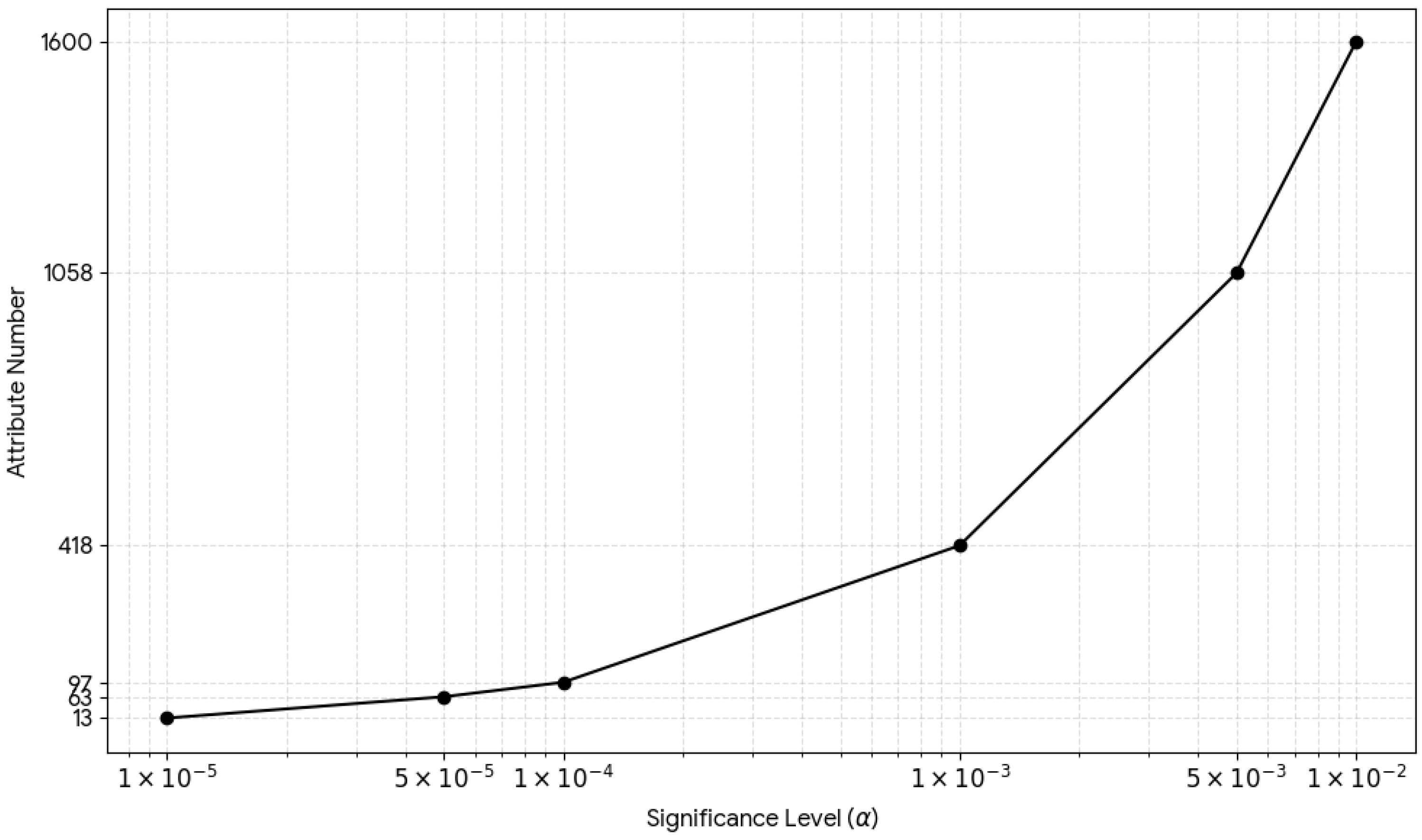
Figure 6 illustrates the progressive reduction in the number of retained attributes across different significance levels (α = 10⁻⁵, 5 × 10⁻⁵, 10⁻⁴, 0.001, 0.005, and 0.01), presented on a logarithmic scale. These thresholds correspond to 13, 48, 97, 418, 1058, and 1600 retained attributes, respectively. Lower p-values indicate stronger statistical separation between severe CAT events and non-CAT conditions, reflecting a higher discriminatory potential of the corresponding predictors within a supervised classification framework.

High dimensionality in the predictor space increases model complexity, leading to overfitting, longer training times, and reduced generalizability. To mitigate these effects, a conservative significance level of α = 10⁻⁵ was adopted, resulting in a compact subset of 13 statistically relevant predictors. This choice represents a balance between dimensionality reduction and physical representativeness, ensuring that the retained attributes capture the most robust differences between CAT and non-CAT samples without introducing unnecessary redundancy.

At this stage of the analysis, the objective is strictly limited to statistical relevance and dimensionality reduction. No classification rules, physical thresholds, or performance metrics are derived or evaluated here. The selected predictors constitute the input feature set for the supervised learning experiments described in the subsequent section.

3.2.1. Attribute Selection Results and Analysis

Dimensionality reduction was performed by selecting the most statistically significant attributes based on their p-values obtained from supervised hypothesis testing [21,22,23,24].

Table 4. Top 13 predictor attributes ranked by p-values and false discovery rate (FDR) at significance level of α = 10⁻⁵.

Order of Significance	p-Value	FDR	Attribute (Variable_Coordinates_Altitude)
1	6.00 × 10−8	0.003	ELL2_−45.5_−19.75_300
2	1.00 × 10−7	0.003	BROWN_−48.0_−19.25_300
3	7.00 × 10−7	0.0135	ELL2_−44.0_−20.75_300
4	9.00 × 10−7	0.0135	BROWN_−48.0_−19.0_300
5	1.20 × 10−6	0.0144	ELL2_−46.0_−19.5_300
6	2.00 × 10−6	0.02	BROWN_−47.75_−19.25_300
7	5.40 × 10−6	0.036	ELL2_−47.25_−21.5_250
8	6.00 × 10−6	0.036	w_−48.75_−21.75_350
9	6.60 × 10−6	0.036	ELL3_−46.25_−19.5_300
10	6.80 × 10−6	0.036	BROWN_−47.75_−19.0_300
11	7.10 × 10−6	0.036	BROWN_−47.75_−21.0_250
12	7.20 × 10−6	0.036	ELL2_−44.75_−20.25_300
13	9.90 × 10−6	0.0457	ELL2_−46.25_−19.25_300

summarizes the significance ranking of the 13 retained predictor attributes, ordered according to increasing p-values and their corresponding False Discovery Rate (FDR) values. These predictors were extracted from three-dimensional meteorological fields produced by the GFS model over the study region and evaluated directly with respect to the CAT versus non-CAT classification.

The selected attributes exhibit p-values ranging from 0.6 × 10⁻⁷ to 9.9 × 10⁻⁶, with all associated FDR values remaining below 0.05. This confirms that the likelihood of false positives among the retained predictors is low, supporting the statistical robustness and reliability of the dimensionality reduction process.

The most significant predictors include turbulence-related diagnostics widely recognized in the literature as indicators of dynamically unstable atmospheric conditions. Among them, the Ellrod indices (ELL2 and ELL3), and the Brown index, stand out as physically consistent contributors:

▪

ELL2 and ELL3 (Ellrod indices): diagnostic formulations that combine horizontal deformation and vertical wind shear, widely used to identify atmospheric environments favorable to clear-air turbulence [9].

▪

BROWN: combines vertical wind shear and horizontal deformation, two dynamical ingredients commonly associated with clear-air turbulence-favorable environments. The spatial and vertical distribution of the retained predictors is predominantly concentrated between flight levels FL250 and FL350 (approximately 25,000–35,000 ft), with horizontal coordinates mainly located within the core of the study region, bounded by longitudes −48.75° W to −43.0° W and latitudes −21.75° S to −19.0° S. This configuration is physically consistent with the altitude range of cruise-level operations and with the dynamical environment of the mid-to-upper troposphere, where jet-related shear, deformation, and wave activity are most pronounced.

3.2.2. Implications of Attribute Selection

The identification of these statistically significant predictors provides important insights into the atmospheric mechanisms associated with CAT occurrence. The dominance of variables related to wind shear, horizontal deformation, and vertical motion highlights the role of localized dynamical structures in triggering turbulence. These processes are consistent with jet-related shear zones and mesoscale perturbations commonly observed in clear-air turbulence environments. The low p-values confirm the statistical robustness of the selected attributes, supporting their suitability for subsequent use in supervised machine learning models.

In conclusion, the results validate the effectiveness of the p-value-based approach, combined with FDR control, for dimensionality reduction and attribute selection in high-dimensional atmospheric datasets. Under the most conservative setting (α = 10⁻⁵), only 13 attributes are retained (Figure 6), and Table 4 summarizes the corresponding top predictors ranked by p-values and FDR. Table 4 emphasizes the relevance of ELL2 and BROWN as physically meaningful predictors associated with CAT-favorable flow configurations. This refined attribute set preserves physical interpretability while reducing redundancy, providing a consistent basis for subsequent modeling efforts.

The final attribute set, combined with the target variable (“yes” for CAT events and “no” for non-CAT events), forms the input dataset for training and testing the supervised machine learning algorithms discussed in subsequent sections.

3.3. Training and Testing of Machine Learning Algorithms

To ensure reliable generalization and minimize the risk of overfitting, the machine learning (ML) workflow in this study was designed to balance model complexity and validation rigor. Nine algorithms were evaluated to assess predictive performance: Logistic Regression, Random Forest, Decision Tree, Gradient Boosting, AdaBoost, K-Nearest Neighbors (KNN), Support Vector Machine (SVM), Naive Bayes, and Multi-Layer Perceptron (MLP)—to classify turbulence events with varying degrees of severity.

A critical step to prevent overfitting was the application of 5-fold cross-validation during model training. In this strategy, the training dataset was partitioned into five equally sized folds, and for each combination of predictors (ranging from 1 to 13), the model was trained on four folds and validated on the remaining one. This process was repeated five times per configuration, ensuring that each data point was used for both training and validation. This technique reduces the risk of a model becoming too tailored to a specific training subset and promotes a more robust estimation of performance on unseen data.

To further reinforce generalization and prevent model overfitting, grid search hyperparameter tuning was conducted within each cross-validation cycle. For each algorithm, multiple combinations of hyperparameters were systematically tested, as detailed in

Table 5. Hyperparameter search space, number of combinations, and total training iterations using 5-fold cross-validation (k = 1–13) for each machine learning algorithm.

Algorithm	Hyperparameters	Hyperparameter Combinations	Training Iterations (5-Fold, k = 1 to k = 13)
Logistic Regression [30]	C: [0.01, 0.1, 1, 10, 100], solver: [‘liblinear’, ‘saga’], max_iter: 2000	10	50 × 13 = 650
Random Forest [27]	n_estimators: [50, 100, 200, 300], max_depth: [None, 10, 20, 30, 40]	20	100 × 13 = 1300
Decision Tree [33]	max_depth: [None, 10, 20, 30], min_samples_split: [2, 10, 20]	12	60 × 13 = 780
Gradient Boosting [34]	n_estimators: [50, 100, 200], learning_rate: [0.01, 0.1, 0.2]	9	45 × 13 = 585
AdaBoost [26]	n_estimators: [50, 100, 200], learning_rate: [0.01, 0.1, 1], algorithm: ‘SAMME’	9	45 × 13 = 585
K-Nearest Neighbors [35]	n_neighbors: [3, 5, 7], weights: [‘uniform’, ‘distance’]	6	30 × 13 = 390
Support Vector Machine [36]	C: [0.1, 1, 10], kernel: [‘linear’, ‘rbf’], probability: True	6	30 × 13 = 390
Naive Bayes [29]	None	1	5 × 13 = 65
Multi-Layer Perceptron [28]	hidden_layer_sizes: [(10,), (20,), (30,)], activation: [‘relu’, ‘logistic’], max_iter: 2000, solver: ‘adam’	6	30 × 13 = 390
Total		79	5635

. This ensured that models were not only fit to the data but also optimized with the best ML hyperparameters that generalized well across folds. For instance, Random Forest and Gradient Boosting models underwent extensive search over multiple depth and ensemble size parameters, while simpler models like Naive Bayes required minimal tuning.

Hyperparameter optimization and performance estimation were conducted exclusively within the 5-fold cross-validation framework. AUC values are reported as mean ± standard deviation across the five validation folds, providing an empirical estimate of performance variability under out-of-sample conditions. This procedure provides a robust estimate of generalization performance while reducing the risk of overfitting.

Model performance was primarily assessed using the Receiver Operating Characteristic (ROC) curve and the corresponding Area Under the Curve (AUC) metric. These tools offer a threshold-independent evaluation of a classifier’s ability to distinguish between severe CAT events (Class 3, TARGET = yes) and screened non-CAT samples (VRTG = 0, TARGET = no).

As summarized in Table 5, the total number of training iterations resulted from the combination of predictors, cross-validation folds, and hyperparameter grids.

Machine Learning Model Performance

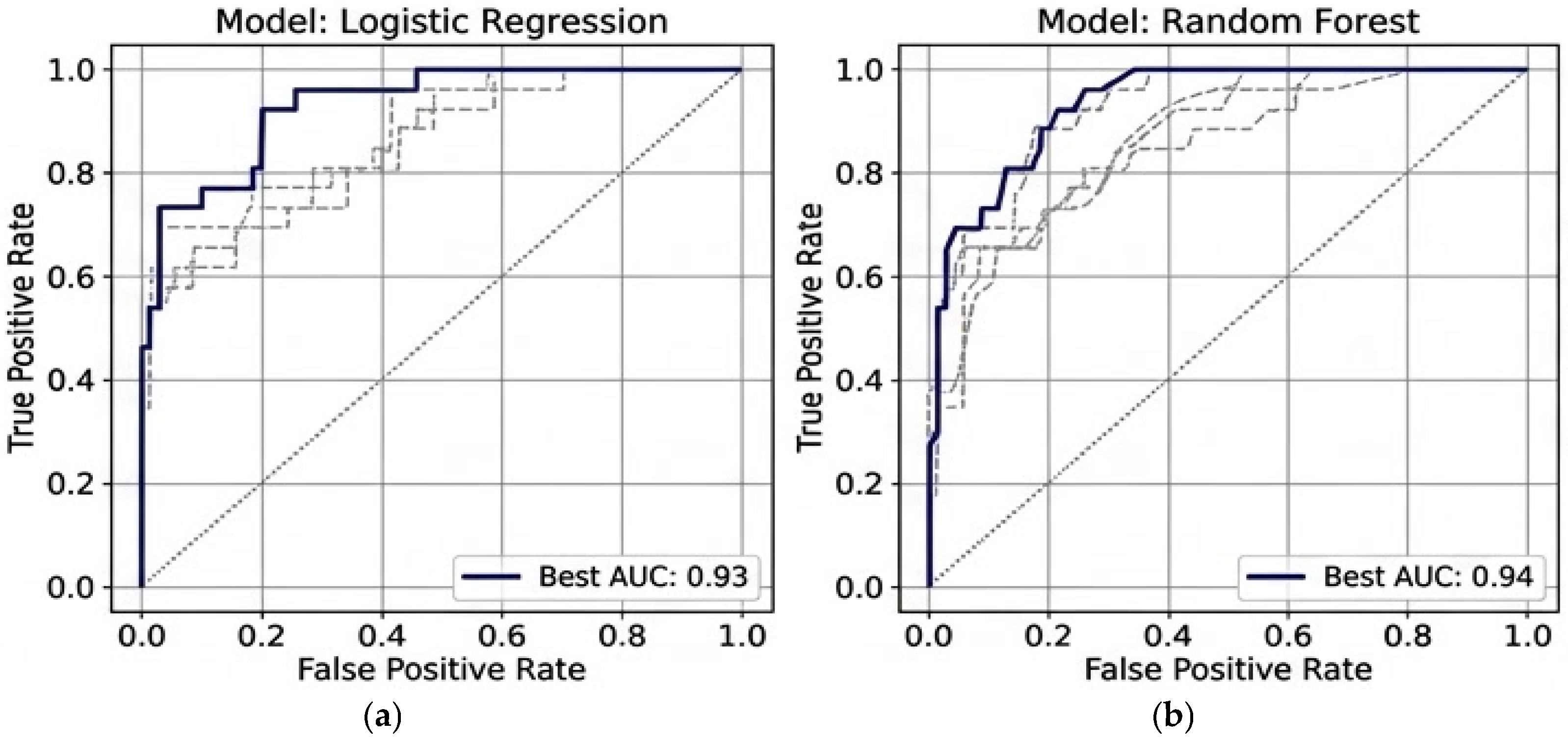
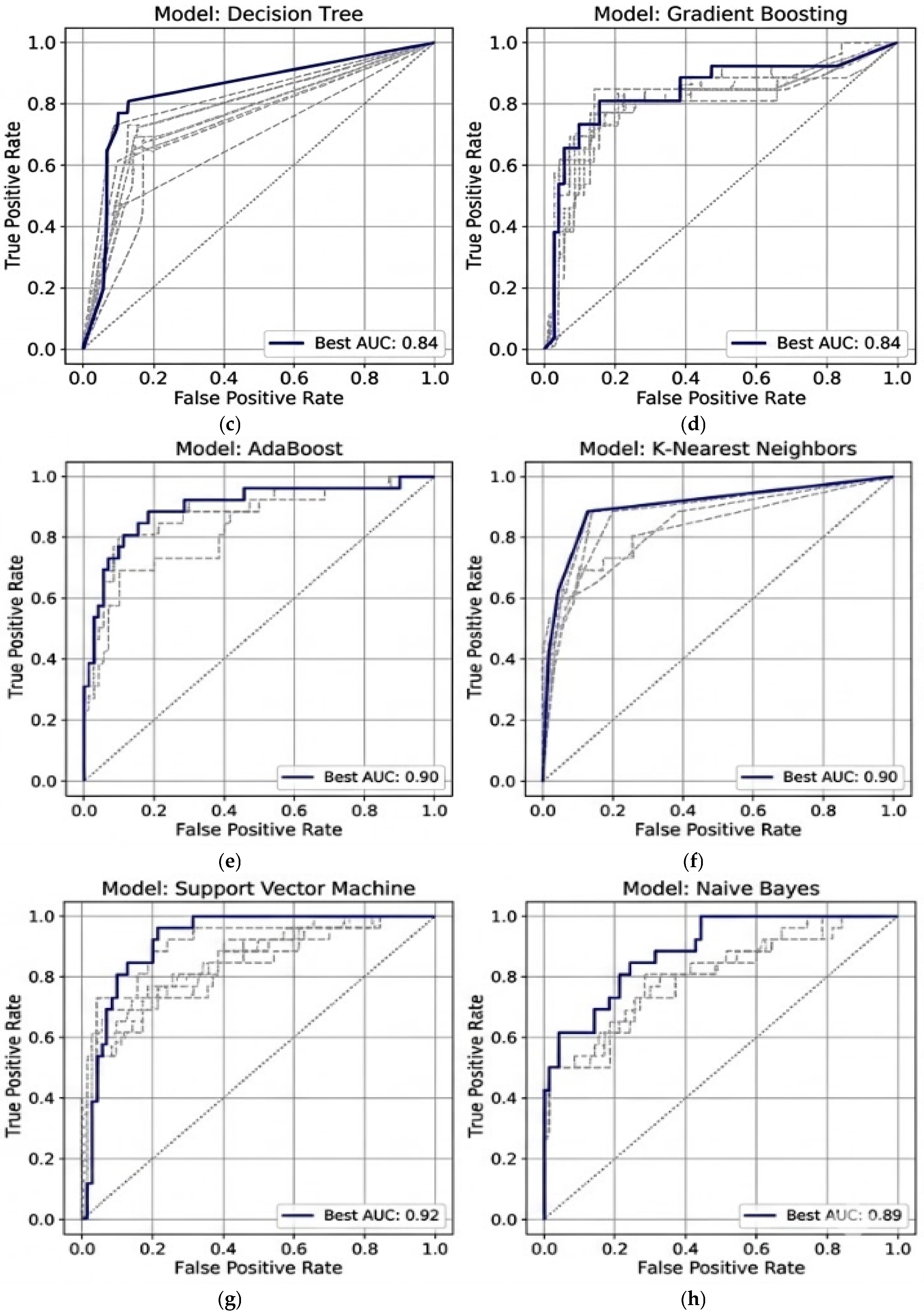
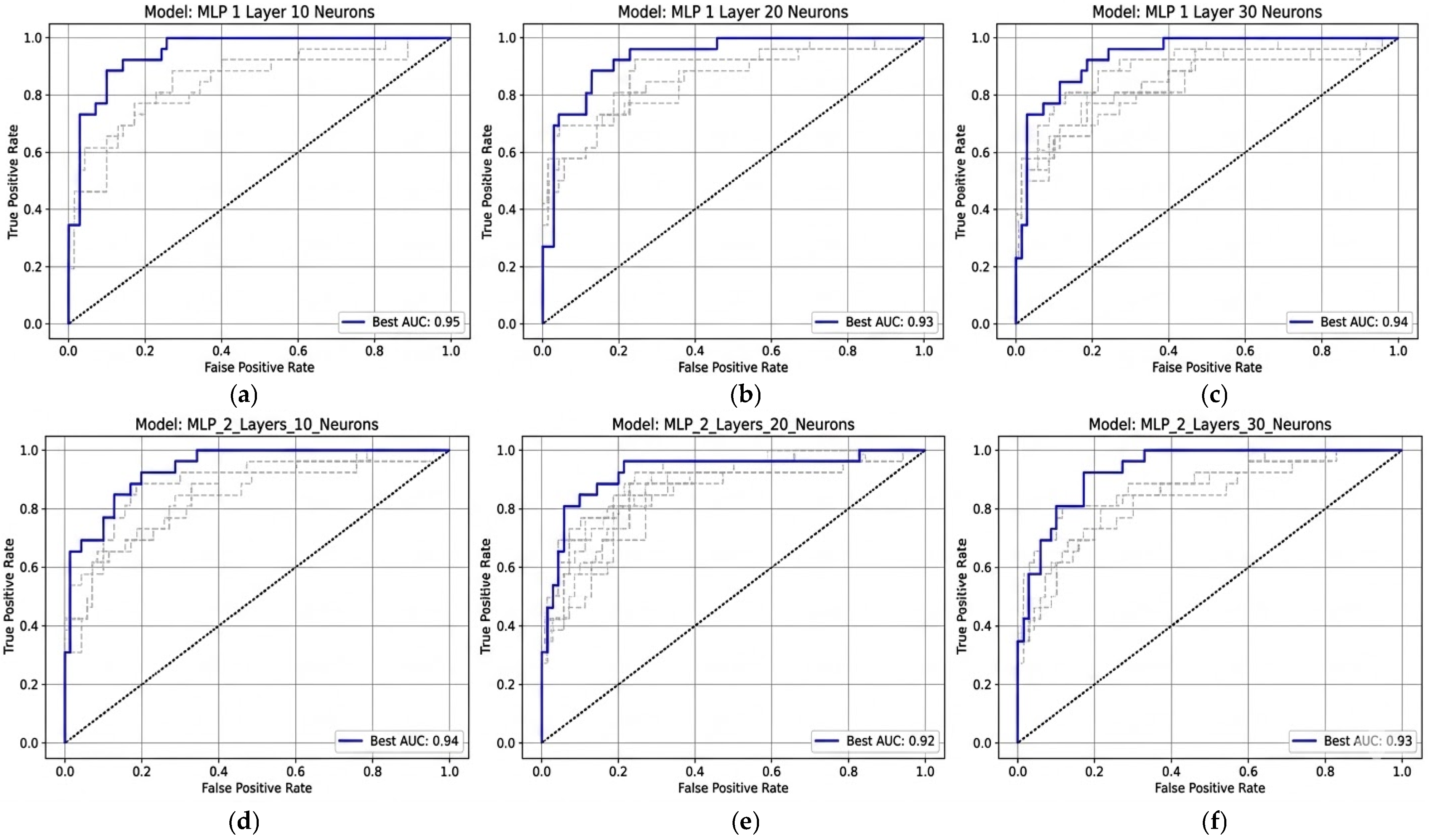
This section presents the performance analysis of machine learning models for predicting CAT events based on ROC curves and their corresponding AUC values. To enhance visual clarity, the remaining ROC curves from the 5-fold cross-validation are shown with thinner dashed gray lines, minimizing visual noise, while the curve with the highest AUC is highlighted more prominently. A diagonal reference line representing random model performance is included for comparison. The ROC curve with the highest AUC is highlighted using a solid blue line. Figure 7a–h presents the ROC curves for Logistic Regression, Random Forest, AdaBoost, K-Nearest Neighbors (KNN), Decision Tree, Support Vector Machine (SVM), Gradient Boosting, and Naive Bayes.

Standard deviations for lower-performing models remained within ±0.05 and did not alter the relative ranking among classifiers.

Figure 8a–f presents the ROC curves for the Multi-Layer Perceptron (MLP) models with one and two hidden layers and 10, 20, and 30 neurons, respectively.

The Multi-Layer Perceptron (MLP) with one hidden layer of 10 neurons achieved the highest numerical AUC (0.95 ± 0.03), indicating strong discriminative capability. However, several other algorithms also achieved comparable performance, including Random Forest (AUC = 0.94 ± 0.04) and Logistic Regression (AUC = 0.93 ± 0.04), suggesting that multiple model architectures are capable of capturing the relevant atmospheric patterns associated with severe CAT events. Simpler MLP architectures (one layer) consistently outperformed more complex configurations (two layers), indicating that additional layers or neurons do not necessarily improve performance. For instance, MLP with one layer and 10 neurons outperformed MLP with two layers and 20 neurons (AUC: 0.95 vs. 0.92), suggesting potential overfitting or reduced generalization in more complex models. Therefore, these values should be interpreted as relative indicators of discriminative capability within a controlled experimental framework, rather than as absolute operational performance metrics. Accordingly, the differences among the highest-performing classifiers should not be interpreted as evidence of definitive statistical superiority, but rather as indicating comparable discriminative skill under the same validation protocol.

Given the relatively small differences between the highest-performing models and the limited number of severe turbulence cases available for training, these results should be interpreted as indicative of similar predictive capability rather than strict statistical superiority of any individual classifier. Considering the limited number of severe events available in the dataset (N = 85), the results should be interpreted primarily as evidence of consistent discriminative capability across the evaluated models rather than as a definitive ranking of algorithm superiority.

Tree-Based Models: Among tree-based algorithms, Random Forest demonstrated good performance with an AUC of 0.94 ± 0.04, comparable to the top-performing MLP models. Conversely, the Decision Tree achieved a lower AUC of 0.84, emphasizing its limitations as a standalone model. Boosting methods like AdaBoost and Gradient Boosting delivered moderate AUC scores of 0.90 and 0.84, respectively. While boosting methods showed improvements over single Decision Trees, they did not match the efficacy of Random Forest or MLP in this dataset.

Linear and simple models also exhibited competitive discriminative performance within the adopted experimental design. Logistic Regression achieved an AUC of 0.93 ± 0.04, indicating strong class separation under linear decision boundaries. Naive Bayes reached an AUC of 0.89, providing a useful reference level of performance among the evaluated classifiers.

Given that the dataset was constructed using a balanced case–control approach (1:1), the reported AUC values should be interpreted as a measure of the models’ relative discriminative capacity rather than an absolute indicator of operational performance. This distinction is crucial, as artificial class balancing may yield higher discriminative metrics compared to real-world operational scenarios where CAT events are significantly rarer.

The balanced case–control design was intentionally adopted to ensure that the machine learning algorithms received sufficient representation of both turbulent and non-turbulent conditions during training. This approach is widely used in classification problems involving rare events because it reduces bias caused by the predominance of the majority class and enables models to learn discriminative patterns associated with the target events. Consequently, the balanced dataset allows the evaluation of the discriminative capability of the algorithms and facilitates comparison of relative model performance within the proposed experimental framework.

A key limitation of this study lies in the use of GFS data with a horizontal resolution of 0.25°, which does not explicitly resolve sub-grid atmospheric processes such as fine-scale vertical wind shear, gravity-wave breaking, and inertial instabilities that are known to contribute to the generation of clear-air turbulence. Consequently, some turbulence-generating mechanisms may be partially smoothed by the model resolution. However, the objective of this study is not to explicitly resolve turbulence but to identify large-scale atmospheric environments favorable to severe CAT using statistical learning techniques. In this context, the predictors derived from GFS fields capture dynamically consistent synoptic and mesoscale patterns associated with turbulence occurrence rather than the small-scale turbulent structures themselves. Similar approaches have been widely adopted in CAT forecasting studies based on global numerical weather prediction models with comparable spatial resolution. Future work should investigate the sensitivity of the proposed framework to model resolution by incorporating higher-resolution mesoscale simulations, such as WRF, which may allow a more explicit representation of turbulence-generating processes. Therefore, the present results should be interpreted as a proof-of-concept of a regional CAT prediction framework rather than a turbulence-resolving numerical simulation.

Although VRTG is not an aircraft-independent turbulence metric, its use here is restricted to cruise-level segments, which reduces the likelihood of contamination by routine maneuvers and enhances its reliability as a ground truth proxy. Future extensions should incorporate aircraft-independent metrics (e.g., RMSg or EDR) whenever available.

Operational applicability motivated the choice of GFS 0.25° as the primary data source in the Brazilian context, where it is the most widely available dataset for civil aviation. Nevertheless, the approach is designed to be portable to higher-resolution regional models.

Traditional diagnostic indices, such as ELL1 and ELL2 and the Brown index, were used as qualitative references to provide physical context for the analyzed turbulence cases. These indices are widely adopted in operational settings; however, their behavior in the selected events highlights the challenges associated with diagnosing severe clear-air turbulence using single-field diagnostics alone. In contrast, machine-learning models trained on statistically selected features consistently achieved AUC values above 0.90.

Overall, the evaluated machine learning algorithms demonstrated strong discriminative capability within the adopted experimental framework, with several models achieving AUC values above 0.90. The results indicate that both neural-network and tree-based algorithms are able to capture relevant patterns associated with severe CAT when trained with the selected predictors. Simpler models also produced competitive results, suggesting that predictive skill is primarily driven by the quality of the selected atmospheric predictors rather than by increased model complexity.

Although small differences in AUC values were observed among the evaluated classifiers, the overall performance of the leading models was broadly comparable, indicating that different machine learning algorithms provide similar predictive capability within the proposed framework. Methodological studies in machine learning have shown that modest differences in aggregated performance metrics do not necessarily translate into meaningful improvements in predictive skill. In atmospheric science applications, it is also common to observe comparable performance among different algorithms when trained with similar predictor sets. In this context, the purpose of the model comparison conducted in this study was not to establish strict statistical superiority among individual algorithms, but rather to assess the consistency of predictive performance within the proposed hybrid forecasting framework.

4. Discussion

This study introduces a regionally focused hybrid framework for forecasting clear-air turbulence in Southeast Brazil by integrating numerical weather prediction (NWP) data from the Global Forecast System (GFS) with advanced machine learning (ML) techniques. While previous studies have explored NWP–ML integration for large-scale or transcontinental air routes, the present work contributes specific regional, methodological, and statistical innovations that enhance both its scientific and operational value.

A key contribution of this study is the statistically grounded feature selection process tailored for CAT forecasting. From an initial set of over 67,000 attributes extracted from GFS025 outputs—distributed in a three-dimensional spatial grid—the application of a p-value-based filter with False Discovery Rate (FDR) control enabled the selection of 13 significant predictors. Among these, the Ellrod index (ELL2), and Brown’s index, stood out for their physical interpretability and relevance to turbulence-related processes such as wind shear, jet stream dynamics, and wave propagation. This statistically driven dimensionality reduction enhanced both the interpretability and performance of the ML models while minimizing overfitting risks. To our knowledge, this represents an original application of bioinformatics-inspired statistical filtering within clear air turbulence prediction.

In addition, the study introduces an event classification framework by leveraging VRTG data from Airbus A320 aircraft, operationally provided by LATAM Airlines. These turbulence measurements, sampled at hourly intervals and covering four years, allowed for consistent labeling of severe, moderate, and non-turbulent cases. The classification was further refined using auxiliary data sources, including METAR observations, GOES-16 satellite imagery, atmospheric soundings, and synoptic charts. This layered validation process ensured greater confidence in the training labels, which is often a limitation in turbulence modeling studies.

The model evaluation process demonstrated that, when robust feature selection is applied, even relatively simple ML architectures can achieve high predictive performance in rare-event scenarios. The Multi-Layer Perceptron (MLP) with a single hidden layer of 10 neurons reached an AUC of 0.95, surpassing deeper MLP configurations and most ensemble methods. Random Forest and Logistic Regression also delivered strong results (AUC = 0.94 and 0.93, respectively), reinforcing the general utility of the selected features. The high discriminative capacity observed in the MLP and Random Forest models (AUC > 0.94) corroborates the effectiveness of data-driven approaches for CAT forecasting, as previously demonstrated by Muñoz-Esparza [12]. However, our study indicates that simpler architectures can achieve precision levels comparable or superior to those of more complex models when combined with rigorous attribute selection. These outcomes support the premise that model simplicity, when combined with statistical rigor in attribute selection, can outperform more complex strategies.

AUC values are reported as mean ± standard deviation across the five cross-validation folds. The differences observed among the highest-performing models were modest and within the variability observed across folds.

While the MLP model achieved the highest numerical AUC, the performance differences between the top-tier models—specifically MLP, Random Forest, and Logistic Regression—are subtle. These results should be interpreted with caution, avoiding claims of absolute statistical superiority when differences fall within narrow margins of uncertainty. The high similarity in performance suggests that any of these architectures could be effectively deployed depending on computational constraints.

The regional climatological context added further insight to the modeling effort. Most CAT cases were concentrated between flight levels FL180 and FL300, with a clear seasonal intensification in late spring and summer. These patterns highlight the importance of tailoring CAT detection and forecasting strategies to local atmospheric regimes and flight operations. Because atmospheric turbulence mechanisms depend strongly on regional atmospheric dynamics, the predictors and model parameters identified in this study may require recalibration when applied to other geographic regions or flight corridors.

To justify the turbulence predictors used in this study, we emphasize that, in addition to the classical indices (Ellrod, Brown, and Richardson number), a wide range of dynamic and thermodynamic variables derived from the GFS025 dataset was incorporated, including wind components, vertical wind shear, turbulent kinetic energy (TKE), and deformation-related diagnostics. Although more advanced diagnostics—such as ensemble spread and EDR-based estimates provide valuable insight, they are not directly available from the current dataset or the standard GFS output. While approximations of EDR, such as EDR ≈ (TKE/τ)^(1/3), with τ representing the turbulence dissipation timescale, have been proposed [8], their application to coarse-resolution models like GFS remains uncertain.

The decision to prioritize inter-fold variability analysis (AUC ± SD) over formal pairwise significance tests (e.g., DeLong test) was based on the limited number of severe CAT events. In rare-event regional studies, such tests may lack sufficient power to detect meaningful differences between high-performing models. Consequently, the results are presented as a robust proof-of-concept of consistent discriminative skill across the hybrid framework, with formal benchmarking comparisons reserved for future investigations using expanded datasets. In summary, this study contributes a replicable and statistically grounded approach to CAT classification that balances physical consistency, methodological transparency, and computational efficiency. These innovations provide a strong foundation for improving operational forecasting tools, particularly in regions with limited turbulence data infrastructure.

A key limitation of many existing clear-air turbulence (CAT) forecasting approaches lies in their strong reliance on individual diagnostic indices or deterministic thresholds derived from numerical weather prediction fields. While indices such as Ellrod, Brown, and the Richardson number have been widely used, they often capture only specific dynamical mechanisms and may fail to represent the complex multiscale interactions responsible for turbulence generation. As a result, these traditional approaches frequently exhibit limited predictive consistency and may produce both false alarms and missed events when applied operationally. The framework proposed in this study seeks to address these limitations by integrating physically motivated turbulence predictors with data-driven machine-learning models within a regionally calibrated environment. By combining multiple atmospheric diagnostics and allowing the algorithms to learn nonlinear relationships among predictors, the proposed hybrid approach provides a more flexible representation of turbulence-favorable environments than single-index methods. In this sense, the present study contributes an advancement over previous analyses by demonstrating the feasibility of combining physically interpretable predictors with machine-learning techniques for regional CAT detection, thereby providing a pathway toward improved turbulence diagnostics within operational aviation meteorology.

5. Conclusions

This study presented a regionally focused hybrid framework for forecasting severe clear-air turbulence over Southeast Brazil by combining GFS025 outputs, statistically selected predictors, and supervised machine-learning classifiers. Severe CAT events were identified from Airbus A320 VRTG records and further verified using auxiliary meteorological datasets, including METARs, radiosonde soundings, satellite imagery, and synoptic charts.

The results show that machine-learning models combined with physically grounded and statistically filtered predictors can effectively discriminate against severe CAT conditions. The Multi-Layer Perceptron and Random Forest achieved the highest discriminative performance, while simpler models also remained competitive, indicating that predictive skill depended primarily on the quality of the selected predictors rather than on increasing model complexity. Among the retained attributes, the ELL2 and BROWN indices were particularly relevant, and the regional analysis indicated a predominance of CAT occurrences between FL180 and FL300, with seasonal intensification during late spring and summer.

The present framework should be interpreted within its current scope limitations. The models were calibrated using a limited number of severe CAT cases from a single regional dataset and one aircraft class (Airbus A320), so application to other fleets, periods, routes, or turbulence metrics such as EDR would require specific recalibration and independent validation.

Future work should expand validation using larger and independent datasets, explore higher-resolution mesoscale predictors, and further assess model comparison strategies and generalizability. Overall, the proposed framework provides a promising basis for improving regional CAT forecasting in operational aviation environments.

6. Patents

The authors declare that there are no patents resulting from the work reported in this manuscript.

References

1. Stull, R.B. An Introduction to Boundary Layer Meteorology; Springer: Dordrecht, The Netherlands, 1988. [Google Scholar]
2. Holton, J.R.; Hakim, G.J. An Introduction to Dynamic Meteorology, 5th ed.; Elsevier: Amsterdam, The Netherlands, 2012. [Google Scholar]
3. Wallace, J.M.; Hobbs, P.V. Atmospheric Science: An Introductory Survey, 2nd ed.; Academic Press: Burlington, MA, USA, 2006. [Google Scholar]
4. Bianchini, R. Aviation Weather Hazards: Understanding the Risks. Aviat. Saf. Rep. 2017, 45, 120–130. [Google Scholar]
5. Sharman, R.D.; Lane, T.P.; Trier, S.B.; Fovell, R.G. Fine-Scale Numerical Simulations of Convective Turbulence. Mon. Weather Rev. 2012, 140, 2245–2255. [Google Scholar] [CrossRef] [Scilit]
6. Kim, J.; Chun, H.-Y. Numerical Simulation of Convectively Induced Turbulence above Deep Convection. J. Atmos. Sci. 2016, 69, 2724–2740. [Google Scholar] [CrossRef] [Scilit]
7. Eick, D. National Transportation Safety Board Reports on Weather-Related Aviation Injuries; NTSB: Washington, DC, USA, 2014.
8. Williams, P.D.; Joshi, M.M. Intensification of Winter Transatlantic Aviation Turbulence in Climate Change Scenarios. Nat. Clim. Change 2017, 7, 137–141. [Google Scholar] [CrossRef] [Scilit]
9. Ellrod, G.; Knapp, D.I. An Objective Clear-Air Turbulence Forecasting Technique: Verification and Operational Use. Weather Forecast. 1992, 7, 150–165. [Google Scholar] [CrossRef] [Scilit]
10. Kim, J.-H.; Chun, H.-Y.; Sharman, R.D.; Keller, T.L. Evaluations of Upper-Level Turbulence Diagnostics Performance Using the Graphical Turbulence Guidance System. J. Appl. Meteorol. Climatol. 2011, 50, 1936–1951. [Google Scholar] [CrossRef]
11. Kim, J.-H.; Sharman, R.D.; Strahan, M.; Scheck, J.W.; Bartholomew, C.; Cheung, J.C.H.; Buchanan, P.; Gait, N. Improvement of Non-Convective Turbulence Forecast for the World Area Forecast System. Bull. Am. Meteorol. Soc. 2018, 99, 2295–2311. [Google Scholar] [CrossRef] [Scilit]
12. Muñoz-Esparza, D.; Sharman, R.D.; Deierling, W. Aviation Turbulence Forecasting at Upper Levels with Machine Learning Techniques. J. Appl. Meteorol. Climatol. 2020, 59, 1883–1899. [Google Scholar] [CrossRef] [Scilit]
13. Lee, Y.; Kim, S.; Noh, Y.; Kim, J. Deep Learning-Based Summertime Turbulence Intensity Estimation Using Satellite Observations. J. Atmos. Ocean. Technol. 2023, 40, 1433–1448. [Google Scholar] [CrossRef] [Scilit]
14. Menegardo-Souza, F.; França, G.B.; Menezes, W.F.; de Almeida, V.A. In-Flight Turbulence Forecast Model Based on Machine Learning. Pure Appl. Geophys. 2022, 179, 2591–2608. [Google Scholar] [CrossRef] [Scilit]
15. CENIPA. Annual Aviation Safety Report; Centro de Investigação e Prevenção de Acidentes Aeronáuticos: Brasília, Brazil, 2023; Available online: https://painelsipaer.cenipa.fab.mil.br (accessed on 5 February 2026).
16. Richardson, L.F. Weather Prediction by Numerical Process; Cambridge University Press: Cambridge, UK, 1922. [Google Scholar]
17. Brown, R. New Indices to Locate Clear-Air Turbulence. Meteorol. Mag. 1973, 102, 347–361. [Google Scholar]
18. Fayyad, U.; Piatetsky-Shapiro, G.; Smyth, P. From Data Mining to Knowledge Discovery in Databases. AI Mag. 1996, 17, 37–54. Available online: https://ojs.aaai.org/index.php/aimagazine/article/view/1230 (accessed on 18 January 2024).
19. Hair, J.F. Multivariate Data Analysis; Prentice Hall: Upper Saddle River, NJ, USA, 1995. [Google Scholar]
20. Alpaydin, E. Introduction to Machine Learning; MIT Press: Cambridge, MA, USA, 2010. [Google Scholar]
21. Ruivo, H.M.; Sampaio, G.; Ramos, F.M. Knowledge Extraction from Large Climatological Data Sets Using a Genome-Wide Analysis Approach. Clim. Change 2014, 124, 347–361. [Google Scholar] [CrossRef] [Scilit]
22. Ruivo, H.M.; Campos Velho, H.F.; Sampaio, G.; Ramos, F.M. Analysis of Extreme Precipitation Events Using a Novel Data Mining Approach. Am. J. Environ. Eng. 2015, 5, 96–105. [Google Scholar]
23. Ruivo, H.M.; Campos Velho, H.F.; Ramos, F.M. Data Mining for Flooding Episode in Brazil. Am. J. Clim. Change 2018, 7, 420–430. [Google Scholar] [CrossRef]
24. Benjamini, Y.; Hochberg, Y. Controlling the False Discovery Rate: A Practical and Powerful Approach to Multiple Testing. J. R. Stat. Soc. Ser. B 1995, 57, 289–300. [Google Scholar] [CrossRef] [Scilit]
25. Brown, B.G.; Young, G.S. Verification of Icing and Turbulence Forecasts: Why Some Verification Statistics Can’t Be Computed Using PIREPs. In Preprints, 9th Conference on Aviation, Range, and Aerospace Meteorology; American Meteorological Society: Orlando, FL, USA, 2000; pp. 393–398. [Google Scholar]
26. Freund, Y.; Schapire, R.E. A Decision-Theoretic Generalization of On-Line Learning and an Application to Boosting. J. Comput. Syst. Sci. 1997, 55, 119–139. [Google Scholar] [CrossRef] [Scilit]
27. Breiman, L. Random Forests. Mach. Learn. 2001, 45, 5–32. [Google Scholar] [CrossRef] [Scilit]
28. Rumelhart, D.E.; Hinton, G.E.; Williams, R.J. Learning Representations by Back-Propagating Errors. Nature 1986, 323, 533–536. [Google Scholar] [CrossRef] [Scilit]
29. Zhang, H. The Optimality of Naive Bayes. In Proceedings of the AAAI Conference on Artificial Intelligence, San Jose, CA, USA, 25–29 July 2004; pp. 562–567. [Google Scholar]
30. Peduzzi, P.; Concato, J.; Kemper, E.; Holford, T.R.; Feinstein, A.R. A Simulation Study of the Number of Events per Variable in Logistic Regression Analysis. J. Clin. Epidemiol. 1996, 49, 1373–1379. [Google Scholar] [CrossRef] [Scilit]
31. Hastie, T.; Tibshirani, R.; Friedman, J. The Elements of Statistical Learning: Data Mining, Inference, and Prediction, 2nd ed.; Springer: New York, NY, USA, 2009. [Google Scholar] [CrossRef]
32. Kuhn, M.; Johnson, K. Applied Predictive Modeling; Springer: New York, NY, USA, 2013. [Google Scholar] [CrossRef] [Scilit]
33. Quinlan, J.R. Induction of Decision Trees. Mach. Learn. 1986, 1, 81–106. [Google Scholar] [CrossRef] [Scilit]
34. Friedman, J.H. Greedy Function Approximation: A Gradient Boosting Machine. Ann. Stat. 2001, 29, 1189–1232. [Google Scholar] [CrossRef] [Scilit]
35. Cover, T.M.; Hart, P.E. Nearest Neighbor Pattern Classification. IEEE Trans. Inf. Theory 1967, 13, 21–27. [Google Scholar] [CrossRef] [Scilit]
36. Cortes, C.; Vapnik, V. Support-Vector Networks. Mach. Learn. 1995, 20, 273–297. [Google Scholar] [CrossRef] [Scilit]
Figure 1. Location of the study area. (a) South America highlighting the region bounded by 43° W–49° W and 19° S–25° S in Southeast Brazil. (b) Detailed view of the study region showing the main geographic features and the cities of Belo Horizonte, São Paulo, and Rio de Janeiro.
Atmosphere 17 00440 g001
Figure 2. Clear-air turbulence diagnostics at 300 hPa: (a) Ellrod-1 (ELL1), (b) Ellrod-2 (ELL2), (c) Brown Index, and (d) GOES-16 water vapor (WV)/infrared (IR) brightness temperature. The colored shading represents the calculated values of the turbulence indices in panels (ac) and, in panel (d), the brightness temperature in Kelvin (K). Black arrows indicate the horizontal wind field (u and v components). The cyan line represents the aircraft trajectory, the red segment indicates the portion of the trajectory with a reported turbulence event (VRTG), and the blue cross marks a geographical reference point in southeastern Brazil.
Atmosphere 17 00440 g002
Figure 3. Monthly VRTG variability, peaking in late spring and summer.
Atmosphere 17 00440 g003
Figure 4. Hourly VRTG distribution with a peak at 19 UTC.
Atmosphere 17 00440 g004
Figure 5. Hourly flight operations, showing reduced activity in early morning hours.
Atmosphere 17 00440 g005
Figure 6. Logarithmic-scale variation in the number of attributes retained under different significance levels (α = 10−5, 5 × 10⁻⁵, 10−4, 0.001, 0.005, and 0.01), resulting in 13, 48, 97, 418, 1058, and 1600 attributes, respectively. Lower p-values indicate stronger statistical separation between CAT and non-CAT samples, supporting a more compact and conservative predictor subset for subsequent supervised modeling.
Atmosphere 17 00440 g006
Figure 7. ROC curve for (a) Logistic Regression; (b) Random Forest; (c) AdaBoost; (d) K-Nearest Neighbors (KNN); (e) Decision Tree; (f) Support Vector Machine (SVM); (g) Gradient Boosting; (h) Naive Bayes. Curves correspond to 5-fold cross-validation, with the diagonal line indicating random performance.
Atmosphere 17 00440 g007aAtmosphere 17 00440 g007b
Figure 8. (af) shows the ROC curves for Multi-Layer Perceptron (MLP) models with one and two layers and 10, 20, and 30 neurons, respectively. ROC curves are shown for 5-fold cross-validation, with the diagonal line representing random performance.
Atmosphere 17 00440 g008