Article

Evaluation of Tropical Cyclone Genesis Potential in the Alfred Wegener Institute Climate Model Version 3

1
State Key Laboratory of Climate System Prediction and Risk Management/Key Laboratory of Meteorological Disaster, Ministry of Education/Collaborative Innovation Center on Forecast and Evaluation of Meteorological Disasters, Nanjing University of Information Science and Technology, Nanjing 210044, China
2
School of Atmospheric Sciences, Nanjing University of Information Science and Technology, Nanjing 210044, China
*
Author to whom correspondence should be addressed.
Atmosphere 2026, 17(4), 369; https://doi.org/10.3390/atmos17040369
Submission received: 25 February 2026 / Revised: 26 March 2026 / Accepted: 28 March 2026 / Published: 2 April 2026

Abstract

This study evaluates the performance of the state-of-the-art Alfred Wegener Institute Climate Model version 3 (AWI-CM3) in reproducing tropical cyclone (TC) genesis potential, utilizing two distinct genesis potential indices (GPIs): the Emanuel–Nolan GPI (ENGPI) and Dynamic GPI (DGPI). By comparing historical simulations against observational and reanalysis data, we demonstrate that AWI-CM3 is a high-fidelity model capable of replicating the essential climatological annual mean, seasonal cycle, and El Niño–Southern Oscillation (ENSO)-modulated interannual features of TC genesis (TCG) potential. However, both indices exhibit specific limitations within the simulation. Specifically, the ENGPI in AWI-CM3 systematically overestimates the magnitude of tropical cyclone-favorable conditions, primarily due to biases in simulated sea surface conditions. Specifically, the model exhibits basin-dependent SST biases, with pronounced warm biases over the WNP, ENP, NIO, SIO, and SP, contrasting with a cold bias over the NA. In contrast, while the DGPI yields a more realistic magnitude, it displays a more complex spatial bias structure. Both indices in AWI-CM3 accurately capture the seasonal cycle of TCG potential across most basins, with the notable exception of the North Indian Ocean, which reflects both the model’s challenges in representing the seasonal retreat of regional monsoon circulations and certain inherent limitations of the GPIs themselves. Furthermore, AWI-CM3 faithfully captures the interannual modulation of TCG potential by ENSO, notwithstanding some regional discrepancies. Our evaluation provides critical insights into the necessity of a cautious application of GPIs in future climate projections using climate models.

1. Introduction

Tropical cyclones (TCs), known as hurricanes in the Atlantic and typhoons in the Western Pacific, represent some of the most catastrophic natural hazards on Earth [1]. According to the World Meteorological Organization (WMO), TCs have accounted for nearly 2000 disasters over the past 50 years, resulting in over 779,000 fatalities and $1.4 trillion in economic losses [2]. The urgency of understanding TC behavior is further amplified by climate change, which has been linked to increased intensity and extreme precipitation [3,4]. Attribution studies indicate that anthropogenic forcing made the record-breaking rainfall during Hurricane Harvey (2017) approximately 15% more intense and three times more likely to occur [3]. Furthermore, observations reveal that the frequency of Category 4–5 storms has risen markedly since the 1980s, accompanied by a trend of storms reaching peak intensity earlier in the season at a rate of roughly 3.7 days per decade [4].
However, detecting robust long-term changes in TC activity remains a formidable challenge due to inconsistencies and the brevity of observational records, particularly preceding the satellite era [5]. The Dvorak technique, while foundational for intensity estimation since 1972, is inherently subjective and often exhibits significant discrepancies compared to aircraft reconnaissance [6,7]. Moreover, sparse maritime observations in the pre-satellite era (1878–1965) likely led to the omission of one to three Atlantic hurricanes per year [8]. These data constraints hinder the reliable detection of long-term trends and complicate the attribution of observed changes to anthropogenic climate change [6]. To circumvent these limitations, researchers frequently rely on the large-scale environmental conditions that dictate TC formation. Gray [9] identified several essential parameters, such as low-level vorticity, sea surface temperature, and vertical wind shear, that provide the physical basis for TC genesis (TCG) [9,10]. These environmental variables form the foundation of genesis potential indices (GPIs), which serve as computationally efficient proxies for TCG. Among the most widely utilized are the Emanuel–Nolan GPI (ENGPI), which integrates thermodynamic and dynamic factors [11], and the more recently developed Dynamic GPI (DGPI), which prioritizes dynamic forcing such as vertical motion and shear vorticity [12].
Climate models have emerged as indispensable tools for investigating TC behavior using these indices. However, the explicit simulation of TC structure and intensity necessitates horizontal resolutions of 25 km or finer [13]. While high-resolution simulations lead to improved representation, they remain computationally prohibitive for centennial, ensemble-based climate projections [13]. Consequently, GPIs offer an effective alternative, as they can be reliably calculated from standard, coarser-resolution simulations to estimate TCG frequency [14]. Despite their utility, the application of different GPI formulations to climate model projections may yield divergent results. Based on various simulations, the ENGPI typically projects a global increase in TCG under warming by emphasizing thermodynamic factors like SST [11]. However, this remains debated because the threshold SST for TCG is also expected to rise in a warming climate [15]. In contrast, the DGPI often projects a moderate decrease in TCG potential, aligning more closely with high-resolution, TC-permitting simulations [16]. This discrepancy highlights an urgent need to evaluate the fidelity of climate models in reproducing the specific environmental drivers associated with each index.
Therefore, this study aims to evaluate the performance of a newly developed climate model, the Alfred Wegener Institute Climate Model version 3 (AWI-CM3), in reproducing both ENGPI and DGPI for TCG assessment. While recent ultra-high-resolution simulations (9 km) using AWI-CM3 have demonstrated skill in representing regional climate and TCs [17], such configurations are impractical for centennial climate studies. Therefore, it is critical to assess the standard, lower-resolution versions of AWI-CM3 in capturing the large-scale drivers of TCG [18]. By systematically analyzing the model’s ability to simulate the environmental fields associated with both thermodynamic and dynamic indices, we can determine the reliability of specific GPI formulations for AWI-CM3-based projections. This evaluation is essential for understanding the uncertainty in projected TC activity in a warming world.

2. Methodology

2.1. Simulation and Observational Data

The AWI-CM3 integrates the Open Integrated Forecasting System (OpenIFS) as its atmospheric component with the Finite-volumE Sea ice–Ocean Model, version 2 (FESOM2), for the ocean and sea ice. In this study, we analyze a historical simulation of AWI-CM3 spanning 1850–2017. The atmospheric component is configured at TCo95 horizontal resolution (approximately 100 km) with 91 vertical levels, while the ocean component employs the CORE2 unstructured mesh with approximately 0.13 million surface nodes and 47 vertical layers. The simulation is forced by historical greenhouse gas concentrations prescribed by the Coupled Model Intercomparison Project Phase 6 (CMIP6) from 1850 to 2014. From 2015 onward, the simulation is extended using the Shared Socioeconomic Pathway 5–8.5 (SSP5–8.5) scenario, following the CMIP6 protocol.
Two observational datasets are used. The first is a merged monthly atmospheric dataset constructed from three state-of-the-art reanalyses: the fifth-generation ECMWF reanalysis (ERA5) [19], the NCEP–DOE AMIP-II reanalysis [20], and the Modern-Era Retrospective Analysis for Research and Applications, version 2 (MERRA-2) [21]. The second dataset consists of observed TC best-track data from the International Best Track Archive for Climate Stewardship (IBTrACS), version 4.0 [22]. Monthly output from the AWI-CM3 historical simulation and the merged reanalysis for the period 1980–2017 is used to calculate the large-scale environmental fields relevant to TCG. All model and reanalysis fields are interpolated to a common 2.5° × 2.5° horizontal grid using bilinear interpolation.

2.2. Methods

A TCG event is identified when a storm first reaches a maximum sustained wind speed of 35 kt (~18 m s−1) in the IBTrACS dataset. The corresponding genesis locations are then mapped onto the 2.5° × 2.5° grid to produce a global distribution of TCG events. In addition, two different GPIs are used to characterize the large-scale environments favorable for TCG. The first is the ENGPI [11], which incorporates both thermodynamic and dynamic factors and is defined as:
ENGPI = (1.0 + 0.1 × Vs)−2.0 (RH600/50)3 (MPI/70)3a850 × 105|1.5
where Vs is the vertical wind shear (m s−1) between 850 and 200 hPa. Strong shear tilts convective columns and disrupts incipient vortices, thereby inhibiting TCG. RH600 denotes relative humidity (%) at 600 hPa; higher values suppress dry-air entrainment and evaporation-induced cooling, supporting sustained deep convection. MPI is the maximum potential intensity (m s−1), which represents the thermodynamic upper bound on TC intensity based on sea surface temperature and atmospheric thermodynamic structure. ζa850 is the absolute vorticity (s−1) at 850 hPa, with positive values indicating cyclonic rotation that favors vortex development.
The second index is the DGPI [12], which emphasizes dynamic environmental controls and is defined as:
DGPI = (2.0 + 0.1 × Vs)−1.7 (5.5 − du500/dy × 105)2.3 (5.0 − 20 × ω500)3.4 (5.5 + |ζa850 × 105|)2.4 e−11.8 − 1.0
Here, du500/dy is the meridional gradient of the zonal wind (s−1) at 500 hPa, representing mid-level shear vorticity and complementing the low-level vorticity term. ω500 is the vertical pressure velocity (Pa s−1) at 500 hPa; stronger upward motion (indicated by more negative ω) promotes deep convection and provides a dynamical trigger for cyclone development. The remaining variables have the same definitions as in the ENGPI.
It should be noted that the exponents in both the ENGPI and DGPI formulations were originally determined empirically to best fit the observed spatial and temporal distribution of TCG. Physically, the inverse squared dependence on shear in ENGPI reflects the strong inhibiting effect of vertical wind shear on TC vortex organization; the cubed power of MPI captures the highly nonlinear sensitivity of genesis potential to the thermodynamic upper bound on intensity; and the 1.5 power of absolute vorticity represents the importance of the low-level rotational environment. Similarly, the exponents in DGPI were calibrated to optimally reproduce the observed climatological and seasonal patterns of TCG using dynamical predictors. Both indices are scaled to be effectively dimensionless, representing the expected number of genesis events per year. Typical values in active TC basins range from approximately 1 to 5.

3. Results

This section evaluates the performance of AWI-CM3 in reproducing observed GPIs, including their climatological mean state, seasonal cycle, and interannual variability during the historical period 1980–2017. Additionally, GPIs from both AWI-CM3 and the reanalysis are evaluated against observed TCG from IBTrACS.

3.1. Climatological Annual Mean State

3.1.1. Evaluation

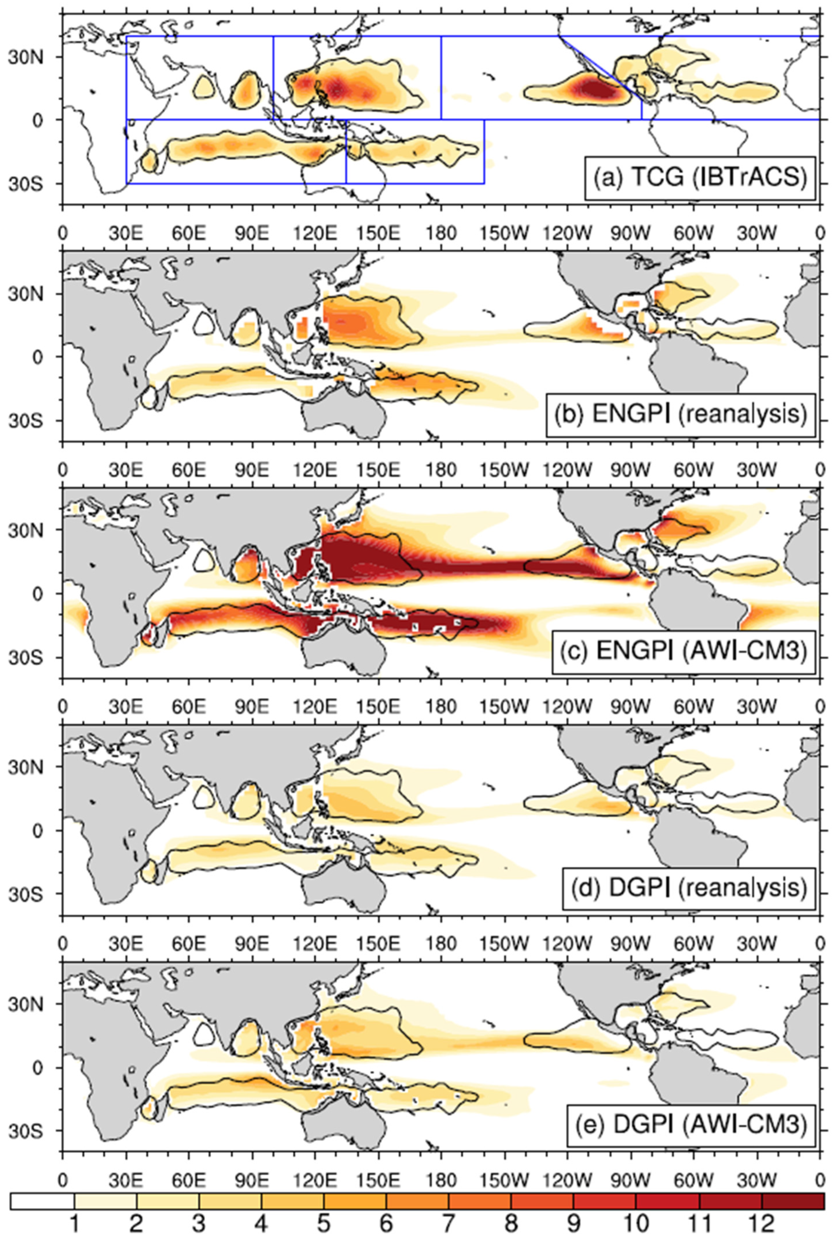
Figure 1 provides an overview of the climatological distributions of TCG from IBTrACS and the corresponding genesis potential diagnosed by ENGPI and DGPI from both the reanalysis and AWI-CM3. Observed TCG (Figure 1a) is concentrated primarily over the Western North Pacific (WNP), the North Indian Ocean (NIO), the Eastern North Pacific (ENP), the North Atlantic (NA), the South Indian Ocean (SIO), and the South Pacific (SP). These major genesis regions are well captured by both ENGPI (Figure 1b) and DGPI (Figure 1d) when computed from the reanalysis; this is expected, as GPIs are specifically formulated to reproduce the climatological distribution of TCG.
However, because GPIs are designed to provide a general representation of the global-scale TC-favorable environment, their ability to capture regional details is limited. Consequently, TCG over the ENP is underestimated, and the representation over the Arabian Sea is relatively weak in both indices (Figure 1b,d). AWI-CM3 broadly reproduces the large-scale spatial patterns of both ENGPI and DGPI (Figure 1c,e), but substantial regional biases are evident. In particular, the magnitude of ENGPI is systematically larger in AWI-CM3 than in the reanalysis, making it much stronger than implied by the observed IBTrACS TCG distribution. Moreover, the simulated ENGPI maximum over the ENP extends unrealistically into the Central North Pacific (CNP) (Figure 1c). For DGPI, although the overall magnitude is more comparable to the reanalysis and IBTrACS, an unrealistic center of TCG potential persists over the CNP (Figure 1e). These biases indicate deficiencies in the simulated large-scale environments governing TCG, which are examined in detail in the following section.

3.1.2. Attribution

To attribute biases in the GPI simulated by AWI-CM3 (relative to the reanalysis) to individual environmental factors, we apply a single-factor substitution method. Specifically, a pseudo-GPI is computed by replacing one term at a time with its AWI-CM3 value while holding all other terms fixed at their reanalysis values. The difference between this pseudo-GPI and the reanalysis-based GPI is then interpreted as the contribution of the bias from that specific term. It is important to note that because GPIs are nonlinear and multiplicative, the diagnosed contributions depend on the background state and do not necessarily sum exactly to the total GPI bias; the residual reflects nonlinear interactions among the different terms. These nonlinear interactions primarily arise from the cross-multiplication of thermodynamic and dynamic anomalies (e.g., simultaneous biases in mid-tropospheric humidity and vertical wind shear). While this method provides a first-order approximation of individual contributions, the inherent uncertainties mean that the derived contributions should be interpreted as relative weights rather than exact, independent physical forcings.
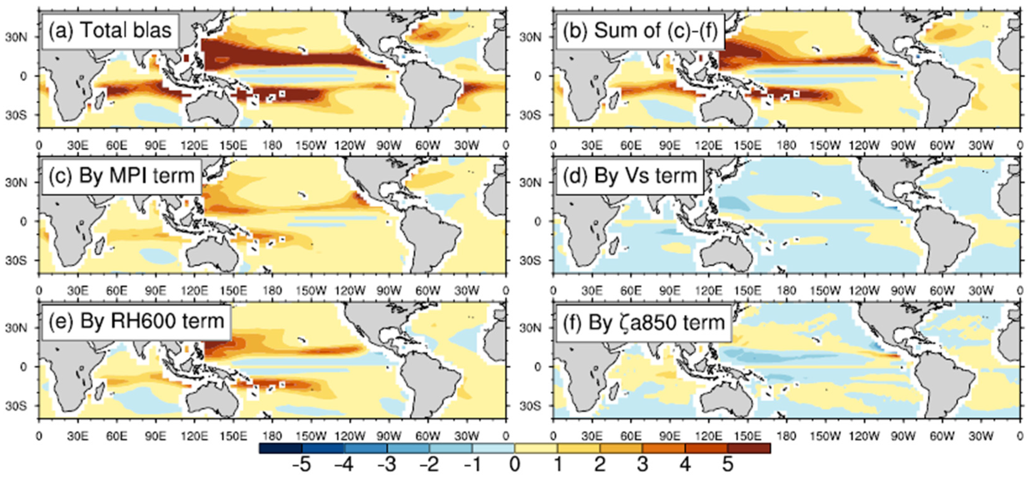
The contributions of individual terms to the ENGPI bias are decomposed and shown in Figure 2. As previously noted, the total ENGPI bias is characterized by a widespread positive bias, with particularly strong overestimation over the tropical Pacific. Among the four contributing terms, biases in MPI and RH600 terms dominate the overall ENGPI bias. Importantly, however, their spatial structures differ markedly: the MPI term bias is concentrated primarily over the ENP, whereas the RH600 term bias is strongest over the WNP. This contrast indicates that the ENGPI overestimation arises from different physical sources in different regions. In comparison, the contributions from Vs and ζa850 terms are substantially weaker and exhibit less spatial coherence. Notably, the sum of the four individual term contributions closely reproduces the total ENGPI bias, implying that nonlinear interactions among the ENGPI components are relatively small.
The MPI, which depends on the thermodynamic state of both the atmosphere and the underlying ocean, is fundamentally derived from the Carnot heat engine framework for tropical cyclones. In this theory, the square of the maximum wind speed (i.e., the kinetic energy) is proportional to the available thermodynamic energy extracted from the ocean–atmosphere system. Accordingly, MPI2 can be approximated as:
MPI2 = (CK/CD) × ((TS − T0)/T0) × (h*0 − h*)
where CK and CD are the surface enthalpy and momentum exchange coefficients, respectively; TS is the SST; T0 is the outflow temperature; h*0 is the saturation moist static energy at the sea surface; h* is that of the free troposphere. The factor (TS − T0)/T0 represents the thermodynamic efficiency of the TC heat engine, while h*0 − h* measures the thermodynamic disequilibrium between the ocean surface and the overlying atmosphere. Taking the natural logarithm of Equation (3) allows MPI to be decomposed into contributions from the thermodynamic efficiency and thermodynamic disequilibrium terms:
2 × log(MPI) = log(CK/CD) + log((TS − T0)/T0) + log(h*0 − h*).
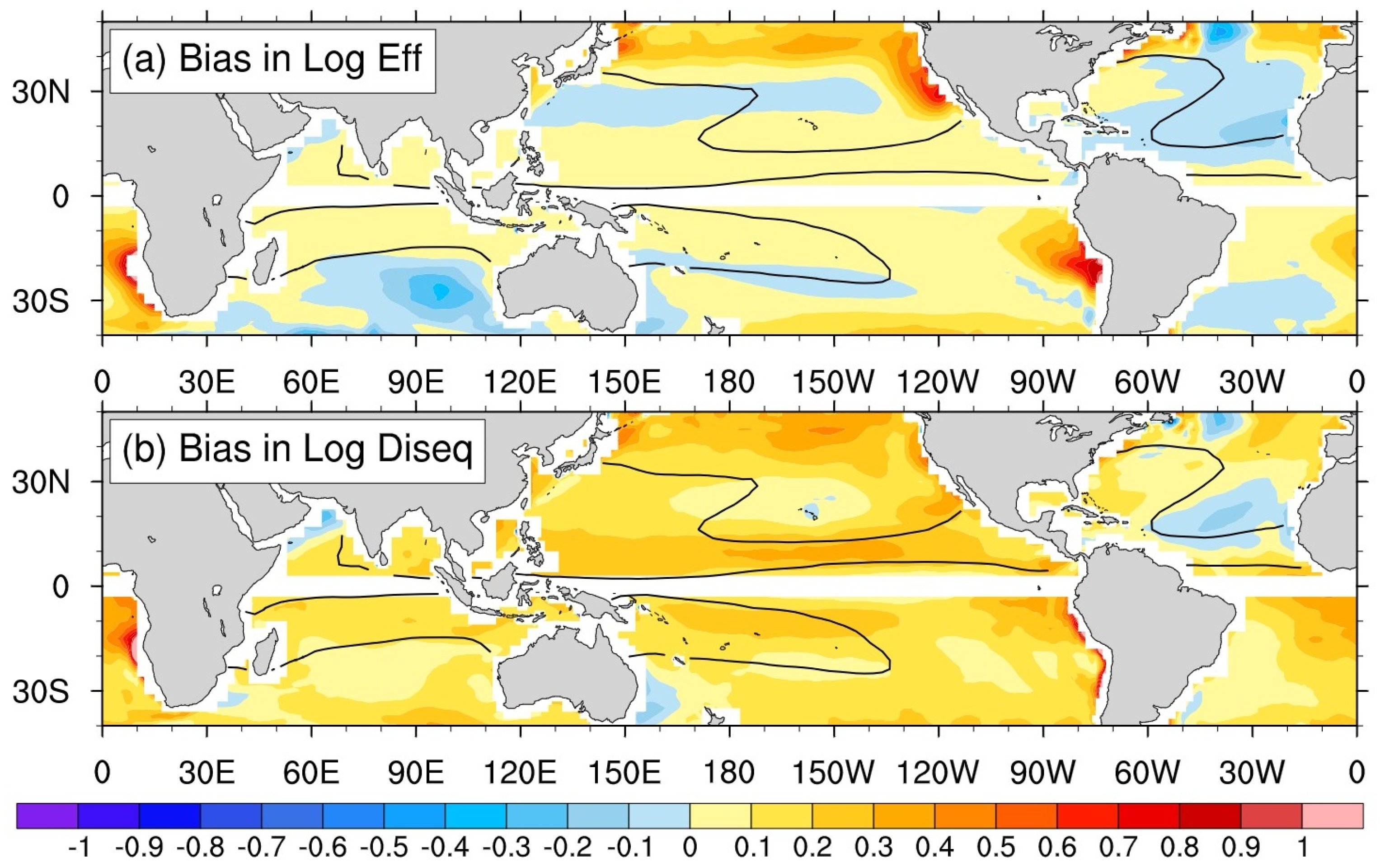
Therefore, to diagnose the sources of the MPI bias, Figure 3 shows the biases in the logarithms of the thermodynamic efficiency and thermodynamic disequilibrium terms defined in Equation (4). The bias in the thermodynamic efficiency term (Figure 3a) exhibits a complex spatial structure, with negative anomalies over the mid-latitude Pacific and the NA, and positive anomalies over the low- and high-latitude Pacific. In regions where thermodynamic efficiency is overestimated (underestimated), AWI-CM3 simulates air–sea conditions that are more effective at converting surface heat input into mechanical energy, thereby increasing the contribution of surface fluxes to MPI. The bias in the thermodynamic disequilibrium term (Figure 3b) shows a more spatially coherent signal, characterized by a widespread positive anomaly over most ocean basins. This indicates that AWI-CM3 systematically overestimates the thermodynamic contrast between the ocean surface and the overlying atmosphere, leading to excessively strong surface enthalpy fluxes and enhanced energetic support for TC development relative to the reanalysis. Overall, the MPI bias in AWI-CM3 is dominated by the thermodynamic disequilibrium term. While thermodynamic efficiency contributes regionally, the spatially coherent and predominantly positive disequilibrium bias provides the primary source of MPI overestimation and consequently the ENGPI bias.
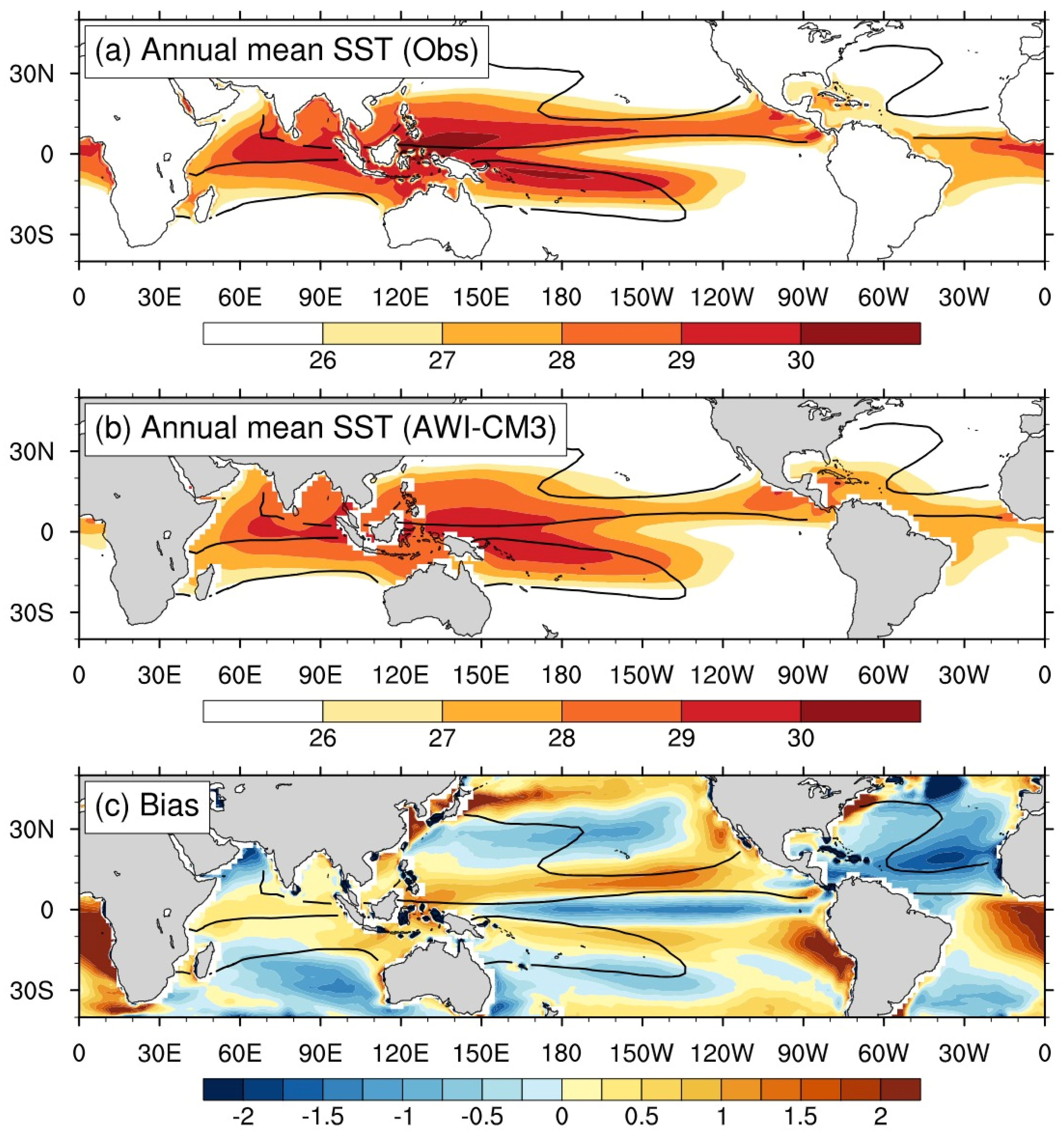
Both the thermodynamic efficiency and disequilibrium biases are closely tied to biases in the modeled sea surface conditions (Equation (4)). Although AWI-CM3 reproduces the broad-scale climatological annual mean SST distribution, it exhibits a pronounced equatorial Pacific cold tongue that extends too far west (Figure 4a,b) and is excessively cold (Figure 4c) relative to observations. This cold-tongue bias is a well-known systematic error in many coupled climate models [3]. Previous evaluations of CMIP6 models have consistently shown that excessive equatorial Pacific cold tongues and double-ITCZ biases are pervasive across the ensemble, and AWI-CM3’s performance in this regard is quantitatively comparable to other state-of-the-art models, indicating that these thermodynamic errors are widespread structural challenges rather than model-specific artifacts. The associated strengthening of the trade winds transports warm water from the eastern Pacific into the off-equatorial Pacific and warm pool over the WNP, leading to warm SST biases in those regions. In contrast, the NA exhibits a cold SST bias, likely related to a weak Atlantic Meridional Overturning Circulation (AMOC) (i.e., a colder NA coupled with a warmer South Atlantic), another common model deficiency [23]. The spatial pattern of SST biases closely resembles that of the thermodynamic efficiency bias, indicating that SST errors are a primary driver of the simulated efficiency anomalies.
SST biases can also affect the thermodynamic disequilibrium term by modulating surface enthalpy fluxes (Equation (3)), resulting in an overall correspondence between the two. Notably, regions characterized by strong warm SST biases generally show large positive biases in the thermodynamic disequilibrium term (Figure 3 and Figure 4). Nevertheless, this correspondence is not strict. For instance, over the NA and subtropical WNP, a cold SST bias coexists with an enhanced thermodynamic disequilibrium term. As visually evident in Figure 4c, these regional SST biases vary distinctly across the primary TC basins, with broad warm anomalies dominating the WNP, ENP, NIO, SIO, and SP, while the NA is characterized by a widespread cold anomaly. A possible explanation is that a cold SST bias tends to cool the overlying atmospheric column, which enhances the negative bias in saturation specific humidity aloft. Consequently, the negative bias in saturation moist static energy above the boundary layer can exceed that at the surface, resulting in a positive bias in the thermodynamic disequilibrium term and a larger MPI.
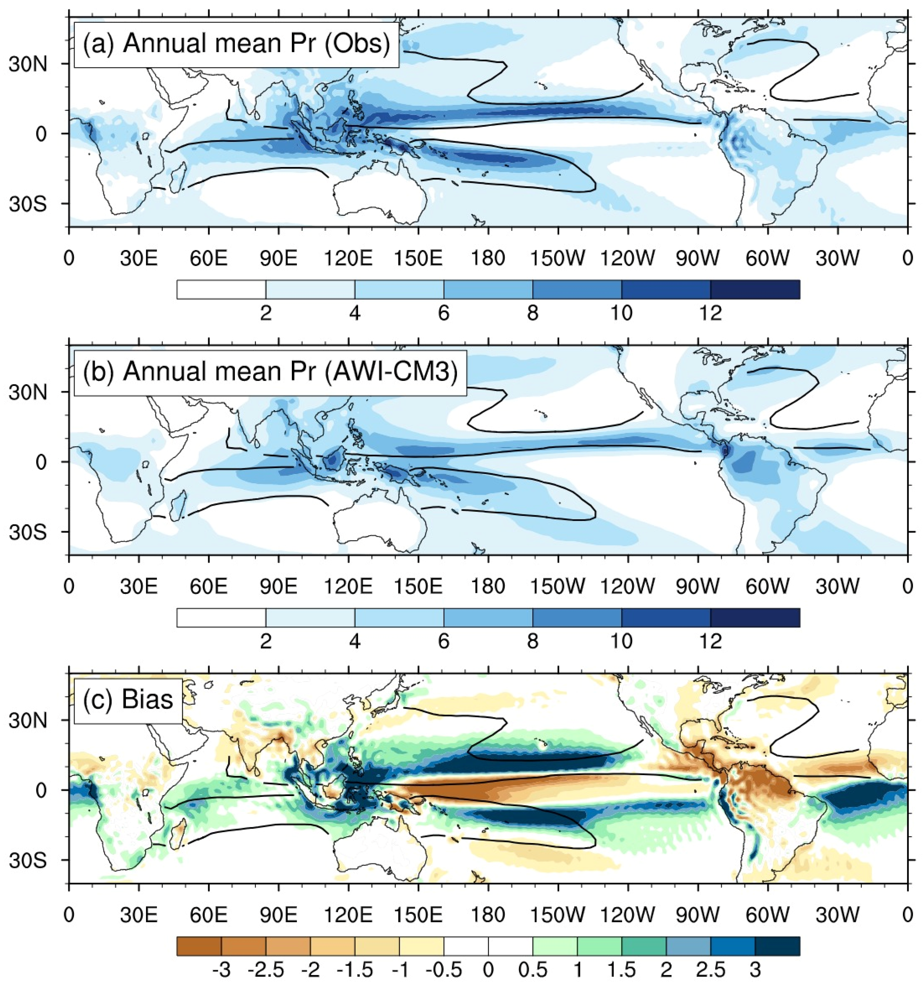
The RH600 bias, the other dominant contributor to the ENGPI bias, is likewise closely linked to SST errors (Figure 5). In association with the warm SST biases over the WNP warm pool and the off-equatorial Pacific, AWI-CM3 produces excessive equatorial precipitation, particularly over the Pacific, a manifestation of the well-known “double-ITCZ” problem [3]. This excessive precipitation is accompanied by overly active deep convection, which moistens the mid-troposphere and leads to the widespread positive relative humidity bias that strongly amplifies ENGPI (Figure 2).
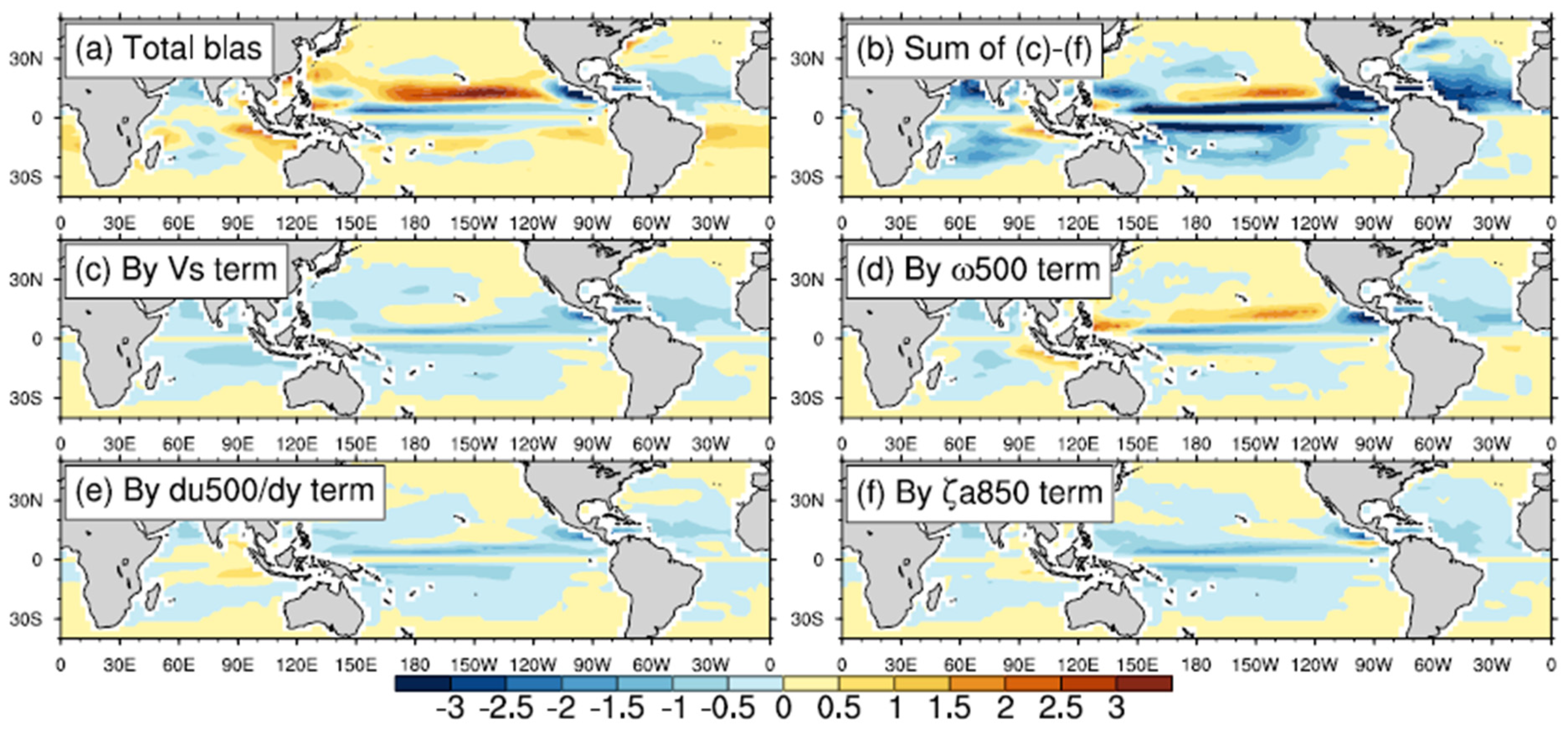
In contrast to the globally overestimated ENGPI, the bias of DGPI exhibits a more localized spatial structure (Figure 6). In the simulations, DGPI primarily overestimates TCG over the CNP and the Maritime Continent, while it is generally underestimated over the remaining ocean basins. When decomposed into contributions from individual dynamical factors, the overestimation of TCG in the equatorial region is found to be dominated by biases in the ω500 term within AWI-CM3, where anomalous ascent corresponds to an environment favorable for TCG.
The biases in the other three terms (i.e., Vs, du500/dy, and ζa850 terms) are generally consistent with the bias in the ω500 term, except in regions where positive ascend motion biases dominate. This coherence among these dynamical factors indicates that they are dynamically linked. As shown in Figure 4, biases in sea surface conditions are the primary driver of the vertical motion biases; specifically, warm SST biases enhance deep convection or suppress subsidence, leading to stronger ascent and a consequent overestimation of TCG, and vice versa. Meanwhile, the enhanced equatorial trade winds associated with an exaggerated zonal SST gradient strengthen the climatological zonal winds. This, in turn, increases the vertical wind shear, induces more negative relative vorticity, and enhances the meridional shear of the zonal wind. Together, these effects account for the generally underestimated DGPI over most of the Pacific basin.

3.2. Seasonal Cycle

3.2.1. Evaluation

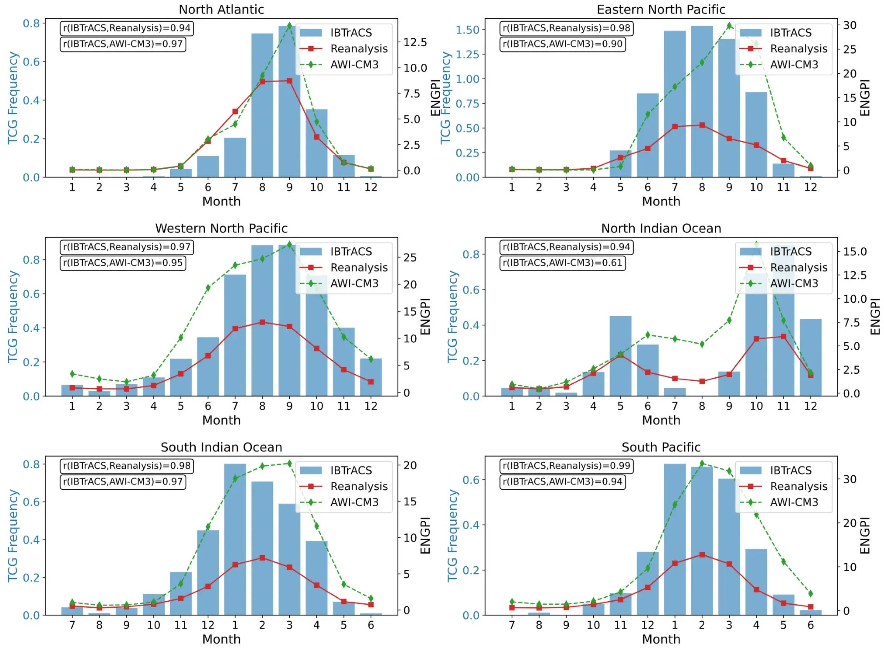
Beyond the annual mean state, a critical test for any climate model is its ability to reproduce the seasonal cycle of TCG [4]. This subsection evaluates how well AWI-CM3 captures the seasonal cycle of TCG frequency across primary global TC basins. In Figure 7, we compare the monthly observed TCG frequency with ENGPI derived from both the reanalysis and AWI-CM3 to assess the model’s ability to reproduce the seasonal timing and amplitude of TC-favorable conditions.
In terms of phase, the observed and simulated ENGPI perform very well, with correlation coefficients with observed TCG based on IBTrACS exceeding 0.90 in most ocean basins, except for the NIO. This indicates that AWI-CM3 realistically captures the seasonal transition into and out of TC-favorable environments, including the late-summer to early-autumn peak in the Northern Hemisphere and the austral-summer peak in the Southern Hemisphere. However, although the timing of the TC season is well simulated, AWI-CM3 systematically produces a higher magnitude of TC-favorable conditions than the reanalysis. The ENGPI values simulated by AWI-CM3 are substantially larger than those derived from the reanalysis in all seasons, often exceeding them by more than a factor of two. As discussed in Section 3.1, this overestimation arises from thermodynamic biases, particularly overly moist mid-tropospheric humidity and an overestimated MPI for storm intensity. These unrealistic environmental conditions lead to an exaggerated ENGPI, particularly during the peak TC season.
The NIO exhibits the weakest model performance. Over this basin, the observed TCG frequency shows a pronounced bimodal structure, with peaks during the pre-monsoon (May) and post-monsoon (November) seasons. This bimodal behavior is well captured by the reanalysis-based ENGPI, which shows a high correlation of 0.94 with observed TCG. In contrast, although AWI-CM3 also reproduces a bimodal seasonal cycle, the timing of the peaks is shifted: the pre-monsoon maximum occurs later than observed (June), while the post-monsoon peak appears earlier (October), leading to a lower correlation of 0.61 with observed TCG.
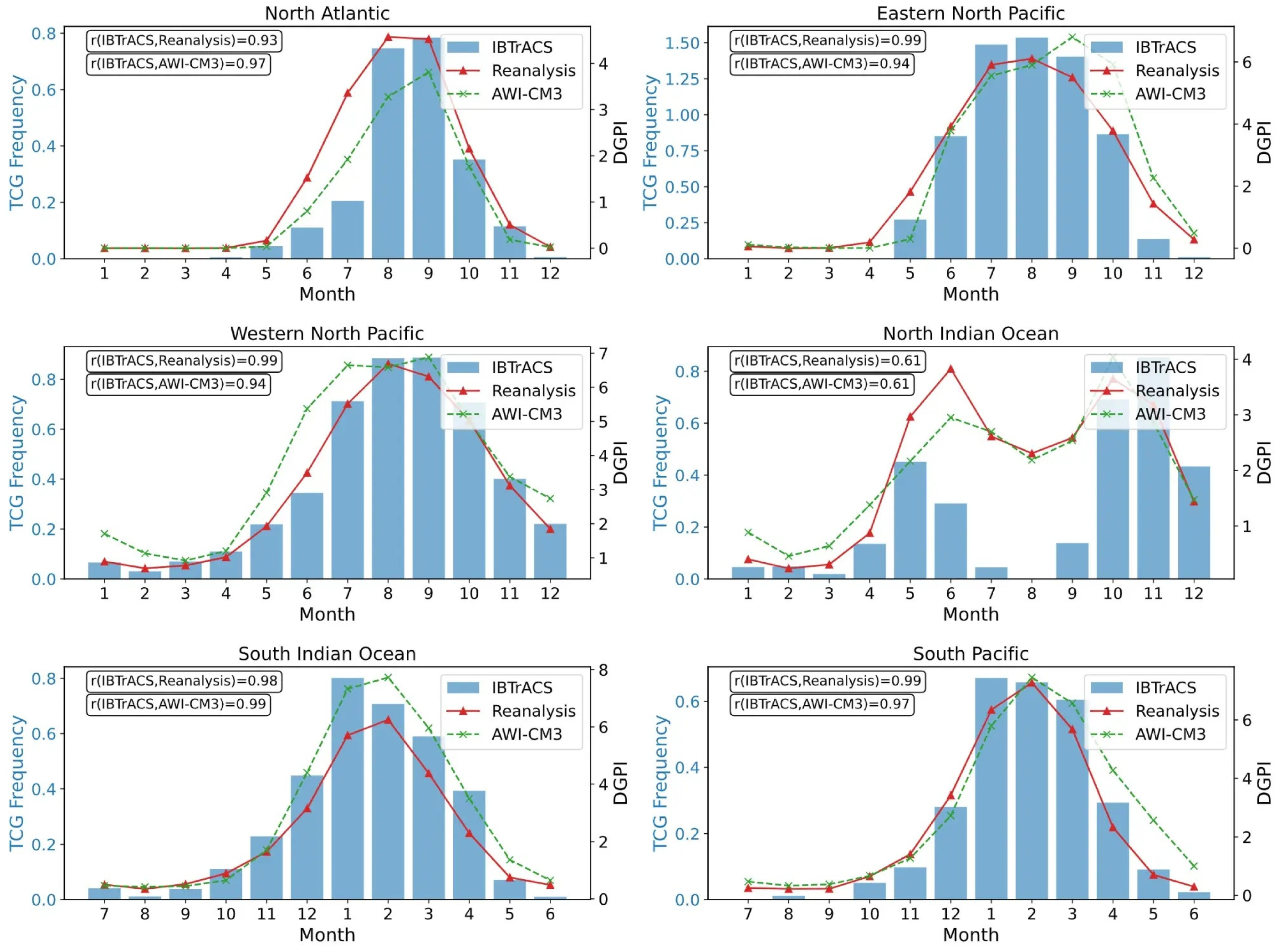
Figure 8 shows the corresponding seasonal cycle for DGPI. Similarly to ENGPI, DGPI reproduces the seasonal phase of TCG remarkably well in most basins, with correlation coefficients between observed TCG and DGPI, either based on reanalysis and simulation data, ranging from 0.93 to 0.99. Moreover, the amplitude of simulated DGPI closely follows that inferred from reanalysis, indicating that AWI-CM3 accurately captures the seasonal evolution of the dynamical conditions favorable for TC formation. The strong performance of DGPI is consistent with the results in Section 3.1, which demonstrate that AWI-CM3 simulates the large-scale dynamical environment more realistically than the thermodynamic environment.
The only basin in which DGPI shows reduced skill is again the NIO. Both the reanalysis-based and AWI-CM3-simulated DGPI exhibit systematic timing biases over the NIO, with the pre-monsoon peak occurring too late and the post-monsoon peak occurring too early. As a result, the correlations between DGPI and observed TCG are only 0.61 for both datasets. This consistency suggests that the DGPI error may not be primarily due to model biases or data uncertainty, but instead reflects a structural limitation of the DGPI itself. A possible explanation is that the NIO, characterized by a unique monsoon-related bimodal TC season, possesses dynamical controls on TCG that differ fundamentally from those in other basins. Consequently, a DGPI formulation based on globally uniform dynamical relationships may be unable to adequately represent TCG in this region.

3.2.2. Attribution

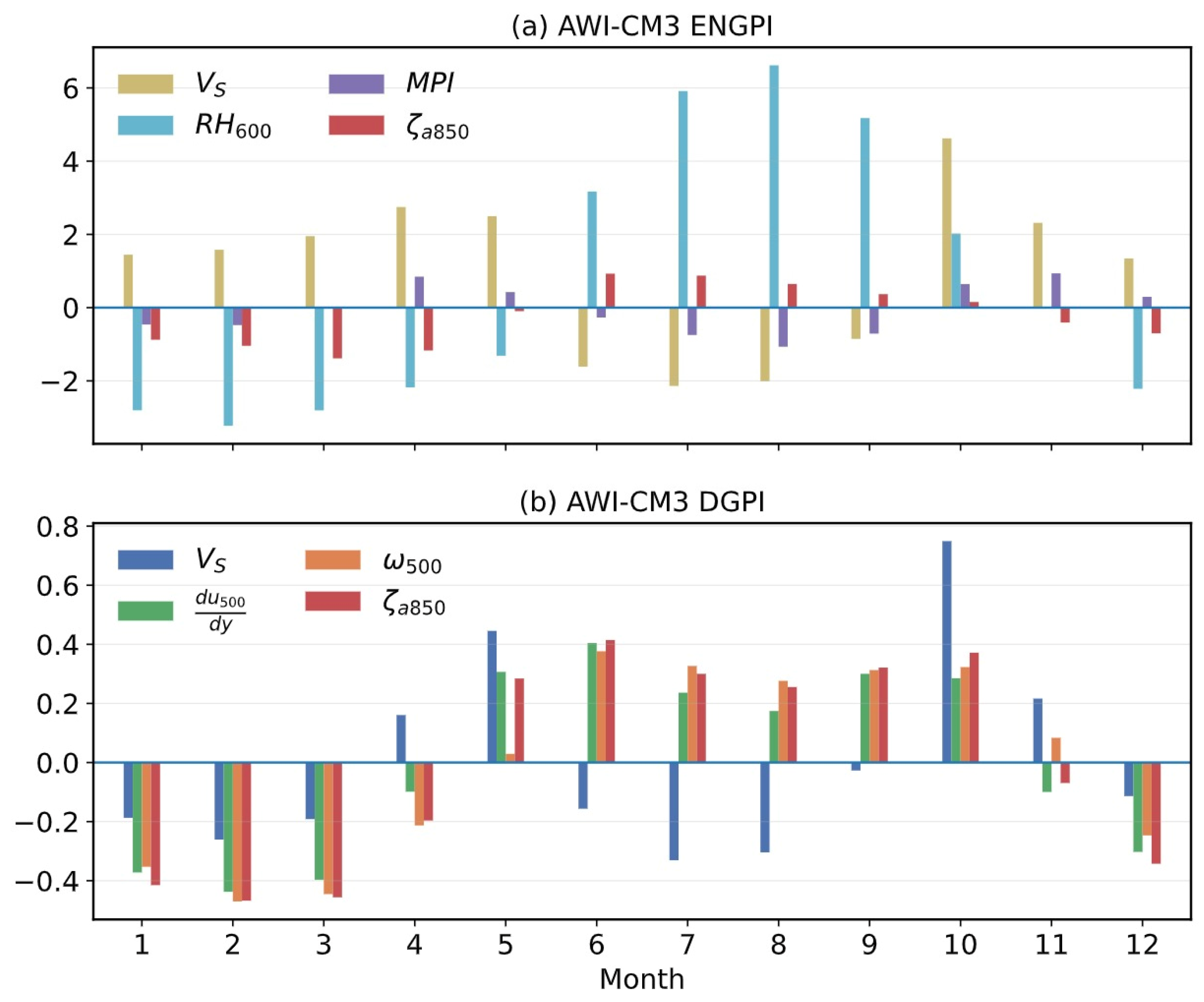
Given that AWI-CM3 exhibits its most pronounced biases over the NIO, we conducted a detailed investigation into this specific region. Similarly to the decomposition of annual mean GPI biases, the seasonal cycle of GPIs is attributed to individual environmental factors based on the single-factor replacement method. It is noted that a pseudo-GPI is computed by allowing one term to vary according to its seasonal cycle while all other terms are held fixed at their annual mean values. The difference between this pseudo-GPI and the annual mean GPI is then interpreted as the contribution of that term to the seasonal cycle. The decomposition results for ENGPI and DGPI over the NIO in AWI-CM3 are shown in Figure 9.
For the ENGPI simulated by AWI-CM3, the seasonal cycle is dominated primarily by the RH600 term. During the boreal summer, the development of the South Asian Summer Monsoon (SASM) enhances deep convection and precipitation over the NIO, substantially moistening the mid-troposphere. This produces high RH600 that strongly favors TCG. Concurrently, the SASM is dynamically characterized by low-level westerlies and upper-level easterlies, which generate strong Vs, a suppressor of TC development. Thus, RH600 and Vs exert opposing influences on ENGPI throughout the year. In contrast, MPI and ζa850 terms contribute little to the seasonal cycle of ENGPI.
Observationally, TCG over the NIO is strongly suppressed during the SASM season, indicating that Vs dominates over RH600 in controlling cyclogenesis. However, in AWI-CM3, although TCG also exhibits a bimodal seasonal cycle, TCG remains unrealistically high during the SASM period. This suggests that the model overestimates the positive effect of RH600, implying excessively strong simulated convection and humidity conditions associated with the SASM. Furthermore, AWI-CM3 produces an abnormally large ENGPI in October, primarily driven by the signal from Vs, which is inconsistent with observations. This behavior indicates that the model fails to represent the seasonal retreat of the SASM, leading to a distorted large-scale circulation and erroneous environmental controls on TCG.
Regarding DGPI, the contributions from individual factors are relatively comparable, and no single term dominates the seasonal cycle. During the non-monsoon season, all four factors tend to vary in the same direction, jointly suppressing TCG. In contrast, during the monsoon season, the behavior of these terms becomes inconsistent. Although the Vs term continues to exert a negative influence on TC formation, the other three factors (ζa850, du500/dy, and ω500 terms) simultaneously provide positive contributions of comparable or larger magnitude. This synchronized behavior originates from the tight dynamical coupling of these variables within the SASM circulation. During the monsoon season, enhanced deep convection and low-level convergence intensify large-scale ascent; the development of the monsoon trough increases low-level vorticity; simultaneously, the meridional zonal wind shear also strengthens. Their combined effect overwhelms the inhibiting role of Vs, causing DGPI to misinterpret a strong monsoon background as a highly favorable TC-forming environment. In October, the strong Vs signal again dominates, producing a secondary DGPI peak that appears earlier than in observations, similar to the bias seen in ENGPI.

3.3. Interannual Variability

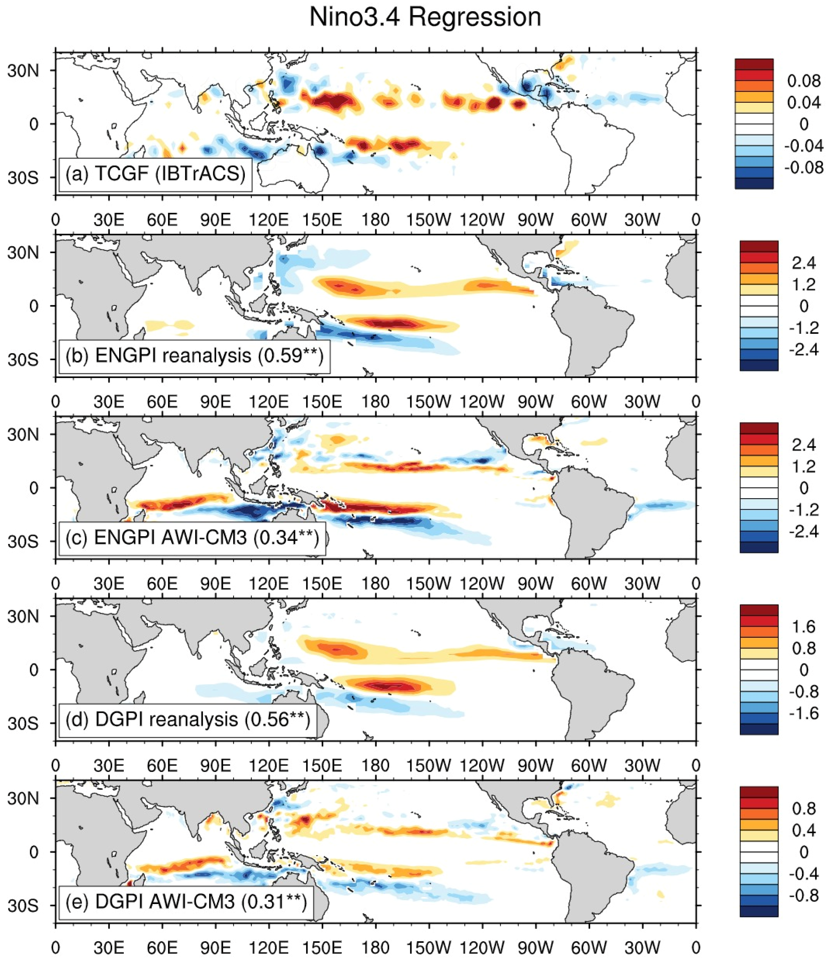
For the interannual variability of TCG, we focus specifically on the modulation by ENSO, which significantly impacts TC behavior worldwide [8]. For instance, during El Niño episodes, TC activity generally declines in the NA and the far WNP, but rises in the central and ENP [9]. Hence, a reliable metric for evaluating a climate model’s accuracy is its capacity to replicate the observed influence of ENSO on TCG potential. This subsection assesses how well AWI-CM3 represents year-to-year variations in TCG potential linked to the Niño 3.4 index.
Figure 10 illustrates the spatial patterns of TCG, ENGPI, and DGPI projected onto the Niño 3.4 index for both IBTrACS and those estimated from GPIs. In observations, ENSO shows a clear and physically coherent relationship with TCG. During El Niño events, TCG is significantly enhanced over the central Pacific and ENP and suppressed over the WNP near the East Asian coast and the Maritime Continent. This reflects the eastward displacement of deep convection and the Walker circulation. This ENSO–TCG pattern is well captured by the ENGPI in the reanalysis, with a high pattern correlation (cc = 0.59, p < 0.01). This indicates that the large-scale environmental controls embedded in ENGPI faithfully translate ENSO-induced circulation changes into TCG interannual variability. The simulated ENGPI reproduces a similar ENSO-related structure, albeit with a reduced pattern correlation (cc = 0.34, p < 0.01). Meanwhile, although the observed DGPI still shows an ENSO-related variability with a reasonable pattern correlation (cc = 0.56, p < 0.01), it fails to reproduce the reduced TCG over the WNP near the East Asian coast. The simulated DGPI is also capable of reproducing the ENSO signal on TCG (cc = 0.31, p < 0.01), close to its performance of ENGPI.
However, remarkable biases persist across both the observed and simulated GPI interannual variability related to ENSO. For example, GPIs tend to miss the relationship between ENSO and TCG over the tropical NA. For the GPIs in the reanalysis, they show less influence of ENSO on TCG over the SIO. Conversely, the simulated GPIs exhibit an excessively strong positive ENSO–TCG relationship over the tropical SIO, which may be the primary reason for their lower correlation relative to reanalysis-based GPIs. Furthermore, the similarity between biases in the ENSO signal within ENGPI and DGPI, whether in the reanalysis or AWI-CM3, indicates that these biases may be caused by the same terms in both GPIs, namely the dynamical factors such as Vs and ζa850. Physically, the lower spatial correlations in the model simulations compared to the reanalysis stem from AWI-CM3’s tendency to produce a more westward-extended and narrowly confined ENSO SST anomaly pattern. This structural SST bias alters the Walker circulation response, leading to displaced anomalies in vertical wind shear and low-level vorticity over the western Pacific and Indian Ocean, which ultimately degrades the spatial fidelity of the simulated GPI response to ENSO.

4. Conclusions

This study systematically evaluates the performance of the AWI-CM3 climate model in reproducing the large-scale environmental conditions favorable for TCG, as diagnosed by the ENGPI and DGPI. By comparing historical simulations against reanalysis and observed TCG frequency, we assessed the model’s fidelity in capturing the climatological annual mean state, seasonal cycle, and interannual variability related to ENSO.
First, AWI-CM3 broadly reproduces the global spatial distribution of TCG potential but exhibits significant regional biases. The ENGPI is systematically overestimated globally, particularly over the tropical Pacific, primarily due to thermodynamic errors. Excessive mid-tropospheric relative humidity and an overestimation of MPI are the dominant drivers, which are closely linked to the model’s SST and “double-ITCZ” biases. In contrast, the DGPI bias is more localized and shows a more realistic magnitude, as the model’s dynamical fields are simulated with higher fidelity than the thermodynamic fields. Second, the model demonstrates high skill in capturing the seasonal phase of TCG potential across most basins. However, the NIO remains a challenging region for both GPIs. In the NIO, AWI-CM3 fails to precisely represent the bimodal peak timing and overestimates TC-favorable conditions during the SASM season. The persistence of these timing errors in both reanalysis and simulated DGPI suggests a structural limitation of the index itself in representing the unique monsoon-driven dynamics of the NIO. Finally, AWI-CM3 successfully replicates the interannual modulation of TCG potential by ENSO, capturing the characteristic pattern of enhanced TCG potential in the central/eastern Pacific and suppressed potential in the western Pacific during El Niño years. Although the correlation between ENSO and simulated GPIs is lower than that of the reanalysis, the model faithfully translates ENSO-induced circulation changes into variations in TCG potential.
In summary, AWI-CM3 demonstrates robust performance as a high-quality climate model, faithfully replicating the fundamental characteristics of observed TCG and associated potential. Meanwhile, our evaluation highlights that while both ENGPI and DGPI perform exceptionally well across multiple timescales, they possess distinct limitations that must be carefully considered in future climate projections. For ENGPI, the simulated magnitude is heavily dependent on thermodynamic components. In a warming world, the projected increase in thermodynamic variables, such as sea surface temperature and mid-tropospheric humidity, may lead to an unrealistic, exaggerated intensification of ENGPI. Consequently, for future TCG potential analyses based on ENGPI, it may be more appropriate to employ a relative threshold rather than an absolute value. Conversely, the primary challenge for DGPI lies in the tight dynamical coupling among its constituent factors. While this interdependence reflects the integrated nature of large-scale circulations like the SASM, it simultaneously precludes a multifaceted perspective for examining TCG potential. Meanwhile, because these variables evolve so closely in tandem within the model, it becomes nearly impossible to isolate the independent contribution of any single dynamical driver. Furthermore, the persistent biases identified in the NIO suggest that GPI-based assessments of future TC peak timing and seasonal shifts in this basin should be interpreted with caution. These findings provide a critical perspective for optimizing the use of GPIs to reduce uncertainty in future projections of TCG. Specifically, researchers utilizing these indices for future climate assessments should avoid relying solely on absolute GPI values, particularly for ENGPI, and instead employ relative anomaly thresholds to mitigate the artificial inflation driven by systematic thermodynamic biases. For the NIO and similar monsoon-dominated regions, future projections based on existing GPI formulations must be treated with extreme caution, and we strongly recommend the development of basin-specific or dynamically adaptive indices that can better capture complex regional circulation changes under greenhouse warming.

Author Contributions

Conceptualization, B.A.S. and J.S.; methodology, J.S. and J.Z.; software, J.Z.; validation, B.A.S. and J.S.; formal analysis, B.A.S. and J.S.; investigation, B.A.S. and J.S.; resources, J.S.; data curation, J.S.; writing—original draft preparation, B.A.S.; writing—review and editing, J.S. and B.A.S.; visualization, J.S.; supervision, J.S.; project administration, J.S.; funding acquisition, J.S. All authors have read and agreed to the published version of the manuscript.

Funding

This research was funded by the National Natural Science Foundation of China, grant number 42088101.

Institutional Review Board Statement

Not applicable.

Informed Consent Statement

Not applicable.

Data Availability Statement

The data presented in this study are available on request from the corresponding author.

Conflicts of Interest

The authors declare no conflicts of interest.

References

  1. Walsh, K.J.E.; McBride, J.L.; Klotzbach, P.J.; Balachandran, S.; Camargo, S.J.; Holland, G.; Knutson, T.R.; Kossin, J.P.; Lee, T.; Sobel, A.; et al. Tropical cyclones and climate change. WIREs Clim. Change 2016, 7, 65–89. [Google Scholar] [CrossRef]
  2. World Meteorological Organization. WMO Atlas of Mortality and Economic Losses from Weather, Climate and Water Extremes (1970–2019); WMO-No. 1267; WMO: Geneva, Switzerland, 2021. [Google Scholar]
  3. Van Oldenborgh, G.J.; Van Der Wiel, K.; Sebastian, A.; Singh, R.; Arrighi, J.; Otto, F.; Haustein, K.; Li, S.; Vecchi, G.; Cullen, H. Attribution of extreme rainfall from Hurricane Harvey, August 2017. Environ. Res. Lett. 2017, 12, 124009. [Google Scholar] [CrossRef]
  4. Shan, K.; Yu, X. Seasonal advance of intense tropical cyclones in a warming climate. Nature 2023, 623, 83–89. [Google Scholar] [CrossRef] [PubMed]
  5. Bell, S.S.; Chand, S.S.; Tory, K.J. Using historical tropical cyclone climate datasets to examine the role of observational uncertainty on trend detection. Sci. Rep. 2022, 12, 11612. [Google Scholar] [CrossRef] [PubMed]
  6. Landsea, C.W.; Harper, B.A.; Hoarau, K.; Knaff, J.A. Can we detect trends in extreme tropical cyclones? Science 2006, 313, 452–454. [Google Scholar] [CrossRef] [PubMed]
  7. Torn, R.D.; Snyder, C. Uncertainty of tropical cyclone best-track information. Weather Forecast. 2012, 27, 715–729. [Google Scholar] [CrossRef]
  8. Vecchi, G.A.; Knutson, T.R. Estimating annual numbers of Atlantic hurricanes missing from the HURDAT database (1878–1965) using ship track density. J. Clim. 2011, 24, 1736–1746. [Google Scholar] [CrossRef]
  9. Gray, W.M. Hurricanes: Their formation, structure and likely role in the tropical circulation. In Meteorology over the Tropical Oceans; Royal Meteorological Society: Bracknell, UK, 1979; pp. 155–218. [Google Scholar]
  10. DeMaria, M.; Knaff, J.A.; Connell, B.H. A tropical cyclone genesis parameter for the tropical Atlantic. Weather Forecast. 2001, 16, 219–233. [Google Scholar] [CrossRef]
  11. Emanuel, K.; Nolan, D.S. Tropical cyclone activity and the global climate system. In Proceedings of the 26th Conference on Hurricanes and Tropical Meteorology, Miami, FL, USA, 3–7 May 2004; pp. 240–241. [Google Scholar]
  12. Wang, B.; Murakami, H. Dynamic genesis potential index for diagnosing present-day and future global tropical cyclone genesis. Environ. Res. Lett. 2020, 15, 114008. [Google Scholar] [CrossRef]
  13. Roberts, M.J.; Camp, J.; Seddon, J.; Vidale, P.L.; Hodges, K.; Vannière, B.; Mecking, J.; Haarsma, R.; Bellucci, A.; Scoccimarro, E.; et al. Impact of model resolution on tropical cyclone simulation using the HighResMIP–PRIMAVERA multimodel ensemble. J. Clim. 2020, 33, 2557–2580. [Google Scholar] [CrossRef]
  14. Camargo, S.J.; Emanuel, K.A.; Sobel, A.H. Use of a genesis potential index to diagnose ENSO effects on tropical cyclone genesis. J. Clim. 2007, 20, 4819–4834. [Google Scholar] [CrossRef]
  15. Wehner, M.F.; Reed, K.A.; Li, F.; Prabhat; Bacmeister, J.; Chen, C.-T.; Paciorek, C.; Gleckler, P.J.; Sperber, K.R.; Collins, W.D.; et al. The effect of horizontal resolution on simulation quality in the Community Atmospheric Model, CAM5.1. J. Adv. Model. Earth Syst. 2014, 6, 980–997. [Google Scholar] [CrossRef]
  16. Murakami, H.; Vecchi, G.A.; Underwood, S. Patterns and frequency of projected future tropical cyclone genesis are governed by dynamic effects. Commun. Earth Environ. 2022, 3, 77. [Google Scholar] [CrossRef]
  17. Moon, J.Y.; Streffing, J.; Lee, S.S.; Semmler, T.; Andrés-Martínez, M.; Chen, J.; Dorn, F.; Haak, H.; Hempel, S.; Hinrichs, C.; et al. Earth’s future climate and its variability simulated at 9 km global resolution. Earth Syst. Dyn. 2025, 16, 1103–1134. [Google Scholar] [CrossRef]
  18. Streffing, J.; Sidorenko, D.; Semmler, T.; Zampieri, L.; Scholz, P.; Andrés-Martínez, M.; Cao, N.; Cuevas, E.; Danilov, S.; Dorn, F.; et al. AWI-CM3 coupled climate model: Description and evaluation experiments for a prototype post-CMIP6 model. Geosci. Model Dev. 2022, 15, 6399–6427. [Google Scholar] [CrossRef]
  19. Hersbach, H.; Bell, B.; Berrisford, P.; Hirahara, S.; Horányi, A.; Muñoz-Sabater, J.; Nicolas, J.; Peubey, C.; Radu, R.; Schepers, D.; et al. The ERA5 global reanalysis. Q. J. R. Meteorol. Soc. 2020, 146, 1999–2049. [Google Scholar] [CrossRef]
  20. Kanamitsu, M.; Ebisuzaki, W.; Woollen, J.; Yang, S.; Hnilo, J.J.; Fiorino, M.; Potter, G.L. NCEP–DOE AMIP-II reanalysis (R-2). Bull. Am. Meteorol. Soc. 2002, 83, 1631–1643. [Google Scholar] [CrossRef]
  21. Gelaro, R.; McCarty, W.; Suárez, M.J.; Todling, R.; Molod, A.; Takacs, L.; Randles, C.A.; Darmenov, A.; Bosilovich, M.G.; Reichle, R.; et al. The Modern-Era Retrospective Analysis for Research and Applications, Version 2 (MERRA-2). J. Clim. 2017, 30, 5419–5454. [Google Scholar] [CrossRef] [PubMed]
  22. Knapp, K.R.; Kruk, M.C.; Levinson, D.H.; Diamond, H.J.; Neumann, C.J. The International Best Track Archive for Climate Stewardship (IBTrACS). Bull. Am. Meteorol. Soc. 2010, 91, 363–376. [Google Scholar] [CrossRef]
  23. Wang, C.; Zhang, L.; Lee, S.K.; Wu, L.; Mechoso, C.R. A global perspective on CMIP5 climate model biases. Nat. Clim. Change 2014, 4, 201–205. [Google Scholar] [CrossRef]
Figure 1. Climatological annual mean distributions of (a) observed TCG frequency from IBTrACS (in number of genesis events per year at each 2.5° × 2.5° grid box), (b) ENGPI from reanalysis, (c) ENGPI from AWI-CM3, (d) DGPI from reanalysis, and (e) DGPI from AWI-CM3 for the period 1980–2017. In each panel, the black contour encloses regions where the plotted value exceeds 1.5. Blue boxes in (a) indicate the six primary TC basins analyzed in this study.
Atmosphere 17 00369 g001
Figure 2. Decomposition of the climatological annual mean ENGPI bias (AWI-CM3 minus reanalysis): (a) total bias, (b) sum of individual term contributions (cf), (c) MPI term, (d) Vs term, (e) RH600 term, and (f) ζa850 term.
Atmosphere 17 00369 g002
Figure 3. Biases in the logarithms of the MPI decomposition terms (AWI-CM3 minus reanalysis): (a) thermodynamic efficiency term (log Eff) and (b) thermodynamic disequilibrium term (log Diseq). Black contours indicate 1 for the climatological annual mean ENGPI from reanalysis.
Atmosphere 17 00369 g003
Figure 4. Climatological annual mean SST (°C) from (a) observations and (b) AWI-CM3, and (c) the SST bias (AWI-CM3 minus observations). In each panel, the black contour indicates the climatological annual mean ENGPI value of 1 from the reanalysis, delineating the primary regions of TC genesis potential.
Atmosphere 17 00369 g004
Figure 5. Climatological annual mean precipitation (mm day−1) from (a) observations, (b) AWI-CM3, and (c) the precipitation bias (AWI-CM3 minus observations). In each panel, the black contour indicates the climatological annual mean ENGPI value of 1 from the reanalysis, delineating the primary regions of TC genesis potential.
Atmosphere 17 00369 g005
Figure 6. Same as Figure 2, but for the DGPI bias decomposition: (a) total bias, (b) sum of individual term contributions (cf), (c) Vs term, (d) ω500 term, (e) du500/dy term, and (f) ζa850 term.
Atmosphere 17 00369 g006
Figure 7. Seasonal cycle of observed TCG frequency (blue bars) and ENGPI from reanalysis (red solid) and AWI-CM3 (green dashed) across six primary basins.
Atmosphere 17 00369 g007
Figure 8. Same as Figure 7, but for DGPI.
Atmosphere 17 00369 g008
Figure 9. Decomposition of the seasonal cycle of (a) ENGPI and (b) DGPI over the North Indian Ocean in AWI-CM3 into contributions from individual terms.
Atmosphere 17 00369 g009
Figure 10. Regression of (a) observed TCG frequency, and (be) ENGPI and DGPI from reanalysis and AWI-CM3 onto the Niño 3.4 index. Pattern correlations are in parentheses; double asterisks denote 99% significance.
Atmosphere 17 00369 g010
Disclaimer/Publisher’s Note: The statements, opinions and data contained in all publications are solely those of the individual author(s) and contributor(s) and not of MDPI and/or the editor(s). MDPI and/or the editor(s) disclaim responsibility for any injury to people or property resulting from any ideas, methods, instructions or products referred to in the content.