Article

Evaluation of a Community Monitoring Network for Improved Characterization of PM2.5 Exposure in Fresno County, California, USA


1
Department of Life and Environmental Sciences, School of Engineering, University of California, Merced, CA 95348, USA
2
Department of Public Health, School of Social Sciences, Humanities and Arts, University of California, Merced, CA 95348, USA
3
Central California Asthma Collaborative, Fresno, CA 93727, USA
4
Stockton Unified School District, Stockton, CA 95206, USA
5
Health Sciences Research Institute, University of California, Merced, CA 95348, USA
*
Authors to whom correspondence should be addressed.
Atmosphere 2026, 17(2), 187; https://doi.org/10.3390/atmos17020187
Submission received: 9 December 2025 / Revised: 29 January 2026 / Accepted: 7 February 2026 / Published: 11 February 2026
(This article belongs to the Section Air Quality and Health)

Abstract

Air quality in the San Joaquin Valley (SJV) often fails to meet Environmental Protection (EPA) Standards for particulate matter (PM) ≤ 2.5 microns. The San Joaquin Valley Center for Air Injustice Reduction (SJV-CAIR) at the University of California, Merced, partnered with local community-based organizations to expand networks of low-cost air quality monitors (PurpleAir, PA-II) in Fresno County to increase community air monitoring to better characterize air pollution trends and spatial variability. In this study, we compared community and regulatory air pollution monitoring using PM2.5 data from the SJV-CAIR network in Fresno County during June–July 2023. Measurements from community monitors identified locations across the county that may episodically exceed National Ambient Air Quality Standards (NAAQS) compared with regulatory monitors, while providing similar concentration estimates. Our study also compared characterization of spatial variability in PM exposure using interpolation maps with only regulatory monitors and the enhanced community monitoring network. These analyses identified four weeks with increased PM2.5 concentrations in some locations that were not identified by regulatory monitors. These findings indicate that low-cost community sensors can be an effective tool for supplementing regulatory monitoring to provide localized PM2.5 exposure information to residents and, importantly, identify high-risk areas that warrant ongoing assessment using approved regulatory monitors.

1. Introduction

California’s San Joaquin Valley (SJV) has some of the worst air quality in the United States (US) for particulate matter (PM) [1]. The SJV is an inland California valley that extends south from Stockton to Bakersfield, California and is bounded by the Sierra Nevada mountains to the east and coastal ranges to the west. This topography, combined with local climate conditions and regional pollution sources, creates an environment conducive to air pollution formation and retention [2]. Air quality in the SJV often fails to meet Environmental Protection (EPA) Standards for Particulate Matter 2.5 (PM2.5), which are particles less than 2.5 μm in diameter.
Short-term health effects of PM2.5 exposure include asthma, wheezing, shortness of breath, coughing, and chest discomfort and pain [3]. Long-term exposure to PM2.5 can lead to premature death, emergency department (ED) visits, hospital admission, asthma attacks, chronic bronchitis, cancer, cardiovascular disease, and diabetes [4]. In the US, PM2.5 has decreased across most of the country from 1988 to 2016. However, PM2.5 has increased in wildfire-prone areas such as the SJV [5], which is adjacent to heavily forested mountains. The SJV has some of the highest rates of asthma and ED visits and hospitalizations for respiratory illness in California [6,7]. Previous studies indicate that ozone levels in this region typically increase during the spring, summer, and fall, while PM2.5 values increase during the fall and winter. Thus, there is very little relief for residents from poor air quality [8].
Historically, PM2.5 measurements have been reported from regulatory monitoring stations, operated by the federal or local governments, utilizing BAM (Beta Attenuation Monitoring) or other technologies. In the SJV, regulatory monitors are sparsely located and may provide less accurate air quality information to residents living away from the monitors, especially in rural locations. These deficiencies are largely due to variations in air quality due to differences in hyper-local emission sources and meteorology that are outside regulatory monitors’ spatial range [9]. Thus, increased density of monitors could increase characterization of PM2.5 spatial variability and exposure and identify locations with higher exposures and potential health impacts. However, regulatory monitors are costly to set up (~$30,000+) and maintain (requiring monthly site servicing by a qualified technician). As an alternative, low-cost sensor-based monitors can increase local PM monitoring [10,11] and expand access to hyper-local air pollution information. However, with the rise of low-cost monitoring, concerns about the reliability, robustness, and accuracy of these systems have been raised [12].
Although data are subject to sensor and environment-related limitations, prior work shows that quality assurance protocols like calibration and correction frameworks, network-level quality control, and systematic sensor placement strategies can substantially improve data reliability [13,14,15,16,17,18]. Previous studies have successfully used low-cost citizen science monitors to examine PM worldwide, with studies demonstrating their use for community monitoring, exposure assessment, and identification of localized pollution patterns [17,19,20,21,22,23,24]. These studies are often focused on urban areas with high concentrations and polluted environments [24,25,26]. Additionally, recent publications have successfully used PurpleAir (Draper, Utah, USA) and other low-cost PM2.5 sensors in epidemiologic and exposure science. For example, one study in Brazil demonstrated that PurpleAir data predicted respiratory hospitalizations and captured wildfire-associated variability in air quality [27]. In broader exposure modeling contexts, low-cost sensors across the country have been used to relate PM2.5 concentrations and monitor distribution to socioeconomic status, epidemiology studies, and woodsmoke-impacted environments [28,29,30,31,32,33,34]. In California, there has been substantial government investment in community-based air monitoring initiatives such as statewide low-cost sensor deployment programs, community air grants, and initiatives under Assembly Bill 617 [35]. However, comparisons on a local scale have not been assessed to confirm accuracy within largely rural and suburban communities like the SJV.
The San Joaquin Valley Center for Air Injustice Reduction (SJV-CAIR) at the University of California, Merced, is working to address these concerns by expanding a local network of low-cost calibrated PurpleAir (PA-II) monitors across the SJV (https://www.sjvair.com, accessed on 14 August 2022). This network, like others across the state, is one of the largest community air monitoring networks in the US that uses additional calibration techniques to ensure data quality [36,37].
In this study, we evaluated whether utilizing measurements from community air monitors improved the spatial resolution of air quality exposure compared to solely relying on regulatory monitors. To address this question, we compared PM2.5 measurements in Fresno County from community monitors to measurements by regulatory monitors for a 2-month period. We also examined differences in spatially interpolated PM2.5 exposure maps across the county when incorporating the enhanced community monitoring network. This approach allowed us to assess how sensor density and new placements influence the ability to characterize spatial variability in air pollution.

2. Materials and Methods

2.1. Establishing the SJV-CAIR Monitor Network and Data Collection

2.1.1. Study Area

Fresno County is located in the central SJV, ~15,500 km2 in area, and home to ~1,000,000 residents [38] (Figure S1). Our study region focused on Fresno County, CA and is bounded by 35.9–37.6° N and 118.4–120.9° W. This region includes additional monitors placed outside the county lines to obtain more precise PM2.5 estimates at the county borders. There were 18 regulatory-grade monitors, 257 privately purchased PurpleAir monitors and 47 calibrated PurpleAir monitors included in the study (Table S1). The region is semi-arid with hot summers and cool winters. Pollution sources in the SJV include traffic-related air pollutants (TRAP) from the Interstate 5 and Highway 99 [39] transportation corridors, agricultural production, rail, other industries, periodic wildfires, and pollution advected from dense coastal cities.

2.1.2. Fresno County Monitor Placements

The PurpleAir monitors used in this study draw air through a laser-based sensor (Plantower, Nanchang, China) and apply standard algorithms set by the manufacturer to estimate PM2.5 concentrations from light scatter (Supplemental Information S1) [40,41]. Our community partner, Central California Asthma Collaborative (CCAC), has developed additional QA/QC and calibration methods to ensure high-quality data [42]. Briefly, SJV-CAIR monitors are calibrated PurpleAir monitors that were calibrated for 7–28 days in groups of 30–40 against a constant federal reference method (FRM) monitor to ensure accuracy for PM2.5 values exceeding 35 μg/m3, the 24 h National Ambient Air Quality Standards (NAAQS) for PM2.5. Calibration focused on higher concentrations because accurate measurements at elevated levels are critical for health-relevant exposure assessment. Data from the monitors was then analyzed to generate intra-device (A vs. B sensor) and inter-device (monitor 1 vs. monitor 2) correlations and variance. Acceptable monitors demonstrated intra- and inter-device correlations greater than 0.98 and average variance less than 10%.
Previous field studies for low-cost sensors reported overestimates at elevated relative humidity (RH) levels (above 70–80%) [43,44,45,46,47], likely due to the hygroscopic growth of particles, ref. [48] reinforcing the need for correction models in deployments [46,47,49,50]. However, our data did not suggest overestimation under these conditions and performed consistently across the range of observed RH during field deployment. This conclusion was similarly confirmed by an analysis from the South Coast Air Quality Management District (SCAQMD), which reported that laboratory temperature and relative humidity minimally effect the sensors’ results [51,52].
To ensure continued reliable PM2.5 concentrations, the SJVAir network calculates intra-device correlations (A vs. B particle counts) on an ongoing basis for each new data entry to ensure internal sensor consistency. Additionally, 18 calibrated PurpleAir monitors, previously tested and validated by the SJVAir team, are collocated with regulatory grade monitors operated by the San Joaquin Valley Air Pollution Control District, the California Air Resources Board (CARB), and SJVAir at locations across the SJV. These 18 collocated monitors are used to generate daily calibration equations that are applied to non-collocated community monitor data based on proximity to each collocated site. These equations correct for sensor bias and improve agreement across all community monitors in the network, supporting the reliability of our PM2.5 measurement [42]. Three of these collocated monitors are in Fresno County (Figure S5A). During 2023, median percent differences between collocated community and regulatory monitors in Fresno County ranged from 9.0% to 22.2%, corresponding to a difference of about 2.4–5.8 µg/m3 (Figure S5B). The correlation of the community sensors with their respective collocated regulatory-grade monitors was 0.93, 0.97, and 0.69, with all p-values < 0.001. Correlations were highest during weeks with elevated PM2.5, indicating that the low-cost sensors captured higher-exposure events effectively. Overall, these results fall within the range reported for well-calibrated low-cost PM2.5 sensors and demonstrate that calibration through collocated reference instruments improves cross-network consistency [53,54].
Prior to this study, there were 428 PurpleAir monitors in the SJVAir community monitoring network (SJVAir.com). This network gathers data from all publicly available PurpleAir monitors in the SJV, including those subjected to CCAC’s QA/QC procedures described above. An additional 44 SJV-CAIR calibrated PurpleAir monitors were installed between January 2023 and July 2023 in Fresno, Stanislaus, and San Joaquin counties to increase coverage in underserved areas. Monitors were usually installed in homes, businesses, fire stations, and schools on the side of a building (under the eaves), approximately 8 feet off the ground.
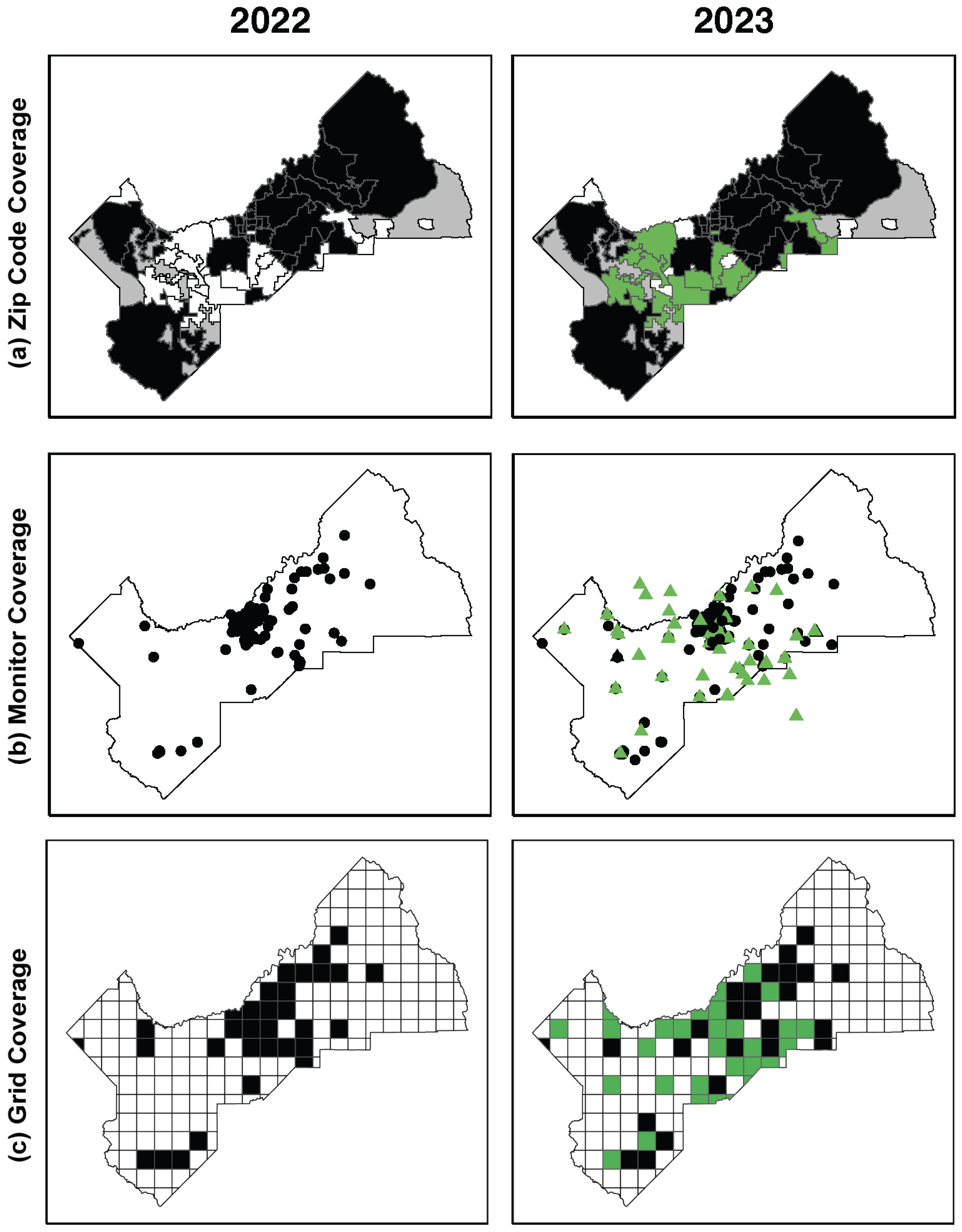
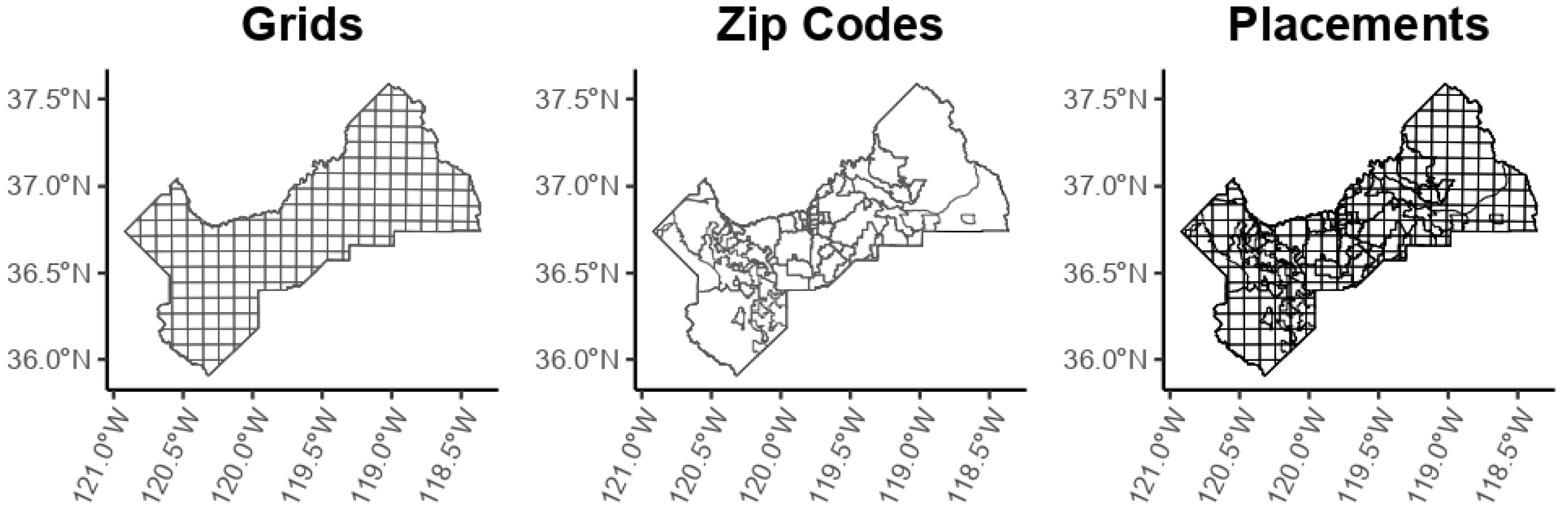
The SJV-CAIR monitors were placed with community partners across the SJV using a grid–zip code system (Figure 1) to assure longevity and accuracy of data collection. The selection of SJV-CAIR monitor placements had two priorities: (1) having at least one monitor in every zip code to pair with zip code-level county health data and, (2) expanding coverage to improve uniform geographic placement. A uniform grid was utilized alongside zip codes in the boundary area to provide placement suggestions. In Fresno County, this uniform grid was composed of 200 square cells of size 100 km2.
Prior to placement, 176 of these 200 (88%) cells and 23 of the 55 Fresno zip codes (41.8%) were without monitors. After placement of 44 new monitors, 132 cells (66%) and 3 zip codes (5.5%) were monitor-less (Figure 2). While previous monitors were primarily close to the Fresno city center, our new SJV-CAIR monitors increased coverage for residents in more rural areas. All data from SJV-CAIR monitors are publicly available to provide accurate PM2.5 information to residents across the county.

2.1.3. Data Collection

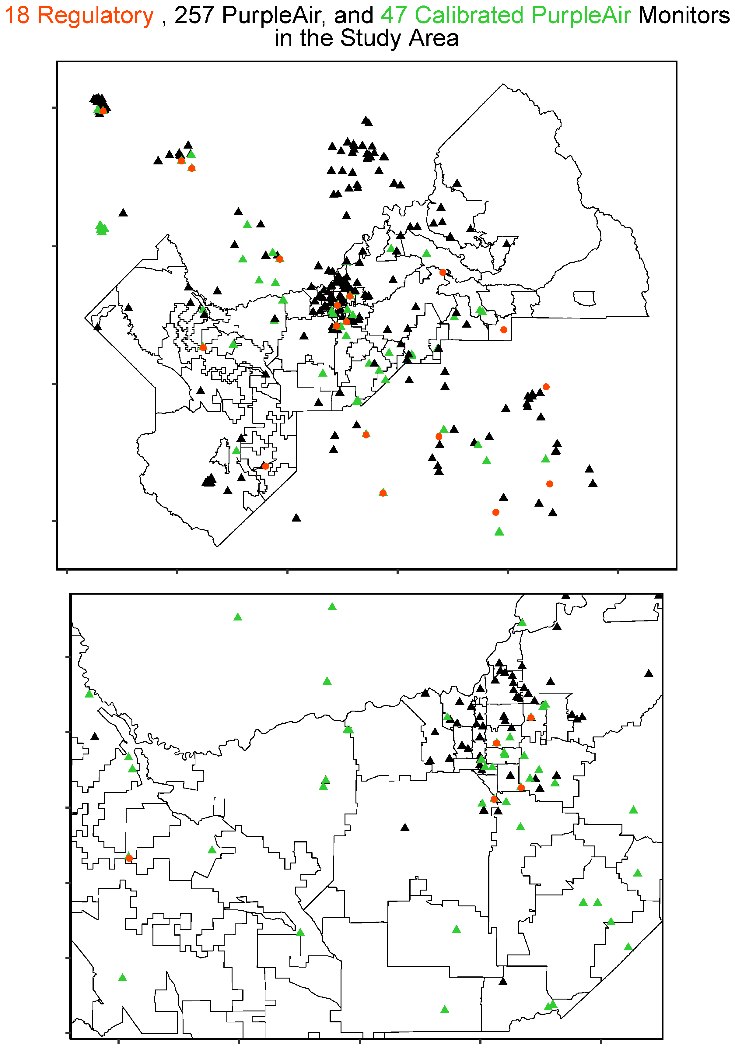
PM2.5 daily averages were downloaded from the SJVAir website for June and July 2023 and weekly averages were calculated (Supplemental Information S2). Previous studies used a similar two-month study to include a large amount of data but reduce seasonal and monitor variation [55,56]. Weekly estimates were selected to identify spatiotemporal trends that will match future studies looking at health outcomes. Negative PM values were imputed to zero because PurpleAir monitors can report negative values when readings are close or equal to zero. The data used in this study included 18 regulatory monitors (EPA, BAM1022), 257 PurpleAir monitors and 47 calibrated PurpleAir monitors within the study area (Figure 3). The calibrated PurpleAir monitors include the additional SJV-CAIR monitors we installed to augment the SJVAir network (Table S1). Thus, existing PurpleAir monitors and the calibrated PurpleAir monitors are denoted as community monitors in our analysis (Table S1).

2.2. Statistical Methods

Once all community monitors were deployed, we examined how the density and placement of the expanded network influenced spatial detection of PM2.5. We fitted Bayesian spatial regression models and model performance was evaluated using both prediction error (mean squared error) and the overlap of 95% credible intervals between community- and regulatory-based estimates. All statistical methods were conducted using R version 4.3.1 with R packages geoR and spBayes and coordinates used the WGS84 (EPSG 4326) projection.
Empirical semivariograms were constructed using the geoR package [57] to assess the spatial dependence of all our PM2.5 data by measuring the variability between data points as a function of distance. Semivariograms were fit for each week using both community and regulatory monitor weekly averages. While the exponential, Gaussian, spherical, and Matérn models were considered, we selected a Gaussian covariance function because it most accurately characterized the weekly correlation structure. Estimates of the decay parameter, nugget, and partial sill parameters from Gaussian empirical semivariograms were used as initial values for our spatial regression models. A directional Gaussian semivariogram was constructed as a sensitivity analysis to determine if there were unique spatial patterns in different directions (0, 45, 90, 135), which provided an assessment of anisotropy in each direction for weekly PM2.5 concentrations.
Bayesian spatial regression models with Gaussian covariance functions were employed using the spBayes package in R, as described by Finley et al. (2015) [58]. For each week, two models predicting PM2.5 concentrations were fit, one using community monitor readings and another using regulatory monitor readings. Individual priors, starting values, and tuning parameters for ϕ, τ2, and σ2 were assigned from our initial empirical semivariogram plots and updated via metropolis steps (Table S2). A sample of 10,000 Markov Chain Monte Carlo (MCMC) samples were taken from the posterior. Posterior means and 95% credible intervals were calculated for parameters of interest.
We used two approaches to assess the differences in county PM2.5 characterization between community and regulatory monitors. First, PM2.5 measurements produced by the regulatory monitors were compared to observed community monitor data. To accomplish this, for each weekly regulatory model fit at each community monitor location, samples were drawn from the posterior predictive distribution and means were constructed (the number of community monitor locations varied by week). Then, for each week, we compared the estimated mean PM2.5 concentration to the known weekly measurements at that community monitor location using the mean squared error (MSE) formula:
M S E = 1 n Σ ( x i y i ) 2
where n is number of observations, x i is the measured PM2.5 concentration at community monitor (i), and y i is the predicted regulatory PM2.5 value at the respective community monitor’s (i) location. Here, higher MSE values reflect a larger difference from the observed data, e.g., PM information that would be lost if only regulatory monitors were used to estimate PM data in the SJV.
Second, for every model described above, estimates at each of the 2128 gridded locations were drawn from the posterior predictive distributions. Corresponding means and 95% credible intervals (using the 2.5th and 97.5th percentile) were constructed for each of the 2128 gridded locations. Community and regulatory credible intervals were considered overlapping if the 2.5th percentile of one interval was smaller than the 97.5th of the other interval. The percentage of overlap between the community and regulatory monitor posterior samples was calculated at each gridded location.
We also determined the number of days the community and regulatory monitors measured PM2.5 exceeding NAAQS (>35 µg/m3 for 24 h averages) [59].

3. Results

3.1. Spatial Temporal Trends in Fresno County

3.1.1. Semivariogram Trends

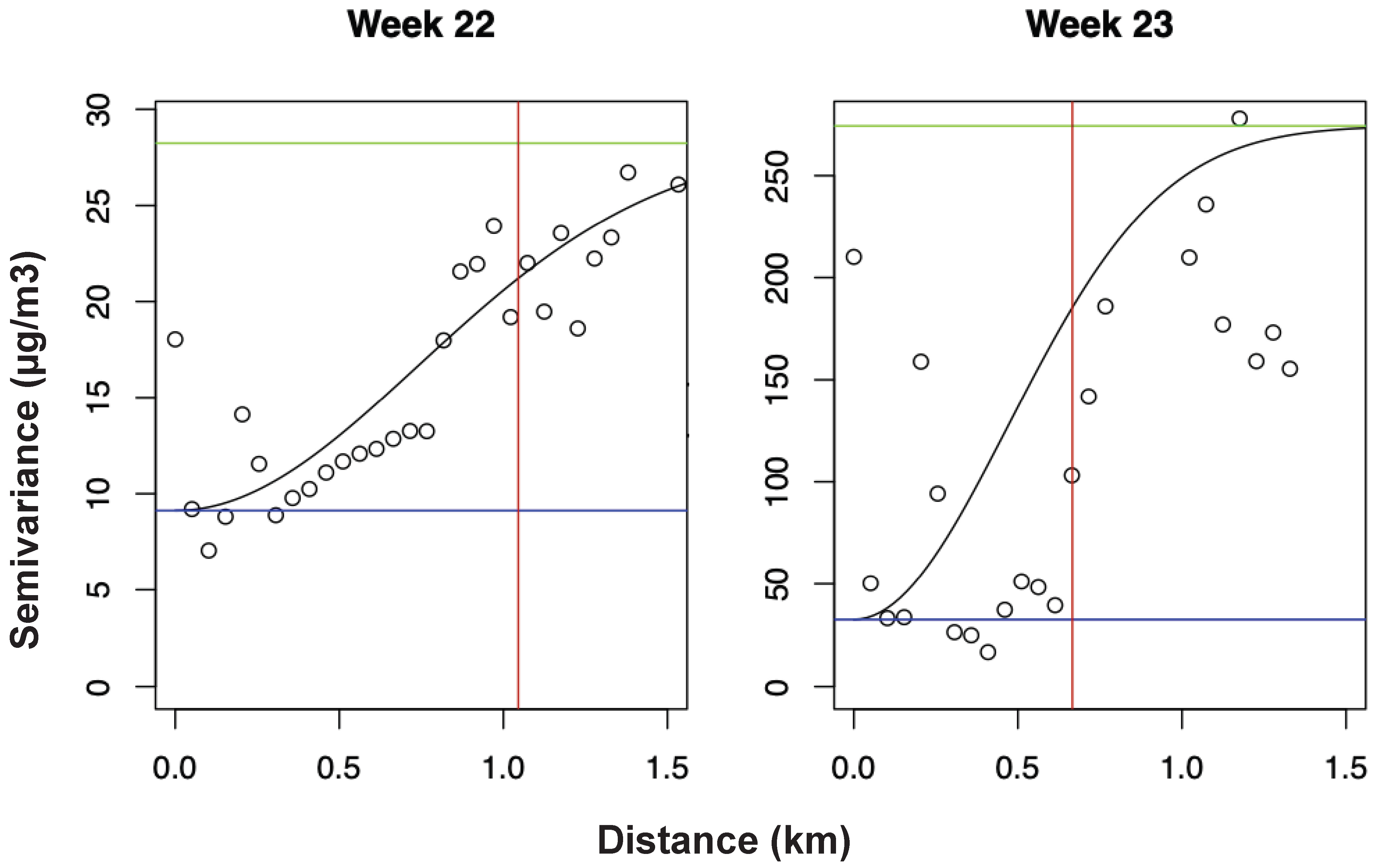
Table 1 presents semivariogram analysis for all sensors with a Gaussian model fit during each week using our starting values for the Gaussian spatial regression model. The decay parameter (ϕ) describes how quickly the correlation between two points declines as a function of distance. The nugget (τ2) and partial sill (σ2) are the non-spatial and spatial variances, respectively. All weeks except week 31 had a nugget ranging from 0.01 to 168.2, representing the small-scale variations or error in measurements. The decay parameters had similar values for all weeks, ranging from 0.34 to 0.66, corresponding to a spatial range (3/ϕ) of 4.5–8.8 km. However, the sill varied significantly between weeks that experienced high levels of PM2.5 (weeks 23, 29, 30, and 31) and weeks with lower PM2.5 levels (weeks 22, 24, 25, 26, and 27) (Figure 4). Figure 4 presents the difference between a low PM2.5 level (week 22) and a high PM2.5 concentration week (week 23). During week 22, the sill was equal to 28.2 while during week 23, a week with elevated PM2.5 levels, the sill increased to 274.3. Therefore, as expected, there was more variability between our data points on weeks with elevated PM2.5 levels.
These variograms provided valuable insight about the spatial variability of PM2.5 levels during our study period and helped inform the starting values for the computed surfaces, below. Specifically, the weekly variability in semivariograms indicates spatial and temporal differences between weekly PM2.5 concentrations. This finding suggests there were spatial differences between our high pollution and good air quality weeks. We conducted sensitivity analyses using directional semivariogram analysis for each week during the study period to examine the spatial dependence of PM2.5 levels in different directions. The directional semivariograms revealed some anisotropy in PM variability with 0/135 and 90/45 directions showing stronger associations.

3.1.2. Spatial Surface Trends

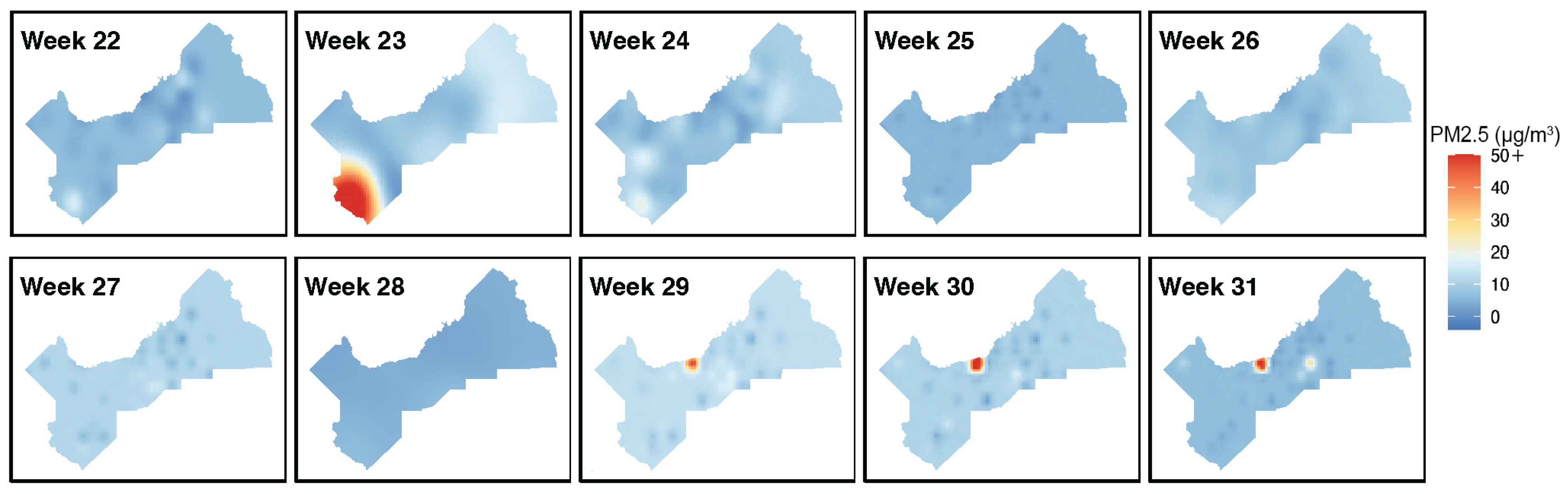
Weekly PM2.5 interpolation estimates (µg/m3) across Fresno County are plotted in Figure 5. Spatial temporal trends for the study period identified two locations across Fresno County that experienced elevated PM2.5 levels. Both locations exceeded the NAAQS 24 h PM2.5 standard of 35 µg/m3. During weeks 29, 30, and 31 there were elevated levels in North Central Fresno. This region is bounded by Highway 99 and is an agricultural area, both of which may contribute to elevated PM2.5 concentrations. For example, one community monitor located directly next to Highway 99, experienced 24 h average PM2.5 values of 140 µg/m3 during the two-month study (Table S3). Elevated PM2.5 levels were noted during week 23 in Southwest Fresno County near the town of Coalinga (Figure 5). Coalinga is a rural community with a population of approximately 13,380 in Southwest Fresno County. The town is surrounded by oil fields and is a large agricultural area, land uses that can result in high PM2.5 emissions. Land use may explain the elevated weekly PM2.5 levels and high daily averages in the area, with one Coalinga community monitor experiencing daily average values of 41.82 µg/m3 (Table S3). During other weeks (22, 24–28) of our study period, the PM2.5 levels were moderately low, which is the usual during the summertime in Fresno County when persistent northwest winds may dilute local pollution [60].

3.2. Monitor Type Comparisons Between Regulatory and Community Monitors

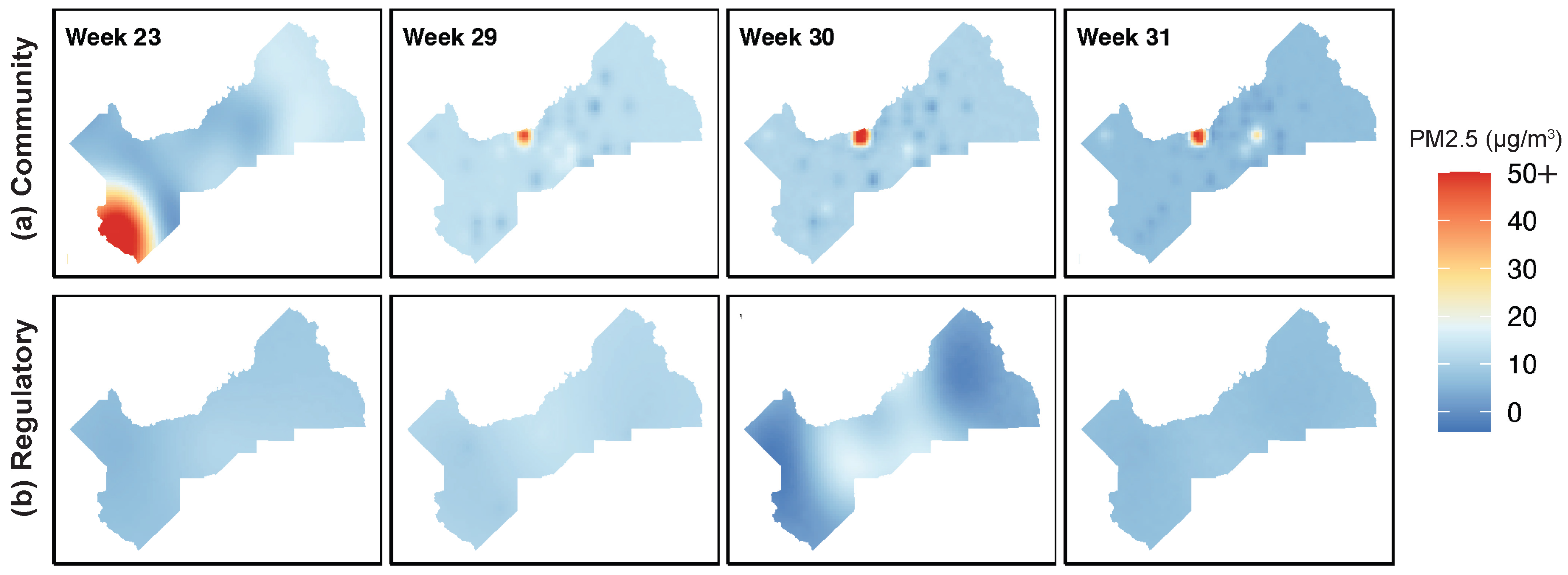
Figure 6 compares the kriged surface PM2.5 concentrations in Fresno County by monitor type. The interpolations display estimates of PM surfaces across Fresno County with the use of community monitors (Figure 6a) compared with data from just regulatory monitors (Figure 6b). During June and July, hotspots for PM2.5 exposure were identified in North Central and Southwest Fresno by community monitors with weekly averages reaching as high as 55 μg/m3 during weeks 23, 29, 30 and 31 (Figure 6a). Regulatory monitor interpolations did not identify these hotspots (Figure 6b), reporting values ranging from 0 to 10 μg/m3 during these weeks. Importantly, differences between our community and regulatory interpolation surfaces further suggested that regulatory monitors across the county did not identify high PM2.5 exposure weeks. Specifically, weeks 23, 30, and 31 reported differences ranging from 35 to 60 μg/m3 across the county. Additional analyses were conducted to determine if these hotspots were identified by SJV-CAIR monitors (Figure S4). While the additional SJV-CAIR monitors were strategically placed to improve spatial coverage, our analysis indicates that their inclusion did not lead to substantial changes in the overall characterization of PM2.5 spatial patterns compared to the pre-existing community network. We therefore interpret the new SJV-CAIR monitors’ primary contribution as improving network completeness and consistency rather than revealing new pollution hotspots or significantly altering exposure surfaces. Additionally, during the study period, community-based monitors identified 85 days that exceeded NAAQS; however, regulatory monitors did not identify any days. Note that concentrations of PM2.5 are naturally lower during the summer months due to differences in emissions and meteorology. Nevertheless, areas across Fresno County, specifically North Central and Southwest Fresno, still experienced high levels of PM2.5 during our study period.
This finding was supported by MSE computations comparing the regulatory monitor estimates and the actual measurements (a weekly average) at each community monitor. This analysis provided insight into how well new community monitors provided accurate PM2.5 concentrations across the county. If there was a large MSE, community monitors reported values regulatory monitors did not observe. Table 2 shows the MSE using the kriged Bayesian surface and community monitor measurements. Note that the highest MSEs were reported during weeks our community monitors identified hotspots (23, 29, 30, and 31). The high MSE reflects the increased observed differences in PM2.5 between community monitors and the more sparsely located regulatory monitors, which may miss localized peaks in PM2.5. The uncertainties in these values arise from the normal error associated with low-cost sensors, the sparse regulatory monitor spacing, and local-scale variability not captured by interpolation. This finding suggests community monitors were providing additional data not identified through the regulatory monitor network during our study period, especially on days with increased levels of PM2.5.
Additional analyses were conducted to analyze the average weekly 95% posterior credible interval (PCI) for the 10,000 regulatory and community monitor posterior samples at each of the 2128 gridded locations (Table 3). PCIs values were larger for the community monitors’ 97.5th percentile during six of the ten weeks. Also, community monitor PCIs tended to be wider; likely due to the larger number of community monitors in the study area (300 compared to 18 regulatory monitors), which provided a larger range of hyper-local data and therefore larger PCIs. Generally, the percentage of overlap between community and regulatory monitors was high, ranging from 79.8 to 99.7%. The lowest PCI occurred on hotspot week 23, reporting 79.8% overlap.

4. Discussion

We expanded a community air monitoring network in Fresno County, California, and found that more abundant low-cost air quality sensors are likely to better characterize PM2.5 exposure to local residents compared with sparser regulatory-grade monitors. Specifically, community monitors identified two locations (Southwest Fresno County and North Central Fresno County) with increased PM2.5 exposure during June–July 2023 that could not be identified using sparsely distributed regulatory monitors. These locations are in known agricultural areas and along a major transportation corridor that cuts through the SJV. We demonstrated these improvements in PM exposure estimation using interpolated PM2.5 maps. Fresno County has eight regulatory-grade monitors within its boundaries, while 2000 out of 3000 US counties do not have such a monitor [61]. However, due to wider geographic coverage, our low-cost community monitors identified PM2.5 hotspots missed by regulatory monitors, suggesting that low-cost community monitors are an important tool for supplementing regulatory monitors to more accurately assess hyper-local PM2.5 exposure, especially in areas that do not have access to a regulatory monitor. This is especially important, since the SJV has some of highest rates of asthma and ED visits and hospitalizations for respiratory illness in California [6,7].
The community monitors also identified 84 instances where NAAQS 24 h standards were not met. Short-term exceedances of the 24 h PM2.5 NAAQS have been linked to acute respiratory and cardiovascular effects, increased emergency department visits, hospital admissions, and elevated mortality risk [62,63]. Previous studies have found similar conclusions, suggesting low-cost monitors can identify additional hotspots in cities and counties in other regions [24]. Overall, our findings provide support for the value of low-cost monitors to researchers and community members and the value in expanding air quality monitoring networks in other regions.

4.1. Limitations

This study has several limitations. We focused on one pollutant, PM2.5, although other criterial pollutants are of concern in the area [59]. The development of low-cost monitoring networks that can also assess ozone and nitrogen oxide concentrations would benefit overall air pollution exposure assessment and inform steps to mitigate their health impacts.
Our study is also limited by spatial constraints. We focused on Fresno County for this study. However, the whole SJV is burdened by poor air quality. To date, we have deployed additional monitors in the northern SJV to further expand the community-science network and allow characterization of regional PM2.5 exposure.
Data consistency overall was lower in community monitors compared with regulatory monitors (Supplemental Information S2). For example, low-cost monitors often disconnected from Wi-Fi or were unknowingly unplugged by monitor hosts leading to inconsistencies in data collection. Some participants wanted to host a monitor but needed a better Wi-Fi signal or an electrical outlet outside their home or business. Additionally, the web-based monitor registration process was complex for many participants and required hands-on support by study staff. We found that providing the monitors to residents of communities experiencing social and economic disadvantages had unique challenges that contrasted with more affluent coastal regions where many residents have purchased and installed their own monitors to create relatively dense air monitoring networks. Also, even with the increased coverage of the communities we studied, monitoring was still sparse in some regions. Although low-cost monitors may be less precise than regulatory grade instruments [10,64], we took several steps to minimize sensor measurement error, including collocated calibration, data correction algorithms, and field validation. A growing body of literature demonstrates how these steps can reduce discrepancies and improve accuracy [53,54]. In addition, our comparison primarily illustrates differences between regulatory-only monitoring and the community monitoring network, rather than serving as a direct validation of community monitor accuracy. Future studies that address missing data, incorporate alternative PM2.5 measurements (e.g., satellite and remote sensing), account for long-term monitor inconsistencies, and consider spatial anisotropy will further refine models and improve exposure estimates.
Another limitation of this study is that we included PurpleAir monitors purchased by private residents in our analysis. PurpleAir monitor performance can vary over different environmental conditions and placements when not evaluated prior to distribution. The new SJV-CAIR monitors improved network completeness, with 94.5% of ZIP codes containing at least one monitor, thereby enhancing exposure coverage for future health studies rather than revealing new pollution hotspots or substantially altering exposure surfaces (Figure S4). Therefore, additional analysis was conducted to compare the non SJV-CAIR high-reporting monitors (privately purchased PurpleAir monitors) during weeks 23 and 29–31 to the five closest validated community monitors. The high-reporting private monitor during week 23 reported increased concentrations that matched 3/5 of its closest neighboring monitors, supporting our findings in Southwest Fresno County (Figure S6). However, the high-reporting monitor during weeks 29–31 in North Central Fresno County had concentrations that were ~8x larger than its five closest neighbors (Figure S7). Future studies are needed to evaluate long-term trends in the high-pollutant areas identified during our study period (Southwest Fresno County and North Central Fresno County), specifically the high-reporting community monitor on Highway 99 in North Central Fresno County, and to increase the density of community monitors in these areas. In addition, continued advances in calibration, quality control, harmonization, sensor placement, and the integration of reference-grade and satellite approaches are essential to improve the robustness, interpretability, and policy relevance of community-based PM2.5 analyses [14,15,16,18,65]. These needs are especially important in regions such as Fresno County, where agricultural activity, aerosol composition, and seasonal meteorology (e.g., temperature inversions and humidity) can influence low-cost sensor performance.
Lastly, this study focused on the summer, June-July 2023, to reduce seasonal variation [55,56]. Previous studies have noted concerns with PM readings in low-cost sensors when relative humidity is elevated [45,46,47,49,50]. Fresno County has low relative humidity year-round (~35%), which allowed us to evaluate the effect the new community monitors had on PM2.5 characterization without additional error from high-humidity days experienced during the winter months. This strategy allowed us to characterize PM2.5 while still allowing for temporal differences in our two-month study. However, future studies are needed to evaluate the long-term value of the SJV-CAIR monitors and the impact of seasonal variability on PM2.5 exposure estimates.

4.2. Strengths and Next Steps

Despite some limitations, the SJVAir network identified hotspots across the county and identified additional days exceeding NAAQS standards. These findings provide invaluable information to area residents and help direct future air pollution exposure studies in the region. For example, the SJVAir network provided accurate estimates with an average effective spatial range of 6.65 km and will be used for future epidemiological studies examining the impact of PM2.5 exposure on ED visits, to improve identification of air pollution sources, and to help provide actionable information to protect the health of the local community. Importantly, these findings indicate that low-cost community sensors can be used to identify high-risk areas that warrant ongoing assessment using approved regulatory monitors, supporting California’s substantial investment in community air monitoring programs.
Identifying hyper-local PM2.5 hotspots across the county can also provide insight into PM2.5 pollution sources. For example, key local sources include TRAP from Interstate 5 and Highway 99 [39] and agriculture. During this study, the two areas in Fresno County with elevated PM levels were also close to the Highway 99 or in an agricultural area. These high concentrations were not identified by regulatory monitors; thus, low-cost monitors provided beneficial information on local pollution sources. Denser monitoring networks closer to these sources can better characterize total exposure to local residents in their homes and, importantly, also during outdoor work in agriculture away from their homes.
Our study enhanced PM2.5 exposure estimates across Fresno County through an expanded monitoring network. All data used in our study are publicly available to all monitor hosts on PurpleAir.com and SJVAir.com, allowing community members to access real-time PM2.5 levels at their work or home. This new information provides a better understanding of hyper-local air pollution exposures that can influence individual behavior choices as well as policy decisions about emissions across California [66].

Supplementary Materials

The following supporting information can be downloaded at: https://www.mdpi.com/article/10.3390/atmos17020187/s1, Supplemental Information S1: Monitor Type Descriptions; Supplemental Information S2: The SJVAir Network; Supplemental Information S3: High-Reporting Monitor Analysis; Figure S1: Fresno County Location (purple) and the city of Fresno (white star); Table S1: Monitors included in the SJVAir.com network. These include the regulatory-grade monitors and Community Monitors, which include privately purchased PurpleAir monitors and calibrated PurpleAir monitors that have gone through initial intra- and inter-device variability testing prior to deployment (which includes the additional SJV-CAIR monitors we installed to augment the SJVAir.com network). The network also includes the collocated monitors (calibrated PurpleAir and regulatory-grade monitors) that are used to generate daily calibration equations that are applied to non-collocated community monitor data based on proximity to each collocated site; Figure S2: Fresno County before SJV-CAIR monitor deployment (left). Fresno County after monitor deployment (right). Black regions indicate an original monitor is in the corresponding zip code, green regions indicate a new SJV-CAIR monitor is in the corresponding zip code, orange regions indicate a regulatory monitor is in that zip code, white regions are zip codes without a monitor, and grey regions are unincorporated parts of the county (a). Black dots are original monitors, orange dots are regulatory monitors, and green triangles are new SJV-CAIR monitors (b). Black squares indicate an original monitor is in the corresponding grid, orange squares indicate a regulatory monitor is in the corresponding grid, and green squares indicate a new SJV-CAIR monitor is in the corresponding grid (c); Table S2: Priors, starting values, and tuning parameters for the weekly Bayesian spatial regression models; Table S3: PM2.5 24 h means and standard deviations for community and regulatory monitors in Fresno County during the study period; Table S4: Weekly PM2.5 24h (μg/m3) means and standard deviations for community and regulatory monitors; Figure S3: Weekly community monitor PM2.5 (μg/m3) multilevel B-spline interpolations across Fresno County during our study period for weeks 22–31; Figure S4: Weekly PM2.5 (μg/m3) spatial multilevel B-spline interpolation across Fresno County for (a) community monitors (SJV-CAIR network and existing community monitors), (b) regulatory monitors, and (c) SJV-CAIR network; Figure S5: Locations of the three collocated community and regulatory-grade monitors in Fresno County (A) and their weekly PM2.5 concentrations (µg/m3). (B). Median percent differences ranged from 9% to 22%, equivalent to approximately 2–6 µg/m3. The community sensors showed Pearson correlation coefficients (r) of 0.97, 0.69, and 0.93 with their respective collocated regulatory monitors, all with p-values < 0.001. Correlations were highest during weeks with elevated PM2.5, indicating that the low-cost sensors captured higher-exposure events effectively. The Fresno–Pacific site showed the strongest agreement (r = 0.97), while the Tranquility monitors exhibited greater differences, likely due to lower ambient concentrations. All collocated monitors are part of the SJVAir calibration network used to generate correction equations that improve accuracy of community air monitors across the region; Figure S6: Week 23 high-reporting monitor (red) and the five closest monitors (black) (A) in Fresno County (B). Weekly PM2.5 (μg/m3) concentrations are provided for the corresponding high-reporting monitor (red) and the five closest monitors (black) during the study period (C); Figure S7: Weeks 29–31 high-reporting monitor (red) and the five closest monitors (black) (A) in Fresno County (B). Weekly PM2.5 (μg/m3) concentrations are provided for the corresponding high-reporting monitor (red) and the five closest monitors (black) during the study period (weeks 22–31) (C) and before increased concentrations (weeks 22–28) (D).

Author Contributions

K.D.: Conceptualization, Data curation, Formal analysis, Methodology, Project administration, Software, Validation, Visualization, Writing—original draft, Writing—review and editing. K.V.: Conceptualization, Data curation, Formal analysis, Methodology, Project administration, Software, Validation, Visualization, Writing—original draft, Writing—review and editing. T.T.: Project administration, Writing—review and editing. D.P.: Project administration, Writing—review and editing. J.R.: Project administration, Writing—review and editing. E.H.: Project administration, Writing—review and editing. S.H.: Conceptualization, Formal analysis, Methodology, Project administration, Supervision, Validation, Writing—original draft, Writing—review and editing. S.G.-M.: Conceptualization, Formal analysis, Investigation, Methodology, Supervision, Validation, Writing—original draft, Writing—review and editing. T.P.H.: Project administration, Writing—review and editing. A.B.: Conceptualization, Formal analysis, Funding acquisition, Investigation, Methodology, Project administration, Resources, Supervision, Validation, Writing—original draft, Writing—review and editing. A.M.C.-G.: Conceptualization, Formal analysis, Investigation, Methodology, Resources, Software, Supervision, Validation, Visualization, Writing—original draft, Writing—review and editing. All authors have read and agreed to the published version of the manuscript.

Funding

This research was funded by the California Department of Justice (CDOJ) Automobile Emissions Research and Technology Fund. The views expressed in this document are solely those of authors and do not necessarily reflect those of the CDOJ. The mention of commercial products, their source, or their use in connection with material reported herein is not to be construed as actual or implied endorsement of such products.

Institutional Review Board Statement

Not applicable.

Informed Consent Statement

Not applicable.

Data Availability Statement

The air quality data are publicly available at https://www.sjvair.com.

Acknowledgments

We would also like to thank the community members, businesses, schools, clinics, and fire stations for participating and hosting a PurpleAir monitor. The authors have reviewed and edited the output and take full responsibility for the content of this publication.

Conflicts of Interest

The authors declare no conflicts of interest.

References

  1. State of the Air Report 2020. Available online: https://www.lung.org/getmedia/13cf12b8-060b-4a2c-8dd1-dd8af5c16b2f/State-of-the-Air-2020.pdf (accessed on 18 April 2023).
  2. San Joaquin Valley Air Pollution Control District About the District. Available online: https://ww2.valleyair.org/about/ (accessed on 18 April 2023).
  3. Guaita, R.; Pichiule, M.; Maté, T.; Linares, C.; Díaz, J. Short-Term Impact of Particulate Matter on Respiratory Mortality in Madrid. Int. J. Environ. Health Res. 2011, 21, 260–274. [Google Scholar] [CrossRef] [PubMed]
  4. Kim, K.-H.; Kabir, E.; Shamin, K. A Review on the Human Health Impact of Airborn Particulate Matter. Environ. Int. 2014, 74, 136–143. [Google Scholar] [CrossRef]
  5. McClure, C.; Jaffe, D. US Particulate Matter Air Quality Improves except in Wildfire-Prone Areas. Proc. Natl. Acad. Sci. USA 2018, 115, 7901–7906. [Google Scholar] [CrossRef] [PubMed]
  6. Meng, Y.-Y.; Rull, R.P.; Wilhelm, M.; Lombardi, C.; Balmes, J.; Ritz, B. Outdoor Air Pollution and Uncontrolled Asthma in the San Joaquin Valley, California. J. Epidemiol. Community Health 2010, 64, 142–147. [Google Scholar] [CrossRef] [PubMed]
  7. Milet, M.S.; Eatherton, M.; Flattery, J.; Kreutzer, R. The Burden of Asthma in California: A Surveillance Report; Department of Health Services, Environmental Health Investigations Branch: Richmond, CA, USA, 2007.
  8. Hall, J.V.; Brajer, V.; Lurmann, F.W. Measuring the Gains from Improved Air Quality in the San Joaquin Valley. J. Environ. Manag. 2008, 88, 1003–1015. [Google Scholar] [CrossRef]
  9. Jerrett, M.; Arain, A.; Kanaroglou, P.; Beckerman, B.; Potoglou, D.; Sahsuvaroglu, T.; Morrison, J.; Giovis, C. A Review and Evaluation of Intraurban Air Pollution Exposure Models. J. Expo. Sci. Environ. Epidemiol. 2005, 15, 185–204. [Google Scholar] [CrossRef]
  10. Jiao, W.; Hagler, G.; Williams, R.; Sharpe, R.; Brown, R.; Garver, D.; Judge, R.; Caudill, M.; Rickard, J.; Davis, M.; et al. Community Air Sensor Network (CAIRSENSE) Project: Evaluation of Low-Cost Sensor Performance in a Suburban Environment in the Southeastern United States. Atmos. Meas. Tech. 2016, 9, 5281–5292. [Google Scholar] [CrossRef]
  11. Kumar, P.; Morawska, L.; Martani, C.; Biskos, G.; Neophytou, M.; Sabatino, S.D.; Bell, M.; Norford, L.; Britter, R. The Rise of Low-Cost Sensing for Managing Air Pollution in Cities. Environ. Int. 2015, 75, 199–205. [Google Scholar] [CrossRef]
  12. Clements, A.L.; Griswold, W.G.; Rs, A.; Johnston, J.E.; Herting, M.M.; Thorson, J.; Collier-Oxandale, A.; Hannigan, M. Low-Cost Air Quality Monitoring Tools: From Research to Practice (A Workshop Summary). Sensors 2017, 17, 2478. [Google Scholar] [CrossRef]
  13. Barkjohn, K.K.; Clements, A.; Mocka, C.; Barrette, C.; Bittner, A.; Champion, W.; Gantt, B.; Good, E.; Holder, A.; Hillis, B.; et al. Air Quality Sensor Experts Convene: Current Quality Assurance Considerations for Credible Data. ACS EST Air 2024, 1, 1203–1214. [Google Scholar] [CrossRef]
  14. Qiao, X.; Zhang, Q.; Wang, D.; Hao, J.; Jiang, J. Improving Data Reliability: A Quality Control Practice for Low-Cost PM2.5 Sensor Network. Sci. Total Environ. 2021, 779, 146381. [Google Scholar] [CrossRef]
  15. Jain, S.; Zimmerman, N. Exploration of Intra-City and Inter-City PM2.5 Regional Calibration Models to Improve Low-Cost Sensor Performance. J. Aerosol Sci. 2024, 177, 106335. [Google Scholar] [CrossRef]
  16. Hassani, A.; Salamalikis, V.; Schneider, P.; Stebel, K.; Castell, N. A Scalable Framework for Harmonizing, Standardization, and Correcting Crowd-Sourced Low-Cost Sensor PM2.5 Data across Europe. J. Environ. Manag. 2025, 380, 125100. [Google Scholar] [CrossRef]
  17. Park, H.-S.; Kim, R.-E.; Park, Y.-M.; Hwang, K.-C.; Lee, S.-H.; Kim, J.-J.; Choi, J.-Y.; Lee, D.-G.; Chang, L.-S.; Choi, W. The Potential of Commercial Sensors for Spatially Dense Short-Term Air Quality Monitoring Based on Multiple Short-Term Evaluations of 30 Sensor Nodes in Urban Areas in Korea. Aerosol Air Qual. Res. 2020, 20, 369–380. [Google Scholar] [CrossRef]
  18. Wesseling, J.; Drukker, D.; Gressent, A.; Janssen, S.; Joassin, P.; Lenartz, F.; Van Ratingen, S.; Rodrigues, V.; Sousa, J.; Thunis, P. Using Synthetic Data to Benchmark Correction Methods for Low-Cost Air Quality Sensor Networks. Air Qual. Atmos. Health 2024, 17, 979–996. [Google Scholar] [CrossRef]
  19. Alfonso Albarracín, K.Y.; Altamar Consuegra, A.; Aguilar-Arias, J. Particulate Matter 10 Μm (PM10), 2.5 Μm (PM2.5) Datasets Gathered by Direct Measurement, Low-Cost Sensor and by Public Air Quality Stations in Fontibón, Bogotá D.C., Colombia. Data Brief 2023, 49, 109323. [Google Scholar] [CrossRef] [PubMed]
  20. Mendez, E.; Temby, O.; Wladyka, D.; Sepielak, K.; Raysoni, A.U. Using Low-Cost Sensors to Assess PM2.5 Concentrations at Four South Texan Cities on the U.S.—Mexico Border. Atmosphere 2022, 13, 1554. [Google Scholar] [CrossRef]
  21. Raheja, G.; Nimo, J.; Appoh, E.K.-E.; Essien, B.; Sunu, M.; Nyante, J.; Amegah, M.; Quansah, R.; Arku, R.E.; Penn, S.L.; et al. Low-Cost Sensor Performance Intercomparison, Correction Factor Development, and 2+ Years of Ambient PM2.5 Monitoring in Accra, Ghana. Environ. Sci. Technol. 2023, 57, 10708–10720. [Google Scholar] [CrossRef] [PubMed]
  22. Song, B.; Park, K.; Kim, T.; Seo, G. Analysis of Spatiotemporal PM2.5 Concentration Patterns in Changwon, Korea, Using Low-Cost PM2.5 Sensors. Urban Clim. 2022, 46, 101292. [Google Scholar] [CrossRef]
  23. Bi, J.; Wildani, A.; Chang, H.H.; Liu, Y. Incorporating Low-Cost Sensor Measurements into High-Resolution PM2.5 Modeling at a Large Spatial Scale. Environ. Sci. Technol. 2020, 54, 2152–2162. [Google Scholar] [CrossRef]
  24. Gao, M.; Cao, J.; Seto, E. A Distributed Network of Low-Cost Continuous Reading Sensors to Measure Spatiotemporal Variations of PM2.5 in Xi’an, China. Environ. Pollut. 2015, 199, 56–65. [Google Scholar] [CrossRef]
  25. Pope, F.D.; Gatari, M.; Ng’ang’a, D.; Poynter, A.; Blake, R. Airborne Particulate Matter Monitoring in Kenya Using Calibrated Low-Cost Sensors. Atmos. Chem. Phys. 2018, 18, 15403–15418. [Google Scholar] [CrossRef]
  26. Sahu, R.; Dixit, K.K.; Mishra, S.; Kumar, P.; Shukla, A.K.; Sutaria, R.; Tiwari, S.; Tripathi, S.N. Validation of Low-Cost Sensors in Measuring Real-Time PM10 Concentrations at Two Sites in Delhi National Capital Region. Sensors 2020, 20, 1347. [Google Scholar] [CrossRef]
  27. Coker, E.S.; Buralli, R.; Manrique, A.F.; Kanai, C.M.; Amegah, A.K.; Gouveia, N. Association between PM2.5 and Respiratory Hospitalization in Rio Branco, Brazil: Demonstrating the Potential of Low-Cost Air Quality Sensor for Epidemiologic Research. Environ. Res. 2022, 214, 113738. [Google Scholar] [CrossRef] [PubMed]
  28. Miranda, M.L.; Edwards, S.E.; Keating, M.H.; Paul, C.J. Making the Environmental Justice Grade: The Relative Burden of Air Pollution Exposure in the United States. Int. J. Environ. Res. Public Health 2011, 8, 1755–1771. [Google Scholar] [CrossRef] [PubMed]
  29. Sun, Y.; Mousavi, A.; Masri, S.; Wu, J. Socioeconomic Disparities of Low-Cost Air Quality Sensors in California, 2017–2020. Am. J. Public Health 2022, 112, 434–442. [Google Scholar] [CrossRef]
  30. Mullen, C.J.; Grineski, S.E.; Collins, T.W.; Flores, A.B. Air Quality Sensors and Distributional Environmental Justice: A Case Study of Salt Lake County, Utah. Environ. Sociol. 2023, 10, 179–191. [Google Scholar] [CrossRef]
  31. Roy, P. High Time-Resolution Fenceline Air Quality Sensing and Dispersion Modeling for Environmental Justice-Centered Source Attribution. Atmos. Environ. 2023, 305, 119778. [Google Scholar] [CrossRef]
  32. Liu, G. Chemical Explosion, COVID-19, and Environmental Justice: Insights from Low-Cost Air Quality Sensors. Sci. Total Environ. 2022, 849, 157881. [Google Scholar] [CrossRef]
  33. Mousavi, A.; Yuan, Y.; Masri, S.; Barta, G.; Wu, J. Impact of 4th of July Fireworks on Spatiotemporal PM2.5 Concentrations in California Based on the PurpleAir Sensor Network: Implications for Policy and Environmental Justice. Int. J. Environ. Res. Public Health 2021, 18, 5735. [Google Scholar] [CrossRef] [PubMed]
  34. Kramer, A.L.; Liu, J.; Li, L.; Connolly, R.; Barbato, M.; Zhu, Y. Environmental Justice Analysis of Wildfire-Related PM2.5 Exposure Using Low-Cost Sensors in California. Sci. Total Environ. 2023, 856, 159218. [Google Scholar] [CrossRef]
  35. California State Legislature. Assembly Bill No. 617 (AB 617): Nonvehicular Air Pollution: Criteria Air Pollutants and Toxic Air Contaminants. 2017–2018 Regular Session. Available online: https://leginfo.legislature.ca.gov/faces/billTextClient.xhtml?bill_id=201720180AB617 (accessed on 7 February 2025).
  36. Seto, E.; Carvlin, G.; Austin, E.; Shirai, J.; Bejarano, E.; Lugo, H.; Olmedo, L.; Calderas, A.; Jerrett, M.; King, G.; et al. Next-Generation Community Air Quality Sensors for Identifying Air Pollution Episodes. Int. J. Environ. Res. Public Health 2019, 16, 3268. [Google Scholar] [CrossRef]
  37. English, P.B.; Olmedo, L.; Bejarano, E.; Lugo, H.; Murillo, E.; Seto, E.; Wong, M.; King, G.; Wilkie, A.; Meltzer, D.; et al. The Imperial County Community Air Monitoring Network: A Model for Community-Based Environmental Monitoring for Public Health Action. Env. Health Perspect. 2017, 125, 074501. [Google Scholar] [CrossRef]
  38. U.S. Census Bureau. “RACE.” Decennial Census, DEC Redistricting Data (PL 94-171), Table P1. Available online: https://data.census.gov/table/DECENNIALPL2020.P1?q=fresno+county (accessed on 18 August 2022).
  39. California Air Resource Board Estimated Annual Average Emissions. Emissions Inventory—User Defined Query (UDQ) Dataset; California Air Resources Board: Sacramento, CA, USA, 2017. Available online: https://ww2.arb.ca.gov/applications/emissions-user-defined-query (accessed on 17 August 2022).
  40. He, M.; Kuerbanjiang, N.; Dhaniyala, S. Performance Characteristics of the Low-Cost Plantower PMS Optical Sensor. Aerosol Sci. Technol. 2020, 54, 232–241. [Google Scholar] [CrossRef]
  41. Morawska, L.; Thai, P.K.; Liu, X.; Asumadu-Sakyi, A.; Ayoko, G.; Bartonova, A.; Bedini, A.; Chai, F.; Christensen, B.; Dunbabin, M.; et al. Applications of Low-Cost Sensing Technologies for Air Quality Monitoring and Exposure Assessment: How Far Have They Gone? Environ. Int. 2018, 116, 286–299. [Google Scholar] [CrossRef]
  42. SJVAir Monitor Testing and Calibration. Available online: https://www.sjvair.com/about/testing/ (accessed on 6 November 2025).
  43. Jayaratne, R.; Liu, X.; Thai, P.; Dunbabin, M.; Morawska, L. The Influence of Humidity on the Performance of a Low-Cost Air Particle Mass Sensor and the Effect of Atmospheric Fog. Atmos. Meas. Tech. 2018, 11, 4883–4890. [Google Scholar] [CrossRef]
  44. Tagle, M.; Rojas, F.; Reyes, F.; Vásquez, Y.; Hallgren, F.; Lindén, J.; Kolev, D.; Watne, Å.K.; Oyola, P. Field Performance of a Low-Cost Sensor in the Monitoring of Particulate Matter in Santiago, Chile. Environ. Monit. Assess. 2020, 192, 171. [Google Scholar] [CrossRef] [PubMed]
  45. Molina Rueda, E.; Carter, E.; L’Orange, C.; Quinn, C.; Volckens, J. Size-Resolved Field Performance of Low-Cost Sensors for Particulate Matter Air Pollution. Environ. Sci. Technol. Lett. 2023, 10, 247–253. [Google Scholar] [CrossRef] [PubMed]
  46. Wallace, L.; Bi, J.; Ott, W.R.; Sarnat, J.; Liu, Y. Calibration of Low-Cost PurpleAir Outdoor Monitors Using an Improved Method of Calculating PM. Atmos. Environ. 2021, 256, 118432. [Google Scholar] [CrossRef]
  47. Zusman, M.; Schumacher, C.S.; Gassett, A.J.; Spalt, E.W.; Austin, E.; Larson, T.V.; Carvlin, G.; Seto, E.; Kaufman, J.D.; Sheppard, L. Calibration of Low-Cost Particulate Matter Sensors: Model Development for a Multi-City Epidemiological Study. Environ. Int. 2020, 134, 105329. [Google Scholar] [CrossRef]
  48. Day, D.E.; Malm, W.C.; Kreidenweis, S.M. Aerosol Light Scattering Measurements as a Function of Relative Humidity. J. Air Waste Manag. Assoc. 2000, 50, 710–716. [Google Scholar] [CrossRef] [PubMed]
  49. Psotka, J.; Tracey, E.; Sica, R. Retrieval of Bulk Hygroscopicity from PurpleAir PM2.5 Sensor Measurements. Atmos. Meas. Tech. 2025, 18, 3135–3146. [Google Scholar] [CrossRef]
  50. Couzo, E.; Valencia, A.; Gittis, P. Evaluation and Correction of PurpleAir Temperature and Relative Humidity Measurements. Atmosphere 2024, 15, 415. [Google Scholar] [CrossRef]
  51. Polidori, A.; Papapostolou, V.; Feenstra, B.; Zhang, H. Field Evaluation of Low-Cost Air Quality Sensors; Technical Report; South Coast Air Quality Management District (SCAQMD): Diamond Bar, CA, USA, 2017; p. 12. Available online: https://www.aqmd.gov/docs/default-source/aq-spec/protocols/sensors-field-testing-protocol.pdf (accessed on 15 February 2023).
  52. SCAQMD. Laboratory Evaluation PurpleAir PA-II PM Sensor. 2017. Available online: https://www.aqmd.gov/aq-spec/evaluations/criteria-pollutants/laboratory (accessed on 15 February 2023).
  53. Gupta, P.; Doraiswamy, P.; Reddy, J.; Balyan, P.; Dey, S.; Chartier, R.; Khan, A.; Riter, K.; Feenstra, B.; Levy, R.C.; et al. Low-Cost Air Quality Sensor Evaluation and Calibration in Contrasting Aerosol Environments. Atmos. Meas. Tech. Discuss. 2022, preprint. [Google Scholar] [CrossRef]
  54. Alfano, B.; Barretta, L.; Del Giudice, A.; De Vito, S.; Di Francia, G.; Esposito, E.; Formisano, F.; Massera, E.; Miglietta, M.L.; Polichetti, T. A Review of Low-Cost Particulate Matter Sensors from the Developers’ Perspectives. Sensors 2020, 20, 6819. [Google Scholar] [CrossRef]
  55. Feenstra, B.; Papapostolou, V.; Hasheminassab, S.; Zhang, H.; Boghossian, B.D.; Cocker, D.; Polidori, A. Performance Evaluation of Twelve Low-Cost PM2.5 Sensors at an Ambient Air Monitoring Site. Atmos. Environ. 2019, 216, 116946. [Google Scholar] [CrossRef]
  56. Magi, B.I.; Cupini, C.; Francis, J.; Green, M.; Hauser, C. Evaluation of PM2.5 Measured in an Urban Setting Using a Low-Cost Optical Particle Counter and a Federal Equivalent Method Beta Attenuation Monitor. Aerosol Sci. Technol. 2020, 54, 147–159. [Google Scholar] [CrossRef]
  57. Ribeiro, P.J., Jr.; Diggle, P.; Christensen, O.; Schlather, M.; Bivand, R.; Ripley, B. geoR: Analysis of Geostatistical Data, R package version 1.9-2. 2022. Available online: https://CRAN.R-project.org/package=geoR (accessed on 5 December 2023).
  58. Finley, A.O.; Banerjee, S.; Gelfand, A.E. spBayes for Large Univariate and Multivariate Point-Referenced Spatio-Temporal Data Models. J. Stat. Soft. 2015, 63, 1–28. [Google Scholar] [CrossRef]
  59. EPA. US Environmental Protection Agency. EPA Activities for Cleaner Air. Available online: https://www.epa.gov/sanjoaquinvalley/epa-activities-cleaner-air (accessed on 28 August 2023).
  60. Chow, J.C.; Chen, L.-W.A.; Watson, J.G.; Lowenthal, D.H.; Magliano, K.A.; Turkiewicz, K.; Lehrman, D.E. PM2.5 Chemical Composition and Spatiotemporal Variability during the California Regional PM10/PM2.5 Air Quality Study (CRPAQS). J. Geophys. Res. 2006, 111, D10S04. [Google Scholar] [CrossRef]
  61. EPA. Do You Have Outdoor Air Monitoring Data for All Counties in the U.S.? 2023. Available online: https://www.epa.gov/outdoor-air-quality-data/do-you-have-outdoor-air-monitoring-data-all-counties-us (accessed on 25 October 2023).
  62. Di, Q.; Dai, L.; Wang, Y.; Zanobetti, A.; Choirat, C.; Schwartz, J.D.; Dominici, F. Association of Short-Term Exposure to Air Pollution With Mortality in Older Adults. JAMA 2017, 318, 2446. [Google Scholar] [CrossRef]
  63. Dominici, F.; Peng, R.D.; Bell, M.L.; Pham, L.; McDermott, A.; Zeger, S.L.; Samet, J.M. Fine Particulate Air Pollution and Hospital Admission for Cardiovascular and Respiratory Diseases. JAMA 2006, 295, 1127. [Google Scholar] [CrossRef]
  64. Williams, D.E. Low Cost Sensor Networks: How Do We Know the Data Are Reliable? ACS Sens. 2019, 4, 2558–2565. [Google Scholar] [CrossRef] [PubMed]
  65. Choi, B.; Hummel, M.A. Optimal Sensor Placement in Low-Cost PM2.5 Sensor Networks Using Value of Information and Multimodal Data Fusion. Environ. Res. Lett. 2026, 21, 014004. [Google Scholar] [CrossRef]
  66. Cline, K. Targeting Agriculture: Air Quality Policy in California’s San Joaquin Valley. Calif. J. Politics Policy 2015, 7, 1–15. [Google Scholar] [CrossRef]
Figure 1. Deployment method for SJV-CAIR monitors using a grid–zip code system.
Atmosphere 17 00187 g001
Figure 2. Fresno County before SJV-CAIR monitor deployment (left). Fresno County after monitor deployment (right). Black regions indicate an original monitor is in the corresponding zip code, green regions indicate a new SJV-CAIR monitor is in the corresponding zip code, white regions are zip codes without a monitor, and grey regions are unincorporated parts of the county (a). Black dots are original monitors, and green triangles are new SJV-CAIR monitors (b). Black squares indicate an original monitor is in the corresponding grid and green squares indicate a new SJV-CAIR monitor is in the corresponding grid (c).
Atmosphere 17 00187 g002
Figure 3. Monitors included in the study (top) and a close-up of the high-density area of Fresno County (bottom). There were 18 regulatory-grade monitors (orange), 257 PurpleAir monitors (black) and 47 calibrated PurpleAir monitors (green).
Atmosphere 17 00187 g003
Figure 4. Semivariograms for PM2.5 concentrations for week 22 and week 23 in Fresno County. Open circles represent empirical semivariance estimates, and the solid black line represents the fitted semivariogram model. Included in this plot are the nugget (τ2) (blue), partial sill (σ2) (green), and range (red).
Atmosphere 17 00187 g004
Figure 5. Weekly community monitor PM2.5 (μg/m3) interpolations (Bayesian kriging) across Fresno County during our study period for weeks 22–31.
Atmosphere 17 00187 g005
Figure 6. Weekly PM2.5 (μg/m3) spatial interpolation (Bayesian kriging) across Fresno County for (a) community monitors and (b) regulatory monitors.
Atmosphere 17 00187 g006
Table 1. Weekly estimates for ϕ (km), σ2 (µg/m3)2, and τ2 (µg/m3)2 provided by the semivariogram and covariance function informing the starting values for the Gaussian spatial regression model.
Week2023 DatesDecay Parameter (ϕ) (km)Partial Sill (σ2) (µg/m3)2Nugget (τ2) (µg/m3)2
2205/27–06/020.6028.29.1
2306/03–06/090.66274.332.5
2406/10–06/160.42878.971.7
2506/17–06/230.36500.162.7
2606/24–06/300.36892.8121.3
2707/01–07/070.34590.278.4
2807/08–07/140.4016.43.75
2907/15–07/210.40561.2168.2
3007/22–07/280.405758.3<0.10
3107/29–08/040.405217.31464.5
Table 2. Weekly mean square error (MSE, (µg/m3)2) between regulatory surfaces and community monitors across Fresno County.
WeekDatesMSE (µg/m3)2
2205/27–06/021168.8
2306/03–06/0925,227.2
2406/10–06/162795.8
2506/17–06/23808.4
2606/24–06/301198.8
2707/01–07/071520.3
2807/08–07/141109.5
2907/15–07/2139,412.8
3007/22–07/28291,996.1
3107/29–08/04294,694.7
Table 3. Average weekly 95% posterior credible interval for 10,000 posterior samples for community and regulatory monitors and their weekly average percentage of overlap.
Total 95% Posterior Credible Intervals
WeekDatesCommunityRegulatoryPercentage of Overlap
2205/27–06/02(5.1–6.8)(7.5–7.6)91.0
2306/03–06/09(7.9–12.7)(8.8–9.1)79.8
2406/10–06/16(0.5–10.1)(6.9–7.2)94.9
2506/17–06/23(−2.5–5.6)(5.3–5.6)99.7
2606/24–06/30(1.7–10.6)(7.5–7.9)95.8
2707/01–07/07(2.5–11.3)(9.6–10.0)99.6
2807/08–07/14(3.5–4.8)(7.0–7.1)98.6
2907/15–07/21(8.4–13.0)(12.3–12.5)99.0
3007/22–07/28(−1.8–10.6)(8.1–8.7)98.4
3107/29–08/04(−4.6–6.7)(7.6–8.1)99.6
Disclaimer/Publisher’s Note: The statements, opinions and data contained in all publications are solely those of the individual author(s) and contributor(s) and not of MDPI and/or the editor(s). MDPI and/or the editor(s) disclaim responsibility for any injury to people or property resulting from any ideas, methods, instructions or products referred to in the content.