Article

Understanding Motorcycle Emissions Across Their Technical, Behavioral, and Socioeconomic Determinants in the City of Kigali: A Non-Parametric Multivariate Analysis

by
Gershome G. Abaho
1,
Bernard B. Munyazikwiye
2,
Hussein Bizimana
1,
Jacqueline Nikuze
1,
Moise Ndekezi
1,
Jean de Dieu Mutabaruka
1,
Donald Rukotana Kabanda
3,
Maximillien Mutuyeyezu
3,
Telesphore Habiyakare
1,
Emmanuel Tuyizere
4,
Thomas Matabaro
1,
Prince Bonfils Bimenyimana
3 and
Gilbert Nduwayezu
1,*
1
Department of Civil, Environmental and Geomatics Engineering, College of Science and Technology, University of Rwanda, Kigali P.O. Box 4285, Rwanda
2
Department of Mechanical and Energy Engineering, College of Science and Technology, University of Rwanda, Kigali P.O. Box 3900, Rwanda
3
Rwanda Electric Mobility (REM Ltd.), Kigali P.O. Box 3900, Rwanda
4
Greenalytic Motors Ltd., Kigali P.O. Box 3900, Rwanda
*
Author to whom correspondence should be addressed.
Atmosphere 2026, 17(1), 47; https://doi.org/10.3390/atmos17010047 (registering DOI)
Submission received: 8 October 2025 / Revised: 14 December 2025 / Accepted: 17 December 2025 / Published: 30 December 2025
(This article belongs to the Section Air Quality)

Abstract

Motorcycle emissions are a growing environmental and public health concern in many low- and middle-income countries. While several studies have examined the emission profiles from larger vehicles in urban areas, very few have analyzed motorcycle emissions through a parametric and non-parametric multivariate lens, combining technical, behavioral, and socioeconomic factors, a gap that this study attempts to address. MANOVA and Kruskal–Wallis H test analyses highlighted visible smoke emissions (hydrocarbon: H = 30.62, p < 0.001; carbon monoxide: H = 16.71, p < 0.001; dioxygen: H = 6.67, p = 0.010), year of manufacturing (carbon monoxide: H = 20.61, p < 0.001; hydrocarbon: H = 11.80, p = 0.008), average fuel consumption (carbon dioxide: H = 13.32, p = 0.004), and daily driving distance (carbon monoxide: H = 10.09, p = 0.018) as significant predictors of emissions. The results also indicate that newer and well-maintained motorcycles (2018–2021) consistently showed the lowest carbon monoxide and HC levels compared to the older and poorly maintained counterparts with the highest emissions. Consistently, motorcycles with visible smoke showed substantially elevated carbon monoxide and hydrocarbons and reduced dioxygen, establishing visible smoke as a practical marker for excessive emissions. Additionally, younger riders (19–28 years) exhibited higher hydrocarbon emissions, while greater riding experience and more passengers influenced dioxygen levels. Spearman correlation analysis reinforced these patterns, with visible smoke showing strong positive correlations with carbon monoxide (ρ = 0.21) and hydrocarbon (ρ = 0.28), and carbon monoxide was negatively associated with motorcycle age (ρ = −0.18). These findings underscore manufacturing year, vehicle maintenance, and visible smoke as practical, high-impact targets for reducing motorcycle emissions, offering a basis for targeted emission control strategies.

1. Introduction

Urban air pollution is a growing public health and environmental challenge across many African cities [1], with transportation being a major contributor [2]. As documented by [3], the transportation sector, particularly motor vehicles, is the largest single source of air pollution, contributing 60–70% of total pollution, while the industry sector contributes about 10–15% [4,5]. Motorcycles specifically produce emissions of carbon monoxide (CO), hydrocarbons (HC), carbon dioxide (CO2), and nitrogen oxides (NOX), which have negative effects on human health and the environment [6,7]. Among the various modes of transport, motorcycles are increasingly prevalent in East African cities, offering affordable and flexible mobility [8]. However, their widespread use, often coupled with poor maintenance [9], aging fleets, and limited regulatory oversight, has raised significant concerns about their contribution to urban air pollution [10].
The city of Kigali in Rwanda, like many other urban centers in the Global South, is experiencing a rapid expansion in motorcycle usage due to urbanization [11], informal employment needs, and gaps in public transport systems [3,5,12,13]. While motorcycles offer clear socioeconomic benefits [4,14], particularly for low-income populations [15], their environmental impacts remain poorly quantified [16]. In the city of Kigali, motorcycles constitute a major share of the transport fleet, serving both commercial and private needs [17]. This shift is driven by economic constraints, gaps in public transit infrastructure, and the growing demand for low-cost mobility [12]. However, this growing reliance on motorcycles has occurred with minimal environmental oversight and few emissions standards [18], raising serious concerns about air quality degradation and public health impacts [12]. Notably, motorcycles in the city of Kigali often operate under diverse technical, behavioral, and operational conditions [19], which may influence their emissions profiles in complex and interacting ways [20]. Unlike cars, a number of motorcycles are often older, poorly maintained, and powered by small engines that are especially prone to incomplete combustion [21], leading to high emissions of carbon monoxide (CO), hydrocarbons (HC), and carbon dioxide (CO2) [22].
While several studies have examined the emission profiles from larger vehicles in urban areas [12,23], very few have analyzed motorcycle emissions through a multifaceted lens, combining technical, behavioral, and socioeconomic factors. Existing research tends to isolate mechanical parameters (e.g., engine size or age), with little integration of rider behavior, maintenance practices, or daily usage profiles [24]. Moreover, most emission studies rely on controlled tests or modeled inventories [25], rather than real-world inspection data from a multidimensional survey [26]. This study addresses this gap by conducting a multifactorial non-parametric analysis of motorcycle emissions in the city of Kigali using inspection survey data. The key contributions of this work are threefold: This is the first study, to our knowledge, that investigates motorcycle emissions using real inspection data from the city of Kigali, providing empirical evidence from a city where regulatory data is scarce but pollution impacts are acute. Therefore, the objectives of this study are to quantify the emission levels, to identify the key technical, behavioral, and socioeconomic determinants, and to evaluate the efficacy of a hybrid multivariate approach. We employ a combination of a parametric multivariate analysis of variance (MANOVA) [27,28], Kruskal–Wallis H test [29], and Spearman rank correlation [30] as non-parametric models to jointly assess how emissions vary across multiple pollutants and a diverse set of predictors, as well as reveal their nonlinear association. Despite growing motorcycle reliance in African cities, no studies have applied hybrid multivariate methods to dissect technical, behavioral, and socioeconomic drivers of real-world moto-taxi emissions in data-scarce contexts like Kigali. Research questions: (1) What are current emission levels from Kigali moto-taxis? (2) Which factors significantly predict multi-pollutant profiles? (3) Do MANOVA and Kruskal–Wallis reveal complementary insights? This study fills this gap using inspection data and non-parametric multivariate analysis. This hybrid multivariate approach allows us to analyze complex, interacting patterns that would be missed in a single statistical model. This study associated emissions not only with technical parameters but also with rider experience, maintenance behavior, and fuel consumption patterns to offer actionable insights for urban policymakers seeking to improve air quality through targeted inspection strategies. In doing so, this research contributes to a growing but still limited body of the literature on transportation emissions in low-income urban contexts while offering a replicable analytical framework for similar cities facing data and policy gaps in vehicle emission management.

2. Materials and Methods

2.1. Data Collection, Study Area, and Sampling Methodology

This study aims to assess emissions from internal combustion engine (ICE) motorcycles operating within the city of Kigali, Rwanda, with a focus on older, gasoline-powered models commonly used as public motorcycle taxis (“moto-taxis”) (Figure 1). Specifically, we primarily aim to evaluate current emission levels and assess the feasibility of retrofitting technologies as a mitigation strategy.
Sampling framework: A stratified random sampling technique was employed to ensure a representative sample of the motorcycle population [32]. This method was chosen to guarantee sufficient representation across key strata that are known to influence emissions, thereby improving the precision of the estimates and allowing for valid subgroup analyses.
The sampling frame was stratified based on three critical factors:
  • Engine capacity (cc): A primary determinant of fuel combustion and emission levels (e.g., 100–125 cc, 126–150 cc, 151–200 cc).
  • Year of manufacture: A proxy for vehicle technology and degradation (e.g., pre-2015, 2015–2019, 2020–present).
  • Operational zone: To account for potential geographical variations in usage patterns, maintenance culture, and fuel quality across Kigali’s major zones (Remera, Nyabugogo, and Camp Kigali).
Sample size determination: The required sample size was calculated to estimate the population mean of key emissions (e.g., CO) with a specified level of precision and confidence. The following formula for a finite population (as the total number of registered moto-taxis in Kigali is known) was used:
n = z 2   ×   p 1     p e 2 1 + z 2   ×   p 1     p e 2   ×   N
where
  • N = required sample size;
  • Z = Z-score (1.96 for a 95% confidence level);
  • p = estimated proportion of motorcycles with high emissions (conservatively set at 0.5 to maximize the sample size);
  • e = margin of error (5% or 0.05);
  • N = total population size (the estimated number of operational moto-taxis in Kigali).
Example calculation: N = 35,000 moto-taxis, Z = 1.96 , p = 0.5 , and e = 0.05 :
n = 1.96 2   ×   0.5 1     0.5 0.05 2 1 + 1.96 2   ×   0.5 1     0.5 0.05 2   ×   35,000 380
This calculation yielded a minimum sample size of 380 motorcycles. To account for potential non-response and data quality issues, the target sample size increased to N = 401.
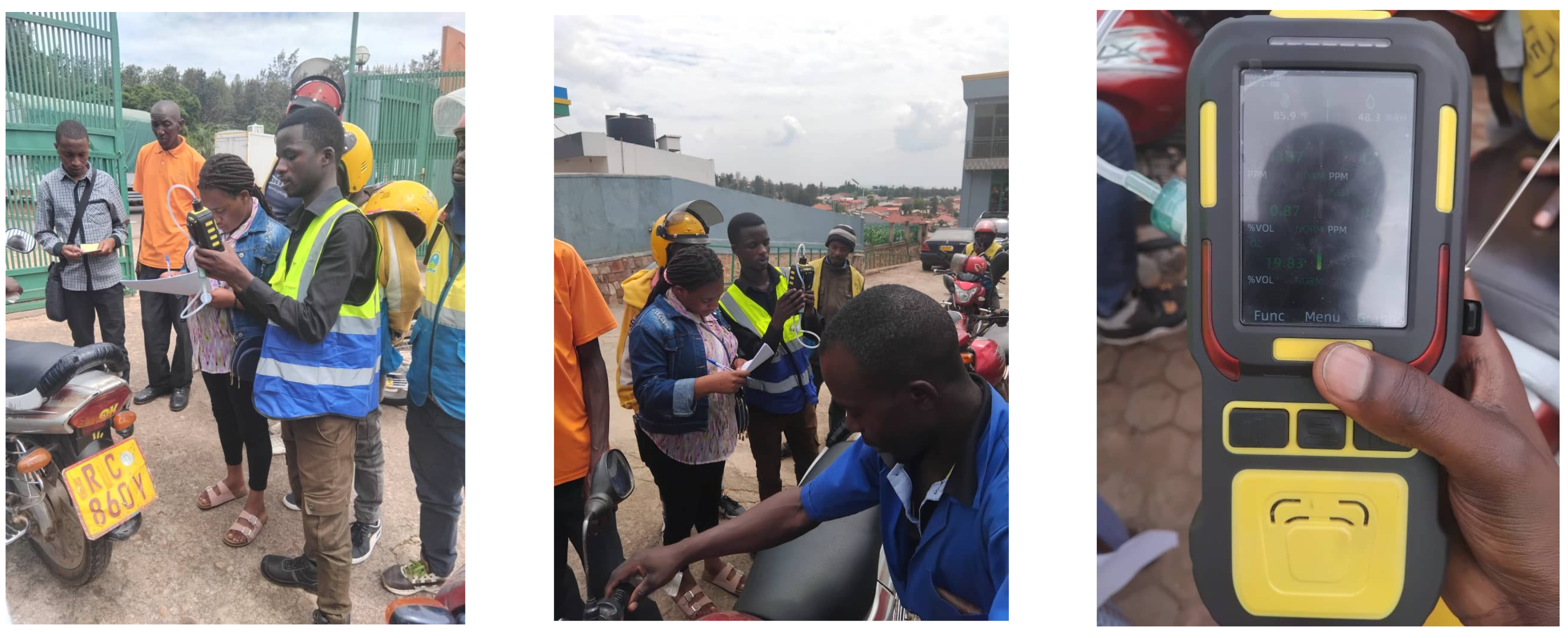
Sampling procedure: Within each stratum (a unique combination of engine capacity, year, and zone), motorcycles were selected using a simple random sampling method from official registration lists or on-site rosters at motorcycle taxi parks. This ensured that every motorcycle within a stratum had an equal probability of being selected, minimizing selection bias. Data collection: For each selected motorcycle, emissions were measured using a calibrated portable emissions monitoring system (PEMS), which recorded concentrations of CO, CO2, HC, and NO2. Each motorcycle was tested under three standardized operational conditions corresponding to controlled accelerations in first, second, and third gears. Specifically, “medium acceleration” was standardized as an increase in engine speed from 1500 to 4000 rpm (approximately 10–40 km/h in first gear, 20–60 km/h in second gear, and 30–80 km/h in third gear) maintained for a duration of 8–10 s per run. Emissions were measured using Forensics Detectors FD-600M 5-gas analyzer [33], configured for motorcycle exhaust with the following detection limits: HC (CH4) 0–10,000 ppm (1 ppm res.), CO 0–20,000 ppm (1 ppm), CO2 0–20%vol (0.01%), and NOx (NO) 0–5000 ppm (1 ppm). Daily zero/span calibration was performed per manufacturer protocol. These parameters were chosen to represent typical in-traffic acceleration patterns of urban motorcycle operation. Emissions testing followed a standardized stationary protocol [34]: measurements were captured during mid-acceleration in 1st gear, then 2nd gear, then the highest gear (8–10 s per phase, ~1500–4000 rpm), with motorcycles supported on stands. This simulates typical urban acceleration patterns while ensuring safety and consistency. Concurrently, structured interviews were conducted using a validated questionnaire to gather data on maintenance practices, daily usage, rider demographics, and socioeconomic aspects. Figure 2 presents photographs from the fieldwork, illustrating the emissions testing and interview processes.

2.2. Data Source and Preprocessing

We used emission test records from individual motorcycles, comprising averaged measurements of four key pollutants—carbon monoxide (CO), carbon dioxide (CO2), hydrocarbons (HC), and nitrogen dioxide (NO2)—alongside various associated socioeconomic and environmental attributes. However, dioxygen (O2) was measured as a combustion and reference parameter, not as an emission pollutant. Each record represents a unique motorcycle plate number and includes data on technical specifications, driver behavior, usage patterns, and operational or socioeconomic context.

Data Cleaning and Transformation

Prior to analysis, the emission dataset underwent essential preprocessing using standard data cleaning and transformation techniques. This included data normalization, handling of missing values, data type conversion, feature engineering, and dataset merging to ensure consistency, completeness, and readiness for statistical modeling [35]. Predictor variables were organized into the following three thematic groups: motorcycle characteristics, driver behavior, and usage profile, as well as socioeconomic/operational context (Table 1).

2.3. Descriptive and Exploratory Statistical Analysis of Variables Used

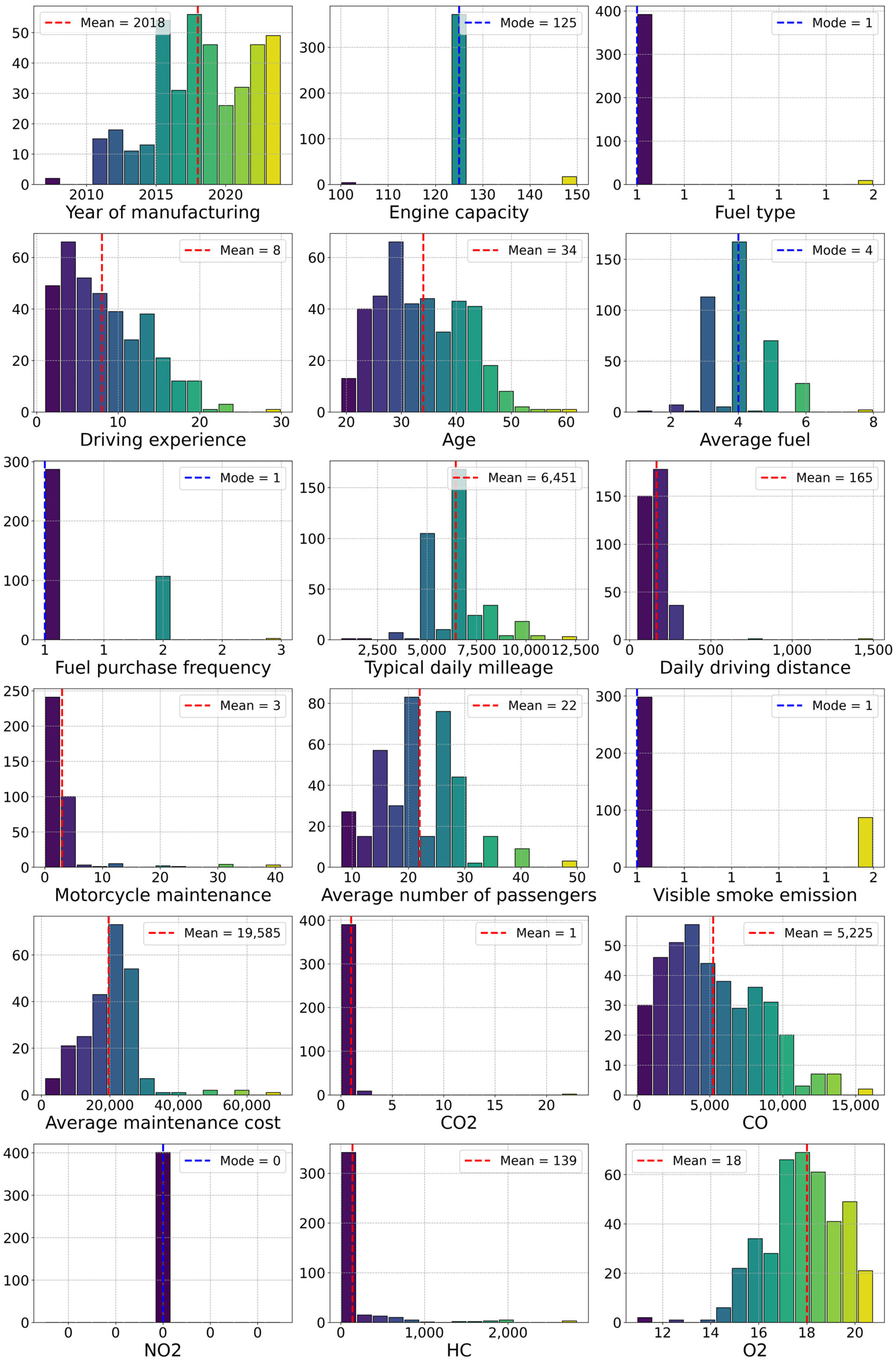
We computed descriptive statistics to summarize and explore the dataset. We describe continuous variables using measures of central tendency and dispersion (mean, standard deviation, minimum, and maximum), while categorical variables were summarized using frequencies and proportions. This step facilitated a high-level understanding of variable distributions and potential anomalies. Histograms in Figure 3 show all variables used.

2.4. The MANOVA and Kruskal–Wallis H Test Models

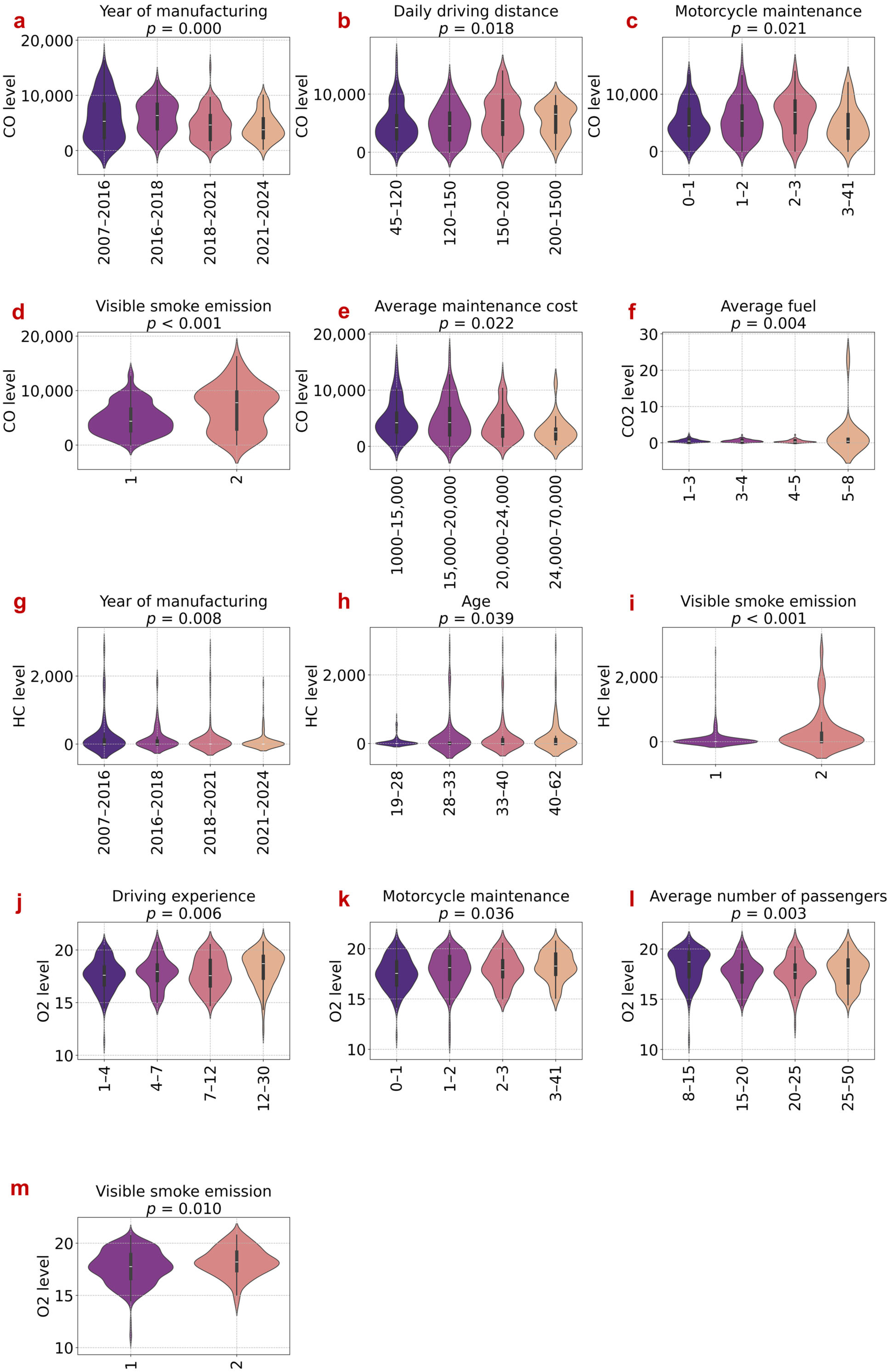
To examine the relationships between motorcycle-related features and emission levels (HC, CO, CO2, and O2), we employed a multi-method statistical approach to ensure both robustness and validity. We first transformed continuous variables into categorical groups [43], dividing each variable into four bins with approximately equal numbers of observations [44], using quantile-based binning [45]. This ensured balanced group sizes for the Kruskal–Wallis H test while preserving the ordinal nature of the data [46]. Then, we conducted MANOVA to assess the overall effect of each categorical or ordinal predictor on the combined set of emissions, under the assumptions of multivariate normality and homogeneity of variances [47,48]. Wilks’ lambda ranges from 0 to 1, where lower values indicate stronger multivariate separation among groups [48]. In this study, a smaller lambda value reflects a stronger joint influence of the predictor on the combined emission outcomes (CO, CO2, HC, and O2), whereas values closer to 1 indicate weaker or negligible multivariate effects. We used the F-statistic and corresponding p-values as evaluation criteria to assess its significance [48]. A larger F-value indicates that the group means are more distinct relative to the within-group variability, suggesting a stronger effect of the predictor on the outcome [47]. A statistically significant F-value (typically p < 0.05) implies that the predictor variable is associated with meaningful differences in emission levels, indicating its potential relevance in explaining pollutant variation [48]. Later, we applied the Shapiro–Wilk test to the residuals of the MANOVA model to assess the multivariate normality assumption [49]. At a significance level of α = 0.05, a p-value greater than α indicates that the assumption is met, whereas a p-value less than or equal to α suggests a violation of the normality assumption [50]. The results indicate that the normality assumption was met only for CO emissions (p > 0.05), while residuals for CO2, HC, and O2 significantly deviated from normality (p < 0.001). Consequently, we afterward applied the non-parametric Kruskal–Wallis H test to robustly validate and complement the MANOVA findings under violated assumptions. While MANOVA provided a holistic multivariate perspective across all emissions simultaneously, the Kruskal–Wallis H test allowed detailed investigation of feature-specific differences for each emission in a distribution-free manner. We used the Kruskal–Wallis H test results to compute the violin plots to depict the distribution of key emission metrics (CO, CO2, HC, O2) across only significant categorical group features. Finally, to capture potential nonlinear or monotonic associations that may not be detected through parametric or group comparison methods, we conducted Spearman correlation analysis [48]. This approach evaluated pairwise associations between motorcycle features and emission variables, providing insight into consistent trends and directional effects, especially for variables with skewed distributions or ordinal measurements [51]. We visualized the results using a heatmap plot, which facilitated the interpretation of positive and negative associations.

3. Results and Discussion

3.1. Descriptive Statistical Analysis and Exploratory Analysis of Variables Used

Table S1 and Figure 3 present descriptive statistics for the study variables after outlier removal. The motorcycles were relatively recent (M = 2018.3, SD = 3.56), with standardized engine capacities (M = 125.8 cc, SD = 5.7). Riders had an average age of 33.6 years (SD = 7.8) and 8.3 years of driving experience (SD = 5.3). Fuel consumption (M = 4.0 L/day, SD = 1.0) and purchase frequency (mostly once per week) were consistent across the sample. Daily usage patterns showed high variability, with average daily driving distances of 164.9 km (SD = 92.0) and typical cumulative mileage averaging 6450.6 m (SD = 1514.9). Motorcycle maintenance and visible smoke emission were recorded on ordinal scales. Many motorcycles showed low levels of visible smoke emission (M = 1), and maintenance practices varied with a long right tail (max = 41, SD = 5.2), suggesting some motorcycles are serviced unusually frequently. Emission levels varied substantially: CO2 concentrations were generally low (M = 0.63 ppm, SD = 1.64), while CO emissions were markedly high and dispersed (M = 5225 ppm, SD = 3260; max = 16,220 ppm). HC emissions were right-skewed (M = 139 ppm; median = 0), with a few motorcycles emitting extreme values (max = 2830 ppm). O2 concentrations in exhaust were within expected ranges (M = 17.8%, SD = 1.55). Relatively high O2 concentrations likely indicate lean air-fuel mixtures during controlled accelerations rather than idling or deceleration phases. NO2 values were uniformly zero and excluded from further analysis. Overall, the data reflect a largely uniform fleet with localized emission issues likely linked to maintenance practices and combustion efficiency.

3.2. The MANOVA and Kruskal–Wallis H Test Results

MANOVA was conducted to examine whether motorcycle emissions (CO, CO2, HC, and O2) differed jointly across categories of various predictor variables. Wilks’ lambda was used as the test statistic to assess multivariate group differences. The results in Table S2 indicate that several predictors showed statistically significant multivariate effects on the combined emission profile.
The MANOVA model evaluated the joint effect of each predictor on the combined emission outcomes (CO, CO2, HC, and O2). Visible smoke emission emerged as the strongest multivariate predictor, yielding a Wilks’ lambda of 0.842 (F (4, 380) = 17.77, p < 0.001), indicating a significant collective impact on emission levels. Year of manufacturing (lambda = 0.910, F = 3.14, p < 0.001), average fuel consumption (lambda = 0.915, F = 2.92, p = 0.001), and daily driving distance (lambda = 0.911, F = 2.83, p = 0.001) were also significant predictors, suggesting that newer, more fuel-efficient motorcycles with different usage patterns exhibit distinguishable emission profiles. Additionally, rider-related factors such as age (lambda = 0.937, F = 2.14, p = 0.013), average number of passengers (lambda = 0.935, F = 2.10, p = 0.015), and driving experience (lambda = 0.936, F = 2.00, p = 0.021) showed modest but significant multivariate effects. Motorcycle maintenance also reached significance (lambda = 0.938, F = 1.89, p = 0.032), indicating its role in modulating emissions across pollutants. In contrast, average maintenance cost, fuel purchase frequency, typical daily mileage, and engine capacity did not show significant multivariate associations (all p > 0.26), suggesting limited explanatory power when considering the emissions jointly.
The Kruskal–Wallis H test was conducted to assess whether different motorcycle-related features have statistically significant effects on various emissions (HC, CO, CO2, and O2). The violin results in Figure 4 highlight several features, with statistically significant group differences identified by the Kruskal–Wallis H test p-values. For example, the year of manufacturing features on both CO and HC emissions are notably lowest in the newest motorcycle group (2018–2021), intermediate among motorcycles from 2016 to 2018 and 2021–2024, and highest in the oldest group (2007–2016), suggesting effective regulatory improvements on reducing emissions (Figure 4a,g). The motorcycle maintenance feature is another critical factor; motorcycles in the poorest maintenance group (2–3) display the highest CO and O2 emissions, while better-maintained groups (especially 0–1 and 1–2) exhibit notably lower emissions, underscoring the emissions mitigation achieved through regular maintenance (Figure 4c,k). Across all pollutant types (Figure 4d,i,m), visible smoke emission functions as a powerful discriminant: motorcycles with visible smoke (2) exhibited markedly higher CO and HC emissions, alongside lower O2 emissions, compared to those without visible smoke (1), reinforcing visual exhaust inspection as a practical diagnostic for incompletely combusting or malfunctioning engines.
For daily driving distance (Figure 4b), motorcycles in the highest group (200–1500 km) exhibited elevated CO emissions relative to those in the lower distance groups (45–120 km and 150–200 km), indicating that high operational mileage accelerates engine wear or inefficiency. Looking at the average maintenance cost feature in Figure 4c,k, the highest expenditure group (24,000–70,000 RWF) was associated with the lowest CO emissions, while the lowest cost group (1000–15,000 RWF) tended toward higher emission levels, suggesting that greater investment in maintenance may correlate with cleaner operation. The average fuel consumption in Figure 4f was most tightly linked to CO2: motorcycles consuming 5–8 L/100 km produced significantly higher CO2 emissions compared to groups consuming less fuel (1–3, 3–4, and 4–5 L/100 km), highlighting direct benefits of using retrofitted motorcycles for greenhouse gas mitigation. Considering the rider age in Figure 4h, analysis revealed that younger riders (19–28 years) are associated with the highest HC emissions, whereas older riders (40–62 years) are at the lowest end, which may reflect differences in riding style or vehicle care. Similarly, in Figure 4j, riders with greater driving experience (7–12 years and 12–30 years) showed heightened O2 emission relative to the least-experienced group (1–4 years), hinting at either more efficient combustion or possible differences in riding patterns. Lastly, referring to Figure 4l, motorcycles carrying more passengers on average (25–50) also had elevated O2 emissions compared to those with fewer passengers (8–15), possibly due to increased engine load altering combustion processes.

3.3. Comparative Models Findings: MANOVA and Kruskal–Wallis H Tests

We later compared MANOVA and Kruskal–Wallis H test results to gain insight regarding the influence of various motorcycle-related features on emission levels (HC, CO, CO2, and O2). The MANOVA, based on Wilks’ lambda, evaluates differences across multiple dependent variables under assumptions of normality and homogeneity of variances, whereas the Kruskal–Wallis H test offers a distribution-free alternative, evaluating group differences for each emission type individually. Results from both methods in Figure 5 showed that visible smoke emission emerged as the strongest predictor across both analyses. It yielded the most significant multivariate effect in MANOVA (Wilks’ lambda = 0.842, F = 17.77, p < 0.001) and was highly significant across individual pollutants in the Kruskal–Wallis H test (e.g., HC: H = 30.62, p < 0.001), confirming that visually detectable emissions are strongly associated with elevated pollutant levels. The year of manufacturing feature also showed consistent results across methods, with a significant multivariate effect (Wilks’ lambda = 0.910, p < 0.001) and strong effects in the Kruskal–Wallis H test for CO (H = 20.61, p < 0.001) and HC (H = 11.80, p = 0.008). This consistency supports the interpretation that emissions vary systematically with motorcycle age, likely due to regulatory, technological, or mechanical factors. Average fuel consumption was significant in both models (MANOVA: Wilks’ lambda = 0.915, p < 0.001; Kruskal–Wallis for CO2: H = 13.32, p = 0.004), indicating a consistent relationship between fuel usage and carbon dioxide emissions. Similarly, daily driving distance, motorcycle age, passenger load, driving experience, and maintenance practices all showed statistically significant effects in both analyses, though the magnitude and the specific emission types affected varied slightly. For instance, driving experience was significant in MANOVA (p = 0.021) and showed a strong univariate effect on O2 in the Kruskal–Wallis H test (H = 12.54, p = 0.006), reflecting consistent insights across parametric and non-parametric approaches. However, we observed some divergence between models. For example, average maintenance cost was not significant in MANOVA (p = 0.268) but showed significance in the Kruskal–Wallis test for CO (H = 9.61, p = 0.022), suggesting potential nonlinear or skewed relationships that the parametric model may not fully capture. Similarly, engine capacity, fuel purchase frequency, and typical daily mileage were non-significant in both tests, indicating these features are unlikely to be strong determinants of emissions regardless of analytical method.

3.4. Bivariate Relationships Between Emissions and Predictors

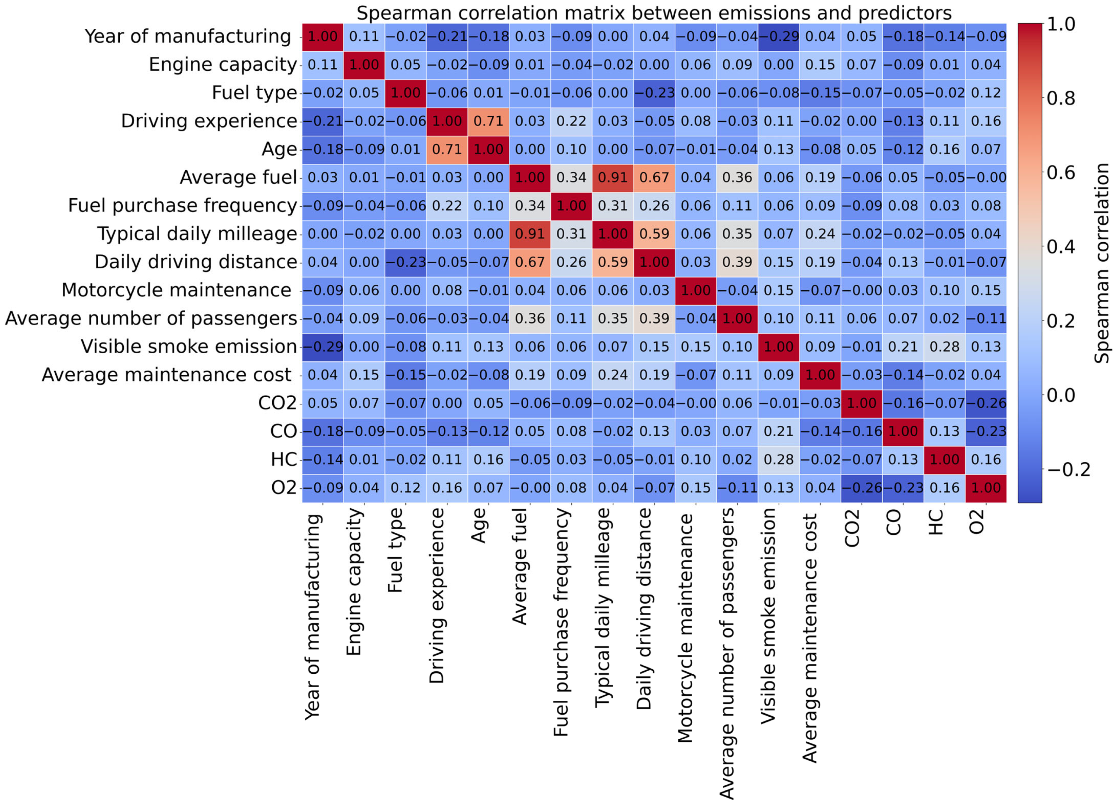
The Spearman correlation analyses in Figure 6 reveal distinct relationships between predictor variables and emission levels, emphasizing the multifaceted nature of motorcycle pollution. CO emissions are moderately and positively associated with visible smoke emission (ρ = 0.21) and negatively correlated with year of manufacturing (ρ = −0.18) and rider age (ρ = −0.12), indicating that newer motorcycles and older riders may contribute to lower CO levels, potentially due to better technology or more cautious driving behavior. HC emissions also show a notable positive correlation with visible smoke (ρ = 0.28), as well as weak-to-moderate associations with rider-related factors such as age (ρ = 0.16) and driving experience (ρ = 0.11), reinforcing the role of incomplete combustion in older or poorly maintained engines. In contrast, CO2 emissions appear largely uncorrelated with most predictors, with the highest (yet weak) correlation observed for engine capacity (ρ = 0.07). Notably, visible smoke emission is virtually uncorrelated with CO2 (ρ = −0.01), supporting the view that CO2 results from complete combustion, unlike other pollutants tied to inefficiencies. O2 levels in the exhaust correlate positively with driving experience (ρ = 0.16), motorcycle maintenance (ρ = 0.15), and visible smoke emission (ρ = 0.13), suggesting complex air-fuel dynamics and potential under- or over-combustion patterns in less efficient or more frequently serviced vehicles. Additionally, fuel-related behaviors such as average fuel consumption and fuel purchase frequency show little to no strong correlation with emissions, although average fuel is weakly related to some usage indicators (e.g., daily mileage). Overall, HC and CO emissions are more responsive to visible smoke and rider-related characteristics, while CO2 and O2 levels reflect broader aspects of combustion efficiency and engine operation.
This study elucidates the effects of a range of motorcycle-related and rider factors on key emission outputs, using both parametric and non-parametric statistical analysis. Specifically, this study leverages MANOVA’s strength of uncovering joint effects across pollutants, while the Kruskal–Wallis H test clarifies specific pollutant relationships, and Spearman correlation analysis uncovers nonlinear associations among pollutants and their predictors. Together, these approaches guide both scientific understanding and policy development toward effective emission reduction strategies. The combined use of parametric (MANOVA) and non-parametric (Kruskal–Wallis H test) provides a comprehensive understanding of how different factors influence motorcycle emissions [52]. MANOVA results are particularly valuable for identifying predictors that affect the overall emission profile [27], capturing effects that may be distributed across multiple pollutants and potentially missed by individual Kruskal–Wallis H tests [48]. This is evident for predictors like daily driving distance and age, which show significance only in the multivariate context (Figure 2). Conversely, the Kruskal–Wallis H test results are essential for pinpointing which specific pollutants are most affected by each predictor. For example, average fuel and motorcycle maintenance show their strongest effects on CO and CO2, suggesting that targeted interventions could focus on these emissions for those factors [53]. The clear and consistent significance of visible smoke emission across both analyses supports its use as a practical field diagnostic and a scientifically robust marker for high emissions [54]. This finding aligns with studies in other contexts that have recommended visible smoke checks as a cost-effective screening tool for vehicle emissions [37,55]. These results highlight the importance of using parametric and non-parametric multivariate approaches when analyzing environmental data with multiple, correlated outcomes [56]. MANOVA can reveal joint effects that univariate Kruskal–Wallis H test methods may overlook [57], while the Kruskal–Wallis H test clarifies the contribution of each predictor to individual pollutants [58]. This dual approach is supported by statistical best practices and is increasingly recommended in environmental health research [48]. Similar studies have reported comparable findings. For instance, [59] demonstrated that visible smoke and maintenance practices were strong predictors of motorcycle emissions in urban China, while [52] and [27] emphasized the value of multivariate techniques in environmental monitoring for capturing complex, multi-pollutant effects. Although engine capacity is theoretically linked to higher combustion and emissions [37,60,61], the motorcycles in our sample showed only a very narrow range of engine sizes (100–150 cc). This limited variation reduces the ability to detect statistical differences. In this fleet, stronger predictors such as year of manufacture, visible smoke, and maintenance condition had much larger effects, which likely overshadowed the small influence of engine capacity. In this study, observed zero NO2 values are likely due to the detection limits and configuration of the portable emissions monitoring system (FD-600M) used, optimized for real-time measurement of CO, CO2, HC, and O2 during short acceleration tests. Under these controlled conditions (8–10 s per gear), NO2 concentrations likely fell below the analyzer’s reporting threshold. Other studies using chemiluminescence analyzers or longer driving tests have found substantial NOx emissions from motorcycles [62,63]. Therefore, the zero values here reflect measurement limitations rather than the absence of NOx emissions.
The Spearman correlation findings highlight the complex interplay between motorcycle emissions and various technical and behavioral factors. The observed moderate positive association between CO and visible smoke emissions, alongside negative correlations with motorcycle age and rider age, aligns with previous research indicating that older vehicles and less experienced or younger riders tend to contribute more to urban air pollution due to outdated technology and riskier driving behaviors [64,65]. The positive relationship between HC emissions and both visible smoke and rider-related factors further supports the notion that incomplete combustion, often stemming from poor maintenance or older engines, remains a key driver of hydrocarbon pollution [66]. Interestingly, the weak correlations between CO2 emissions and most predictors, notably the near-zero association with visible smoke, reinforce the understanding that CO2 is a product of complete combustion, distinguishing it from pollutants like CO and HC that are more sensitive to inefficiencies and operational habits [67]. The positive links between O2 levels and factors such as driving experience and maintenance suggest that frequent servicing or experienced riders may influence air fuel mixtures, potentially reflecting both improved and suboptimal combustion scenarios [24].
While this study reveals meaningful associations between vehicle/rider characteristics and emissions, several limitations must be acknowledged. First, the cross-sectional nature of the analysis restricts causal inference [68], and the reliance on self-reported rider characteristics may introduce bias [69]. Additionally, this study did not account for emissions during engine idling, acceleration or deceleration phases, or hill climbs with passenger loads under conditions typical of urban motorcycle use in the city of Kigali. As a result, the emission measurements may not fully reflect real-world operating conditions, potentially affecting the accuracy of estimated pollutant levels. Future research should incorporate more representative drive cycles to improve realism and comparability [55]. Second, MANOVA also has an interpretability challenge. While a significant MANOVA result confirms that group differences exist in the multivariate outcome space, it does not specify which dependent variables are driving the effect [70]. This necessitates the Kruskal–Wallis H test or other statistical approaches, including discriminant analyses, to identify the specific pollutants involved [48]. Additionally, MANOVA assumes multivariate normality and homogeneity of variance [70], conditions that may not always hold in real-world environmental data [71]. Violations of these assumptions can affect the robustness of the results [72]. Furthermore, our analyses were constrained by substantial non-response, which reduced statistical power and may have biased weaker associations toward the null. Accordingly, results derived from predictors with markedly lower sample sizes should be interpreted with particular caution. Given these strengths and limitations, future research should consider several directions. First, incorporating larger and more diverse datasets could improve the generalizability of findings and allow for more sophisticated modeling, such as mixed-effects MANOVA [73] or structural equation modeling [9,74], which can handle hierarchical data and latent variables [72]. Second, integrating additional predictors such as fuel type, maintenance history, and environmental conditions may help disentangle the complex drivers of emissions [42]. Third, further studies could employ post hoc analyses or machine learning approaches to better interpret which combinations of pollutants and predictors are most critical for targeted interventions [75]. Future work should also prioritize experimental validation through controlled emissions testing [76], longitudinal monitoring of vehicle aging effects [77], and machine learning approaches incorporating granular predictors like ambient temperature and real-world driving cycles [78]. Such advancements would strengthen emission mitigation strategies, particularly for high HC-emitting older motorcycles [17]. The NOx concentration was measured using the FD-600M analyzer with an NO2 detection limit of 0.1 ppm in a 0–20 ppm range. The observed zero values likely result from concentrations falling below this detection threshold during short test conditions or limitations in analyzer sensitivity rather than the true absence of NO2 emissions. Therefore, uniformly zero NO2 readings reflect measurement limitations and do not indicate negligible NOx emissions in the fleet.

4. Conclusions and Recommendations

This study investigates the influence of various motorcycle-related factors on emissions through a comparative analysis employing multivariate MANOVA, Kruskal–Wallis H test, and Spearman correlation methods. Visible smoke consistently emerged as the strongest predictor in both analyses, underscoring its practical and scientific value as a low-cost diagnostic tool. While MANOVAs captured broader joint effects that individual tests could overlook, Kruskal–Wallis H tests clarified which pollutants were most affected by each variable, particularly for predictors such as year of manufacturing, and additionally highlighted motorcycle maintenance as a key factor influencing emission differences. Spearman correlation results further supported these trends, revealing strong positive associations between visible smoke and both CO and HC, along with notable behavioral effects tied to rider age and experience. Together, these findings highlight the importance of integrating mixed multivariate and pollutant-specific methods to guide policy, inspection protocols, and targeted interventions aimed at reducing motorcycle emissions in resource-constrained settings. This study demonstrated that older and poorly maintained vehicles emit higher CO and HC, while larger engine capacities and irregular servicing increase CO2 and NO2. Well-maintained motorcycles showed lower emissions, highlighting the importance of maintenance and engine condition in pollution control. The authors recommend the following: (1) implementing a mandatory fail criterion for visible smoke in roadside inspections and annual fitness tests; (2) targeting motorcycles manufactured before 2016 for retrofitting or scrappage; and (3) developing rider training programs to mitigate high HC emissions among younger, less experienced operators. This study presents the first hybrid multivariate and non-parametric analysis of African moto-taxi emissions, identifying visible smoke as the optimal low-cost screening proxy, highlighting the importance of pre-2018 fleet maintenance, and demonstrating robust approaches for skewed emission data in data-scarce contexts. Combined with systematic emission monitoring and strengthened maintenance enforcement, these measures offer a practical, evidence-based approach to cleaner motorcycle fleets and improved urban air quality.

Supplementary Materials

The following supporting information can be downloaded at: https://www.mdpi.com/article/10.3390/atmos17010047/s1. Table S1. Descriptive statistics of variables used in the analysis; Table S2. MANOVA results for motorcycle features.

Author Contributions

G.G.A.: conceptualization, supervision, project administration, writing the original draft, and validation; B.B.M.: conceptualization, supervision, project administration, critical review, editing, and validation; H.B., J.N., M.N., J.d.D.M., D.R.K., M.M., T.H., E.T., T.M. and P.B.B.: supervision, critical review, editing, and validation; G.N.: conceptualization, data curation, methodology, writing the original draft, critical review, editing, and validation. All authors have read and agreed to the published version of the manuscript.

Funding

This research was financially supported by the National Council for Science and Technology (NCST), Rwanda, under the Research and Innovation Grant No. NCST-NRIF/RIC-R&D–PHASE I/08/10/2022. The authors gratefully acknowledge this support, which made the successful completion of this study possible.

Institutional Review Board Statement

Not applicable.

Informed Consent Statement

Not applicable.

Data Availability Statement

The datasets and Python 3.14.2 codes used in this study are available from the corresponding author upon reasonable request.

Conflicts of Interest

Authors Donald Rukotana Kabanda, Maximillien Mutuyeyezu and Prince Bonfils Bimenyimana were employed by the company Rwanda Electric Mobility (REM Ltd.). Author Emmanuel Tuyizere was employed by the company Greenalytic Motors Ltd. The remaining authors declare that the research was conducted in the absence of any commercial or financial relationships that could be construed as a potential conflict of interest.

References

  1. Amegah, A.K.; Agyei-Mensah, S. Urban Air Pollution in Sub-Saharan Africa: Time for Action. Environ. Pollut. 2017, 220, 738–743. [Google Scholar] [CrossRef] [PubMed]
  2. Pochet, P.; Lesteven, G. The Spread of Motorcycles in Sub-Saharan Africa: Dynamics and Public Issues. Transp. Res. Procedia 2025, 82, 3237–3250. [Google Scholar] [CrossRef]
  3. Ehebrecht, D.; Heinrichs, D.; Lenz, B. Motorcycle-Taxis in Sub-Saharan Africa: Current Knowledge, Implications for the Debate on “Informal” Transport and Research Needs. J. Transp. Geogr. 2018, 69, 242–256. [Google Scholar] [CrossRef]
  4. Diaz Olvera, L.; Plat, D.; Pochet, P. Looking for the Obvious: Motorcycle Taxi Services in Sub-Saharan African Cities. J. Transp. Geogr. 2020, 88, 102476. [Google Scholar] [CrossRef]
  5. Alimo, P.K.; Lartey-Young, G.; Agyeman, S.; Akintunde, T.Y.; Kyere-Gyeabour, E.; Krampah, F.; Awomuti, A.; Oderinde, O.; Agbeja, A.O.; Afolabi, O.G. Spatial Distribution and Policy Implications of the Exhaust Emissions of Two-Stroke Motorcycle Taxis: A Case Study of Southwestern State in Nigeria. J. Niger. Soc. Phys. Sci. 2024, 6, 1898. [Google Scholar] [CrossRef]
  6. Vanatta, M.; Rathod, B.; Calzavara, J.; Courtright, T.; Sims, T.; Saint-Sernin, É.; Clack, H.; Jagger, P.; Craig, M. Emissions Impacts of Electrifying Motorcycle Taxis in Kampala, Uganda. Transp. Res. Part Transp. Environ. 2022, 104, 103193. [Google Scholar] [CrossRef]
  7. Adiang, C.M.; Monkam, D.; Njeugna, E.; Gokhale, S. Projecting Impacts of Two-Wheelers on Urban Air Quality of Douala, Cameroon. Transp. Res. Part Transp. Environ. 2017, 52, 49–63. [Google Scholar] [CrossRef]
  8. Courtright, T.; Behrens, R. The Role and Impact of Motorcycle-Taxis: A Systematic Review. Transp. Res. Procedia 2025, 89, 104–116. [Google Scholar] [CrossRef]
  9. Nguyen-Phuoc, D.Q.; Truong, T.M.; Nguyen, M.H.; Pham, H.G.; Li, Z.C.; Oviedo-Trespalacios, O. What Factors Influence the Intention to Use Electric Motorcycles in Motorcycle-Dominated Countries? An Empirical Study in Vietnam. Transp. Policy 2024, 146, 193–204. [Google Scholar] [CrossRef]
  10. Vasic, A.M.; Weilenmann, M. Comparison of Real-World Emissions from Two-Wheelers and Passenger Cars. Environ. Sci. Technol. 2006, 40, 149–154. [Google Scholar] [CrossRef] [PubMed]
  11. Elisephane, I.; Zoltán, T. Environmental determinants of ambient air pollution in Urban East Africa: Unveiling critical insights from Kigali, Rwanda. Sci. Afr. 2025, 30, e03055. [Google Scholar] [CrossRef]
  12. Ehebrecht, D. Motorcycle-Taxis in East African Cities: Growth Dynamics, Regulation, Challenges and Potentials. In Transport Planning and Mobility in Urban East Africa; Routledge: London, UK, 2020; pp. 136–160. [Google Scholar] [CrossRef]
  13. Alimo, P.K.; Rahim, A.B.A.; Lartey-Young, G.; Ehebrecht, D.; Wang, L.; Ma, W. Investigating the Increasing Demand and Formal Regulation of Motorcycle Taxis in Ghana. J. Transp. Geogr. 2022, 103, 103398. [Google Scholar] [CrossRef]
  14. Diaz Olvera, L.; Guézéré, A.; Plat, D.; Pochet, P. Earning a Living, but at What Price? Being a Motorcycle Taxi Driver in a Sub-Saharan African City. J. Transp. Geogr. 2016, 55, 165–174. [Google Scholar] [CrossRef]
  15. Owino, F.; Peters, K.; Jenkins, J.; Opiyo, P.; Chetto, R.; Ntramah, S.; Marion Mutabazi, M.; Vincent, J.; Johnson, T.P.; Santos, R.T.; et al. The Urban Motorcycle Taxi Sector in Sub-Saharan Africa: Needs, Practices and Equity Issues. Urban Plan. Transp. Res. 2024, 12, 2354400. [Google Scholar] [CrossRef]
  16. Martin, E.; Courtright, T.; Nkurunziza, A.; Lah, O. Motorcycle Taxis in Transition? Review of Digitalization and Electrification Trends in Selected East African Capital Cities. Case Stud. Transp. Policy 2023, 13, 101057. [Google Scholar] [CrossRef]
  17. Koossalapeerom, T.; Satiennam, T.; Satiennam, W.; Leelapatra, W.; Seedam, A.; Rakpukdee, T. Comparative Study of Real-World Driving Cycles, Energy Consumption, and CO2 Emissions of Electric and Gasoline Motorcycles Driving in a Congested Urban Corridor. Sustain. Cities Soc. 2019, 45, 619–627. [Google Scholar] [CrossRef]
  18. Health Effects Institute. Traffic-Related Air Pollution: A Critical Review of the Literature on Emissions, Exposure, and Health Effects | Health Effects Institute. 2010. Available online: https://www.healtheffects.org/publication/traffic-related-air-pollution-critical-review-literature-emissions-exposure-and-health (accessed on 26 August 2025).
  19. Sudmant, A.; Colenbrander, S.; Gouldson, A.; Chilundika, N. Private Opportunities, Public Benefits? The Scope for Private Finance to Deliver Low-Carbon Transport Systems in Kigali, Rwanda. Urban Clim. 2017, 20, 59–74. [Google Scholar] [CrossRef]
  20. Colenbrander, S.; Sudmant, A.; Chilundika, N.; Gouldson, A. The Scope for Low-Carbon Development in Kigali, Rwanda: An Economic Appraisal. Sustain. Dev. 2019, 27, 349–365. [Google Scholar] [CrossRef]
  21. Marija, J.; Amponsah, O.; Mensah, H.; Takyi, A.; Braimah, I. A View of Commercial Motorcycle Transportation in Sub-Saharan African Cities Through the Sustainable Development Lens. Transp. Dev. Econ. 2022, 8, 13. [Google Scholar] [CrossRef]
  22. Irankunda, E.; Török, Z. Monitoring and Dispersion Modelling of Particulate Matter (PM2.5) in Rwanda. In Aerosol Science and Engineering; Springer: Berlin/Heidelberg, Germany, 2025; pp. 1–18. [Google Scholar] [CrossRef]
  23. Sietchiping, R.; Permezel, M.J.; Ngomsi, C. Transport and Mobility in Sub-Saharan African Cities: An Overview of Practices, Lessons and Options for Improvements. Cities 2012, 29, 183–189. [Google Scholar] [CrossRef]
  24. Ghaffarpasand, O.; Talaie, M.R.; Ahmadikia, H.; Khozani, A.T.; Shalamzari, M.D.; Majidi, S. Real-World Evaluation of Driving Behaviour and Emission Performance of Motorcycle Transportation in Developing Countries: A Case Study of Isfahan, Iran. Urban Clim. 2021, 39, 100923. [Google Scholar] [CrossRef]
  25. Filonchyk, M.; Peterson, M.P. Analysis of Air Pollution from Vehicle Emissions for the Contiguous United States. J. Geovisualization Spat. Anal. 2024, 8, 16. [Google Scholar] [CrossRef]
  26. Singh, S.; Kulshrestha, M.J.; Rani, N.; Kumar, K.; Sharma, C.; Aswal, D.K. An Overview of Vehicular Emission Standards. Mapan-J. Metrol. Soc. India 2023, 38, 241–263. [Google Scholar] [CrossRef]
  27. Salih, S.S.; Alkarkhi, A.F.M.; Bin Lalung, J.; Ismail, N. Water Quality of River, Lake and Drinking Water Supply in Penang State by Means of Multivariate Analysis. World Appl. Sci. J. 2013, 26, 75–82. [Google Scholar]
  28. Rencher, A.C.; Christensen, W.F. Methods of Multivariate Analysis; Wiley: Hoboken, NJ, USA, 2012; ISBN 0-470-17896-5. [Google Scholar]
  29. Okoye, K.; Hosseini, S. Mann–Whitney U Test and Kruskal–Wallis H Test Statistics in R. In R Programming: Statistical Data Analysis in Research; Springer: Singapore, 2024; pp. 225–246. [Google Scholar] [CrossRef]
  30. Zhou, Y.; Levy, J.I. Factors Influencing the Spatial Extent of Mobile Source Air Pollution Impacts: A Meta-Analysis. BMC Public Health 2007, 7, 89. [Google Scholar] [CrossRef]
  31. Nduwayezu, G.; Manirakiza, V.; Mugabe, L.; Malonza, J.M. Urban Growth and Land Use/Land Cover Changes in the Post-Genocide Period, Kigali, Rwanda. Environ. Urban. Asia 2021, 12, S127–S146. [Google Scholar] [CrossRef]
  32. Nduwayezu, G.; Kagoyire, C.; Zhao, P.; Eklund, L.; Pilesjo, P.; Bizimana, J.P.; Mansourian, A. Spatial Machine Learning for Exploring the Variability in Low Height-For-Age From Socioeconomic, Agroecological, and Climate Features in the Northern Province of Rwanda. GeoHealth 2024, 8, e2024GH001027. [Google Scholar] [CrossRef] [PubMed]
  33. FORENSICS Forensics Detectors FD-600M Gas Analyzer Installation Guide. Available online: https://manuals.plus/forensics-detectors/fd-600m-gas-analyzer-manual (accessed on 27 November 2025).
  34. United Nations/ECE. Worldwide Harmonized Motorcycle Emissions Certification Procedure (WMTC): Technical Report/: Transmitted by the Expert from Germany. 2004. Available online: https://digitallibrary.un.org/record/521702?ln=en&v=pdf (accessed on 12 August 2025).
  35. Nduwayezu, G.; Mansourian, A.; Bizimana, J.P.; Pilesjö, P. Hybridizing Spatial Machine Learning to Explore the Fine-Scale Heterogeneity between Stunting Prevalence and Its Associated Risk Determinants in Rwanda. Geo-Spat. Inf. Sci. 2025, 1–21. [Google Scholar] [CrossRef]
  36. Garcia, L.F.A.; Corrêa, S.M.; Penteado, R.; Daemme, L.C.; Gatti, L.V.; Alvim, D.S. Measurements of Emissions from Motorcycles and Modeling Its Impact on Air Quality. J. Braz. Chem. Soc. 2013, 24, 375–384. [Google Scholar] [CrossRef]
  37. Ting, Y.C.; Chang, P.K.; Hung, P.C.; Chou, C.C.K.; Chi, K.H.; Hsiao, T.C. Characterizing Emission Factors and Oxidative Potential of Motorcycle Emissions in a Real-World Tunnel Environment. Environ. Res. 2023, 234, 116601. [Google Scholar] [CrossRef]
  38. Team BikeAdvice. Types of Motorcycle Emissions and Their Effects. Available online: https://bikeadvice.in/types-emissions-effects/ (accessed on 2 May 2025).
  39. Redman, C. The Impact of Motorcycles on Air Quality and Climate Change: A Study on the Potential of Two-Wheeled Electric Vehicles. Bachelor’s Thesis, Claremont McKenna College, Claremont, CA, USA, 2015. [Google Scholar]
  40. Pinto, J.A.; Kumar, P.; Alonso, M.F.; Andreão, W.L.; Pedruzzi, R.; dos Santos, F.S.; Moreira, D.M.; Albuquerque, T.T.d.A. Traffic Data in Air Quality Modeling: A Review of Key Variables, Improvements in Results, Open Problems and Challenges in Current Research. Atmos. Pollut. Res. 2020, 11, 454–468. [Google Scholar] [CrossRef]
  41. Mahesh, S.; Ramadurai, G.; Shiva Nagendra, S.M. Real-World Emissions of Gaseous Pollutants from Motorcycles on Indian Urban Arterials. Transp. Res. Part Transp. Environ. 2019, 76, 72–84. [Google Scholar] [CrossRef]
  42. Chiou, Y.C.; Chen, T.C. Direct and Indirect Factors Affecting Emissions of Cars and Motorcycles in Taiwan. Transportmetrica 2010, 6, 215–233. [Google Scholar] [CrossRef]
  43. Nduwayezu, G.; Zhao, P.; Pilesjö, P.; Bizimana, J.P.; Mansourian, A. Multilevel Small-Area Childhood Stunting Risk Estimation: Insights from Spatial Ensemble Learning, Agro-Ecological and Environmentally Remotely Sensed Indicators. Environ. Sustain. Indic. 2025, 27, 100822. [Google Scholar] [CrossRef]
  44. Angier, D.M.; Mayer, J.D. A Comparison of Methods for Binning Responses to Open-Ended Survey Items About Everyday Events: A New Tailored-Binning Approach. Humanit. Soc. Sci. Res. 2025, 8, 32. [Google Scholar] [CrossRef]
  45. Berrettini, M.; Hennig, C.M.; Viroli, C. The Quantile-Based Classifier with Variable-Wise Parameters. Can. J. Stat. 2025, 53, e11837. [Google Scholar] [CrossRef]
  46. Boulle, M. Optimal Bin Number for Equal Frequency Discretizations in Supervized Learning. Intell. Data Anal. 2005, 9, 175–188. [Google Scholar] [CrossRef]
  47. Manly, B.F.J.; Navarro Alberto, J.A.; Gerow, K. Multivariate Statistical Methods: A Primer. In Multivariate Statistical Methods; McGraw-Hill Professional: New York, NY, USA, 2024. [Google Scholar] [CrossRef]
  48. Field, A. Discovering Statistics Using IBM SPSS Statistics; SAGE Publications Ltd.: London, UK, 2017. [Google Scholar]
  49. González-Estrada, E.; Villaseñor, J.A.; Acosta-Pech, R. Shapiro-Wilk Test for Multivariate Skew-Normality. Comput. Stat. 2022, 37, 1985–2001. [Google Scholar] [CrossRef]
  50. Villasenor Alva, J.A.; Estrada, E.G. A Generalization of Shapiro–Wilk’s Test for Multivariate Normality. Commun. Stat. Methods 2009, 38, 1870–1883. [Google Scholar] [CrossRef]
  51. MacFarland, T.W.; Yates, J.M. Introduction to Nonparametric Statistics for the Biological Sciences Using R; Springer: Berlin/Heidelberg, Germany, 2016. [Google Scholar] [CrossRef]
  52. De Almeida, F.; Correia, A.; Silva, E.C.E. Air Quality Assessment in Portugal and the Special Case of the Tâmega e Sousa Region. In Proceedings of the 1st International Conference on Applied Mathematics and Computer Science, Rome, Italy, 27–29 January 2017; p. 1836. [Google Scholar] [CrossRef]
  53. Zhou, Q.; Yun, J.; Li, X.; Zhang, X.; Liu, B.; Zhang, S.; Zheng, X.; Yue, W.; Li, X.; Zhang, W. Vehicle Emissions in a Megacity of Xi’an in China: A Comprehensive Inventory, Air Quality Impact, and Policy Recommendation. Urban Clim. 2023, 52, 101740. [Google Scholar] [CrossRef]
  54. Dhital, N.B.; Yang, H.H.; Wang, L.C.; Hsu, Y.T.; Zhang, H.Y.; Young, L.H.; Lu, J.H. VOCs Emission Characteristics in Motorcycle Exhaust with Different Emission Control Devices. Atmos. Pollut. Res. 2019, 10, 1498–1506. [Google Scholar] [CrossRef]
  55. Nguyen, Y.L.T.; Nguyen Duc, K.; Le, A.T.; Nghiem, T.D.; Than, H.Y.T. Impact of Real-World Driving Characteristics on the Actual Fuel Consumption of Motorcycles and Implications for Traffic-Related Air Pollution Control in Vietnam. Fuel 2023, 345, 128256. [Google Scholar] [CrossRef]
  56. Spector, P.E. Multivariate Data Analysis for Outcome Studies. Am. J. Community Psychol. 1981, 9, 45–53. [Google Scholar] [CrossRef]
  57. Reinhart, A.M. Multivariate Analysis of Variance (MANOVA). In The SAGE Encyclopedia of Communication Research Methods; SAGE Publications, Inc.: London, UK, 2017; pp. 1059–1062. [Google Scholar] [CrossRef]
  58. Ganesh, S. Multivariate Linear Regression. In International Encyclopedia of Education, 3rd ed.; Elsevier: Amsterdam, The Netherlands, 2009; pp. 324–331. [Google Scholar] [CrossRef]
  59. Zhang, Z.; Man, H.; Zhao, J.; Huang, W.; Huang, C.; Jing, S.; Luo, Z.; Zhao, X.; Chen, D.; He, K.; et al. VOC and IVOC Emission Features and Inventory of Motorcycles in China. J. Hazard. Mater. 2024, 469, 133928. [Google Scholar] [CrossRef]
  60. Tsai, J.H.; Chiang, H.L.; Hsu, Y.C.; Peng, B.J.; Hung, R.F. Development of a Local Real World Driving Cycle for Motorcycles for Emission Factor Measurements. Atmos. Environ. 2005, 39, 6631–6641. [Google Scholar] [CrossRef]
  61. Mulyadi, A.M.; Gunarta, S. Model of Carbon Dioxide (CO2) Emission from Motorcycle to the Manufactures, Engine Displacement, Service Life and Travel Speed. Appl. Mech. Mater. 2015, 776, 361–370. [Google Scholar] [CrossRef]
  62. Schurl, S.; Keller, S.; Lankau, M.; Hafenmayer, C.; Schmidt, S.; Kirchberger, R. RDE Methodology Development for Motorcycle Emissions Assessment. SAE Int. J. Adv. Curr. Pract. Mobil. 2025, 7, 1910–1922. [Google Scholar] [CrossRef]
  63. Radjawane, L.E. A Systematic Literature Review: Traffic Management for Motorcycles to Improve Urban Road Air Quality. Period. Polytech. Transp. Eng. 2026, 54, 105–118. [Google Scholar] [CrossRef]
  64. Leong, S.T.; Muttamara, S.; Laortanakul, P. Evaluation of Air Pollution Burden from Contribution of Motorcycle Emission in Bangkok. Water Air Soil Pollut. 2001, 131, 41–60. [Google Scholar] [CrossRef]
  65. Ng, W.S. Urban Transportation Mode Choice and Carbon Emissions in Southeast Asia. Transp. Res. Rec. 2018, 2672, 54–67. [Google Scholar] [CrossRef]
  66. Kumar Pathak, S.; Sood, V.; Singh, Y.; Channiwala, S.A. Real World Vehicle Emissions: Their Correlation with Driving Parameters. Transp. Res. Part Transp. Environ. 2016, 44, 157–176. [Google Scholar] [CrossRef]
  67. Adak, P.; Sahu, R.; Elumalai, S.P. Development of Emission Factors for Motorcycles and Shared Auto-Rickshaws Using Real-World Driving Cycle for a Typical Indian City. Sci. Total Environ. 2016, 544, 299–308. [Google Scholar] [CrossRef] [PubMed]
  68. Pearl, J. Causality: Models, Reasoning, and Inference; Cambridge University Press: New York, NY, USA, 2003; Volume 19. [Google Scholar]
  69. Khader, A.I.; Martin, R.S. On-the-Road Testing of the Effects of Driver’s Experience, Gender, Speed, and Road Grade on Car Emissions. J. Air Waste Manag. Assoc. 2019, 69, 1182–1194. [Google Scholar] [CrossRef]
  70. Finch, H.; French, B. A Monte Carlo Comparison of Robust MANOVA Test Statistics. J. Mod. Appl. Stat. Methods 2013, 12, 4. [Google Scholar] [CrossRef]
  71. Asmamaw, M.; Tiku Mereta, S.; Ambelu, A. Response of Macroinvertebrates to Changes in Stream Flow and Habitat Conditions in Dinki Watershed, Central Highlands of Ethiopia. Ecol. Indic. 2021, 133, 108448. [Google Scholar] [CrossRef]
  72. Tabachnick, B.; Fidell, L.; Ullman, J. Using Multivariate Statistics; Allyn & Bacon/Pearson Education: Boston, MA, USA, 2007; ISBN 978-0-13-479054-1. [Google Scholar]
  73. Baayen, R.H.; Davidson, D.J.; Bates, D.M. Mixed-Effects Modeling with Crossed Random Effects for Subjects and Items. J. Mem. Lang. 2008, 59, 390–412. [Google Scholar] [CrossRef]
  74. Shakya, L.K.; Devkota, N.; Dhakal, K.; Poudyal, R.; Mahato, S.; Paudel, U.R.; Parajuli, S. Consumer’s Behavioural Intention towards Adoption of e-Bike in Kathmandu Valley: Structural Equation Modelling Analysis. Environ. Dev. Sustain. 2025, 27, 16237–16265. [Google Scholar] [CrossRef]
  75. Ferreira, E.; Macedo, E.; Fernandes, P.; Coelho, M.C. A Combined Framework of Biplots and Machine Learning for Real-World Driving Volatility and Emissions Data Interpretation. Sustain. Cities Soc. 2023, 99, 104945. [Google Scholar] [CrossRef]
  76. Kroll, J.H.; Heald, C.L.; Cappa, C.D.; Farmer, D.K.; Fry, J.L.; Murphy, J.G.; Steiner, A.L. The Complex Chemical Effects of COVID-19 Shutdowns on Air Quality. Nat. Chem. 2020, 12, 777–779. [Google Scholar] [CrossRef]
  77. Baklanov, A.; Zhang, Y. Advances in Air Quality Modeling and Forecasting. Glob. Transit. 2020, 2, 261–270. [Google Scholar] [CrossRef]
  78. Smit, R.; Kingston, P.; Neale, D.W.; Brown, M.K.; Verran, B.; Nolan, T. Monitoring On-Road Air Quality and Measuring Vehicle Emissions with Remote Sensing in an Urban Area. Atmos. Environ. 2019, 218, 116978. [Google Scholar] [CrossRef]
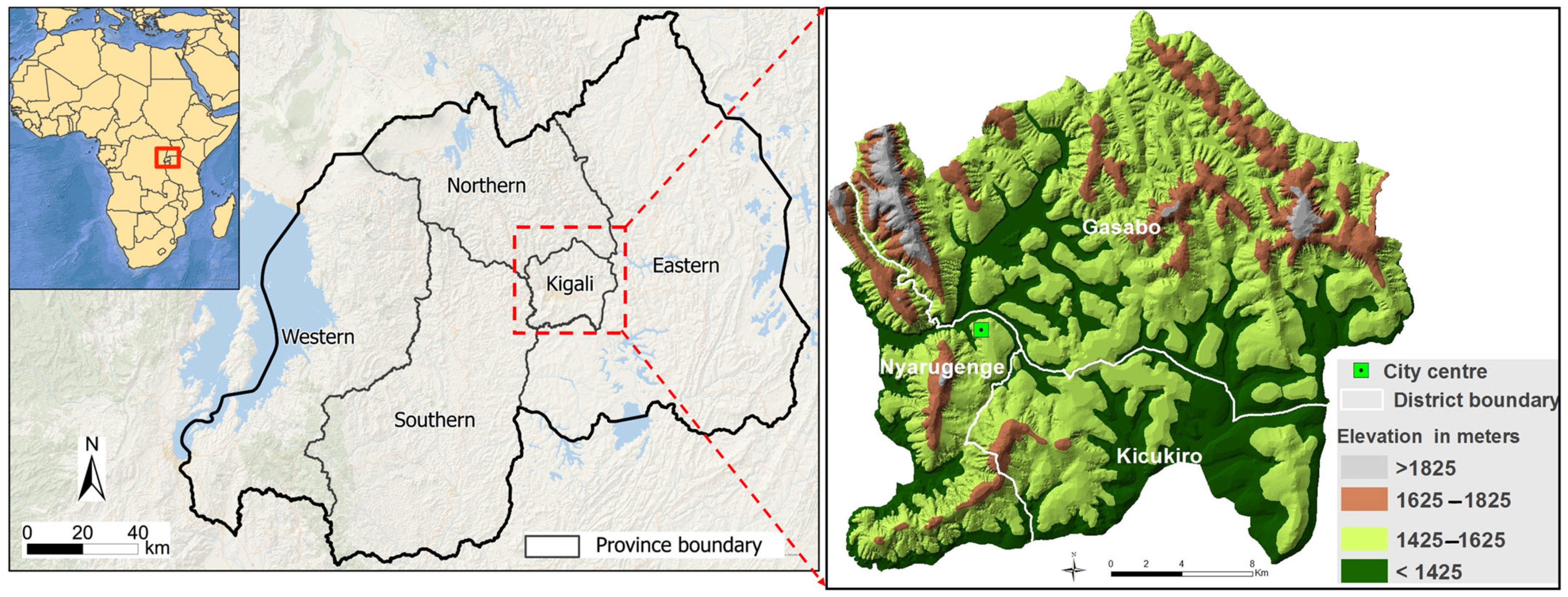
Figure 1. Location map of the city of Kigali and its districts [31].
Atmosphere 17 00047 g001
Figure 2. Emissions testing and interviews were conducted in the city of Kigali. Photos taken by the authors during fieldwork.
Atmosphere 17 00047 g002
Figure 3. Histograms showing the distributions of numeric variables in the cleaned dataset. Each panel corresponds to one variable, named below the x-axis. Histogram bins are colored by value intensity using a viridis colormap. For categorical variables, the mode is indicated by a blue dashed line; for continuous variables, the mean is indicated by a red dashed line. Corresponding values and units are provided in Table 1.
Atmosphere 17 00047 g003
Figure 4. Significant associations between motorcycle features and emission levels. Violin plots show the distributions of emission measurements (CO, CO2, HC, and O2) across quartile-binned numeric features or categorical groups; the width of each violin indicates the density of observations at each emission level, with wider sections representing higher concentrations of motorcycles at that value. Boxplots indicate medians and interquartile ranges, and colors reflect ordered categories us-ing a magma palette. Panels display only feature–emission pairs with significant Kruskal–Wallis results (italic p < 0.05). (a) Year of manufacturing vs. CO level; (b) Daily driving distance vs. CO level; (c) Motorcycle maintenance vs. CO level; (d) Visible smoke emission vs. CO level; (e) Average mainte-nance cost vs. CO level; (f) Average fuel vs. CO2 level; (g) Year of manufacturing vs. HC level; (h) Age vs. HC level; (i) Visible smoke emission vs. HC level; (j) Driving experience vs. O2 level; (k) Motorcycle maintenance vs. O2 level; (l) Average number of passengers vs. O2 level; (m) Visible smoke emission vs. O2 level.
Atmosphere 17 00047 g004
Figure 5. Heatmaps of MANOVA and Kruskal–Wallis results for motorcycle features and emissions. (a) MANOVA F-values for each predictor, annotated with significance stars (p < 0.05: *, <0.01: **, <0.001: ***). (b) Kruskal–Wallis H-statistics for significant feature-emission pairs, annotated with significance stars. Higher values are shown in red, lower values in blue. Predictors are ordered consistently across both panels.
Atmosphere 17 00047 g005
Figure 6. Spearman correlation matrix of numeric motorcycle features and emissions (CO, CO2, HC, O2). Cells show pairwise correlation coefficients, with annotations for magnitude. Positive correlations are shown in red and negative correlations in blue. The accompanying color bar quantifies correlation strength.
Atmosphere 17 00047 g006
Table 1. Description of variables analyzed.
VariableHow to Measure ItInfluence on Emissions
Target variables
Emission pollutants CO2, CO, NO2, and HC Target variables direct measurements of emissions measured in % for CO2, and in Parts Per Million (ppm) for, NO2, HC, CO
Predictors
1. Motorcycle characteristics
Year of manufacturecan be treated as a ratio if converted to vehicle ageOlder motorcycles emit more due to engine wear and outdated emission control technology, increasing CO and NO2 [36].
Engine capacity (cc)ratioHigher capacity correlates with greater fuel combustion, elevating CO2 and NO2 [37].
Fuel typee.g., petrol, dieselGasoline emits more CO and HC, which increases pollutants [36].
Engine conditione.g., good, noisy, and vibratingWorn-out engines increase emissions due to incomplete combustion, leading to higher HC, CO, and smoke [37].
Maintenance frequencye.g., weekly, monthly, and rarelyPoor maintenance results in inefficient combustion and higher emissions [38].
2. Driver behavior and usage
Driving experienceyears Experienced drivers may operate more efficiently, reducing harsh acceleration that increases emissions. Inexperienced drivers accelerate/brake aggressively, raising HC and CO [39].
Traffic rule adherenceon a scale (e.g., always, sometimes, and never)Non-compliance often leads to aggressive driving (e.g., rapid starts), raising emissions [40].
Average fuel consumption (l/km)continuousHigher consumption (l/km) directly increases CO2 and black carbon (BC) emissions [41].
Daily mileage/driving distancecontinuousLonger distances increase total emissions, although per-km efficiency might stay constant.
Fuel purchase frequencytimes/dayFrequent purchases may reflect inefficient fuel use or long daily operation hours, leading to higher cumulative emissions [36].
3. Socioeconomic/operational context
Average number of passengers/dayscontinuousHigher loads can increase fuel consumption and stress the engine, slightly raising emissions [38].
Maintenance cost/monthcontinuousLow spending might reflect poor maintenance and increasing emissions. High cost could indicate frequent repairs due to inefficiencies [42].
Driver age ageYounger or older drivers may have different driving habits, which influence emissions [38].
Note: Target variables are direct measurements of emissions: CO2 (%), CO, NO2, and HC (ppm). Predictor variables include motorcycle characteristics, driver behavior, usage patterns, and socioeconomic/operational context, with expected influence on emissions noted.
Disclaimer/Publisher’s Note: The statements, opinions and data contained in all publications are solely those of the individual author(s) and contributor(s) and not of MDPI and/or the editor(s). MDPI and/or the editor(s) disclaim responsibility for any injury to people or property resulting from any ideas, methods, instructions or products referred to in the content.