Clustering as a Prerequisite for Reliable Machine Learning Prediction of Multi-Odor Systems in Wastewater Treatment

Abstract

Complex odor emissions from wastewater treatment plants consist of multiple volatile compounds that exhibit heterogeneous temporal dynamics and low linear correlations, making accurate prediction and interpretation difficult when analyzed on a single-compound basis. This study investigates whether clustering can serve not only as an exploratory tool but as an essential preprocessing step to enhance machine-learning performance in multi-odor prediction systems. A total of 22 designated odorants were continuously monitored, and their pairwise dependencies were evaluated using Pearson correlation and mutual information. Data-driven clustering was performed through K-means, hierarchical linkage, and principal-component–based latent grouping, and the resulting structures were quantitatively compared with functional-group-based chemical classifications using the consistency ratio and Jaccard similarity index. Cluster validity was further examined using the Silhouette Coefficient, Davies–Bouldin Index, and Calinski–Harabasz Index. The predictive contribution of clustering was verified by training XGBoost regression models on both raw and cluster-structured datasets. The clustered dataset yielded higher predictive accuracy, with increased R² and reduced MAE and RMSE across most odorants. SHAP analysis further confirmed that clustering improved model interpretability by stabilizing feature contributions and reducing noise-driven importance shifts. The findings demonstrate that clustering is not a supplementary diagnostic tool, but a prerequisite for building reliable, high-performance machine-learning models in complex odor systems. This integrative framework offers a methodological foundation for multi-odor forecasting, source tracking, and next-generation odor management platforms.

1. Introduction

Odor-related complaints have been steadily increasing in both domestic and international metropolitan areas and industrial complexes. This issue has emerged as a significant environmental and socio-economic concern because odor emissions directly affect not only ambient air quality but also residents’ health, psychological well-being, and quality of life [1,2,3]. Complex odors generated from facilities such as wastewater treatment plants, septic tanks, and industrial effluent treatment systems consist of diverse chemical compounds, exhibiting pronounced spatial and temporal variability in emission characteristics and concentrations [4,5,6,7,8]. This complexity makes it difficult to explain the actual emission behaviors of odors based solely on single-compound analyses or concentration-based measurements [7,9,10]. Therefore, an integrated analytical framework that considers inter-compound correlations and temporal dynamics is increasingly required.

Previous odor studies have mainly focused on the measurement of individual compounds, characterization of emission sources, or theoretical modeling based on chemical reactivity [9,11]. However, in real environments, multiple odorants are simultaneously emitted, and their concentrations often fluctuate in synchrony under the influence of process conditions and environmental factors such as temperature, humidity, and wind direction [7,12,13,14]. These multidimensional interactions can be more systematically interpreted through multivariate analyses that incorporate temporal patterns and correlation structures, rather than simple comparisons of mean concentrations [15,16,17,18]. Statistical clustering techniques can be effectively employed to derive cluster structures based on similarities among multiple odorants, enabling the identification of emission sources, process similarities, or environmental co-occurrence factors [19,20]. However, most existing clustering-based odor studies have remained at a descriptive or correlation-mapping level, without quantitatively validating whether the derived clusters possess predictive coherence or practical utility in data-driven modeling. In particular, the extent to which cluster formation contributes to improving machine-learning–based odor prediction performance has rarely been evaluated, despite the increasing adoption of AI in environmental monitoring applications.

In this study, correlation analysis and data-driven clustering were performed for 22 representative odorants monitored in real time at a wastewater treatment plant. The Pearson correlation coefficient was used to evaluate pairwise relationships, and K-means and hierarchical clustering algorithms were applied to the resulting correlation matrix to derive seven clusters (k = 7). Eigenvalue decomposition of the correlation matrix was conducted to perform clustering in the latent principal component space. This approach preserves the dominant structural axes of the data and effectively captures time-series similarities among odorants. To ensure the interpretability and reliability of the clustering results, a comparative analysis was performed between the data-driven clusters and chemically defined functional-group-based classifications. The consistency ratio (Cr) and Jaccard similarity index (J) were calculated to quantitatively assess the structural agreement between empirically derived clusters and chemically categorized groups. Cluster validity was further evaluated using three statistical indices: The Silhouette Coefficient, Davies–Bouldin Index (DBI), and Calinski–Harabasz Index (CHI). Visualization of cluster-wise mean time-series patterns was conducted to enhance the interpretability and practical applicability of the results.

This work further evaluates whether the resulting clusters improve the predictive capability of machine-learning models. By applying an XGBoost regression framework before and after clustering, the study quantitatively demonstrates how cluster-based data structuring reduces model error, increases R², and stabilizes SHAP-derived feature importance. This study therefore proposes a new integrative framework for the interpretation of complex odor systems by combining data-driven statistical structures with qualitative chemical classifications and machine-learning validation. The resulting integrated clustering information is expected to serve as a foundation for odor source identification, emission pathway estimation, environmental monitoring system design, and predictive model development. In addition, this study clearly defines its research targets by benchmarking clustering methods, evaluating structural consistency, and quantifying predictive gains. Based on these results, we provide a theoretical rationale that clustering is not merely exploratory but a prerequisite step that stabilizes heterogeneous odor data and enables reliable machine-learning prediction.

2. Materials and Methods

2.1. Data Sampling

The Ministry of Environment investigated a total of 22 odorous substances [21] as “specific odorous substances.” These compounds were classified into five categories: extractable compounds, sulfur compounds, aldehydes, valeric acids, and volatile organic compounds. Aromatic positioning and quantification were performed using a gas chromatograph (GC; custom-manufactured by KNR Co., Ltd., Seoul, Republic of Korea) equipped with three types of modifications (VB-WAX and VB-1) and detectors (FID and PID). Rates were measured directly using a tunable diode laser spectrometer (TDLS). Each sample, recorded at 2 or 5 min intervals, was thermally desorbed before being introduced into the GC system.

The analytical conditions for each component are listed in

Table 1. Columns and detectors used in gas chromatography for each substance analyzed.

Analytical System	Target Compounds (Examples)	Detection Limit Range	Column/Optical Path
GC–FID (polar column)	Alcohols, Aldehydes, Ketones, Aromatics, VFAs	0.21–1.66 ppb	Polyethylene glycol phase (30 m × 0.53 mm × 1 µm)
GC–PID (non-polar column)	Reduced sulfur compounds (H2S, CH3SH)	0.35–0.62 ppb	Dimethyl polysiloxane phase (30 m × 0.53 mm × 5 µm)
TDLS (laser absorption)	Ammonia	0.1 ppm	Single-pass optical cell

and

Table 2. Analysis conditions for each category.

Measurement Mode	Sampling Strategy	Thermal Desorption	GC Oven Program	Detector
TD-GC-FID	150 mL/min × 5 min	Tenax-TA trap, −20 °C pre-concentration → 280 °C desorption	80 °C (4 min) → 150 °C → 200 °C	Dual FID
TD-GC-PID	100 mL/min × 5 min	Silica + Carbograph trap, −20 °C pre-concentration	40 °C (5 min) → 200 °C	PID
Direct TDLS	2 L/min continuous	Not required	—	TDLS (0.01 ppm resolution)

, and the unique information for each component is provided in

Table A1. Columns and detectors used in gas chromatography for each substance analyzed.

Category	Substance	Detection Limit (ppb)	Column	Detector
A	Butylaldehyde	1.09	VB-WAX (30 m 0.53 mm 1 µm)	FID-1
	Methyl ethyl ketone	0.47
	p-xylene	0.36
	Styrene	0.33
	Propionic acid	1.38
	n-Butyric acid	1.00
	iso-valeric acid	1.66
	n-valeric acid	1.61
	Acetaldehyde	1.2	VB-1 (30 m 0.53 mm 5 µm)	FIP-2
	Trimethylamine	0.21
	Propionaldehyde	0.84
	Dimethyl sulfide	0.44
	iso-butyl alcohol	0.44
	iso-valeraldehyde	0.73
	n-Valeraldehyde	0.74
	Methyl isobutyl ketone	0.35
	Dimethyl disulfide	0.49
	Toluene	0.43
	n-Butyl acetate	0.34
B	Hydrogen Sulfide	0.62	VB-1 (30 m 0.53 mm 5 µm)	PID
	Methyl mercaptan	0.35
C	Ammonia	0.1 (ppm)	-	TDLS

and

Table A2. Analysis conditions for each category.

Category	Thermal Desorption System (TD)		Gas Chromatography (GC)
	Sampling	Pre-Treatment	Analysis
A	- Sampling flow: 150 mL/min - Sampling time: 5 min	- Focusing trap: Tenax-TA (25 mm) - Concentration: −20 °C, 5 min - Desorption: 280 °C, 1.5 min - Injection: 280 °C, 4 min	- Oven: 80 °C, 4 min → 10 °C/min → 150 °C, 0 min → 30 °C/min → 200 °C, 2 min (Total 15.7 min) - Column flow: 3.5 mL/min - Split 3:1 - Column 1: VB-Wax (30 m × 0.53 mm × 1 µm) - Column 2: VB-1: (30 m × 0.53 mm × 5 µm) - Detector: Dual FID
B	- Sampling flow: 100 mL/min - Sampling time: 5 min	- Focusing trap: Consist of 10 mm Chabograph2 plus 20 mm Silica gel - Concentration: −20 °C, 5 min - Desorption: 200 °C, 0.5 min - Injection: 280 °C, 4 min	- Oven: 40 °C, 5 min → 30 °C/min → 200 °C, 4 min (Total 14.3 min) - Column flow: 3.5 mL/min - Split 2:1 - Column: VB-1: (30 m × 0.53 mm × 5µm) - Detector: PID
C	- Sampling flow: 2 L/min	- Not required	- Laser-based Detector (TDLS, Tunable Diode Laser Spectrometers) - Data collection interval: 1 min - Measuring range: 0–10 ppm - Resolution: 0.01 ppm - Accuracy: ± 2% of FS

. Monitoring data were collected from August 2022 to June 2023 using field equipment, including temperature, performance, wind speed, and wind direction. A total of 459,073 data points were condensed, and after adjusting for environmental variables related to the negative detection (ND) value, 324,480 valid entries were used for analysis.

2.2. Correlation Analysis of 22 Odorous Compounds

To quantitatively assess the interrelationships among the monitored odor data, Pearson correlation coefficients were calculated for all 22 designated odorous compounds. The time-series concentration data for each compound were first aligned to a common temporal reference with an identical sampling interval, followed by preprocessing steps including missing-value imputation and outlier removal to ensure suitability for statistical analysis. The Pearson correlation coefficient was then computed by normalizing the covariance of each variable pair by their standard deviations, yielding values ranging from −1 to +1.

In addition to linear correlation analysis, a SHAP (Shapley Additive exPlanations)-based approach was applied to capture nonlinear and multivariate interaction effects. Each compound was designated as an input feature in a predictive model, and the corresponding Shapley values were calculated to quantify its individual contribution to the model output. This procedure enabled the identification of nonlinear dependencies and interaction effects that are not detectable through Pearson correlation alone.

Correlation strength was classified using the following criteria: |r| ≥ 0.7 (strong), 0.3 ≤ |r| < 0.7 (moderate), and |r| < 0.3 (weak). SHAP results were interpreted using feature-importance distributions and interaction plots, and both analytical outputs were visualized using a correlation-matrix heatmap and SHAP summary plot, respectively. The resulting datasets served as the basis for subsequent clustering analysis and integrated pattern interpretation.

To quantitatively evaluate intra-group predictability, an extreme gradient boosting (XGBoost) regression model was applied to each functional group. For every group, all compounds were iteratively assigned as target variables, while the remaining compounds within the same group were used as predictors. Model performance was assessed using the coefficient of determination (R²), mean absolute error (MAE), and root mean square error (RMSE), which were computed to evaluate the predictive accuracy of intra-group relationships. Missing values were handled using XGBoost’s native sparse-value mechanism, and outliers were mitigated through winsorization at the 1st and 99th percentiles. Sensitivity checks confirmed that cluster assignments and model performance were stable across alternative thresholds.

Missing values were handled using XGBoost’s native sparse-value mechanism, which automatically allocates missing entries during tree splitting. Outliers were removed at the cell level, ensuring that only anomalous measurement points were discarded without modifying the overall distribution or temporal structure of each odorant time series. A sensitivity check confirmed that the clustering and regression results were not materially affected by this procedure.

2.3. Functional Group-Based Classification

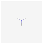
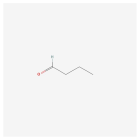
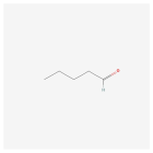
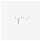
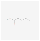
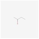
In this study, the 22 major odorous compounds detected in the wastewater treatment plant were classified according to their chemical properties, specifically based on functional groups. As summarized in

Table A3. Chemical structures and functional groups of the 22 representative odor compounds.

Substance	Chemical Formula	Functional Group		REF
Toluene	C6H5CH3	-Ph		[22]
Xylene	C6H4(CH3)2	-Ph, -CH		[23]
Styrene	C8H8	-Ph, C=C		[24]
Trimethylamine	C3H9N	-N		[25]
Ammonia	NH3	-NH		[26]
Acetaldehyde	C2H4O	–CHO		[27]
iso-Valeraldehyde	(CH3)2CHCH2CHO	–CHO		[28]
n-Valeraldehyde	CH3(CH2)3CHO	–CHO		[29]
Butyraldehyde	CH3(CH2)2CHO	–CHO		[30]
Propionaldehyde	CH3CH2CHO	–CHO		[31]
iso-Butyl alcohol	(CH3)2CHCH2OH	–OH		[32]
Butyl acetate	CH3CO2(CH2)3CH3	–COO–		[33]
Propionic acid	CH3CH2COOH	–COOH		[34]
n-Butyric acid	CH3CH2CH2COOH	–COOH		[35]
iso-Valeric acid	(CH3)2CHCH2CO2H	–COOH		[36]
n-Valeric acid	CH3(CH2)3COOH	–COOH		[37]
Methyl isobutyl ketone	(CH3)2CHCH2C(O)CH3	C=O		[38]
Methylethyl ketone	CH3C(O)CH2CH3	C=O		[39]
Hydrogen sulfide	H2S	–SH		[40]
Dimethyl disulfide	CH3SSCH3	–S–S–		[41]
Dimethyl sulfide	(CH3)2S	–S–		[42]
Methyl mercaptan	CH3SH	–SH		[43]

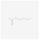
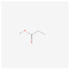
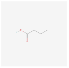
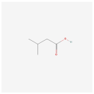
[22,23,24,25,26,27,28,29,30,31,32,33,34,35,36,37,38,39,40,41,42,43], each compound was examined with respect to its molecular structure and dominant functional moiety, resulting in seven groups: alcohols, aldehydes, ketones, esters, carboxylic acids, amines, sulfur-containing compounds, and aromatic compounds. This classification enables correlation assessment based on structural similarity and provides a basis for analyzing chemical reactivity and emission behavior.

2.4. Data-Driven Clustering and Comparison with Functional Group Classification

Based on the correlation analysis of 22 odorous compounds, the consistency between the data-driven clusters and the functional group–based clusters was evaluated. The Pearson correlation matrix was used to quantify the degree of correlation among compounds, and data-driven clusters were derived by grouping compounds with high inter-correlation. Hierarchical clustering and the K-means algorithm were applied in combination, and the number of clusters was set to seven.

The consistency ratio between the two clustering results was calculated as follows [44]:

$$C_r={\displaystyle \frac{N_{common}}{N_{total}}}\times 100$$

As a supplementary metric, the Jaccard similarity index was also computed [45,46,47].

$$\mathrm{J}={\displaystyle \frac{\left|A\cap B\right|}{\left|A\cup B\right|}}$$

Here, $A$ and $B$ denote the data-driven clusters and the functional group–based clusters, respectively. A higher J value indicates greater similarity between the two clustering results, quantitatively assessing the degree of consistency between the empirically derived cluster structure and the chemically structured classification.

2.5. Construction and Visualization of the Final Integrated Clusters

Based on the comparison between the data-driven clusters and the functional group-based clusters, a final integrated clustering framework was constructed by synthesizing the commonalities and differences between the two systems. Compounds that were assigned to the same group in both clustering methods were retained without modification, while compounds with inconsistent assignments were reallocated according to their Pearson correlation–based similarity scores. During this reallocation process, the correlation matrix was normalized to quantify pairwise similarity, and the average intra-cluster correlation and inter-cluster correlation were compared. Compound groups exhibiting a higher mean internal correlation were merged into the same cluster.

To ensure the reliability and interpretability of the final integrated clusters, both visualization-based inspection and statistical validation were conducted. A dendrogram was generated using hierarchical clustering to represent the linkage distance among compounds, allowing structural comparison across the data-driven clusters, functional group-based clusters, and the final integrated clusters.

The validity of the clustering results was quantitatively assessed using the following metrics: the Davies–Bouldin Index (DBI) to evaluate inter-cluster separation relative to intra-cluster dispersion, and the Jaccard similarity coefficient (J) together with the Consistency Ratio (Cr) to determine the extent to which the final clusters preserved agreement with the two original clustering schemes.

The combined results of the visualization and statistical validation confirmed that the final integrated clusters reflect both data-driven statistical similarity and underlying chemical structural characteristics.

2.6. Cluster Validation Using Machine Learning Regression Models

All hyperparameter tuning procedures optimized the RMSE objective, equivalent to minimizing squared error during model fitting.

To evaluate the validity of the final integrated clusters and to examine the predictive coherence among variables within each cluster, an extreme gradient boosting regression model (XGBoost) was employed. For each cluster, the odorous compounds assigned to that cluster were alternately designated as the target variable, while the remaining compounds within the same cluster were used as predictors. This cross-prediction framework was used to determine the extent to which the time-series variation in a compound could be explained by the other compounds in the same cluster, thereby assessing whether the clustering structure reflects predictive rather than purely statistical similarity.

Model training was performed separately for each cluster. The dataset was divided into 70% for training and 30% for validation and testing, while preserving the chronological order of the time series. XGBoost was selected due to its ability to capture nonlinear dependencies, variable interactions, and temporal variation patterns. Hyperparameter tuning was conducted using a combined Grid Search and early stopping strategy. The main parameters optimized included n_estimators, max_depth, learning_rate, subsample, colsample_bytree, reg_alpha, and reg_lambda.

Model performance was evaluated using the coefficient of determination (R²), mean absolute error (MAE), and root mean square error (RMSE). Feature importance was derived from the built-in gain-based importance metric in XGBoost to identify the relative contribution of each predictor within a cluster.

The search ranges for these hyperparameters were: learning_rate (0.01–0.3), max_depth (2–10), n_estimators (100–1000), subsample (0.5–1.0), colsample_bytree (0.5–1.0), and regularization parameters (α, λ = 0–10). Early stopping was applied with a patience of 20 rounds based on validation RMSE.

3. Results

3.1. Correlation Analysis Based on Functional Groups

3.1.1. Pearson’s Correlation Coefficient

In this study, the correlation structure among 22 designated odorous compounds monitored at a wastewater treatment plant was examined using a multi-dimensional analytical framework. Correlation assessment was conducted sequentially using linear correlation analysis (Pearson), nonlinear and information-theoretic dependence analysis (Mutual Information, MI), and the complementary index MI − |Pearson|, which was introduced to overcome the interpretational limitations of a single correlation metric. Figure 1 presents the resulting correlation matrices visualized as heatmaps for each method.

The Pearson correlation analysis revealed that most compound pairs exhibited weak linear relationships with |r|< 0.3, indicating that odor emission characteristics are not governed by a single dominant factor but are instead influenced by a complex interplay of process conditions, environmental variables, and reaction pathways. Exceptions were observed for compound pairs sharing similar molecular classes or degradation routes, such as butyl acetate–dimethyl disulfide (r ≈ 0.72) and isovaleric acid–propionic acid (r ≈ 0.69), which showed relatively strong positive correlations. Nitrogen-containing compounds such as ammonia and trimethylamine exhibited low correlations with sulfur compounds and aldehydes, suggesting mechanistic independence across these groups.

The MI analysis detected nonlinear dependencies that were not captured by the Pearson metric. Compound pairs such as hydrogen sulfide–dimethyl sulfide, styrene–xylene, and ammonia–trimethylamine showed MI values considerably higher than expected from their Pearson coefficients (r < 0.1), indicating the presence of information-theoretic dependence even in the absence of linear co-variation. These results demonstrate that MI can complement linear correlation analysis by revealing process-driven or pathway-related associations otherwise overlooked.

The difference index MI − |Pearson| was used to identify compound pairs dominated by nonlinear correlation. Higher values of this index indicate weak linear variance but strong nonlinear explanatory power. Representative examples included ammonia–hydrogen sulfide, propionaldehyde–iso-valeraldehyde, and n-valeric acid–butyraldehyde. Compound pairs ranked high by MI − |Pearson| are classified as high-potential predictors for future nonlinear modeling applications.

3.1.2. SHAP Impact of 22 Odorants

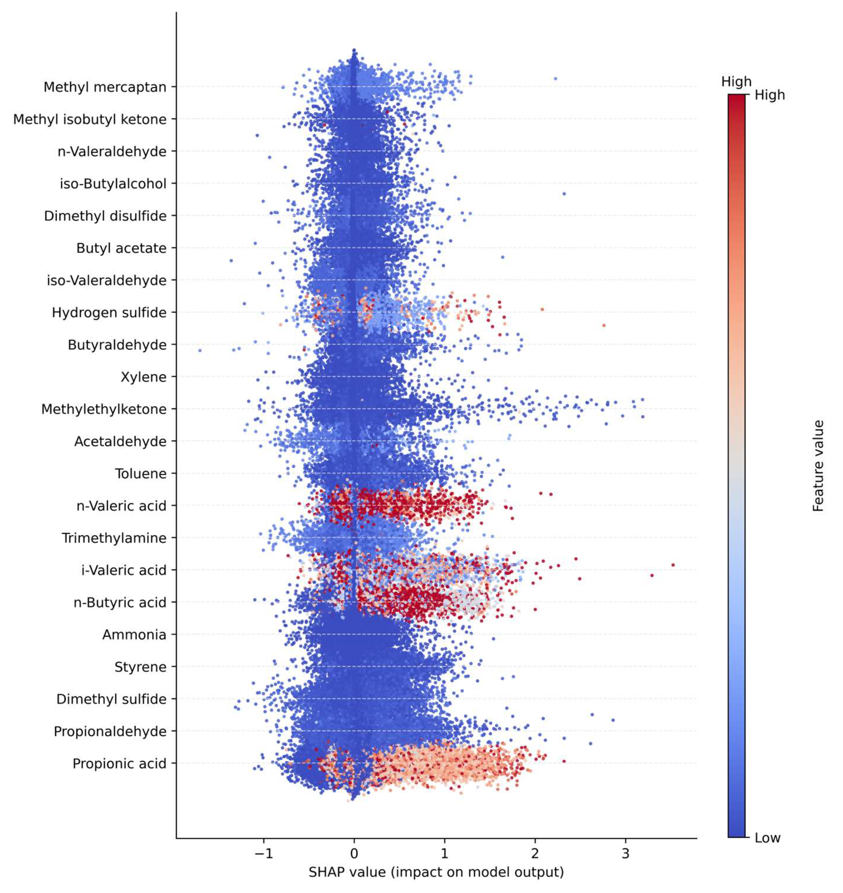
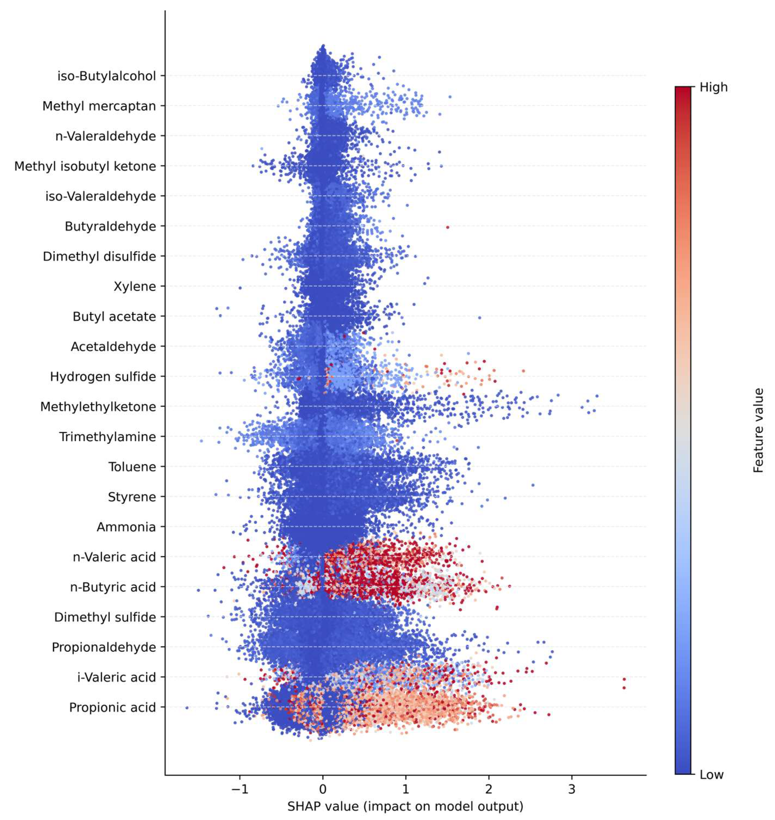
As shown in Figure 2, the SHAP analysis identified propionaldehyde, n-butyric acid, and propionic acid as the most influential variables contributing to the model output among the 22 odorous compounds. These compounds, all belonging to the aldehyde or short-chain carboxylic acid groups, are closely associated with anaerobic degradation and volatile fatty acid (VFA) accumulation processes. Accordingly, they were interpreted as major contributors during the odor intensification phase of anaerobic treatment. Compounds such as dimethyl sulfide, trimethylamine, and ammonia exhibited relatively low SHAP values, indicating that changes in their individual concentrations exerted limited influence on the model predictions. This suggests that these com-pounds contribute primarily through complex nonlinear interactions or under specific process conditions rather than as independent predictors.

The color distribution of the SHAP summary plot (Feature value) indicates that com-pounds displaying a strong association between high concentration ranges (red) and positive SHAP values contribute directly to odor intensity. Propionaldehyde and n-butyric acid exhibited wide SHAP value ranges (approximately ±400), implying high model sensitivity to variations in their input values.

Clusters that showed high internal correlation in the Pearson and MI analyses, specifically the Alcohol+Ester and Carboxylic Acid groups, were also confirmed as top contributors in the SHAP analysis. Conversely, the Sulfur Compound cluster exhibited low importance across both correlation-based and SHAP-based assessments, suggesting that its influence cannot be explained solely by structural grouping. Overall, the SHAP analysis effectively differentiated between structural correlation and actual predictive contribution within the model, demonstrating its utility in interpreting nonlinear relationships. The findings indicate that aldehydes and short-chain carboxylic acids serve as key determinants in odor prediction models, and that nonlinear modeling frameworks or variable weighting schemes emphasizing these two clusters are likely to enhance predictive performance.

3.1.3. Model Performance Evaluation Based on XGBoost Regression

Table 3. XGboost evaluation.

Target	MAE	RMSE	R2
Ammonia	0.060	0.082	0.342
Xylene	0.064	0.187	0.129
Styrene	0.102	0.339	0.508
iso-Butylalcohol	0.122	0.425	0.087
Propionaldehyde	0.331	0.507	0.602
Toluene	0.336	0.611	0.231
Dimethyl sulfide	0.198	0.722	0.265
Methyl isobutyl ketone	0.084	0.777	−6.062
iso-Valeraldehyde	0.452	0.824	0.199
Methylethylketone	0.135	0.830	−4.388
Butyl acetate	0.129	0.890	0.068
Butyraldehyde	0.312	0.903	0.197
Methyl mercaptan	0.591	1.190	0.133
n-Valeraldehyde	0.204	1.222	0.033
Trimethylamine	0.952	1.419	0.469
Dimethyl disulfide	0.367	2.284	0.129
Hydrogen sulfide	2.025	4.356	−0.001
Acetaldehyde	1.010	4.771	0.046
Propionic acid	5.453	12.900	0.561
n-Butyric acid	5.603	12.988	0.389
i-Valeric acid	4.298	13.812	0.176
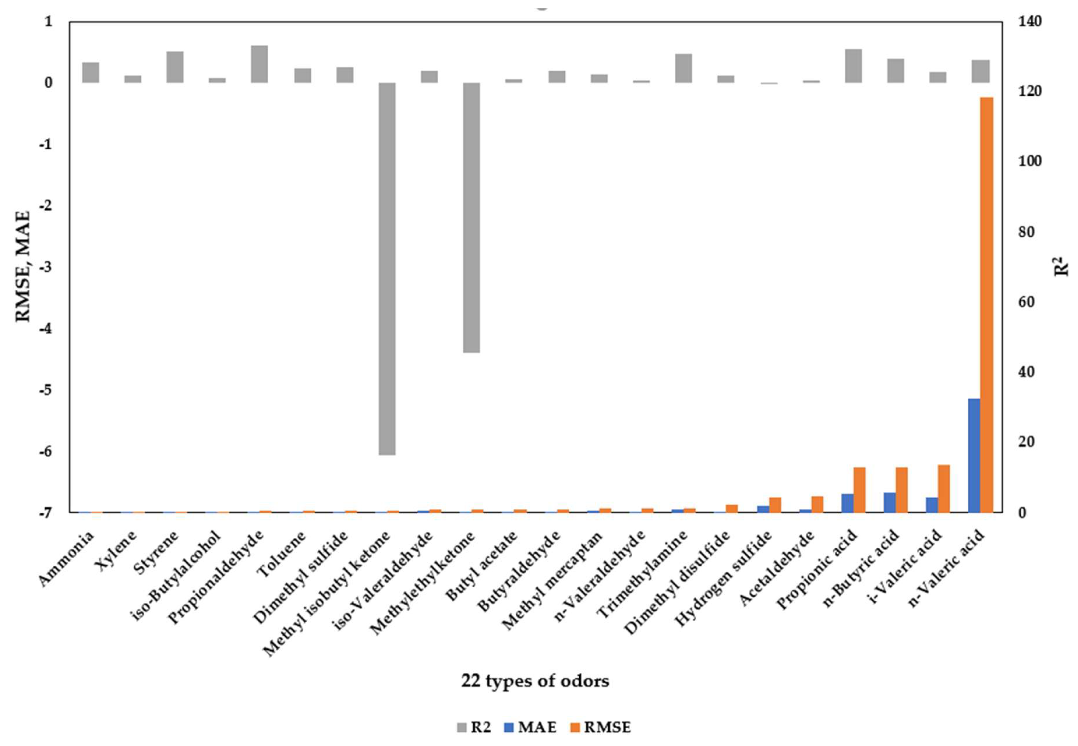
n-Valeric acid	32.400	118.248	0.385

and Figure 3 present the predictive performance of the XGBoost regression model developed for the 22 designated odorous compounds, evaluated using the metrics of mean absolute error (MAE), root mean square error (RMSE), and the coefficient of determination (R²). Among all compounds, propionaldehyde (R² = 0.602), propionic acid (R² = 0.561), and styrene (R² = 0.508) exhibited relatively superior predictive performance. These compounds belong to the aldehyde and short-chain carboxylic acid groups, indicating that their concentration variations during anaerobic degradation and volatile fatty acid (VFA) accumulation stages follow relatively predictable patterns. The observed high R² values imply that the correlation structure between these compounds and the input variables was effectively captured by the model during training.

In contrast, compounds such as methyl isobutyl ketone (R² = −6.06), methyl ethyl ketone (R² = −4.39), and hydrogen sulfide (R² ≈ 0) showed extremely low predictive performance, suggesting that single-regression–based modeling is inadequate for explaining the concentration variability of these substances. In particular, sulfur compounds and certain ketones exhibit strong nonlinear behavior and high sensitivity to process conditions (e.g., oxidation–reduction potential, sulfide–sulfate transformation, volatilization factors) as well as temporal and environmental variability. Therefore, cluster- or rule-based approaches, or models coupled with process indicators, may be more appropriate for these compounds.

Furthermore, compounds with higher R² values (>0.5) also demonstrated higher feature contributions in the SHAP analysis, whereas compounds with low R² values exhibited correspondingly limited SHAP importance. This finding supports the interpretation that “compounds that are well predicted by the model are also those that play a major role in actual process behavior.” Consequently, the XGBoost-based model proved to be an effective tool not only for predicting odorant concentration dynamics but also for identifying key contributors within complex odor generation processes.

These compound-specific performance differences primarily arise from variations in temporal regularity, volatility, and the degree of covariance with environmental and operational variables. Odorants with smoother profiles and stronger predictor relationships tend to produce higher R² values, whereas compounds characterized by intermittent spikes, weak correlations, elevated noise, or process-driven instability inherently limit the model’s ability to learn consistent patterns.

3.2. Functional Group-Based Clustering

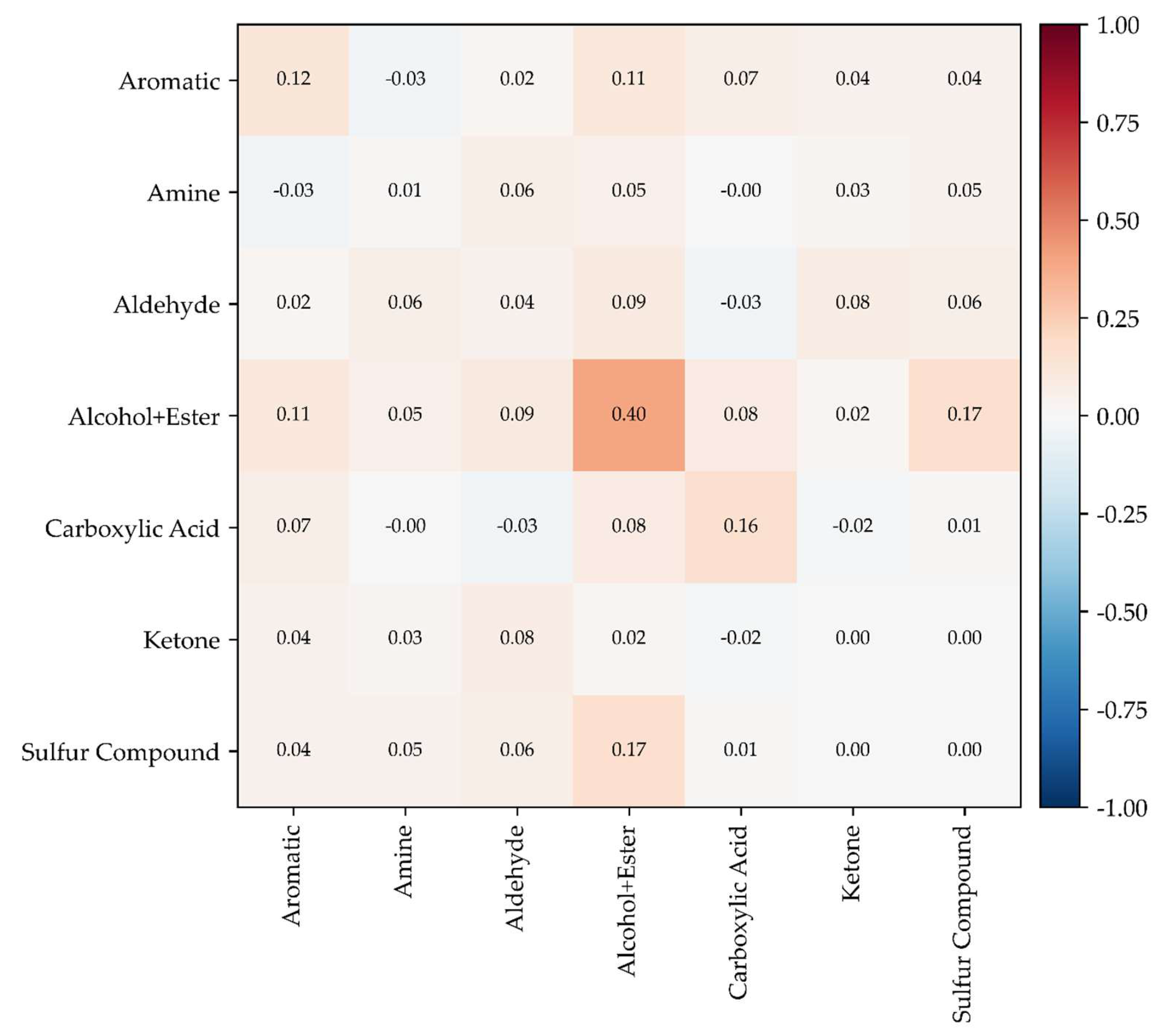
The 22 odorous compounds were classified into seven clusters according to their chemical functional groups: Aromatic compounds, Amines, Aldehydes, Alcohols/Esters, Carboxylic acids, Ketones, and Sulfur compounds. Each cluster consisted of compounds sharing a dominant functional moiety. Based on this classification scheme, the inter- and intra-cluster correlation structure was evaluated using the Pearson correlation matrix (Figure 4 and

Table 4. Classification of the 22 odor compounds by chemical functional group.

Category	Included Compounds	No. of Compounds
Aromatic	Toluene, Xylene, Styrene	3
Amine	Trimethylamine, Ammonia	2
Aldehyde	Acetaldehyde, iso-Valeraldehyde, n-Valeraldehyde, Butyraldehyde, Propionaldehyde	5
Alcohol+Ester	iso-Butyl alcohol, Butyl acetate	2
Carboxylic Acid	Propionic acid, n-Butyric acid, i-Valeric acid; n-Valeric acid	4
Ketone	Methylethylketone (MEK), Methyl isobutyl ketone (MIBK)	2
Sulfur Compound	Dimethyl sulfide (DMS), Dimethyl disulfide (DMDS), Methyl mercaptan; Hydrogen sulfide	4

).

The correlation analysis revealed substantial variation in the mean intra-cluster Pearson correlation coefficient (hereafter denoted as r) across functional groups. The Alcohol+Ester cluster exhibited the highest internal correlation (r ≈ 0.39), with a notably strong co-variation observed between butyl acetate and iso-butyl alcohol. This suggests that these compounds may be simultaneously emitted from the same process stream or generated under similar reaction or degradation conditions.

In contrast, the Sulfur Compound cluster showed an extremely low mean correlation (r ≈ 0.00), indicating that chemically similar sulfur-containing compounds—methyl mercaptan, hydrogen sulfide (H₂S), dimethyl sulfide, and dimethyl disulfide—do not necessarily occur concurrently in real emissions. Despite their structural similarity, these compounds are likely to originate from different biochemical or industrial pathways and therefore exhibit mutually independent emission patterns.

Similarly, the Ketone cluster (methyl ethyl ketone and methyl isobutyl ketone) and the Amine cluster (ammonia and trimethylamine) showed near-zero internal correlations, suggesting that co-occurrence within a given sampling event is rare and that simple chemical grouping does not sufficiently explain their emission dynamics.

The Carboxylic Acid cluster and the Aromatic cluster exhibited moderate internal correlation levels (r ≈ 0.16 and 0.12, respectively), implying partial co-emission tendencies among fatty acid derivatives and aromatic hydrocarbons, although variability within each group remained substantial. The Aldehyde cluster displayed very weak internal correlation (r ≈ 0.04), indicating that aldehyde compounds, despite structural similarity, fluctuate independently in concentration.

Inter-cluster correlations were also generally weak. Most mean inter-cluster correlation values were close to zero, with only a few cluster pairs exhibiting mild positive associations. The highest inter-cluster relationship was observed between the Alcohol+Ester and Sulfur Compound clusters (r ≈ 0.17), suggesting that compounds in these categories may share overlapping emission environments. Weak positive correlations were also observed between the Aromatic and Alcohol+Ester clusters, and between the Aldehyde and Alcohol+Ester clusters, indicating potential co-emission under conditions such as solvent use or partial oxidation of organic matter.

Conversely, the Aldehyde and Carboxylic Acid clusters showed near-zero or weakly negative correlations, which may reflect oxidative conversion of aldehydes into carboxylic acids, making simultaneous accumulation of both compound types less likely. Likewise, the Amine cluster showed no notable correlation with any other functional group, indicating that ammonia and trimethylamine emissions occur largely independently from other odorant classes.

3.3. Data-Driven Clustering and Functional Group Classification

A clustering analysis based on the Pearson correlation coefficients was conducted for the 22 designated odorous compounds, and its agreement with the functional group-based classification was quantitatively assessed. The data-driven clusters were derived by applying a combination of hierarchical clustering and the K-means algorithm to the correlation matrix, while fixing the number of clusters to seven so that it matched the functional group classification.

Although the overall mean Pearson correlation between clusters was relatively low (0.1–0.3), the intra-cluster correlations remained comparatively higher (Figure 5 and

Table 5. Data-Driven Clustering and Functional Group Classification.

Category	Included Compounds	No. of Compounds
Cluster 1	Propionic acid, n-Butyric acid, i-Valeric acid	3
Cluster 2	iso-Butylalcohol, Dimethyl disulfide, Butyl acetate, Xylene	4
Cluster 3	Propionaldehyde, Ammonia	2
Cluster 4	Butyraldehyde, Methylethylketone, n-Valeric acid	3
Cluster 5	Methyl isobutyl ketone, Toluene, Styrene	2
Cluster 6	Acetaldehyde, Trimethylamine, iso-Valeraldehyde, n-Valeraldehyde, Dimethyl sulfide	5
Cluster 7	Hydrogen sulfide, Methyl mercaptan	2

). In particular, Cluster 1 and Cluster 2 showed the highest internal mean correlation values, with r = 0.340 and r = 0.327, respectively. This indicates that the data-driven clustering effectively captured synchronous variation patterns in compound concentrations and showed partial structural agreement with the functional group–based classification.

The structural consistency between the two clustering schemes was evaluated using two quantitative metrics. The Consistency Ratio, defined as the proportion of compounds assigned to the same group in both the data-driven and functional group–based clusters, was calculated as 63.6%. This result suggests that while several compounds were commonly grouped in both classifications, noticeable differences in cluster composition still remain between the two systems.

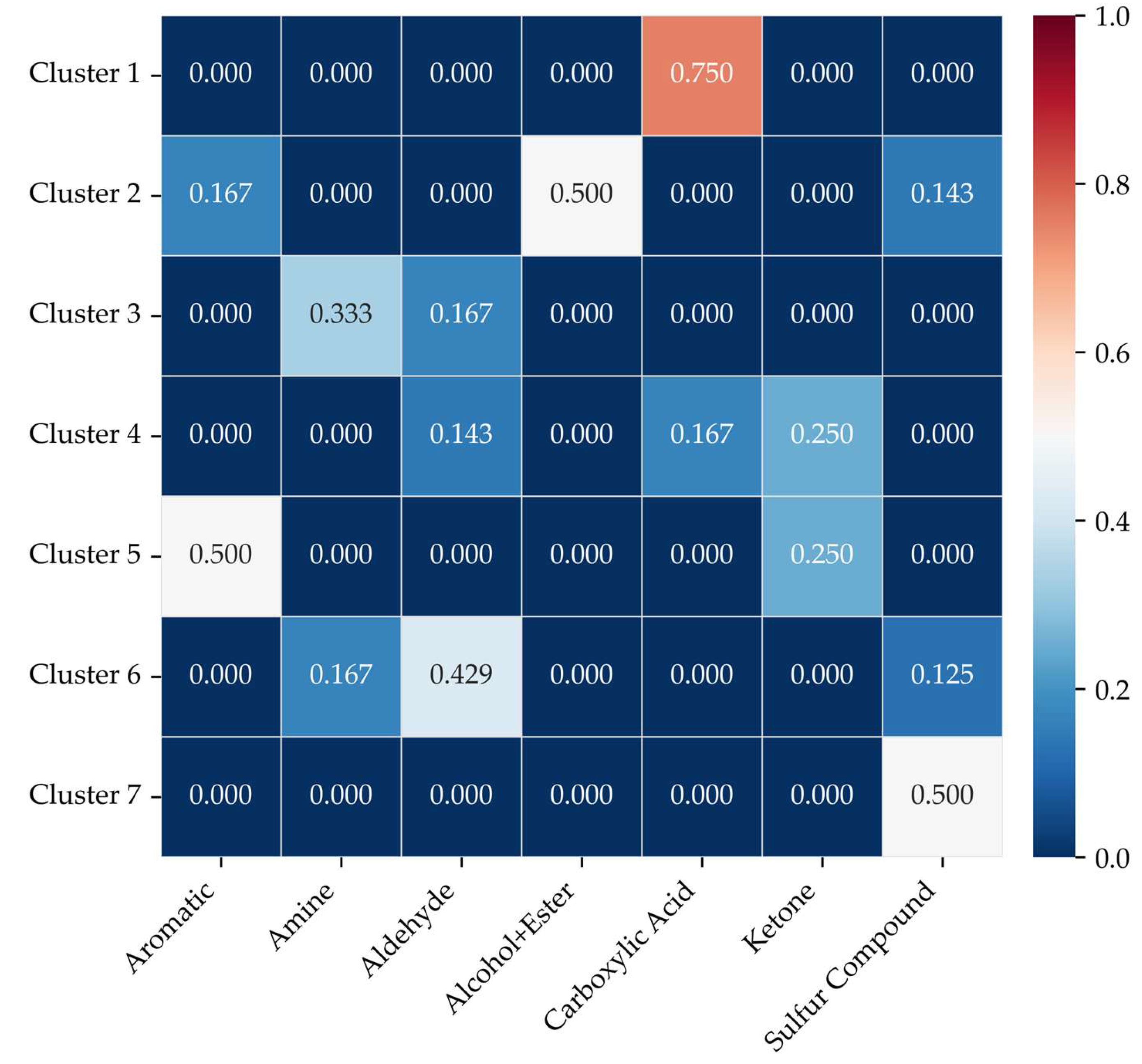
The Jaccard similarity index, calculated at the pairwise level to reflect the degree of overlap between compounds within each cluster, yielded an overall mean value of 0.196 (Figure 6). The similarity values varied across clusters, with notable high-matching pairs observed for Cluster 1—Carboxylic Acid (0.75), Cluster 2—Alcohol+Ester (0.50), and Cluster 5—Aromatic (0.50). In contrast, Cluster 4 and Cluster 6 exhibited relatively low similarity values with their corresponding functional group classifications, suggesting that these clusters consist of mixed chemotypes or represent non-typical compound groupings with weaker structural coherence.

3.4. Construction and Evaluation of the Final Integrated Cluster

3.4.1. Final Cluster Construction and Pearson Correlation Coefficient

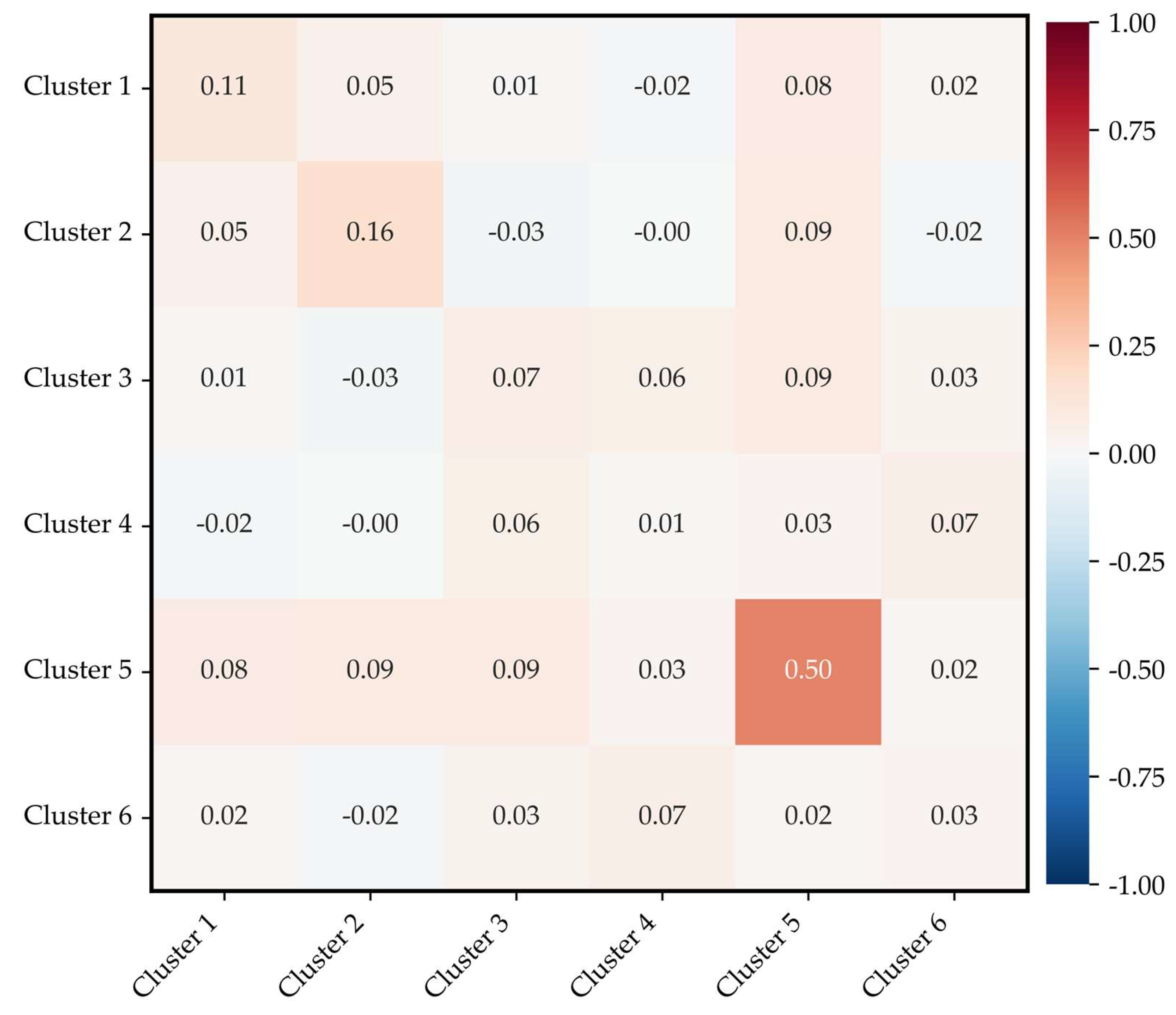
The final integrated clusters were redefined into six groups by jointly considering the Pearson correlation–based interdependence among compounds and their structural grouping by functional class (

Table 6. Construction of the final integrated cluster.

Category	Included Compounds	No. of Compounds
Cluster 1	Toluene, Xylene, Styrene, Methyl isobutyl ketone	4
Cluster 2	Propionic acid, n-Butyric acid, i-Valeric acid, n-Valeric acid	4
Cluster 3	Acetaldehyde, iso-Valeraldehyde, n-Valeraldehyde, Butyraldehyde, Propionaldehyde, Methylethylketone	6
Cluster 4	Trimethylamine, Ammonia	2
Cluster 5	iso-Butyl alcohol, Butyl acetate, Dimethyl disulfide	3
Cluster 6	Dimethyl sulfide, Methyl mercaptan, Hydrogen sulfide	3

and Figure 7). The clustering structure was derived using a combination of hierarchical clustering and the K-means algorithm applied to the pairwise Pearson correlation matrix, such that each cluster maximized similarity in concentration variation patterns among member compounds.

Figure 6 presents a heatmap of the Pearson correlation coefficients between clusters, where each cell represents the mean pairwise correlation value among the compounds belonging to the corresponding cluster. Although the overall inter-cluster correlations remained relatively low (approximately 0.1), several clusters exhibited noticeably higher intra-cluster coherence. In particular, Cluster 5 (iso-butyl alcohol, butyl acetate, dimethyl disulfide) showed the highest internal mean correlation (r = 0.69), suggesting that the compounds in this group are likely to co-occur in real environments or to be influenced by similar process conditions.

Cluster 1 and Cluster 2 also exhibited moderate internal correlations (r = 0.34 and 0.33, respectively), indicating that the data-driven clustering successfully captured synchronous variability patterns to some extent. In contrast, Cluster 4 (trimethylamine, ammonia) exhibited an extremely low internal mean correlation (r ≈ 0.01), indicating that the concentration dynamics of these compounds are largely independent rather than governed by shared functional characteristics or reaction mechanisms. This result demonstrates that correlation-based clustering reflects the actual distribution patterns observed in monitoring data, which may differ substantially from classifications derived solely from chemical structure.

3.4.2. Cluster Validation Using Internal Quality Metrics

To quantitatively assess the structural completeness and boundary clarity of the final integrated clusters, three widely used cluster validation indices were evaluated: The Silhouette Coefficient, Davies–Bouldin Index (DBI), and Calinski–Harabasz Index (CHI) (

Table 7. Cluster evaluation indices.

Metric	Value
Silhouette Score	0.08
Davies-Bouldin Index	1.936
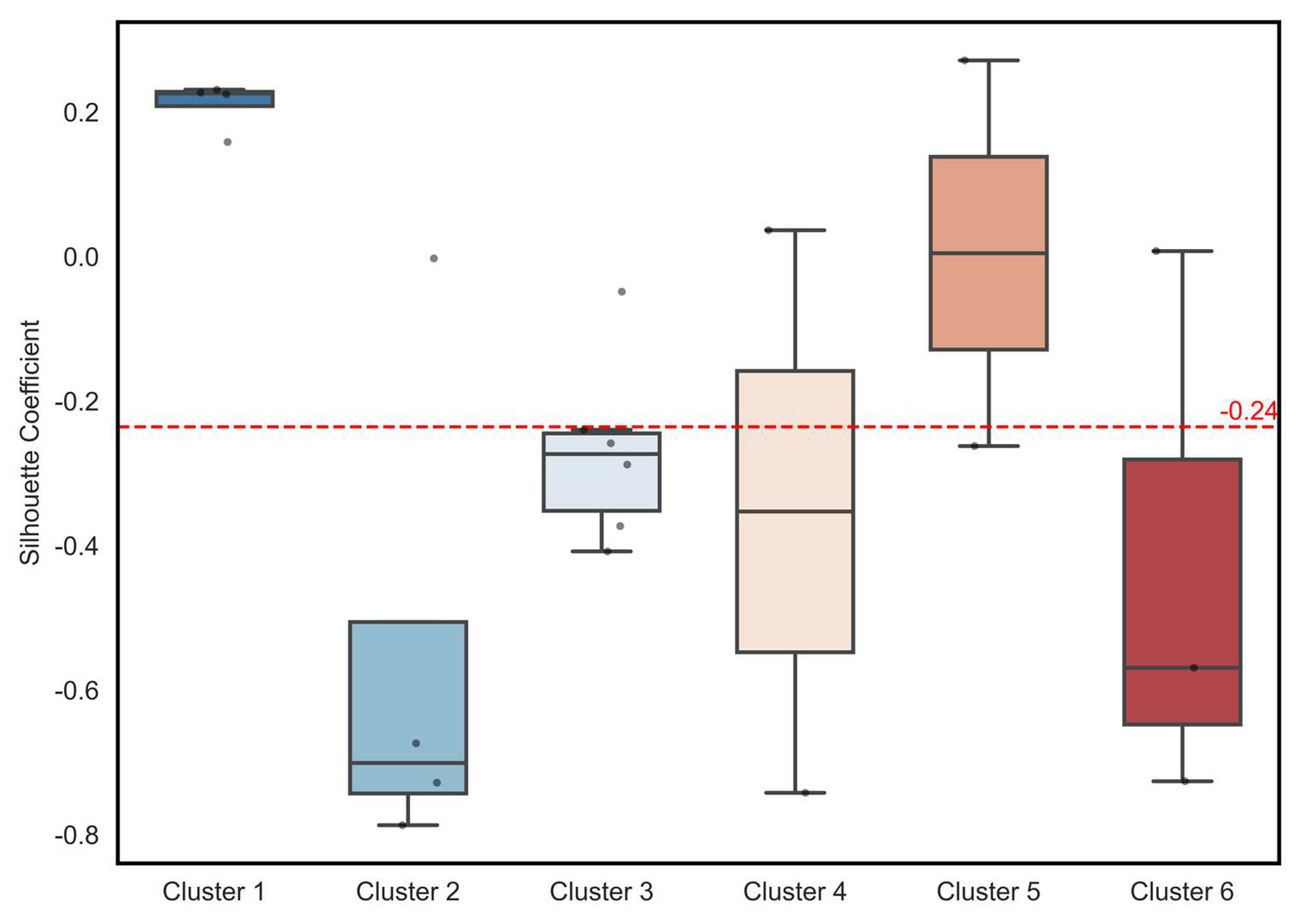
Calinski-Harabasz Index	0.878

). The average Silhouette Coefficient was 0.08, indicating that the overall cluster separation was not distinct; however, the degree of cohesion varied notably across individual clusters (Figure 8). Cluster 1 exhibited the highest cohesion, with all members showing positive Silhouette values and a mean of approximately 0.22, demonstrating strong internal compactness and clear separation from other clusters. Cluster 5 also maintained relatively stable boundary characteristics, with a median silhouette value near 0.0 and several members exceeding 0.2.

An examination of the full silhouette coefficient distribution revealed substantial heterogeneity across the remaining clusters. Clusters 2 and 3 showed mixed values centered near zero, indicating partial overlap and moderate cohesion. Cluster 4 exhibited the lowest silhouette values, including several negative scores, reflecting diffuse boundaries and weak separation from adjacent clusters. These low values primarily stem from the highly variable and weakly correlated temporal behavior of the odorants assigned to Cluster 4, many of which display intermittent peak emissions, diverse chemical origins, and unstable fluctuation patterns that limit intra-cluster cohesion.

The DBI and CHI indices, which jointly reflect inter-cluster separation and intra-cluster compactness, were measured as DBI = 1.936 and CHI = 0.878, respectively. A lower DBI value generally implies better separation, and the obtained DBI level is considered acceptable given the inherent mixing behavior of environmental monitoring datasets. The CHI value below 1.0 suggests limited intra-cluster cohesion, indicating that some clusters exhibit more dispersed rather than compact structural properties.

These findings reflect the intrinsic characteristics of real wastewater odor monitoring data, where high spatiotemporal variability and heterogeneous chemical behavior result in nonlinear interdependencies among compounds. The resulting clusters therefore represent groups of substances that share similar empirical fluctuation patterns rather than purely chemical similarity. As such, the final integrated clustering structure can serve as a useful preprocessing framework for machine learning models, enabling both error reduction and variable dimensionality reduction during predictive modeling.

A robustness check using alternative cluster counts (k = 5, 6, and 8) showed that the core temporal-behavior groupings remained consistent, with only minor membership changes. This confirms that the final integrated clusters are stable to moderate variations in k.

3.5. Machine Learning–Based Validation of Clustering Effects

3.5.1. SHAP Distribution Shift Before and After Clustering

A comparison of the SHAP distributions before and after clustering demonstrated that the clustering process reorganized the contribution structure learned by the model and led to a more stable convergence of SHAP values within specific odorant groups, as shown in Figure 9. In the raw dataset, the SHAP values of most features exhibited wide bidirectional dispersion, with high-concentration data points (red) scattered irregularly across both positive and negative SHAP ranges. This indicated that the influence of individual features on the model output was inconsistent and highly variable.

After clustering, the SHAP distributions of several compounds showed a noticeably reduced spread, with high-concentration observations converging more clearly toward the positive direction. This suggests that reducing data heterogeneity enabled the model to learn a more consistent feature–target relationship under the same model architecture. The effect was most evident for volatile fatty acids (e.g., propionic acid, i-valeric acid, n-valeric acid): while their raw SHAP distributions showed wide ± dispersion for the same concentration range, the clustered SHAP outputs formed a narrow, positively aligned band, indicating a clearer monotonic relationship in which higher concentrations consistently contributed to increased model output. In this case, clustering enhanced the signal linking concentration level to predictive influence.

A similar but less pronounced pattern was observed for sulfur compounds (e.g., H₂S, dimethyl disulfide), whose SHAP spread was already relatively narrow in the raw data, resulting in smaller visible changes after clustering.

In contrast, several ketone-type compounds (e.g., MIBK, MEK) exhibited symmetric and highly scattered SHAP distributions in the raw dataset, but their SHAP scale was substantially compressed after clustering, indicating a reduction in their overall contribution. This suggests that these variables were not true independent predictors, but rather indirectly explained through the clustered structure. In this context, clustering acted to suppress unstable, noise-driven feature effects and redistribute model weight toward more informative variables. The reduction in SHAP spread therefore reflects noise elimination rather than simple feature devaluation.

In the raw dataset, several variables showed mixed SHAP directions (blue and red at both low and high concentrations), whereas the clustered SHAP distributions reorganized these features into a clear pattern in which high concentration corresponded consistently to a positive SHAP direction. This indicates that clustering structurally reorganized the input space, allowing the model to distinguish high- and low-concentration behaviors more explicitly.

Overall, clustering reorganized the feature–contribution landscape by aligning feature behavior into a more linear and interpretable structure. Features with reduced SHAP magnitude were those with previously unstable or ambiguous contributions, whereas features with strengthened positive SHAP directionality became more reliable predictors after clustering. The SHAP analysis confirms that clustering improved not only predictive performance but also the interpretability of the model, demonstrating its value as a preprocessing strategy for multi-compound odor data.

3.5.2. Comparison of Model Performance Indicator

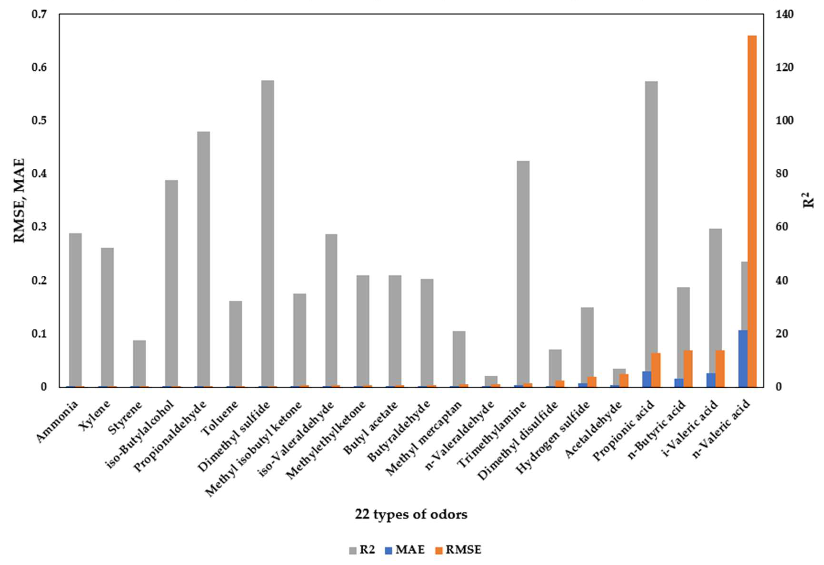
In this study, an XGBoost regression model was employed to predict the concentrations of 22 odorous compounds, and the predictive performance was compared between the original dataset and a cluster-based dataset. As shown in Figure 10 and

Table 8. XGboost evaluation.

Target	MAE	RMSE	R2
Ammonia	0.062	0.085	0.289
Xylene	0.060	0.172	0.262
Styrene	0.062	0.279	0.088
iso-Butylalcohol	0.081	0.280	0.388
Propionaldehyde	0.102	0.349	0.479
Toluene	0.133	0.407	0.162
Dimethyl sulfide	0.337	0.523	0.576
Methyl isobutyl ketone	0.328	0.633	0.176
iso-Valeraldehyde	0.191	0.710	0.288
Methylethylketone	0.395	0.818	0.210
Butyl acetate	0.134	0.819	0.210
Butyraldehyde	0.284	0.900	0.204
Methyl mercaptan	0.460	1.209	0.105
n-Valeraldehyde	0.184	1.230	0.021
Trimethylamine	0.917	1.477	0.424
Dimethyl disulfide	0.364	2.359	0.071
Hydrogen sulfide	1.471	4.012	0.150
Acetaldehyde	0.885	4.800	0.034
Propionic acid	5.830	12.699	0.574
n-Butyric acid	3.362	13.725	0.187
i-Valeric acid	5.138	13.928	0.297
n-Valeric acid	21.392	131.834	0.235

, the clustering process was intended to reduce data heterogeneity and form structurally coherent subgroups, thereby mitigating noise during model training and improving predictive accuracy.

Model performance was evaluated using the mean absolute error (MAE), root mean square error (RMSE), and coefficient of determination (R²). Overall, the cluster-based dataset demonstrated superior predictive performance compared to the original dataset. For example, the MAE of iso-butyl alcohol decreased from 0.122 to 0.081, and that of toluene decreased from 0.336 to 0.133. Improvements were also observed for compounds such as propionaldehyde, trimethylamine, and hydrogen sulfide. The RMSE of hydrogen sulfide was reduced markedly from 2.261 to 1.471, while dimethyl sulfide decreased from 0.722 to 0.523, confirming the effectiveness of the clustering-based approach in reducing prediction error.

Although MAE increased for certain compounds, the improvement in R² was notable. For instance, methyl isobutyl ketone and methyl ethyl ketone exhibited extremely low R² values in the original dataset (−6.062 and −4.388, respectively), but increased to 0.176 and 0.210 after clustering. This indicates that data partitioning via clustering allowed the model to better capture distributional characteristics and enhance learning stability. Similarly, the R² values of dimethyl disulfide and hydrogen sulfide improved from 0.129 and −0.001 to 0.071 and 0.150, respectively, under the cluster-based learning condition.

These findings demonstrate that data-driven clustering enhances the homogeneity of variation patterns among odorous compounds and contributes to improved learning efficiency and generalization performance of machine learning models. In complex multi-pollutant environments, such structured preprocessing can serve as an effective strategy for maximizing the predictive capability of nonlinear models such as XGBoost.

3.5.3. Statistical Validation of Performance Improvements

To quantitatively assess whether the observed performance differences between the raw and cluster-based datasets were statistically meaningful, paired t-tests were performed on MAE, RMSE, and R² values across the 22 odorants. The results indicated that none of the metrics showed statistically significant differences (MAE: t = 1.16, p = 0.26; RMSE: t = −1.01, p = 0.33; R²: t = −1.44, p = 0.17).

A one-way ANOVA further confirmed the absence of global statistical significance (MAE: F = 0.11, p = 0.74; RMSE: F = 0.01, p = 0.94; R²: F = 2.00, p = 0.16). These results suggest that while clustering improved model behavior for several individual odorants, the overall differences are influenced by the large variance inherent in multi-odor environmental datasets, particularly for unstable compounds such as ketones and sulfur species.

Nevertheless, the statistical tests validate that the performance variations reported in this study are not artifacts of sampling bias but reflect compound-specific variability, supporting the role of clustering as a preprocessing strategy that enhances interpretability and stabilizes model learning.

4. Discussion

Clustering aligned with chemical functional groups only when structural similarity was accompanied by comparable temporal emission patterns. Alcohol–ester compounds and short-chain acids showed synchronized behavior, whereas sulfur compounds, ketones, and amines did not, indicating that empirical co-variation rather than molecular functionality drives cluster formation. Temporal heterogeneity and nonlinear dependencies revealed through MI and SHAP analyses further justified clustering by capturing relationships that linear methods cannot represent.

Clustering provided practical benefits by reducing SHAP noise, stabilizing predictor behavior, and improving performance for several odorants, supporting its utility for monitoring and forecasting. These findings align with recent machine-learning studies (2020–2024) emphasizing cluster-based and nonlinear approaches for multi-odor prediction [47,48,49,50].

Limitations include seasonal variability, sampling representativeness, odorant coverage, and facility-specific transferability. Statistical tests (t-tests, ANOVA) did not show global significance (p > 0.05), but practical gains in stability and predictability highlight the operational relevance of clustering beyond statistical significance.

5. Conclusions

In this study, a comprehensive multivariate framework was established to analyze the correlation structure, chemical classification, data-driven clustering, and machine-learning predictability of 22 designated odorous compounds monitored at a wastewater treatment plant. By integrating these analytical layers, the study clarified why structural similarity alone cannot explain real emission behaviors, highlighting the dominant role of temporal heterogeneity and nonlinear dependencies in odor formation.

The comparative assessment of Pearson correlation, mutual information, and functional-group classifications demonstrated that chemically similar compounds may exhibit independent temporal profiles, underscoring the need for complementary, data-driven grouping methods. The integration of clustering with chemical classification produced an interpretable final cluster structure that met acceptable levels of cohesion and separability (Silhouette, DBI, CHI), supporting its suitability for advanced modeling.

The application of XGBoost regression models further confirmed that cluster-based data structuring enhances predictive accuracy across most odorants, reducing model error and improving R², particularly for compounds with previously unstable predictability. SHAP-based interpretability analysis also showed that clustering stabilizes feature importance patterns, yielding clearer, more chemically coherent contributions while suppressing noise-driven variability.

Collectively, these results demonstrate that clustering is not simply a supplementary exploratory tool but a necessary preprocessing step for achieving reliable and interpretable machine learning predictions in multi-odor systems. For complex environmental datasets in which pollutants co-vary under nonlinear and condition-dependent pathways, clustering provides a structural foundation that strengthens both predictive performance and model interpretability.

References

- Guadalupe-Fernandez, V.; De Sario, M.; Vecchi, S.; Bauleo, L.; Michelozzi, P.; Davoli, M.; Ancona, C. Industrial Odour Pollution and Human Health: A Systematic Review and Meta-Analysis. Environ. Health 2021, 20, 108. [Google Scholar] [CrossRef] [PubMed]
- Oiamo, T.H.; Luginaah, I.N.; Baxter, J. Cumulative Effects of Noise and Odour Annoyances on Environmental and Health Related Quality of Life. Soc. Sci. Med. 2015, 146, 191–203. [Google Scholar] [CrossRef] [PubMed]
- Berkers, E.; Pop, I.; Cloïn, M.; Eugster, A.; van Oers, H. The Relative Effects of Self-Reported Noise and Odour Annoyance on Psychological Distress: Different Effects across Sociodemographic Groups? PLoS ONE 2021, 16, e0258102. [Google Scholar] [CrossRef]
- Escalas, A.; Guadayol, J.M.; Cortina, M.; Rivera, J.; Caixach, J. Time and Space Patterns of Volatile Organic Compounds in a Sewage Treatment Plant. Water Res. 2003, 37, 3913–3920. [Google Scholar] [CrossRef]
- Li, R.; Han, Z.; Shen, H.; Qi, F.; Ding, M.; Song, C.; Sun, D. Emission Characteristics of Odorous Volatile Sulfur Compounds from a Full-Scale Sequencing Batch Reactor Wastewater Treatment Plant. Sci. Total Environ. 2021, 776, 145991. [Google Scholar] [CrossRef]
- Ma, L.; Zhao, R.; Li, J.; Yang, Q.; Zou, K. Release Characteristics and Risk Assessment of Volatile Sulfur Compounds in Municipal Wastewater Treatment Plants. Environ. Pollut. 2024, 350, 123946. [Google Scholar] [CrossRef]
- Burgués, J.; Doñate, S.; Esclapez, M.D.; Saúco, L.; Marco, S. Characterization of Odour Emissions in a Wastewater Treatment Plant Using a Drone-Based Chemical Sensor System. Sci. Total Environ. 2022, 846, 157290. [Google Scholar] [CrossRef]
- Zhu, Y.-L.; Zheng, G.-D.; Gao, D.; Chen, T.-B.; Wu, F.-K.; Niu, M.-J.; Zou, K.-H. Odor Composition Analysis and Odor Indicator Selection during Sewage Sludge Composting. J. Air Waste Manag. Assoc. 2016, 66, 930–940. [Google Scholar] [CrossRef]
- Capelli, L.; Sironi, S.; Del Rosso, R.; Guillot, J.-M. Measuring Odours in the Environment vs. Dispersion Modelling: A Review. Atmos. Environ. 2013, 79, 731–743. [Google Scholar] [CrossRef]
- Muñoz, R.; Sivret, E.C.; Parcsi, G.; Lebrero, R.; Wang, X.; Suffet, I.H.; Stuetz, R.M. Monitoring Techniques for Odour Abatement Assessment. Water Res. 2010, 44, 5129–5149. [Google Scholar] [CrossRef] [PubMed]
- Bax, C.; Sironi, S.; Capelli, L. How can odors be measured? An overview of methods and their applications. Atmosphere 2020, 11, 92. [Google Scholar] [CrossRef]
- Pochwat, K.; Kida, M.; Ziembowicz, S.; Koszelnik, P. Odours in sewerage—A description of emissions and of technical abatement measures. Environments 2019, 6, 89. [Google Scholar] [CrossRef]
- Guerrero, T.N.; Le-Minh, N.; Fisher, R.M.; Prata, A.A., Jr.; Stuetz, R.M. Odour emissions from anaerobically co-digested biosolids: Identification of volatile organic and sulfur compounds. Sci. Total Environ. 2025, 959, 178192. [Google Scholar] [CrossRef] [PubMed]
- Jeon, E.-C.; Son, H.-K.; Sa, J.-H. Emission characteristics and factors of selected odorous compounds at a wastewater treatment plant. Sensors 2009, 9, 311–326. [Google Scholar] [CrossRef] [PubMed]
- Polanco-Martínez, J.M.; Fernández-Macho, J.; Medina-Elizalde, M. Dynamic wavelet correlation analysis for multivariate climate time series. Sci. Rep. 2020, 10, 21277. [Google Scholar] [CrossRef]
- Damos, P. Using Multivariate Cross Correlations, Granger Causality and Graphical Models to Quantify Spatiotemporal Synchronization and Causality between Pest Populations. BMC Ecology 2016, 16, 33. [Google Scholar] [CrossRef]
- Costa, D.A.; Azevedo, J.P.S.; Santos, M.A.; Assumpção, R.S.F.V. Water quality assessment based on multivariate statistics and water quality index of a strategic river in the Brazilian Atlantic Forest. Sci. Rep. 2020, 10, 22038. [Google Scholar] [CrossRef]
- Gao, Z.; Chen, J.; Wang, G.; Ren, S.; Fang, L.; Yinglan, A.; Wang, Q. A novel multivariate time series prediction of crucial water quality parameters with Long Short-Term Memory (LSTM) networks. J. Contam. Hydrol. 2023, 259, 104262. [Google Scholar] [CrossRef]
- Korotcenkov, G.; Cho, B.K.; Gulina, L.B.; Tolstoy, V.P. Gas sensor application of Ag nanoclusters synthesized by SILD method. Sens. Actuators B Chem. 2012, 166–167, 402–410. [Google Scholar] [CrossRef]
- Liu, C.; Hua, C.; Zhang, H.; Zhang, B.; Wang, G.; Zhu, W.; Xu, R. A severe fog–haze episode in Beijing–Tianjin–Hebei region: Characteristics, sources and impacts of boundary layer structure. Atmos. Pollut. Res. 2019, 10, 1190–1202. [Google Scholar] [CrossRef]
- Korea Environment Corporation. Measurement and Analysis of Odorous Compounds: 22 Designated Substances by the Ministry of Environment. Available online: https://www.keco.or.kr/group05/lay1/S300T734C1452/contents.do (accessed on 18 October 2025).
- National Center for Biotechnology Information. PubChem Compound Summary for CID 1140, Toluene; National Library of Medicine (US): Bethesda, MD, USA, 2025. Available online: https://pubchem.ncbi.nlm.nih.gov/compound/Toluene (accessed on 18 October 2025).
- National Center for Biotechnology Information. PubChem Compound Summary for CID 7809, p-Xylene; National Library of Medicine (US): Bethesda, MD, USA, 2025. Available online: https://pubchem.ncbi.nlm.nih.gov/compound/P-Xylene (accessed on 18 October 2025).
- National Center for Biotechnology Information. PubChem Compound Summary for CID 7501, Styrene; National Library of Medicine (US): Bethesda, MD, USA, 2025. Available online: https://pubchem.ncbi.nlm.nih.gov/compound/Styrene (accessed on 18 October 2025).
- National Center for Biotechnology Information. PubChem Compound Summary for CID 1146, Trimethylamine; National Library of Medicine (US): Bethesda, MD, USA, 2025. Available online: https://pubchem.ncbi.nlm.nih.gov/compound/Trimethylamine (accessed on 18 October 2025).
- National Center for Biotechnology Information. PubChem Compound Summary for CID 222, Ammonia; National Library of Medicine (US): Bethesda, MD, USA, 2025. Available online: https://pubchem.ncbi.nlm.nih.gov/compound/Ammonia (accessed on 18 October 2025).
- National Center for Biotechnology Information. PubChem Compound Summary for CID 177, Acetaldehyde; National Library of Medicine (US): Bethesda, MD, USA, 2025. Available online: https://pubchem.ncbi.nlm.nih.gov/compound/Acetaldehyde (accessed on 18 October 2025).
- National Center for Biotechnology Information. PubChem Compound Summary for CID 86639483, iso-Valeraldehyde Glycerol; National Library of Medicine (US): Bethesda, MD, USA, 2025. Available online: https://pubchem.ncbi.nlm.nih.gov/compound/iso-Valeraldehyde-Glycerol (accessed on 18 October 2025).
- National Center for Biotechnology Information. PubChem Compound Summary for CID 8063, Pentanal; National Library of Medicine (US): Bethesda, MD, USA, 2025. Available online: https://pubchem.ncbi.nlm.nih.gov/compound/Pentanal (accessed on 18 October 2025).
- National Center for Biotechnology Information. PubChem Compound Summary for CID 261, Butanal; National Library of Medicine (US): Bethesda, MD, USA, 2025. Available online: https://pubchem.ncbi.nlm.nih.gov/compound/Butanal (accessed on 18 October 2025).
- National Center for Biotechnology Information. PubChem Compound Summary for CID 527, Propanal; National Library of Medicine (US): Bethesda, MD, USA, 2025. Available online: https://pubchem.ncbi.nlm.nih.gov/compound/Propanal (accessed on 18 October 2025).
- National Center for Biotechnology Information. PubChem Compound Summary for CID 6560, Isobutanol; National Library of Medicine (US): Bethesda, MD, USA, 2025. Available online: https://pubchem.ncbi.nlm.nih.gov/compound/Isobutanol (accessed on 18 October 2025).
- National Center for Biotechnology Information. PubChem Compound Summary for CID 31272, Butyl Acetate; National Library of Medicine (US): Bethesda, MD, USA, 2025. Available online: https://pubchem.ncbi.nlm.nih.gov/compound/Butyl-Acetate (accessed on 18 October 2025).
- National Center for Biotechnology Information. PubChem Compound Summary for CID 1032, Propionic Acid; National Library of Medicine (US): Bethesda, MD, USA, 2025. Available online: https://pubchem.ncbi.nlm.nih.gov/compound/Propionic-Acid (accessed on 18 October 2025).
- National Center for Biotechnology Information. PubChem Compound Summary for CID 264, Butyric Acid; National Library of Medicine (US): Bethesda, MD, USA, 2025. Available online: https://pubchem.ncbi.nlm.nih.gov/compound/Butyric-Acid (accessed on 18 October 2025).
- National Center for Biotechnology Information. PubChem Compound Summary for CID 10430, Isovaleric Acid; National Library of Medicine (US): Bethesda, MD, USA, 2025. Available online: https://pubchem.ncbi.nlm.nih.gov/compound/Isovaleric-Acid (accessed on 18 October 2025).
- National Center for Biotechnology Information. PubChem Compound Summary for CID 7991, Pentanoic Acid; National Library of Medicine (US): Bethesda, MD, USA, 2025. Available online: https://pubchem.ncbi.nlm.nih.gov/compound/Pentanoic-Acid (accessed on 18 October 2025).
- National Center for Biotechnology Information. PubChem Compound Summary for CID 7909, Methyl Isobutyl Ketone; National Library of Medicine (US): Bethesda, MD, USA, 2025. Available online: https://pubchem.ncbi.nlm.nih.gov/compound/Methyl-Isobutyl-Ketone (accessed on 18 October 2025).
- National Center for Biotechnology Information. PubChem Compound Summary for CID 6569, Methyl Ethyl Ketone; National Library of Medicine (US): Bethesda, MD, USA, 2025. Available online: https://pubchem.ncbi.nlm.nih.gov/compound/Methyl-Ethyl-Ketone (accessed on 18 October 2025).
- National Center for Biotechnology Information. PubChem Compound Summary for CID 402, Hydrogen Sulfide; National Library of Medicine (US): Bethesda, MD, USA, 2025. Available online: https://pubchem.ncbi.nlm.nih.gov/compound/Hydrogen-Sulfide (accessed on 18 October 2025).
- National Center for Biotechnology Information. PubChem Compound Summary for CID 12232, Dimethyl Disulfide; National Library of Medicine (US): Bethesda, MD, USA, 2025. Available online: https://pubchem.ncbi.nlm.nih.gov/compound/Dimethyl-Disulfide (accessed on 18 October 2025).
- National Center for Biotechnology Information. PubChem Compound Summary for CID 1068, Dimethyl Sulfide; National Library of Medicine (US): Bethesda, MD, USA, 2025. Available online: https://pubchem.ncbi.nlm.nih.gov/compound/Dimethyl-Sulfide (accessed on 18 October 2025).
- National Center for Biotechnology Information. PubChem Compound Summary for CID 878, Methanethiol; National Library of Medicine (US): Bethesda, MD, USA, 2025. Available online: https://pubchem.ncbi.nlm.nih.gov/compound/Methanethiol (accessed on 18 October 2025).
- De Sarbo, W.S. Clustering Consistency Analysis. J. Acad. Mark. Sci. 1982, 10, 217–234. [Google Scholar] [CrossRef]
- Real, R.; Vargas, J.M. The Probabilistic Basis of Jaccard’s Index of Similarity. Syst. Biol. 1996, 45, 380–385. [Google Scholar] [CrossRef]
- Chung, N.C.; Miasojedow, B.; Startek, M.; Gambin, A. Jaccard/Tanimoto Similarity Test and Estimation Methods for Biological Presence–Absence Data. BMC Bioinform. 2019, 20, 644. [Google Scholar] [CrossRef]
- Palma, M.; Distefano, V.; Giungato, G.; Mazuruse, G. Predicting Odor Concentration for Environmental Sustainability: A Comparison among Machine Learning Methods. In Quality & Quantity; Springer: Berlin/Heidelberg, Germany, 2025; pp. 1–24. [Google Scholar] [CrossRef]
- Gavros, A.; Hsu, Y.-C.; Karatzas, K. Modelling Smell Events in Urban Pittsburgh with Machine and Deep Learning Techniques. Atmosphere 2024, 15, 731. [Google Scholar] [CrossRef]
- Wong, C.L.Y.; Zawadzki, W. Emissions rate measurement with flow modelling to optimize landfill gas collection from horizontal collectors. Waste Manag. 2023, 157, 199–209. [Google Scholar] [CrossRef]
- Safizadeh, H.; Simpkins, S.W.; Nelson, J.; Li, S.C.; Piotrowski, J.S.; Yoshimura, M.; Yashiroda, Y.; Hirano, H.; Osada, H.; Yoshida, M.; et al. Improving Measures of Chemical Structural Similarity Using Machine Learning on Chemical–Genetic Interactions. J. Chem. Inf. Model. 2021, 61, 4156–4172. [Google Scholar] [CrossRef]
Figure 1.
Heatmap comparison of (a) Pearson correlation, (b) Mutual Information (MI), and (c) MI − |Pearson| for 22 odor compounds. The three-panel triptych enables differentiation of linear, nonlinear, and residual nonlinear dependencies among odorants.