Article

A Multi-Objective Optimization Study of Supply Air Parameters in a Supersonic Aircraft Cabin Environment Combined with Fast Calculation

1
College of Urban Construction, Nanjing Tech University, Nanjing 211816, China
2
School of Safety Science and Engineering (School of Emergency Management), Nanjing University of Science and Technology, Nanjing 210094, China
3
Defense Engineering Institute, AMS, People’s Liberation Army of China, Beijing 100036, China
4
Tianmushan Laboratory, Hangzhou 310023, China
5
School of Aeronautic Science and Engineering, Beihang University, Beijing 100191, China
*
Author to whom correspondence should be addressed.
Atmosphere 2025, 16(9), 1005; https://doi.org/10.3390/atmos16091005
Submission received: 7 July 2025 / Revised: 17 August 2025 / Accepted: 21 August 2025 / Published: 25 August 2025
(This article belongs to the Section Atmospheric Techniques, Instruments, and Modeling)

Abstract

Supersonic cabins are characterized by high heat flux and high occupant density, which can adversely affect passenger comfort, health, and energy efficiency. This study proposed a multi-objective optimization framework for determining supply air parameters in a supersonic aircraft cabin, evaluating the performances of different optimization methods. The optimization focused on three design objectives: thermal comfort (PMV), air freshness (air age), and the temperature differential between the supply and exhaust air. Two fast calculation methods—Proper Orthogonal Decomposition (POD) and Artificial Neural Networks (ANN)—were compared alongside two optimization algorithms: Multi-Objective Genetic Algorithm (MOGA) and Pareto search. The results indicate that the POD method has a smaller relative root mean square error compared to the ANN method. The relative root mean square error of the ANN method in predicting PMV is 2.7 times higher than the POD method and 3.9 times higher in air age prediction. The Pareto search algorithm outperformed MOGA in computational efficiency, generating 3.3 times more Pareto-optimal solutions in less time. The entropy weight method was used to assign weight for both optimization algorithms, revealing that neither algorithm achieved universally optimal performance across all objectives. Therefore, selecting the best solution requires aligning optimization outcomes with specific design priorities.

1. Introduction

Supersonic civil aircraft is one of the most disruptive civil aircraft products in the high-end main track of international competition for future large passenger aircraft [1]. The United States, Europe and other aviation powerhouses are accelerating new generation of supersonic aircraft to return to sky as shown in Figure 1. Moreover, green supersonic civil aircraft design technology is also one of the 20 cutting-edge science and engineering technology problems by the China Association for Science and Technology. Air travel now serves over 2 billion passengers annually [2], which brings multiple challenges for aircraft environmental control systems (ECS). Without proper management, the ECS may consume excessive energy, and passengers may experience thermal discomfort due to overcooling or overheating, thereby compromising the overall in-flight comfort. Another concern is the lack of effective airflow organization within the cabin, which can lead to the rapid spread of harmful substances, posing significant health risks to passengers. For example, the outbreak of the coronavirus disease during air travel in 2019 caused considerable disruption and damage. Teleszewski et al. and Mariita et al.’s research also shows that ECS plays an important role in regulating comfort and health in the cabin [3,4]. These issues reveal underlying shortcomings within current cabin ventilation systems and airflow arrangements, underscoring the urgent need for optimization and redesign.
Compared with ordinary cabins, supersonic aircraft cabins have greater heat flux, more occupant density and higher energy consumption, and there is a lack of framework on the optimal design of supply air parameters in supersonic aircraft cabins. For the optimization design for the cabin environment, it mainly has two parts: the fast calculation method and the optimization algorithm. The fast calculation method is used to calculate the physical fields distributions based on the dataset of design variables, and the optimization algorithm is used to filter out the optimal solutions included in the dataset.
Many scholars have studied the optimization of cabin and indoor ventilation systems, with the multi-objective genetic algorithm (MOGA) being one of the most commonly used optimization algorithms. The MOGA is often combined with other computational methods to enhance optimization design, with the most frequent combination being MOGA and computational fluid dynamics (CFD). For example, Zhai et al. employed a CFD method based on MOGA for optimizing three design objectives—PMV (predicted mean vote), PD (percentage dissatisfied), and the air age—within both two-dimensional office and three-dimensional cabin environments [7]. With the advancement of fast fluid dynamics, Xue et al. integrated fast fluid dynamics with GA, achieving superior computational efficiency compared to the traditional GA-CFD approach [8]. Additionally, some researchers have combined the MOGA with fast computational methods. For instance, Zhang et al. combined MOGA with ANN, demonstrating a successful optimization of ventilation systems [9]. Overall, the MOGA method offers distinct advantages in solving optimization problems.
Pareto search is also an optimization algorithm, which has been the subject of many studies. For instance, Bjelic et al. utilized the Pareto search algorithm to optimize the design of a dual-ellipsoidal heat source used in the calibration of a 3-D quasi-steady-state heat transfer model for gas-shielded metal arc welding [10]. The optimization process involved five input parameters, with simulation results compared against experimental observations. The results demonstrated a good agreement between the simulated and experimental values of the heat source model. Similarly, Al-Ghussain et al. applied the Pareto search algorithm for multi-objective optimization in renewable energy systems (RES), where the design objectives included the RES fraction, the demand-supply fraction (DSF) and the levelized cost of electricity as a key factor [11]. These findings suggest that the Pareto search algorithm offers distinct advantages in solving multi-objective optimization problems as well.
Another commonly used optimization method is the adjoint method. This method involves updating the design variables and continuously calculating the objective functions. The objective function then moves along the gradient direction, which ultimately minimizes the function [12]. The adjoint method can be combined with fast calculation methods. For instance, Liu et al. applied the adjoint method with fast fluid dynamics, which significantly reduces the computational time of simulations [13]. Zhao et al. integrated area-restricted topology and cluster analysis within the CFD adjoint method, enabling the determination of key parameters for the ventilation system, including the number, location, size, and even the shape of the air outlets [14]. Zhao et al. improved the uniformity of the air vents in the cockpit by combining the adjoint method and genetic algorithm [15]. Although the adjoint method is effective, it can be prone to falling into localized solutions, which limits its applicability in some cases. For the MOGA and Pareto search algorithms, though these two methods have been widely studied, there is still a lack of comparative analysis of their optimization performances for supply air parameters in the tight supersonic cabin with high heat flux density and occupant density.
For the calculation method, the traditional method for calculating airflow and temperature distributions is the CFD method, which utilizes an iterative computational approach to solve the Navier–Stokes (N-S) equations. However, CFD is not sufficiently fast when used as a computational method for rapid calculations in optimization processes. Faster and more efficient methods are required to address these challenges. Artificial Neural Network (ANN) and Proper Orthogonal Decomposition (POD) are commonly used as fast calculation methods, which can significantly enhance computational efficiency. The POD method is used to reduce dimensionality through spatial correlation, and the flow field at a specific location is then derived by interpolation. Various sampling methods can be employed in POD interpolation. Xu et al. proposed a local density sampling approach, which samples more densely in complex physical environments to improve the accuracy of the POD interpolation [16]. Different interpolation techniques also can be applied in the POD calculation process. Wei et al. employed the POD linear interpolation method to degrade and interpolate the angle and temperature of the inlet gas, enabling the rapid generation of the flow field under unknown boundary conditions for subsequent optimization calculations in aircraft cabins [17]. Liang et al. used a POD-based method to optimize the attached ventilation parameters of high-altitude buildings [18]. Besides aircraft cabins and rooms, the POD method has also been employed in train cabin environment. Lu et al. used the POD method to investigate the flow field of a high-speed train [19]. They employed Radial Basis Function (RBF) for interpolation, demonstrating that the POD method, when coupled with RBF interpolation, saves 99% of computational time compared to the CFD method.
For the ANN method, it has been introduced to reconstruct indoor airflow fields in recent years and demonstrated high accuracy. They are frequently combined with other modeling approaches. Wei et al. incorporated a Physics-Informed Neural Network (PINN) in their experiments, and the results confirmed that PINN is an effective meshless method, even when the inlet and outlet boundary conditions are unknown [20]. ANN has also been applied to optimize indoor environments. Zhang et al. utilized ANN alongside numerical simulations to propose a composite index that measures air resistance to pollutants, offering practical insights for environmental design [21]. Similarly, Zhao et al. employed ANN to enhance the separation efficiency of fats and oils, improving the kitchen environment [22]. Wang et al. used the radial basis function to optimize the air supply structure of the ventilation system and improved the comfort of the ankles of the indoor members [23].
Both the POD and ANN approaches have been extensively studied and applied for indoor environment optimization. However, there remains a gap in the comparative analysis of these two methods, particularly in terms of their computational performances and problem-solving accuracy, under the challenging conditions of supersonic cabins characterized by high heat flux density and occupant density. The main contributions of this study are summarized as follows:
(1) An optimization framework was developed for determining optimal supply air parameters in a supersonic aircraft cabin. The performance of POD and ANN were evaluated in predicting airflow patterns and temperature fields.
(2) A comparative analysis was conducted between MOGA and Pareto search, focusing on their computational speed and the distribution of Pareto frontier solutions.
(3) The entropy weight method was applied to determine the optimal solutions from both optimization algorithms. The distributions of PMV and air age for optimal and randomly selected design variables were analyzed, leading to practical design recommendations for enhanced cabin environmental quality and energy efficiency.

2. Material and Methods

2.1. Overviews

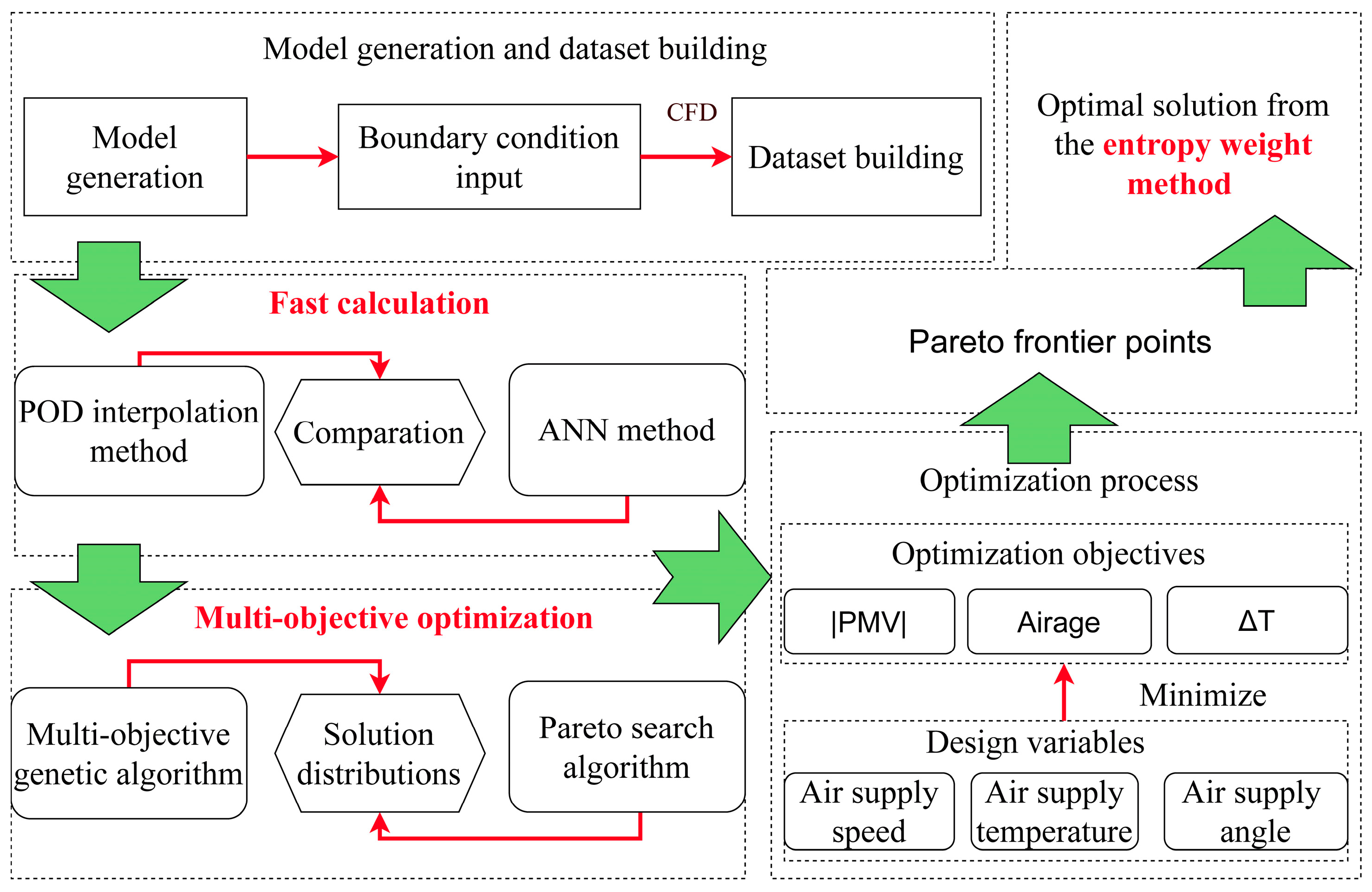
This study consists of three parts: model generation and dataset building, fast calculation, and multi-objective optimization. Figure 2 shows the multi-objective optimization framework of this study.
In the model generation and dataset building stage, the geometry and mesh of the aircraft cabin were generated, and different air supply boundary conditions within the design range were defined. Subsequently, after validation with the experimental data in the literature, various cases under different boundary conditions were conducted using CFD simulation. These simulations built the dataset required for the fast calculation model training. For the fast calculation stage, two fast calculation methods (POD and ANN) were employed to calculate the optimization objectives under any boundary conditions within the design range. Their relative errors were compared, and the more accurate method was selected for subsequent optimization.
For the multi-objective optimization stage, the MOGA and the Pareto search algorithm were utilized to approach the optimization objectives by adjusting the air supply design variables. The Pareto frontier solutions obtained from both algorithms were compared in terms of computational cost and solution distribution. Finally, the entropy weight method was applied to assign weight values and identify the optimal solutions.

2.2. Numerical Simulation of Cabin Environment

2.2.1. Numerical Model

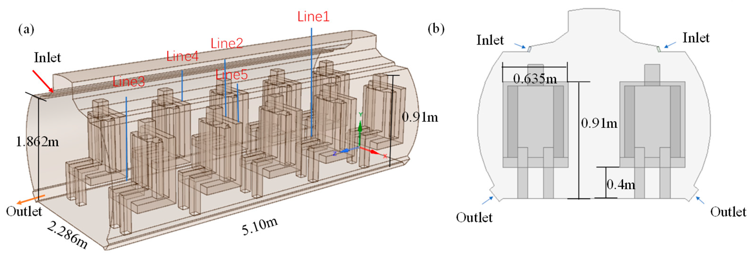
In this study, a numerical model was employed based on the cabin dimensions of the supersonic small airliner, the Concorde [24]. The cabin dimensions are 2.29 m (width) × 5.10 m (length) × 1.86 m (height), with five rows and two columns, a total of 10 seats. The heating mankind in the cabin is represented by a seated human model, with a height of 0.91 m corresponding to the vertical distance from the feet to the head when the person is seated [25]. The detailed view of the cabin and human models are shown in Figure 3.
The CFD process was carried out using FLUENT 2022R2, with the RNG k-ε turbulence model [26] for airflow simulation. The SIMPLE algorithm was used to handling the pressure-velocity coupling, and the second-order upwind scheme was used for discretizing all variables. Accounting for the buoyancy effect, the Boussinesq approximation was applied.

2.2.2. Determination of Boundary Conditions

To simulate the airflow within the aircraft cabin accurately, detailed diffuser model was typically required. However, overly complex diffuser structures could complicate the meshing process. Some simplified air supply models were often used, although these may lose some of the original geometric details, leading to potential discrepancies in airflow velocities. Therefore, it is essential to employ a suitably simplified air supply diffuser model that accurately represents the real air supply system.
In this study, a momentum-based air supply diffuser model was adopted, which preserved the essential characteristics of the original diffuser. It was achieved by introducing a momentum source on the air supply diffuser, compensating for the momentum of the airflow [27]. The momentum source value required for the simplified diffuser can be calculated using Equation (1).
S = ρ A s U s U r e a l U s V c e l l
U r e a l and U are the real and superficial velocities of the diffuser, A s is the superficial area of the diffuser, ρ is the density of the fluid, V c e l l is the volume of the momentum source cells on the diffuser.
Due to the higher cruising speed of supersonic aircraft compared to conventional aircraft, the friction with the air results in higher temperature of the inner cabin wall. The temperature of the outer cabin wall typically ranges between 127 °C and 91 °C, with the nose of the aircraft experiencing the highest temperature and the tail the lowest [28]. Based on the work of Zhang et al. [29] the temperature of the inner wall can be calculated by applying the thermal conductivity equation in Equation (2)
q l = t 1 t 2 1 2 π i = 1 3 1 λ i l n r i + 1 r i = h 1 2 π r 1 ( t i n t 1 )
where q l is the heat flow rate per unit length, t 1 and t 2 are the inner and outer wall temperatures, λ i and r i is the thermal conductivity of the i-th layer of insulation and the distance from the center of the nacelle in the heat-conducting layer, h 1 is the convective heat transfer coefficient between the inner wall and the air side, t i n is the indoor temperature. Finally, the temperature of the inner wall was 40 °C. In addition, the sensible heat dissipation rate of each passenger in the cabin is 76 W [30]. The grid size at the human body is 0.009 m, and the grid size in the middle of the cabin space is 0.04 m. The near-wall averaged Y plus value was 11, and the Scalable wall function was used in the simulation. The detailed boundary condition settings for this study are shown in Table 1.

2.2.3. Grid Independence Verification

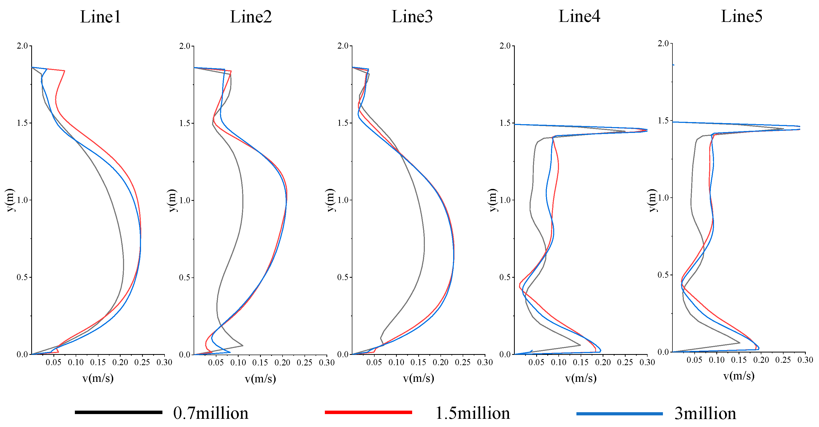
To determine the appropriate mesh density for the cabin simulation, three different mesh resolutions—0.6 million, 1.5 million, and 3 million mesh grids—were employed for mesh independence verification. During the meshing process, the grid resolution was refined in key areas, including the diffuser, outlet, and human models. Once the grids were defined, the simulation results for airflow velocity at five locations were compared across the three mesh cases, as shown in Figure 4. Lines 1, 2, and 3 are positioned in the middle of the aisle, while Lines 4 and 5 are located in the narrower region in front of the third row of passengers (Figure 3). As the grid density increases, the airflow velocity for the 1.5 million and 3 million grids follows similar trends; however, slight differences in velocity values are observed at Line 1 and Line 4 between the 1.5 million and 3 million grids. Overall, we conclude that the 1.5 million grid satisfies the mesh independence criteria and was selected for the subsequent calculations.

2.2.4. Validation with the Experimental Data in the Literature

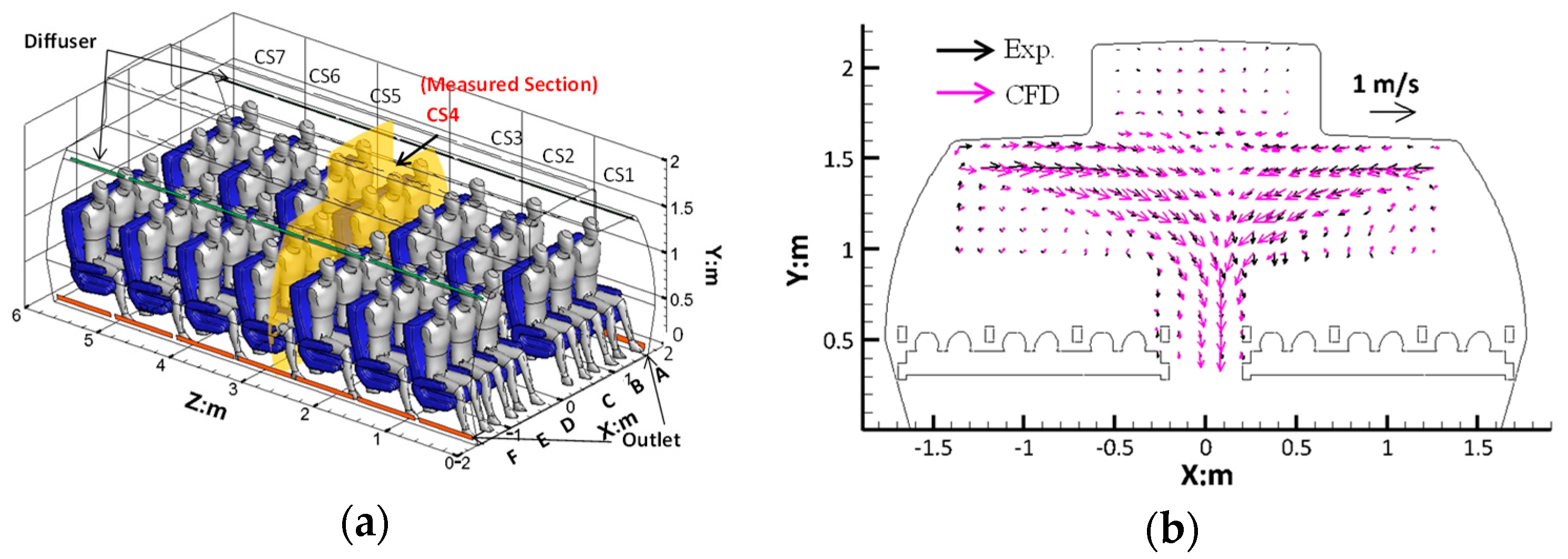
Since supersonic airliners currently in service are relatively scarce, it is not feasible to perform experimental validation specifically for supersonic aircraft cabins. Therefore, experimental data from conventional aircraft cabins reported in the literature were employed to validate the numerical model. Figure 5a illustrates the measurement section of the aircraft cabin, while Figure 5b presents a comparison between the predicted velocity field computed using the RNG k-ε turbulence model and experimental velocity field obtained via particle image velocimetry (PIV). Detailed descriptions of the experimental setup and numerical configurations can be found in Li et al. [31] and Li et al. [32], respectively. As shown in Figure 5b, the RNG k-ε model effectively captures the main flow features observed in the PIV measurements. Specifically, the airflow jets from the two side diffusers converge near the cabin centerline, and lower velocity magnitudes are observed near the ceiling and sidewall regions. Therefore, the RNG k-ε model can be used for numerical simulation in this study.

2.3. Fast Calculation Method

2.3.1. POD Method

The POD [33] method involves identifying a set of basic functions for the spatial model, onto which the original dataset can be projected in a manner that preserves the essential features of the original data as much as possible. CFD simulations were conducted to calculate the physical fields (e.g., velocity, concentration, temperature, etc.) corresponding to various boundary conditions. The results of these simulations were recorded in a matrix form. Subsequently, the matrix is downscaled using the POD method. To clarify this process, the airflow velocity matrix is expressed as follows:
U = u j = 1 i = 1 u j = 1 i = 2 u j = 1 i = m = u j = 1 i = 1 u j = 2 i = 1 . . . u j = n 1 i = 1 u j = n i = 1 u j = 1 i = 2 u j = 2 i = 2 . . . u j = n i = 2 u j = 1 i = m u j = 2 i = m u j = n i = m
where n is the number of samples and m is the number of grids for a particular airflow velocity field. Then the spatial model φ i can be determined by Equations (4) and (5).
S v = 1 n U U T v = λ v
E P = i = 1 P λ i / i = 1 N λ i
In Equation (4), where λ is the eigenvalue, v is the eigenvector, and S is the autocorrelation matrix corresponding to U . In Equation (5), where P is the number of the first P eigenvalues arranged from largest to smallest, which is also the number of spatial models seized, and N is the total number of eigenvalues.
In the process of POD dimensionality reduction, it is necessary to reduce the dimensionality as much as possible to reduce computational time but also need to retain the components of the original physical field as much as possible in order to retain the accuracy of the results. The contribution of the eigenvalues is used to select the number of eigenvectors to be retained, and generally the degree of retention of 99% can be a better result. The value of P corresponding to a contribution of 99% is the dimension to be retained in the POD method. P spatial modes φ i form a basis set. We used Equation (6) to project the original matrix onto this set of bases, and the corresponding spatial parameters can be obtained.
b i = φ i U φ i 2
where b i is the projection of the original velocity field onto the ith spatial mode. We could get P projection values, which were the spatial parameters of the POD downscaling method. The spline interpolation method was employed to interpolate the spatial parameters to derive the airflow velocity under unknown boundary conditions. According to Equation (7), we can reconstruct the velocity under the unknown boundary conditions. U ¯ is the velocity average value of U with respect to the rows.
U = i = 1 p φ i T b i + U ¯

2.3.2. Artificial Neural Network

The ANN is a typical black-box model that can output quickly after sufficient training [34]. The artificial neural network consists of the hidden layer, output layer and input layer. The activation function, the weight values, the deviation values, and the output values make up the most basic configuration of an artificial neural network. During the training process, the input values of the input layer are continuously passed along the neural network to the output layer. The underlying principle of artificial neural network training is to minimize the loss by iteratively updating the weights and biases across the network. This is achieved by adjusting these parameters based on the gradients derived from the computed loss during backpropagation. The artificial neural network will be well trained when all the weight values and bias values are determined. The l o s s value is calculated according to Equation (8):
l o s s = 1 n i ( Y i y i ) 2
where n is the number of neurons in the output layer, Yi is the target output, and y i is the predicted output. Once the training is complete, the input values can be provided to obtain the corresponding outputs more efficiently.

2.4. Optimization Methods

2.4.1. Multi-Objective Genetic Algorithm

The MOGA is an optimization method inspired by the theory of evolution in biology [35]. It simulates natural selection and genetic mechanisms by iteratively generating new solutions through processes such as mutation and crossover of “genes”. In each generation, better solutions are selected through screening. The iteration process continues until a predefined stopping criterion is met, at which point the algorithm terminates. If the stopping criterion is not met, the algorithm will continue to iterate and evolve the population of solutions. In the optimization process, the initialization of the population is the first step, where an initial set of candidate solutions is generated. These solutions are then evaluated to determine their objective values. Following this, a series of crossover and mutation operations are performed to create new solutions. The objective value of the new solutions is evaluated. If the objective value meets the desired threshold, the optimization process ends, and the best solution is output. If the threshold is not met, the process of crossover and mutation is repeated for several iterations. This cycle continues until the convergence criterion is satisfied, indicating that the algorithm has found an optimal or near-optimal solution.

2.4.2. Pareto Search Algorithm

The Pareto search is a method for solving multi-objective optimization problems, grounded in the principle of Pareto optimality. It performs a pattern search over a set of points to iteratively identify non-dominated solutions [11]. According to this principle, a solution is considered optimal if no other solution can improve one of the objective functions without compromising the performance of at least one other objective. In other words, it is not possible to find a solution that is strictly superior to a Pareto optimal one in all objectives. The algorithm operates by sorting the set of solutions in a non-dominated order and divides the solutions into distinct groups. Each group consists of solutions that are not dominated by any other within the same group, while dominated solutions are discarded. The set of non-dominated solutions forms the Pareto frontier [14].
In summary, the Pareto search identifies the Pareto frontier by performing a non-dominated ranking of solutions. This process presents a series of trade-offs between different objectives, enabling the decision-maker to select the solution that best aligns with their preferences from a set of optimal candidates.

2.4.3. Determination of the Optimization Objectives and Design Variables

PMV is often investigated as a design objective in the optimized design of cabin environments [7,36]. The PMV is a thermal comfort evaluation index proposed by Fanger [37], based on thermal comfort theory. It assesses overall thermal comfort by analyzing the heat gain and loss of the human body. The PMV index uses a seven-point thermal sensory scale for evaluation. The average surface area of the human body in this context is 1.531 m2 [38]. The thermal resistance of passengers’ clothing is set to 0.57 clo (0.088 m2K/W), and the work performed by passengers is assumed to be zero. Given the low-pressure and low humidity environment of the cabin, the relative humidity is set to 13%. There are no other sources of internal heat or moisture, so the PMV index is primarily a function of air velocity and temperature.
The air age refers to the residence time of air within the cabin, directly influencing various aspects of cabin air quality, passenger health, and comfort. The air age was calculated by the tracer gas concentration as follows:
τ i = 0 c i ( t ) d t c i ( 0 )
where c i ( t ) is the tracer gas concentration, and c i ( 0 ) is the tracer gas concentration at the beginning.
The temperature difference between the exhaust and supply air (ΔT) quantifies the energy consumption of the ventilation system when the air volume is fixed. The PMV and air age metrics were implemented in ANSYS 2022R2 using UDF (User-Defined Functions) and UDS (User-Defined Scalars) for the simulation. The temperature difference (ΔT) can then be directly derived. Virtual surfaces, positioned 0.1 m away from the passengers, were chosen to calculate PMV indexes and air age indexes. These surfaces represent the microenvironment surrounding each individual, and everyone contains 57,836 grid nodes. Due to the cabin symmetrical structure, only half of the cabin was considered for the study, and the calculations were performed for the five passengers on the right side. The optimization objectives were then calculated as follows:
P M V = 1 5 i = 1 5 1 k j = 1 k P M V i j
τ ¯ = 1 5 i = 1 5 1 k j = 1 k τ i j
Equation (10) is used to calculate the |PMV|, and Equation (11) is used to calculate the averaged air age. k and k are the numbers of grid nodes in the vicinity of the passenger and head in the cabin.
The final objective functions can be calculated from Equations (12)–(14):
O 1 = m i n P M V = m i n 1 5 i = 1 5 1 k j = 1 k P M V i j
O 2 = m i n τ ¯ = m i n 1 5 i = 1 5 1 k j = 1 k τ i j
O 3 = m i n Δ T
These three design functions represent different requirements in the cabin environment control: O 1 for thermal comfort, O 2 for air quality, and O 3 for energy consumption. The air supply parameters significantly influence these optimization objectives, as variations in air supply affect the flow field, which in turn leads to changes in these objectives. Therefore, the air supply temperature (T), air supply velocity ( ν ), and air supply angle ( θ ) are chosen as the design variables. The ranges of these variables are referenced from the ASHRAE standard [39]. Specifically, the air supply speed range is between 0.2 m/s and 2.5 m/s, and the optimal cabin temperature range is between 18.3 °C and 23.9 °C. The air supply angle is determined based on the geometry of the air supply outlets, with a range from 0° to 60°.
For the air supply temperature, a moderate expansion of the cabin temperature range is considered, initially set between 15 °C and 25 °C. To facilitate fast calculation, a dataset is constructed via uniform sampling for these design variables, where samples are taken uniformly within each defined range. The number of samples and the variation range are detailed in Table 2.
The sampling method is based on uniform sampling, and the specific sampling nodes are as follows:
V = ( V 1 , V 2 , V 3 , V ) = ( 0.2   m / s , 0.96   m / s , 1.72   m / s , 2.5   m / s ) T = ( T 1 , T 2 , T 3 ) = ( 15   C , 20   C , 25   C ) θ = ( θ 1 , θ 2 , θ 3 , θ 4 ) = ( 0 , 20 , 40 , 60 )
The division of case set and the selection of sampling method are referred to Lu et al. [19] and Wang et al. [40]. All design variables result in 48 cases, and each case is simulated by validated CFD to constitute a training set for the fast calculation methods including POD method and ANN method. They can be used for the optimization objective prediction under unknown boundary conditions.

3. Results

3.1. Comparison of Fast Calculation Methods

The dataset derived from 48 cases was used as the training set for both the POD interpolation method and the ANN method. During the ANN training process, the neural network architecture and learning rate was adjusted. When the learning rate is 0.001, the activation function was chosen as ‘tansig’, and the network was configured with 10 layers containing 20 neurons each. The neural network optimizer used in this study was Adam, and the Dropout method was employed to improve the generalization ability of the network. During the training process, the total epoch was set to 100, and we adopted the early stop strategy. When the error on the validation set does not decline for 10 epochs, the training was stopped to prevent over-fitting. Under these settings, the relative root means square errors (RRMSE)for the training set, test set and validation set in predicting PMV were 0.0795, 0.0795, and 0.0791, respectively. For air age prediction, the corresponding RRMSE values were 0.0784, 0.0784, and 0.0780. The identical errors observed in the training and test sets, along with the low error in the validation set, indicate that the network has been adequately trained and demonstrates good generalization performance.
To evaluate the accuracy of these methods, 15 new boundary conditions are randomly selected in the sampling ranges, as presented in Table A1. Both the POD interpolation and ANN methods were then employed to compute the PMV and the air age values surrounding the manikins under these boundary conditions. The results from these fast computational methods were subsequently compared with those obtained from CFD simulations. The relative error of each grid cell is computed using Equation (15) as follows:
e r r o r = V a l u e F a s t   c a l u l a t i o n V a l u e C F D V a l u e C F D
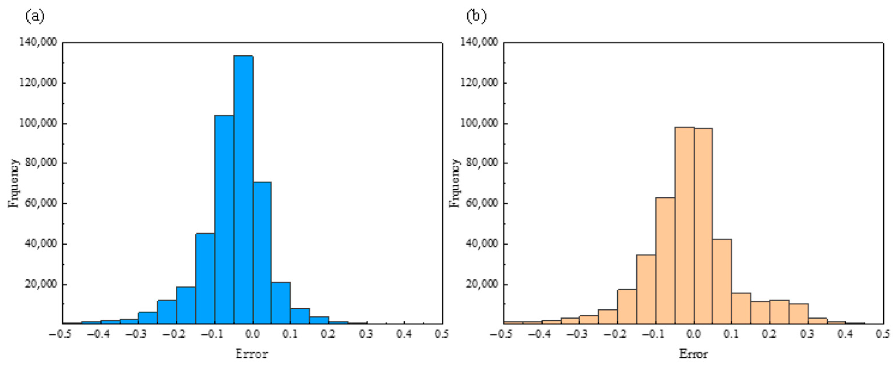
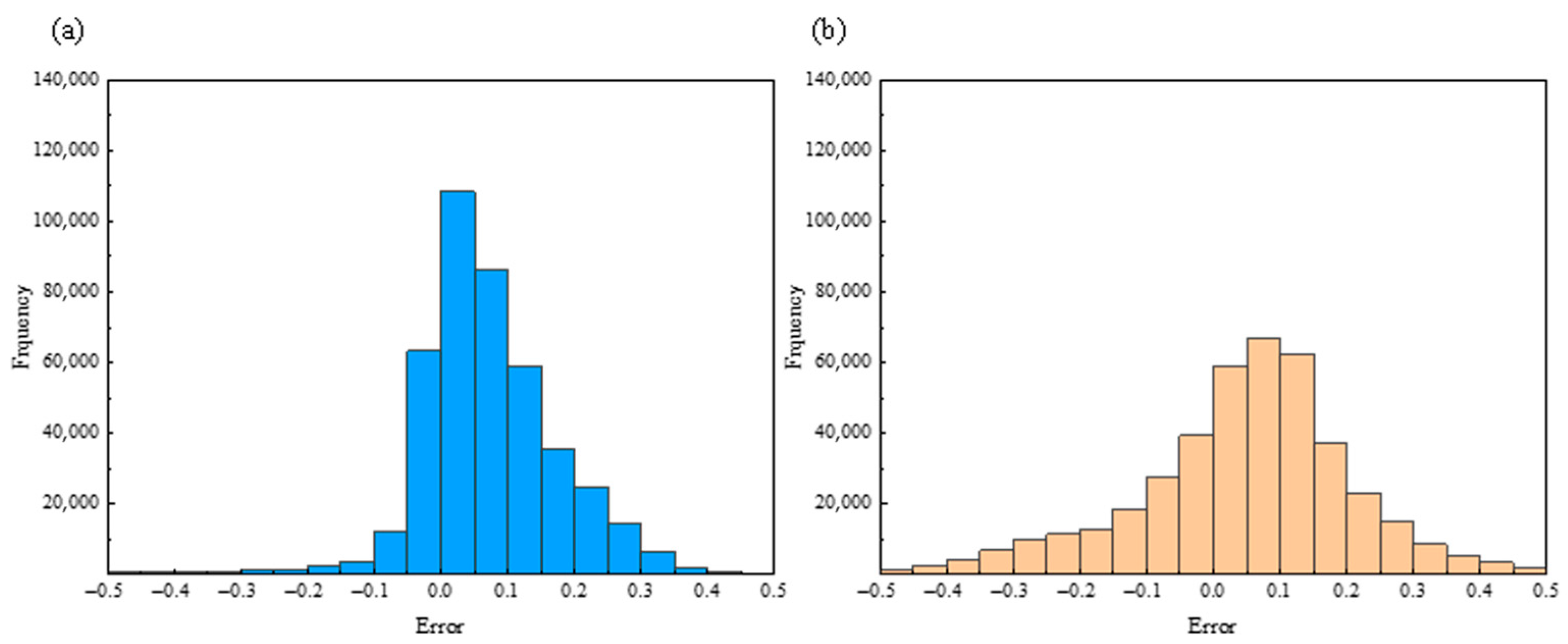
The relative errors of predicted air age using the two fast calculation methods are presented in Figure 6. It was observed that the distributions of the relative error approximate a normal distribution, with the majority of values concentrated within the range of −0.1 to 0.1, indicating that both methods provide good accuracy. As shown in Figure 6a, the error frequency of predicted air age based on the POD method decreases sharply as the relative error increases. And the distribution of the error frequency is asymmetrical, suggesting that the POD method is more prone to underpredicting the air age value. This may be attributed to the information loss during the downscaling process in the POD method. In contrast, Figure 6b shows a more symmetrical relative error distribution of the predicted air age from the ANN method.
The relative errors of predicted |PMV| using the two fast calculation methods are presented in Figure 7. The relative errors are larger than those of air age and predominantly concentrated within the range of −0.2 to 0.2, indicating that both methods provide relatively good accuracy. However, for poor predictions (outside the range of −0.2 to 0.2), the frequency of relative error for the ANN method is higher than that for the POD method, indicating that the POD method performs more accurate within the sampling range. However, this qualitative comparison alone is insufficient to determine which fast computation method is more suitable for subsequent optimization calculations. Therefore, the commonly used errors indicators are quantitatively calculated for the 15 cases, serving as evaluation metrics to identify the preferred method. We used three commonly used indicators to analyze the errors of POD and ANN, which are relative root mean square error (RRMSE), mean absolute error (MAE), and correlation coefficient (R2). The calculation formulas are shown in (16)–(18).
M A E = 1 N Σ i = 1 N | y ( i ) y p ( i ) |
R R M S E = 1 N Σ i = 1 N y ( i ) y p ( i ) 2 y ¯
R 2 = 1 Σ i = 1 N y ( i ) y p ( i ) 2 Σ i = 1 N y ( i ) y ¯
where N is the total number of datasets, y ( i ) is the output of simulated values, y p ( i ) is the output of model prediction, and y ¯ is the averaged value of the dataset. The model errors are shown in Table 3.
The optimization algorithm employed the fast calculation method to calculate the pareto frontier points, and its error primarily comes from the inaccuracy of the fast calculation method. Larger MAE or RRMSE values may result in erroneous optimization outcomes or convergence to a local optimum. A smaller R2 indicates that the fast calculation method fails to capture the key features, thereby undermining the reliability of the optimization algorithm. Therefore, a fast calculation method with lower MAE and RRMSE values and a higher R2 is required. From Table 3, we can see that POD performs better than ANN. This is mainly because the POD principle is to project the nonlinear problem of high latitudes into the space of low latitudes, and then interpolate, which can also solve the nonlinear problem well [17,41]. POD is a simple mathematical method, which only involves the operation of the matrix and the interpolation of the data. Therefore, the prediction within the sampling range will not have poor values, while the generalization problem of neural network cannot be avoided [42]. Even after full training, there may be a deviation from the performance of the prediction set for the ANN method. Therefore, the POD method was selected as the fast calculation method for the subsequent optimization process.

3.2. Comparison of Optimization Methods

In this study, the MOGA and Pareto search methods were used for optimization. For the MOGA, the population size is 50, the crossover fraction is 0.8, the mutation probability is 0.01, and the number of elite counts in the population is 2. Due to the differences in their solution mechanisms, different iterative convergence criteria were applied. The “spread” index was used as the MOGA convergence criterion. The defining equation is given by Equation (19):
s p r e a d = i = 1 M d i e + d i b + j = 1 n 1 d i j d ¯ d i e + d i b + n 1 d ¯
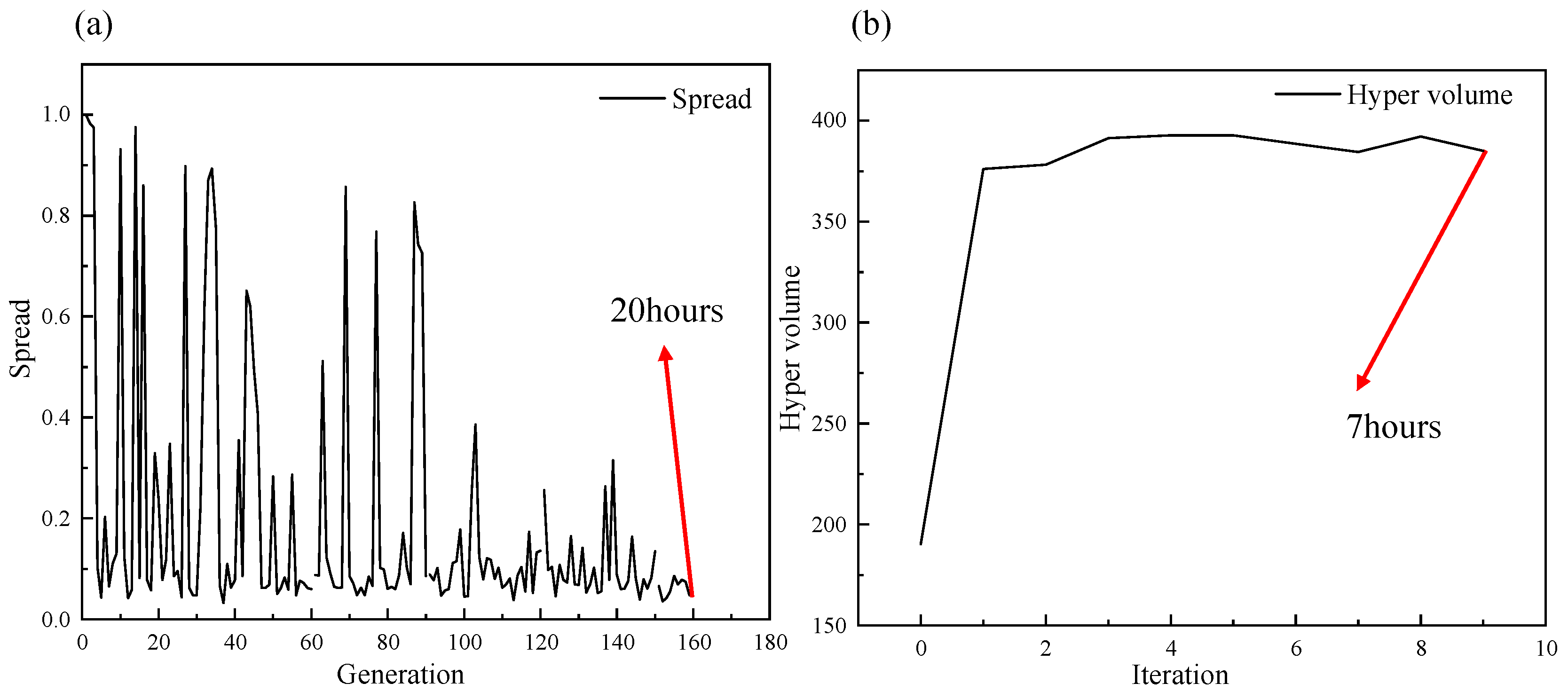
where M is the number of objective functions, n is the number of nondominated solutions, d i e and d i b are the distances of boundary solutions (extreme solutions in the objective space), respectively, d i j is the distance of neighboring solutions in the objective space, and d ¯ is the average value of all d i j . The spread index quantifies the spatial distribution of solutions in a multi-objective optimization algorithm. Generally, a smaller spread indicates a more uniform distribution of the solution set, while a larger spread signifies a more concentrated distribution. When the spread exhibits minimal variation, indicating that the distribution of the solution set found by the algorithm has stabilized, the algorithm can be considered to have converged. The MOGA method reached the stopping criterion at 162 generations (Figure 8a). Since the MOGA simulates the crossover and mutation of genes, which are inherently stochastic, the spread exhibits significant fluctuations in the early stages. As the number of generations increases, the spread gradually stabilizes and meets the convergence criterion after 162 generations.
The Pareto search algorithm adopts hypervolume as the iterative convergence criterion, and the hypervolume is defined as Equation (20):
H V S = V o l u m e i = 1 n R e c t a n g l e x i , r
where R e c t a n g l e x i , r denotes the rectangle (or hyper-rectangle) in multidimensional space determined by the solution x i and the reference point r . The hypervolume is a measure of the total volume occupied by the solution set in the objective space, indicating the total volume covered by the solution set. When the hypervolume stabilizes, it suggests that the solution has converged in the solution space. The Pareto search algorithm achieves the optimal solution after 9 iterations (Figure 8b). Since the Pareto search is a non-dominated sorting algorithm, each solution found in successive iterations is at least as good as the previous one. As a result, fewer iterations are needed to reach the convergence. However, because the Pareto search method requires non-dominated sorting at each iteration, it takes more time per iteration. Despite taking longer per iteration, the Pareto search method was more efficient in terms of overall computational cost due to its fewer iterations. In terms of computational cost, the MOGA took 20 h to complete, while the Pareto search algorithm required only 7 h.
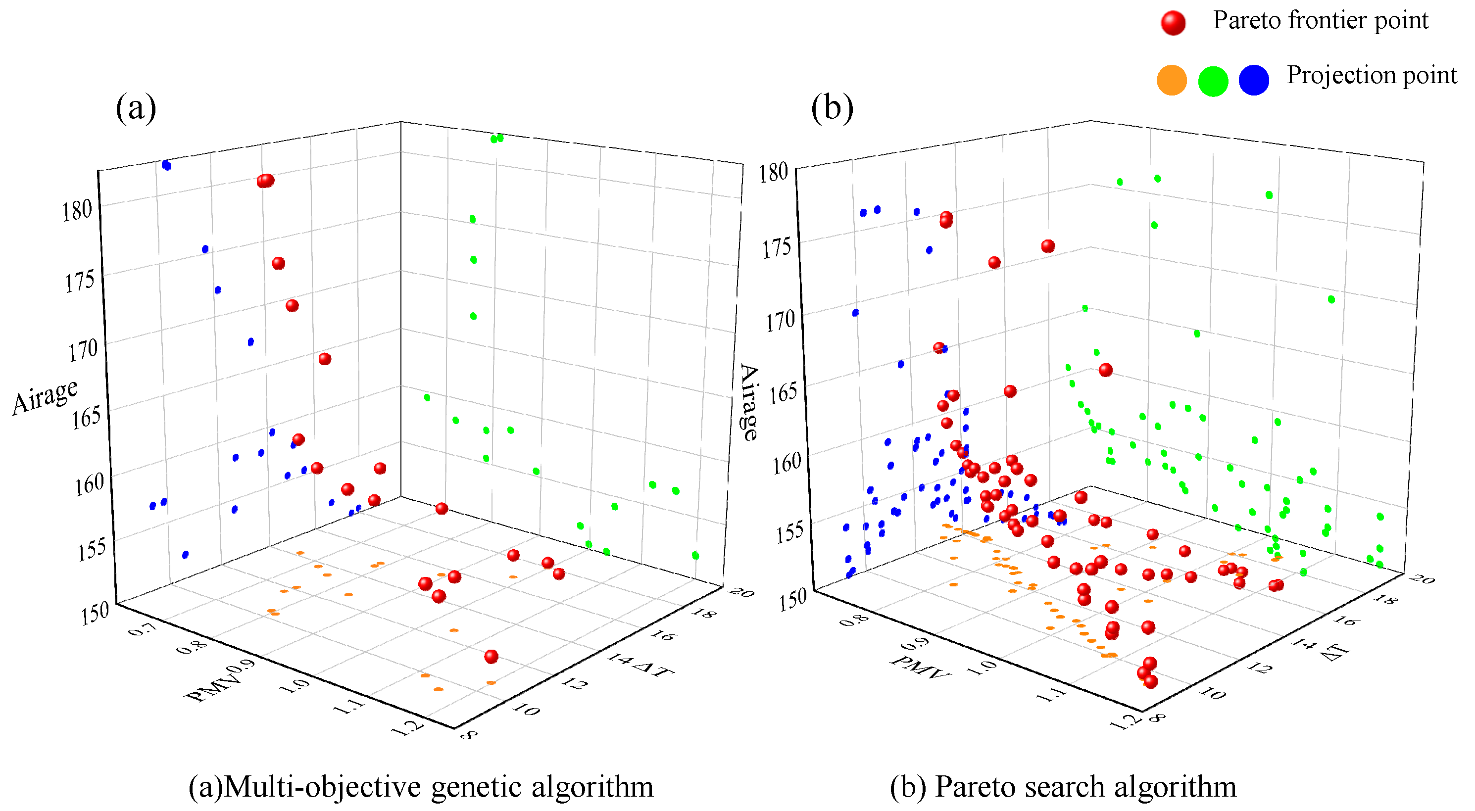
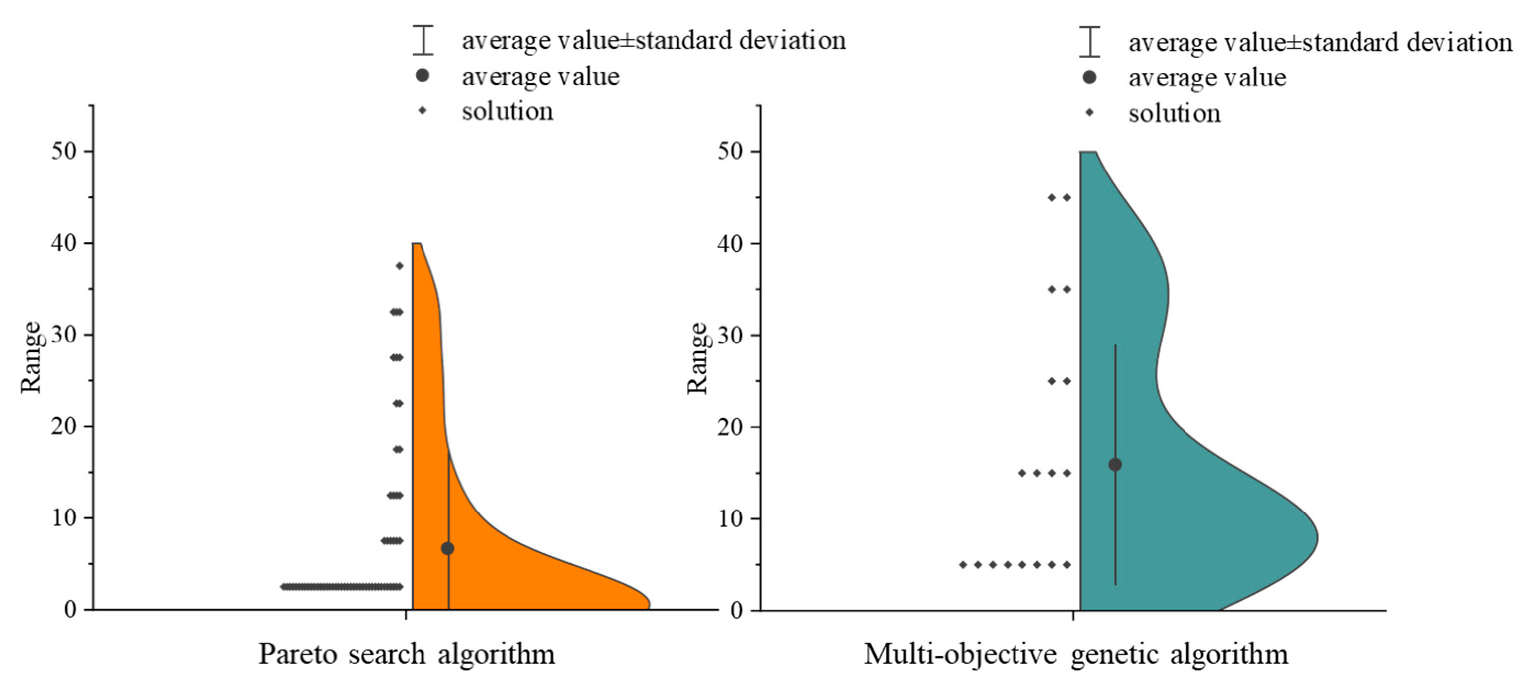
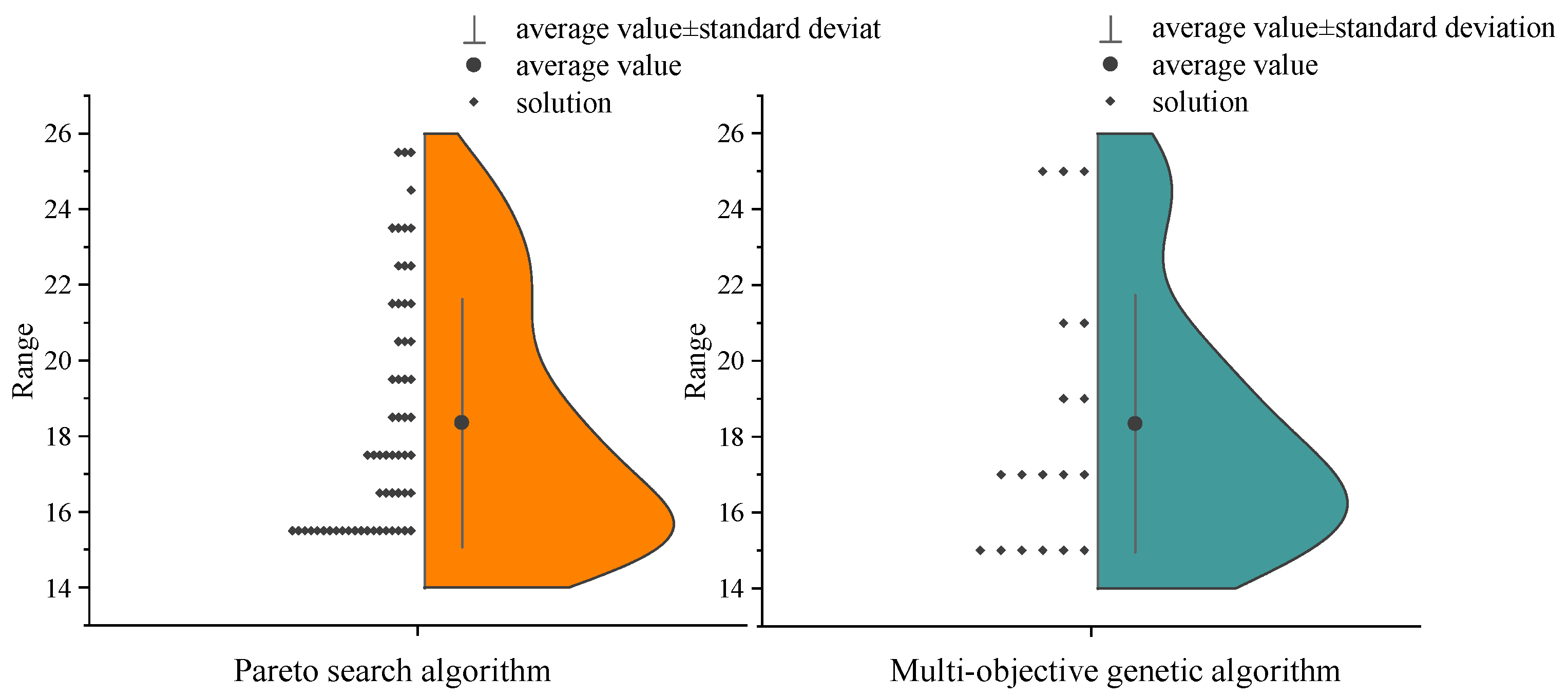
In addition to the computational time, the Pareto frontier distributions of MOGA and Pareto search methods are shown in Figure 9 for further analysis. As illustrated, the MOGA method identifies 18 Pareto frontier points, whereas the Pareto search algorithm identifies 60 points. The frontier point distributions of both algorithms are generally similar. However, the Pareto search algorithm identifies a broader set of solutions, offering more options for decision-making in subsequent steps. It also shows some deviation in specific regions when compared to the MOGA method. To further elucidate the distribution patterns, the Pareto frontier points of three design variables are presented as half-violin plots in Figure 10, Figure 11 and Figure 12.
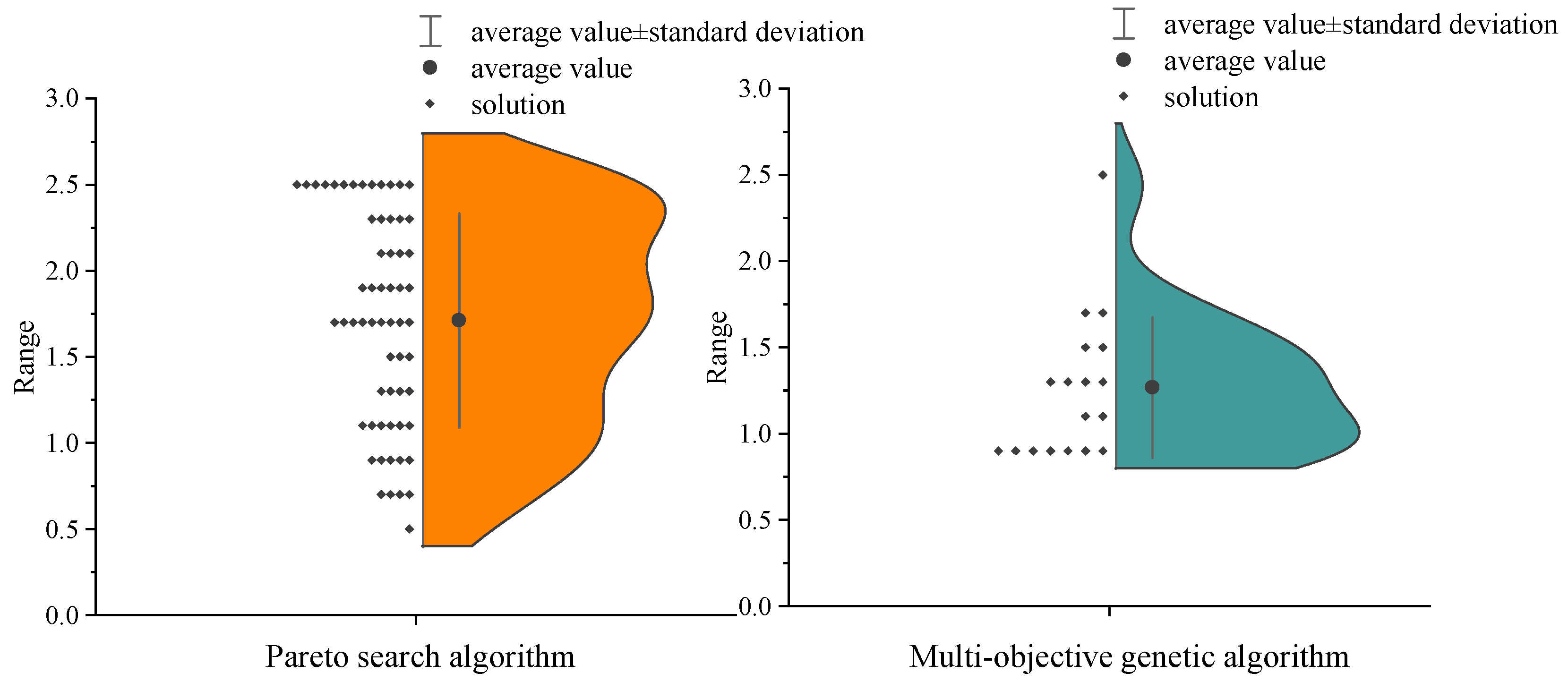
As shown in Figure 10, the distributions of solution sets obtained by the two optimization methods differ for air supply velocity. The Pareto search identifies solutions within the range of 0.5 to 2.5, with a more uniform distribution across this range. A uniform distribution offers a broader spectrum of choices for decision-makers, facilitating a more diversified approach to optimal solution selection. In contrast, the MOGA method identifies a solution set within the range of 1.0 to 2.5, with a more concentrated distribution in the range of 1.0 to 1.5. A more centralized distribution can provide clearer guidance to decision-makers, increasing the likelihood of identifying the optimal solution within the concentrated area. For the solution sets of the other two design variables—air supply angle and air supply temperature, the distributions from these two methods are similar. As shown in Figure 11, the solution set identified by the Pareto search algorithm is distributed within the range of 0 to 40, while the MOGA identifies solutions in the range of 0 to 50, indicating that the solution set from the Pareto search algorithm is more concentrated. Figure 12 shows that the ranges and distributions of solution sets from these two methods are nearly identical. Based on the above analysis, it is not possible to definitively conclude which method was more advantageous for this optimization problem. Therefore, we further analyze the optimal solutions from both methods in the next section.

3.3. Analysis of the Optimal Solutions

To identify the best optimal solution from the Pareto frontier points, this study assigned weight values to different optimization objectives. Two commonly used methods for assigning weights are the objective assignment and the subjective assignment methods. Given the inherent subjectivity in the latter, this study adopts the objective assignment method. Among objective assignment methods, the entropy weight method is particularly advantageous, as it mitigates bias introduced by human factors and offers a clearer rationale for the optimal solution.
The entropy weight method is based on the information entropy theory, in which the “entropy” is used to describe the degree of difference between variables in a system Through the entropy weighting method we can calculate the weight values corresponding to the three design variables of this study according to Equations (21)–(23) [43].
α = a 11 a 12 a 1 n a 21 a 22 a 2 n a m 1 a m 2 a m n
where α is the optimal solution matrix, where m is the number of optimal solutions and n is the number of design objectives.
β = b 11 b 12 b 1 n b 21 b 22 b 2 n b m 1 b m 2 b m n
β is the normalization matrix of α. β can be computed from the optimal solution matrix α. The formula is given in Equation (20).
b i j = a i j ( a i j ) m i n j ( a i j ) m a x j ( a i j ) m i n j
Since there are three design objectives for this study, j takes values from 1 to 3. The entropy weight of this matrix can then be calculated as follows Equations (24)–(26).
p i j = b i j / i = 1 m b i j
e j = 1 ln m i = 1 m p i j ln p i j
where e is the entropy value corresponding to the optimal solution matrix. Calculated according to the above formulas, we can get three entropy values corresponding to the three design objectives.
w j = ( 1 e j ) / j = 1 n ( 1 e j )
where is the weights correspond to the design objectives calculated by the entropy weighting method.
Based on the information entropy of the three design objectives, the weight values were calculated by the entropy weight method. The weight values of P M V , Δ T and air age are 0.282, 0.315 and 0.403, respectively, for the MOGA. The weight values are 0.263, 0.279 and 0.458 for the Pareto search algorithm. Finally, a comprehensive evaluation using the metric F was enabled. The definition of F is shown as follows:
F = w o 1 P M V M i n P M V M a x P M V M i n P M V + w o 2 Δ T M i n Δ T M a x Δ T M i n Δ T + w o 3 A i r   a g e M i n A i r   a g e M a x A i r   a g e M i n A i r   a g e
where w o 1 , w o 2 , w o 3 are the weight values of |PMV|, ΔT, and the air age, respectively. The Pareto search algorithm and MOGA are applied to Equation (24) to compute the score, such that the solution with the smallest F value is identified as the optimal solution. The details are shown in Table 4. The optimal solution calculated by the Pareto search algorithm is Optimal solution 1, and the optimal solution calculated by the MOGA is Optimal solution 2.
To validate the performances of the optimal solutions, we selected five random boundary conditions within the sampling range of the design variables (Table A2) and conducted a comprehensive comparison of the optimization objective values under the optimal solutions with those under the random boundary conditions.
Figure 13 compared the difference between the optimal solutions and the five random boundary conditions. The three axes represent the three optimization objectives. For the |PMV| value, Optimal solution 2 is the best performing among the seven cases, achieving a 40.3% improvement over the worst-performing Case 3 and a 9.5% improvement over the Case 4. Optimal solution 1 also performs better than the five random boundary conditions, with a 39.4% improvement over Case 3 and an 8.1% improvement over Case 4. Figure 14 provides a clearer comparison of the PMV distribution cloud maps across different scenarios. For the air age value, Optimal solution 1 outperforms the other cases, showing a 26% improvement over the worst-performing Case 2 and a 4.6% improvement over the Case 5. Optimal solution 2 also performs a 23.3% improvement over Case 2 and a 1.25% improvement over Case 5. Optimal solution 1 is superior to the Optimal solution 2. Figure 15 shows a clearer comparison of the air age distribution cloud maps. For the ΔT value, neither Optimal solution 1 nor Optimal solution 2 yields the best performance; both fall within the mid-range as shown in Figure 13. Overall, none of the optimal solutions achieves the best performance across all optimization objectives. Therefore, we need to select the optimal solution based on the specific requirements of the optimization objectives. If priority is given to the PMV performance, the Pareto search algorithm would be the preferred choice. Conversely, if the focus is on optimizing the air age and ΔT objectives, the MOGA should be selected.
The assignment problem in multi-objective optimization is inherently a decision-making challenge. In multi-objective optimization, a significant challenge lies in the difficulty of finding a set of optimal design variables that simultaneously achieve the optimal values for all design objectives. In practice, trade-offs and compromises must be made between conflicting objectives. These trade-offs can be approached subjectively, based on specific preferences, or through objective methods such as the entropy weight method. Additionally, it is crucial to consider the time and computational efficiency of the optimization process. Striking a balance between obtaining high-quality solutions and minimizing computational cost presents a further complexity in multi-objective optimization.

4. Discussion

4.1. Sensitivity Analysis

This study employs Sobol’s method to analyze the sensitivity of the model [44]. It utilizes analysis of variance (ANOVA) decomposition to compute specific-order sensitivity indices [45]. The specific formulas are shown in Equations (28)–(30).
V Y = V E Y | X i + E V Y | X i
where X i is a specific input target, Y is the output, V Y is the variance of the model, V E Y | X i is the main effect, which is also the first-order effect of X i on Y , and E V Y | X i is the residual term. We can calculate S i (First-Order Sensitivity Index) and S T i (Total-Effect Sensitivity Index) by Equations (29) and (30).
S i = V ( E ( Y X i ) ) V ( Y )
S T i = 1 V [ E ( Y X i ) ] V ( Y )
where X i is the matrix of all factors but X i .
I n t e r a c t i o n   E f f e c t = S T i S i
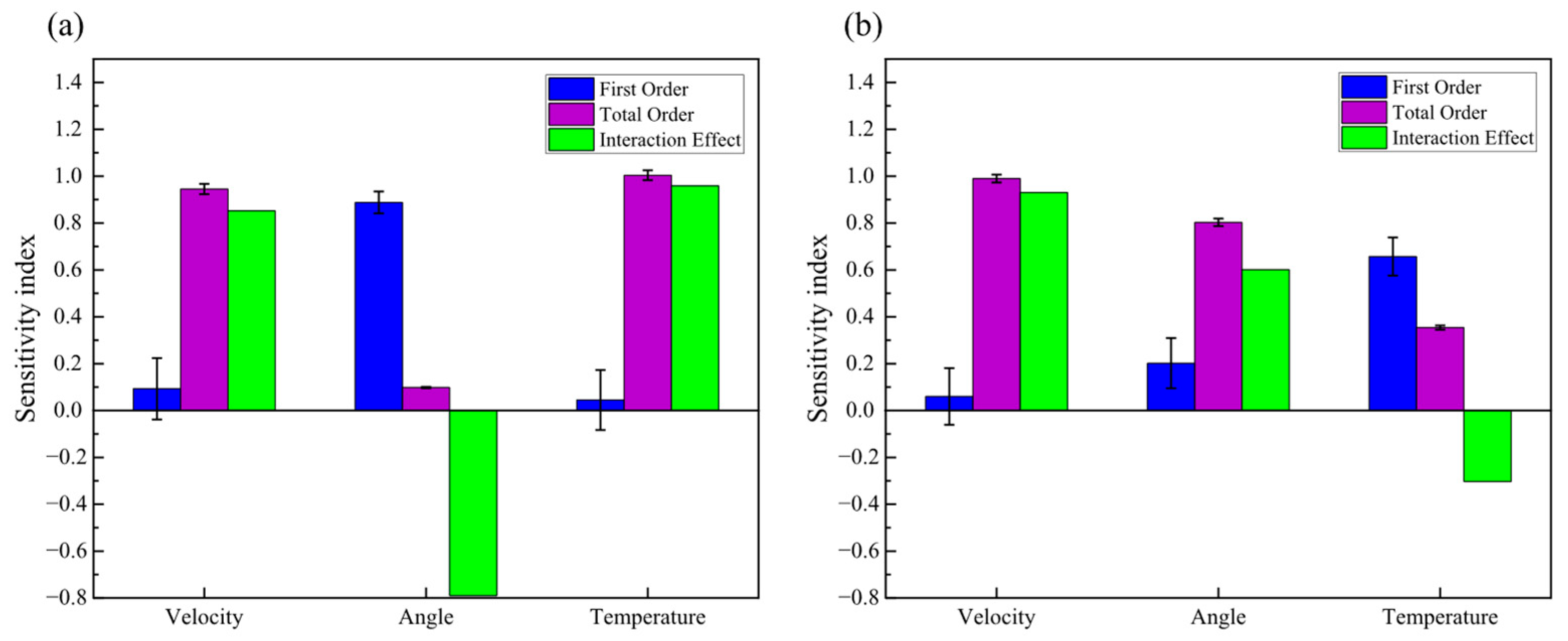
I n t e r a c t i o n   E f f e c t shows the interaction effect between the parameters. A positive interaction suggests a mutual enhancement, whereas a negative interaction implies a mutual offset.
In this study, QMC (Quasi-Monte Carlo) sampling methods [46] were used to perform sensitivity analysis and uncertainty analysis with 10,000 samples in the range of three design parameters. Then we use POD models for rapid calculation and then conduct sensitivity analysis.
In Figure 16, the first-order index reflects the direct influence of a parameter on the output, the total-order index represents the combined effect of this parameter with other parameters, and the interaction effect quantifies the strength of such coupling. From Figure 16a, the first-order index of the angle for the POD model is larger than that of temperature and velocity, indicating that air age is primarily affected by the angle. In contrast, Figure 16b shows that temperature exerts a greater influence on PMV. Furthermore, in Figure 16a, the total-order indices and interaction effects of velocity and temperature are both high, suggesting that their influence on air age is mainly achieved through coupling with the angle. This implies that the effects of velocity and temperature on air age are more pronounced at certain angles, whereas the influence of angle on air age remains substantial across different velocities and temperatures. Similarly, in Figure 16b, the first-order indices of velocity and angle for PMV are relatively low, but their total-order indices are high, indicating that their effects on PMV become significant under certain temperature conditions. This is consistent with practical knowledge, as higher temperatures amplify the improvement in thermal comfort brought by increased wind speed.

4.2. Practical Implications

In this study, an optimization framework is proposed for the design of ventilation systems in supersonic passenger aircraft. Prior to the practical application of such aircraft, this framework can be used to optimize the air supply system in advance. The optimized parameters can ensure passenger thermal comfort, maintain air freshness in the breathing zone, and improve the energy efficiency of the cabin ventilation system. The framework consists of a rapid computation module and an optimization module, and its application is not limited to the ventilation system of supersonic aircraft. It can also be extended to solve other optimization problems and has the potential to be applied in various fields. Furthermore, the code developed in this study is self-written, allowing for easy modification, adaptation, and integration with other models. In the future, it has potential for integration with other software platforms to address real-world engineering challenges.

4.3. Limitations and Future Prospects

This study proposes a framework for the rapid calculation and optimization of ventilation systems in supersonic passenger aircraft. However, only three design variables are considered: air supply velocity, air supply temperature, and air supply angle. This framework is specifically applicable to cabin environments with the ventilation layout and geometric configuration used in this study, where these three parameters are sufficient to determine key indicators such as thermal comfort and air freshness. If different ventilation modes are adopted, the number and location of air supply outlets will vary. In such cases, additional geometric factors, including the number and position of the diffusers, must be taken into account, and the model would require retraining. Moreover, the proposed methods and conclusions need to be validated through experiments conducted in actual supersonic aircraft cabins, which may serve as a future research direction.

5. Conclusions

In this study, a multi-objective optimization approach was applied to determine the optimal supply air parameters in a supersonic aircraft cabin. The optimization objectives were PMV, the air age and temperature difference between supply and exhaust air, with supply air velocity, temperature and supply air angle as the design variables. The fast calculation methods were employed to calculate the optimization objectives within the ranges of design variables, and the multi-objective optimization methods were utilized to identify optimal solutions. The key findings are summarized as follows:
(1) A comparison was conducted between the POD method and ANN method. The POD method yielded lower RRMSEs for PMV (0.0647) and air age (0.0315), compared to ANN’s errors of 0.180 and 0.124, respectively. Thus, the POD method was selected as the fast calculation method due to its superior accuracy;
(2) The MOGA found 18 Pareto frontier points with a total computation time of 20 h. In contrast, the Pareto search algorithm found 60 Pareto frontier points in just 7 h, demonstrating a more efficient computation process and offering a broader solution space for decision-making;
(3) The entropy weight method was used to determine the final optimal solution. The weights assigned to PMV, ΔT, and air age were 0.282, 0.315, and 0.423 for the Pareto search algorithm, and 0.263, 0.279, and 0.458 for the MOGA, respectively. However, it should be noted that neither of these algorithms can achieve optimal performance across all objectives. Therefore, the optimal solution should be selected according to the specific requirements of the optimization objectives, and the time and computational efficiency of the optimization process should also be considered.

Author Contributions

Conceptualization, F.L. and X.C.; methodology, F.L. and G.Y.; validation, S.N.; resources, X.C. and Z.H.; writing—original draft preparation, G.Y.; writing—review and editing, F.L. and X.C.; visualization, S.N.; supervision, F.L. and Y.W. All authors have read and agreed to the published version of the manuscript.

Funding

This research was financially supported by Jiangsu Province Science and Technology Program Funds (Frontier Technology R&D Program) (No. BF2024057) and the Postgraduate Research &Practice Innovation Program of Jiangsu Province (No. SJCX25_0612).

Institutional Review Board Statement

Not applicable.

Informed Consent Statement

Not applicable.

Data Availability Statement

The data that supports the findings of this study is available from the corresponding author upon reasonable request. The data are not publicly available due to privacy or ethical restrictions.

Conflicts of Interest

The authors declare no conflicts of interest.

Abbreviation

Nomenclature
S Momentum sourcekg/(m2·s2)
A s Superficial area of the diffuserm2
U s Superficial velocity of the diffuserm/s
U r e a l Real velocity of the diffuserm/s
V c e l l Volume of momentum source cellsm3
q l Heat flow rate per unit lengthW/m
t 1 ,  t 2 Inner/outer wall temperature°C
t i n Indoor temperature°C
λ i Thermal conductivity of the i-th insulation layerW/(m·K)
r i Distance from the center for the i-th layerm
h 1 Convective heat transfer coefficient (inner wall)W/(m2·K)
τ ¯ Averaged air ages
c i ( t ) Tracer gas concentration at time tppm
P M V Predicted Mean Vote
Δ T Temperature difference between exhaust and supply air°C
U Airflow velocity matrix
φ i Spatial mode
λ Eigenvalue
v Eigenvector
E P Energy contribution of the first P eigenvalues%
b i Projection of velocity field onto the ith spatial mode
U ¯ Row-averaged velocity
Y i Target output
y i Predicted output
O 1 Objective 1: Minimize |PMV|
O 2 Objective   2 : Minimize   τ ¯
O 3 Objective   3 : Minimize   Δ T
T Supply air temperature°C
ν Supply air velocitym/s
θ Supply air angle°
M A E Mean absolute error
R R M S E Relative root mean square error
R 2 Coefficient of determination
α Optimal solution matrix
β Normalized matrix
w j Weight for the j-th objective
F Comprehensive evaluation metric
S i First-order sensitivity index
S T i Total-effect sensitivity index

Appendix A

Table A1. 15 random selected boundary conditions for the validation of fast calculation methods.
Supply Air Temperature (°C)Supply Air Angle (°)Supply Air Velocity (m/s)
21340.48
15510.67
16440.54
24350.63
20150.3
23401.66
1750.85
21381.44
21401.8
15441.35
21531.43
19591.22
15460.49
20351.33
17562.16
Table A2. Random selected boundary conditions for optimal solution comparison.
Case NumberSupply Air Temperature (°C)Supply Air Angle (°)Supply Air Velocity (m/s)
Case121340.48
Case217562.16
Case323401.66
Case415441.35
Case520150.3

References

  1. He, J.; Pan, R.; Cheng, W.; Guo, C.; Meng, Z. Competitiveness Evaluation Method of Supersonic Civil Aircraft Based on Analytic Hierarchy Process. Aerospace 2025, 12, 37. [Google Scholar] [CrossRef]
  2. The World of Air Transport in 2020. Available online: https://www2023.icao.int/annual-report-2020/Pages/the-world-of-air-transport-in-2020_zh.aspx (accessed on 20 August 2025).
  3. Teleszewski, T.J.; Gładyszewska-Fiedoruk, K. Development of a Simplified One-Dimensional Model of Humidity in the Cabin of a Passenger Aircraft Based on an Experiment. Atmosphere 2025, 16, 280. [Google Scholar] [CrossRef]
  4. Mariita, R.M.; Davis, J.H.; Lottridge, M.M.; Randive, R.V.; Witting, H.; Yu, J. Towards a Healthy Car: UVC LEDs in an Automobile’s HVAC Demonstrates Effective Disinfection of Cabin Air. Atmosphere 2022, 13, 1926. [Google Scholar] [CrossRef]
  5. Hyper Mach Unveils Sonicstar Supersonic Business Jet Concept. Available online: https://newatlas.com/hypermach-sonicstar-ssbj-concept/18974/ (accessed on 20 August 2025).
  6. Boom Supersonic Announces Significant Overture Program Advances. Available online: https://boomsupersonic.com/press-release/boom-supersonic-announces-significant-overture-program-advances (accessed on 20 August 2025).
  7. Zhai, Z.J.; Xue, Y.; Chen, Q. Inverse design methods for indoor ventilation systems using CFD-based multi-objective genetic algorithm. Build. Simul. 2014, 7, 661–669. [Google Scholar] [CrossRef]
  8. Xue, Y.; Liu, W.; Wang, Q.; Bu, F. Development of an integrated approach for the inverse design of built environment by a fast fluid dynamics-based generic algorithm. Build. Environ. 2019, 160, 106205. [Google Scholar] [CrossRef]
  9. Zhang, T.-H.; You, X.-Y. A simulation-based inverse design of preset aircraft cabin environment. Build. Environ. 2014, 82, 20–26. [Google Scholar] [CrossRef]
  10. Bjelić, M.B.; Radičević, B.S.; Kovanda, K.; Kolařík, L.; Petrović, A.V. Multi-objective calibration of the double-ellipsoid heat source model for GMAW process simulation. Therm. Sci. 2021, 26, 2081–2092. [Google Scholar] [CrossRef]
  11. Al-Ghussain, L.; Abubaker, A.M.; Ahmad, A.D. Superposition of Renewable-Energy Supply from Multiple Sites Maximizes Demand-Matching: Towards 100% Renewable Grids in 2050. Appl. Energy 2021, 284, 116402. [Google Scholar] [CrossRef]
  12. Liu, W.; Duan, R.; Chen, C.; Lin, C.-H.; Chen, Q. Inverse design of the thermal environment in an airliner cabin by use of the CFD-based adjoint method. Energy Build. 2015, 104, 147–155. [Google Scholar] [CrossRef]
  13. Liu, W.; You, R.; Zhang, J.; Chen, Q. Development of a fast fluid dynamics-based adjoint method for the inverse design of indoor environments. J. Build. Perform. Simul. 2017, 10, 326–343. [Google Scholar] [CrossRef]
  14. Zhao, X.; Liu, W.; Lai, D.; Chen, Q. Optimal design of an indoor environment by the CFD-based adjoint method with area-constrained topology and cluster analysis. Build. Environ. 2018, 138, 171–180. [Google Scholar] [CrossRef]
  15. Zhao, M.; Liang, L.; Long, Z. Optimization of the vents in the airliner cockpit for uniform air supply based on the adjoint method and genetic algorithm. Build. Environ. 2025, 278, 112962. [Google Scholar] [CrossRef]
  16. Xu, Y.; Wei, X.; Xia, Y.; Yu, Y.; Zeng, L.; Cao, G.; Gao, J. Prompt design of direction air supply using CFD-based proper orthogonal decomposition method considering locally dense sample distribution. Build. Environ. 2023, 244, 110812. [Google Scholar] [CrossRef]
  17. Wei, Y.; Zhang, T.; Jin, H. Rapid prediction of airborne gaseous pollutant transport in aircraft cabins based on proper orthogonal decomposition and the Markov chain method. Build. Environ. 2023, 228, 109816. [Google Scholar] [CrossRef]
  18. Liang, L.; Zhao, M.; Wang, Y.; Long, Z.; Yin, H. Optimization of indoor thermal environment for high-altitude sentry buildings with attached ventilation based on proper orthogonal decomposition. Build. Environ. 2025, 267, 112200. [Google Scholar] [CrossRef]
  19. Lu, Y.; Wang, T.; Zhao, C.; Zhu, Y.; Jia, X.; Zhang, L.; Shi, F.; Jiang, C. An efficient design method of indoor ventilation parameters for high-speed trains using improved proper orthogonal decomposition reconstruction. J. Build. Eng. 2023, 71, 106600. [Google Scholar] [CrossRef]
  20. Wei, C.; Ooka, R. Indoor airflow field reconstruction using physics-informed neural network. Build. Environ. 2023, 242, 110563. [Google Scholar] [CrossRef]
  21. Zhang, T.; Li, X.; Zhao, Q.; Rao, Y. Control of a novel synthetical index for the local indoor air quality by the artificial neural network and genetic algorithm. Sustain. Cities Soc. 2019, 51, 101714. [Google Scholar] [CrossRef]
  22. Zhao, D.; You, X.-Y. Inverse design optimisation of a novel range hood based on intelligent algorithms and computational fluid dynamics simulations. Adv. Powder Technol. 2020, 31, 730–745. [Google Scholar] [CrossRef]
  23. Wang, C.; Hu, K.; Liu, Y. Multi-objective optimization of supply air inlet structure for impinging jet ventilation system based on radial basis function neural network. Case Stud. Therm. Eng. 2025, 65, 105629. [Google Scholar] [CrossRef]
  24. Design and Analysis of a Supersonic Business Jet. Available online: https://www.sjsu.edu/ae/docs/project-thesis/Harshil.Hitesh.Patel.F18.pdfv (accessed on 20 August 2025).
  25. Ahmadzadeh, M.; Farokhi, E.; Shams, M. Investigating the effect of air conditioning on the distribution and transmission of COVID-19 virus particles. J. Clean. Prod. 2021, 316, 128147. [Google Scholar] [CrossRef]
  26. Hu, X.; You, X.-Y. Determination of the optimal control parameter range of air supply in an aircraft cabin. Build. Simul. 2015, 8, 465–476. [Google Scholar] [CrossRef]
  27. Deng, B.; Wang, J.; Tang, J.; Gao, J. Improvement of the momentum method as the diffuser boundary condition in CFD simulation of indoor airflow: Discretization viewpoint. Build. Environ. 2018, 141, 55–60. [Google Scholar] [CrossRef]
  28. Concorde Airframe Materials. Available online: www.heritageconcorde.com/airframe-materials (accessed on 20 August 2025).
  29. Zhang, T.; Dong, J.; Liu, S. Modeling and Measuring the Leaked-Air Rate into the Insulation Layer of a Single-Aisle Aircraft Cabin. Buildings 2022, 12, 652. [Google Scholar] [CrossRef]
  30. Martinho, N.; Lopes, A.; da Silva, M.G. Evaluation of errors on the CFD computation of air flow and heat transfer around the human body. Build. Environ. 2012, 58, 58–69. [Google Scholar] [CrossRef]
  31. Li, J.; Cao, X.; Liu, J.; Wang, C.; Zhang, Y. Global airflow field distribution in a cabin mock-up measured via large-scale 2D-PIV. Build. Environ. 2015, 93, 234–244. [Google Scholar] [CrossRef]
  32. Li, F.; Liu, J.; Ren, J.; Cao, X. Predicting contaminant dispersion using modified turbulent Schmidt numbers from different vortex structures. Build. Environ. 2018, 130, 120–127. [Google Scholar] [CrossRef]
  33. Reiss, J.; Schulze, P.; Sesterhenn, J.; Mehrmann, V. The Shifted Proper Orthogonal Decomposition: A Mode Decomposition for Multiple Transport Phenomena. SIAM J. Sci. Comput. 2015, 40, A1322–A1344. [Google Scholar] [CrossRef]
  34. Wu, Y.-C.; Feng, J.-W. Development and Application of Artificial Neural Network. Wirel. Pers. Commun. 2018, 102, 1645–1656. [Google Scholar] [CrossRef]
  35. Deb, K. Multi-objective Genetic Algorithms: Problem Difficulties and Construction of Test Problems. Evol. Comput. 1999, 7, 205–230. [Google Scholar] [CrossRef]
  36. Li, N.; Yang, L.; Li, X.D.; Li, X.; Tu, J.; Cheung, S.C. Multi-objective optimization for designing of high-speed train cabin ventilation system using particle swarm optimization and multi-fidelity Kriging. Build. Environ. 2019, 155, 161–174. [Google Scholar] [CrossRef]
  37. Fanger, P.O. Calculation of Thermal Comfort, Introduction of a Basic Comfort Equation. ASHRAE Trans. 1967, 73, III4.1–III4.20. [Google Scholar]
  38. Yu, C.-Y.; Lin, C.-H.; Yang, Y.-H. Human body surface area database and estimation formula. Burns 2010, 36, 616–629. [Google Scholar] [CrossRef] [PubMed]
  39. Jones, B. Air Quality Within Commercial Aircraft; ASHRAE IAQ Applications: Norcross, GA, USA, 2008; p. 9. [Google Scholar]
  40. Wang, J.H.; Zhang, T.F.; Zhou, H.B.; Wang, S. Inverse design of aircraft cabin environment using computational fluid dynamics-based proper orthogonal decomposition method. Indoor Built Environ. 2018, 27, 1379–1391. [Google Scholar] [CrossRef]
  41. Tallet, A.; Allery, C.; Allard, F. POD approach to determine in real-time the temperature distribution in a cavity. Build. Environ. 2015, 93, 34–49. [Google Scholar] [CrossRef]
  42. Zhang, T.; Zhao, C.; Chen, G.; Jiang, Y.; Chen, F. Feature contamination: Neural networks learn uncorrelated features and fail to generalize. arXiv 2024, arXiv:2406.03345. [Google Scholar] [CrossRef]
  43. Li, Z.; Luo, Z.; Wang, Y.; Fan, G.; Zhang, J. Suitability evaluation system for the shallow geothermal energy implementation in region by Entropy Weight Method and TOPSIS method. Renew. Energy 2022, 184, 564–576. [Google Scholar] [CrossRef]
  44. Sobol, I. On sensitivity estimation for nonlinear mathematical models. Mater. Model. 1990, 2, 112–118. [Google Scholar]
  45. Hamdia, K.M.; Ghasemi, H.; Zhuang, X.; Alajlan, N.; Rabczuk, T. Sensitivity and uncertainty analysis for flexoelectric nanostructures. Comput. Methods Appl. Mech. Eng. 2018, 337, 95–109. [Google Scholar] [CrossRef]
  46. Guo, D.; Wang, X. Quasi-Monte Carlo filtering in nonlinear dynamic systems. IEEE Trans. Signal Process. 2006, 54, 2087–2098. [Google Scholar] [CrossRef]
Figure 1. New generation of the supersonic aircraft: (a) SonicStar supersonic business jet concept [5], (b) Overture from Boom Supersonic [6].
Atmosphere 16 01005 g001
Figure 2. Multi-objective optimization framework of the supply air parameters in a supersonic aircraft cabin.
Atmosphere 16 01005 g002
Figure 3. Front view of the cabin: (a) Supersonic cabin structure, (b) Manikin Structure.
Atmosphere 16 01005 g003
Figure 4. Grid independence analysis.
Atmosphere 16 01005 g004
Figure 5. (a) Measured section in the aircraft cabin, (b) Comparison of PIV experimental velocity data with the predicted velocity [32].
Atmosphere 16 01005 g005
Figure 6. Relative errors of the air age for two fast calculation methods: (a) Air age prediction based on the POD method, (b) Air age prediction based on the ANN method.
Atmosphere 16 01005 g006
Figure 7. Relative errors of the |PMV| for two fast calculation methods: (a) |PMV| prediction based on the POD method, (b) |PMV| prediction based on the ANN method.
Atmosphere 16 01005 g007
Figure 8. Algorithm iteration convergence for (a) MOGA and (b) Pareto search algorithm. (Spread indicates the uniformity of the distribution of the solution set in space, and Hypervolume indicates the hypervolume of the solution space occupied by the solution set in space).
Atmosphere 16 01005 g008
Figure 9. Pareto frontier distributions for (a) MOGA, (b) Pareto search algorithm.
Atmosphere 16 01005 g009
Figure 10. Pareto frontier distributions of air supply velocity for two optimization methods.
Atmosphere 16 01005 g010
Figure 11. Pareto frontier distributions of air supply angle for two optimization methods.
Atmosphere 16 01005 g011
Figure 12. Pareto frontier distributions of air supply temperature for two optimization methods.
Atmosphere 16 01005 g012
Figure 13. Comparison of the optimal solutions with the random design variables.
Atmosphere 16 01005 g013
Figure 14. PMV comparison of the optimal solutions with Case 3 and Case 4.
Atmosphere 16 01005 g014
Figure 15. The air age comparison of the optimal solutions with Case 2 and Case 5.
Atmosphere 16 01005 g015
Figure 16. Sensitivity analysis of POD model for (a) Air age, (b) PMV.
Atmosphere 16 01005 g016
Table 1. Boundary conditions for the CFD simulation.
Boundary ParametersSettingsValues
Wall (left and right)Constant temperature40 °C
Wall (other)Constant heat flux0
Air supply diffusersVelocity-inlet
Air exhaustPressure outlet
SeatConstant heat flux0
Table 2. Sampling ranges of different design variables.
Design VariableMinimumMaximumNumber of Samples
Supply Air Velocity0.2 m/s2.5 m/s4
Supply Air Temperature15 °C25 °C3
Supply Air Angle60°4
Table 3. Errors of the POD and ANN models.
ModelObjectiveMAERRMSER2
PODAir age0.01740.03150.957
|PMV|0.03020.06470.911
ANNAir age0.1130.1240.759
|PMV|0.1980.1800.733
Table 4. Optimization objectives and design variables for the optimal solutions.
Optimization ObjectivesDesign Variables
|PMV|ΔT (K)Air Age (s)Supply Air velocity (m/s)Supply Air Temperature (°C)Supply Air Angle
Optimal solution 10.7314.27152.592.5015
Optimal solution 20.7213.73158.091.6813.215.9°
Disclaimer/Publisher’s Note: The statements, opinions and data contained in all publications are solely those of the individual author(s) and contributor(s) and not of MDPI and/or the editor(s). MDPI and/or the editor(s) disclaim responsibility for any injury to people or property resulting from any ideas, methods, instructions or products referred to in the content.