Article

A Hybrid Air Quality Prediction Model Integrating KL-PV-CBGRU: Case Studies of Shijiazhuang and Beijing

1
School of Remote Sensing and Information Engineering, North China Institute of Aerospace Engineering, Langfang 065000, China
2
Hebei Province Key Laboratory of Intelligent Processing of Remote Sensing Data and Target Analysis, Langfang 065000, China
3
High-Resolution Earth Observation System-Hebei Data and Application Center, Shijiazhuang 050000, China
4
Digital Space Technology Co., Langfang 065000, China
*
Author to whom correspondence should be addressed.
Atmosphere 2025, 16(8), 965; https://doi.org/10.3390/atmos16080965 (registering DOI)
Submission received: 19 June 2025 / Revised: 22 July 2025 / Accepted: 29 July 2025 / Published: 15 August 2025
(This article belongs to the Section Atmospheric Techniques, Instruments, and Modeling)

Abstract

Accurate prediction of the Air Quality Index (AQI) is crucial for protecting public health; however, the inherent instability and high volatility of AQI present significant challenges. To address this, the present study introduces a novel hybrid deep learning model, KL-PV-CBGRU, which utilizes Kalman filtering to decompose AQI data into features and residuals, effectively mitigating volatility at the initial stage. For residual components that continue to exhibit substantial fluctuations, a secondary decomposition is conducted using variational mode decomposition (VMD), further optimized by the particle swarm optimization (PSO) algorithm to enhance stability. To overcome the limited predictive capabilities of single models, this hybrid framework integrates bidirectional gated recurrent units (BiGRU) with convolutional neural networks (CNNs) and convolutional attention modules, thereby improving prediction accuracy and feature fusion. Experimental results demonstrate the superior performance of KL-PV-CBGRU, achieving R2 values of 0.993, 0.963, 0.935, and 0.940 and corresponding MAE values of 2.397, 8.668, 11.001, and 14.035 at 1 h, 8 h, 16 h, and 24 h intervals, respectively, in Shijiazhuang—surpassing all benchmark models. Ablation studies further confirm the critical roles of both the secondary decomposition process and the hybrid architecture in enhancing predictive accuracy. Additionally, comparative experiments conducted in Beijing validate the model’s strong transferability and consistent outperformance over competing models, highlighting its robust generalization capability. These findings underscore the potential of the KL-PV-CBGRU model as a powerful and reliable tool for air quality forecasting across varied urban settings.

1. Introduction

With the acceleration of urbanization, pollution sources such as industrial emissions, traffic exhaust, and construction dust are increasing, leading to deteriorating air quality that threatens public health and causes economic losses [1]. Studies have shown that high concentrations of pollutants like PM2.5, nitrogen dioxide (NO2), and ozone (O3) can lead to both acute and chronic conditions, including respiratory illnesses, cardiovascular problems, and asthma, with particularly severe effects on children, the elderly, and individuals with pre-existing health conditions [2,3]. Long-term exposure to polluted environments also increases the risk of cancer [4]. The Air Quality Index (AQI) is a standardized indicator used to measure and report the severity of air pollution by converting the concentrations of major pollutants into a single value that visually reflects air quality [5]. The AQI commonly includes measurements of fine particulate matter (PM2.5), inhalable particulate matter (PM10), sulfur dioxide (SO2), NO2, O3, and carbon monoxide (CO). It is typically categorized into six levels: 0–50 (excellent), 51–100 (good), 101–150 (mild pollution), 151–200 (moderate pollution), 201–300 (severe pollution), and 300+ (extremely severe pollution), with higher values indicating greater health risks. As a result, research into AQI prediction and the analysis of its influencing factors holds substantial significance for protecting public health and promoting the sustainable development of air quality. Traditional AQI forecasting approaches are generally classified into physical–chemical models and statistical models. Physical–chemical models rely on principles such as atmospheric dynamics, chemical reactions, and pollutant transport, using simulation to predict the generation, diffusion, and transformation of pollutants in the atmosphere. Wyat et al. [6], based on the CMAQ model, simulated air quality and evaluated its performance using different versions of the model; however, physical–chemical models generally require extensive data inputs, and their modeling processes are often complex and computationally intensive. Statistical models, including the Autoregressive Integrated Moving Average Model (ARIMA), Grey Model (GM), and multiple linear regression, rely on historical data to forecast air quality by analyzing statistical relationships between AQI and factors such as meteorological conditions and pollutant emissions [7,8,9]; however, due to the highly nonlinear and unstable nature of AQI data, these models often struggle to deliver accurate predictions. In recent years, artificial intelligence (AI) methods have developed rapidly and, compared with traditional approaches, offer stronger nonlinear modeling capabilities, demonstrating superior performance in both cross-regional and cross-temporal AQI predictions. As a result, AI techniques have become widely used in AQI forecasting and now represent a major research focus in the field [10,11,12]. Currently, machine learning and deep learning approaches to AQI prediction generally fall into two categories: standalone deep learning models and those combining time series decomposition algorithms with deep learning architectures. Standalone models may use a single algorithm paired with optimization techniques; for instance, Su et al. [13] applied a backpropagation (BP) neural network optimized via genetic algorithms to predict AQI at six monitoring stations in Dalian. Maleki et al. [14] constructed datasets combining meteorological variables and varying time steps to enable hourly AQI forecasting in Ahvaz, Iran, using an artificial neural network (ANN). Kumar et al. [15] used a bidirectional gated recurrent unit (BiGRU) model with seven time steps to predict daily AQI data across four locations in Bangladesh, while Kumar et al. [16] employed a decision tree (DT) model enhanced with grey wolf optimization (GWO) to improve AQI prediction accuracy for major Indian cities. Despite their strengths, individual neural networks often face limitations in generalization, prompting researchers to develop hybrid models that leverage the strengths of multiple algorithms. For example, Jia et al. [17] combined recurrent neural networks with long short-term memory (RNN-LSTM) and K-means clustering to predict AQI in Dezhou City. Zhu et al. [18] optimized a CNN-BiLSTM hybrid model using adaptive particle swarm optimization (PSO) to forecast AQI in Wan’an City. Sarkar et al. [19] proposed two hybrid models, LSTM-BiRNN and LSTM-GRU, to predict AQI across 15 major Indian cities, optimizing performance with an improved PSO algorithm. Wang et al. [20] developed a CA-GRU hybrid model that used CNN for feature extraction, applied an attention mechanism to allocate weights, and employed GRU for AQI prediction in Shijiazhuang City. While these hybrid models have achieved promising results in specific regions, their performance can be compromised by the inherent nonlinearity and instability of AQI data, making them vulnerable to outliers and noise, which ultimately reduces prediction accuracy.
As a result, some researchers have proposed a “decomposition-ensemble” hybrid modeling approach, which combines time series decomposition algorithms with deep learning models to reduce data complexity and enhance prediction accuracy and spatio-temporal generalization. By decomposing AQI data using a single time series decomposition algorithm, data instability can be reduced, allowing the deep learning model to more effectively predict each decomposed component, with the final forecast obtained by reconstructing the predicted sequences. For instance, Qian et al. [21] applied seasonal-trend decomposition using Loess (STL) to split the AQI sequence into components, used TimesNet and Crossformer as prediction networks for the three decomposed parts, and employed an improved honey badger optimization algorithm to weight the predictions, achieving accurate AQI forecasts in three Chinese cities. Similarly, Zhu et al. [22] developed two hybrid models—EMD-SVR-Hybrid and EMD-IMFS-Hybrid—by applying empirical mode decomposition (EMD) to split AQI data into multiple sub-sequences and residuals, which were then predicted and reconstructed using various models to forecast AQI in Xingtai City. Xiaolei et al. [23] employed variational mode decomposition (VMD) to break down original AQI data into sub-sequences, used a temporal convolutional network (TCN) to predict the decomposed sequences, and reconstructed the final predictions to achieve accurate forecasting in Beijing. Likewise, Suling et al. [24] utilized complete ensemble EMD (CEEMD) to extract multiple sub-sequences and residuals from AQI time series, selected the optimal model combinations using the least absolute shrinkage and selection operator (LASSO), and performed nonlinear prediction and reconstruction using an extreme learning machine (ELM), enabling AQI forecasting across multiple cities. While the decomposition-ensemble strategy has yielded strong results, challenges remain under complex weather conditions, where sub-sequences derived from a single decomposition method may still exhibit volatility, negatively impacting model performance. Moreover, the limitations of single deep learning models further reduce predictive accuracy. In response, this paper introduces a secondary decomposition process to further reduce sequence volatility and integrates a hybrid deep learning model to enhance AQI prediction performance.
To enhance AQI prediction accuracy under complex weather conditions, this paper introduces a novel hybrid model, KL-PV-CBGRU, designed to achieve high-precision air quality forecasting.
(1)
Given the instability and high volatility of AQI data, Kalman filtering is employed to decompose the AQI series and reduce its volatility. However, in cases of extremely intense AQI fluctuations—particularly without outlier processing—the subsequences obtained from a single decomposition method may still exhibit significant volatility. To address this, a secondary decomposition using VMD is applied, with its parameters optimized by the PSO algorithm to enhance the effectiveness of the decomposition and further reduce volatility.
(2)
In the prediction module, the limitations of a single model’s performance are addressed by employing a convolutional neural network (CNN) for feature extraction, enhanced with a convolutional attention module to improve feature learning, followed by BiGRU for prediction; this hybrid approach significantly improves both prediction accuracy and generalization compared to individual models.

2. Materials and Methods

2.1. The Technology Roadmap

The overall technical roadmap of this article is shown in Figure 1 and is divided into five parts.
  • Data decomposition: The AQI is decomposed into features and residuals using Kalman filtering, after which the residuals are further broken down into subsequences via VMD.
  • Optimize the VMD by applying PSO to determine the optimal parameters.
  • Integrate the convolutional attention module into the CNN to extract features from the input subsequences and residuals.
  • Feed the extracted features into the BIGRU for prediction.
  • Reconstruct the predicted results to derive the final predicted AQI value.

2.2. Particle Swarm Optimization

PSO is an optimization method based on swarm intelligence, inspired by the foraging behavior of bird flocks. In this algorithm, multiple particles are randomly initialized within the search space, and the fitness value of each particle is calculated according to its current position. By comparing its current position with its historical best position, each particle adjusts its movement direction. Meanwhile, particles exchange information with one another, and by combining individual and group optimal values, the global optimal solution is ultimately found. For example, PSO can be used to optimize the parameters of a deep learning model by treating the model parameters as initial particles and using the model’s performance indicators as fitness values. Each particle iteratively updates its parameters based on its own historical best position and the overall swarm’s best position until the parameter set that optimizes model performance is identified [25].

2.3. Kalman Filtering

The Kalman filter is a recursive algorithm designed for the optimal estimation of the state of dynamic systems. It integrates system models with observed data, continuously refining state estimates through iterative prediction and update steps. Widely applied in areas such as signal processing, navigation, and control systems, Kalman filtering also serves as an effective data smoothing technique. By removing noise and producing smooth estimates, it significantly enhances data quality. For example, AQI data can be processed and predicted using Kalman filtering, with real-time updates and corrections to address random uncertainties and improve prediction accuracy [26]. We describe the steps of KF as follows. Prediction phase: predict the state and error covariance at the next moment (Equations (1) and (2)). Update phase: update the state and error covariance using the actual observations (Equations (3)–(5)). These steps can effectively estimate the state of the system through continuous iteration.
State Prediction: Suppose the current time is k, the system state is x k , the state transition matrix is x k f k , and the process noise is W k . Then, the predicted state for the next time step is
x k / k 1 = f k x k 1 + W k
Here, x k / k 1   represents the predicted state at time k based on the information available at time k − 1.
Error Covariance Prediction: The error covariance matrix quantifies the uncertainty in the state estimation, with P k representing the predicted error covariance.
P k / k 1 = f k P k 1 f k T + Q k
where Q k is the covariance matrix of the process noise.
Update Phase: Kalman filtering utilizes actual observations to correct the predicted states and error covariance estimates.
The Kalman gain K k determines the weighting between the predicted values and the observed values and is calculated using the following formula:
K k = P k / k 1 H k T H k P k 1 H k T + R k 1
Here, K k denotes the observation matrix, while R k represents the covariance matrix of the observation noise.
Status update: Update state estimates using Kalman gain and observation value Z k .
x k = x k / k 1 + K k ( Z k H k X k 1 )
Here, Z k H k X k 1 is called the residual, representing the difference between the observed value and the predicted value.
Error covariance update: The updated error covariance matrix is
P k = ( I K k H k ) P k / k 1

2.4. VMD

In 2014, Dragomiretskiy et al. [27] proposed VMD, a non-recursive, variational mode-based signal decomposition method. VMD can adaptively determine the number of modes and dynamically adjust this number based on the characteristics of the actual data, decomposing the data into multiple relatively stable subsequences at different frequency scales. For example, applying VMD to decompose the AQI into multiple relatively stable subsequences reduces its volatility, thereby facilitating more accurate subsequent predictions [23].
The core idea of VMD is to formulate and solve a constrained variational problem. It decomposes the signal in the frequency domain to obtain effective component modes. Specifically, assuming the original signal f(t) is decomposed into k components, the goal is to ensure that each decomposed mode has a finite bandwidth centered around its own frequency. The objective is to minimize the sum of the estimated bandwidths of all modes, subject to the constraint that the sum of all modes equals the original signal. This leads to the following constrained variational model for VMD:
m i n u k , w k k = 1 k t δ t + j π t · u k t e j ω k t 2 2
where represents the decomposed modality component:
u k = u 1 , u 2 , u 3 , , u k ω k = ω 1 , ω 2 , ω 3 , , ω k represents the modal center frequency, δ t   represents the Dirac distribution, and I is the identity matrix.

2.5. CNN

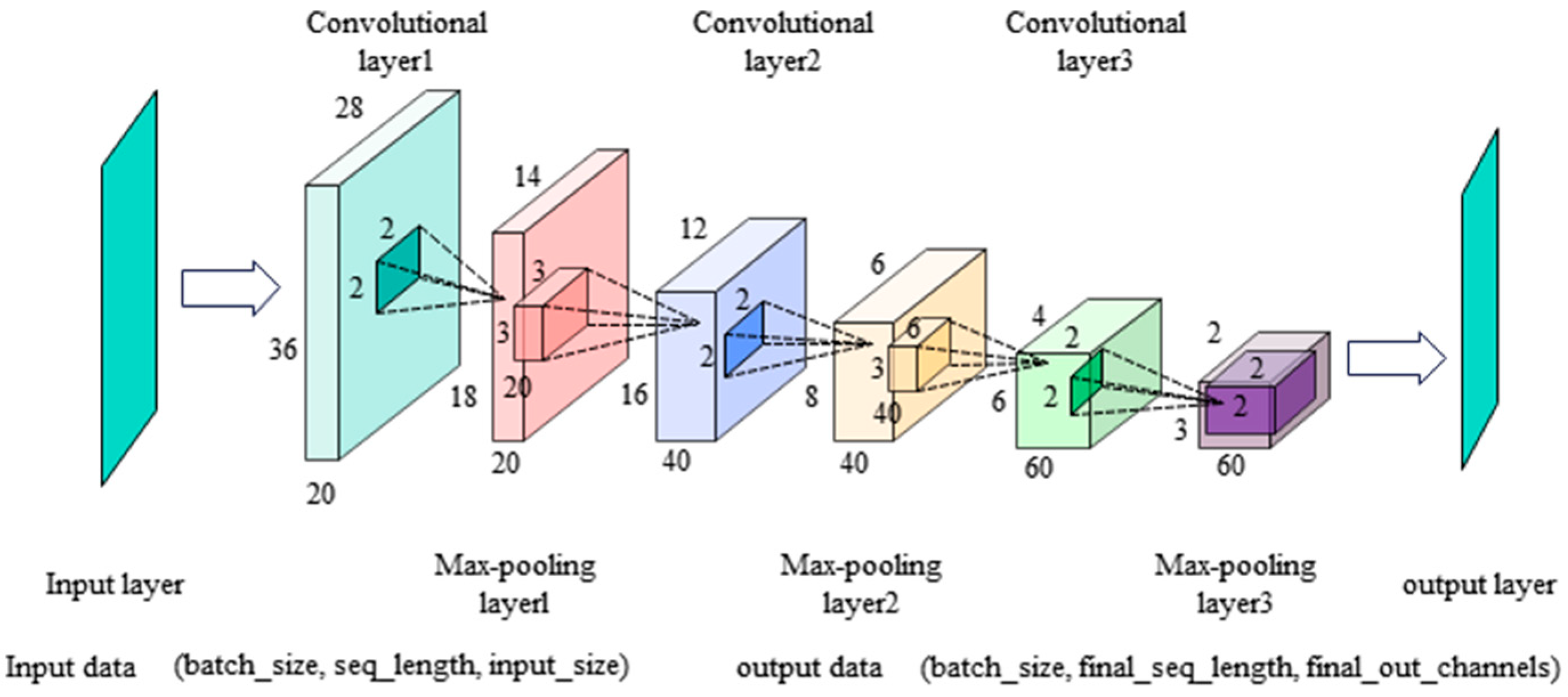
CNNs, a specialized type of deep learning model, have a structure illustrated in Figure 2 when applied to time series feature extraction; this structure includes an input layer that transposes the input data into the shape (batch_size, input_size, seq_length), a convolutional layer that extracts local time series features by converting patterns such as trends and periodicity into higher-level feature representations, a pooling layer that reduces the spatial dimension by selecting the most significant features within the sequence, and an output layer that transforms the resulting data into the format required by subsequent prediction models. For example, employing CNNs to extract spatial features from input data effectively captures the spatial dependence inherent in the data, and the extracted features can then be fed into downstream prediction models to improve their accuracy [18].

2.6. Convolutional Block Attention Module (CBAM)

The CBAM, a lightweight attention mechanism, can be flexibly integrated into various network architectures to enhance their feature representation capabilities, as illustrated in Figure 3; its channel attention module learns the importance weight of each channel through global average pooling followed by a fully connected layer, thereby emphasizing key feature channels, while the spatial attention module employs convolution operations to learn the importance distribution across the spatial dimension of feature maps, enabling the network to focus on critical regions.
For instance, integrating CBAM into the encoder of the Informer model, where features are weighted through channel and spatial attention mechanisms, enables the model to focus more effectively on important features while ignoring irrelevant information, thereby improving the accuracy of AQI prediction [28].
  • Channel attention module
The M C F   output of the channel attention module can be calculated by the following formula:
M C ( F ) = S i g ( M L P A v g p o o l F + M P L M a x p o o l F )
where F denotes the input feature map, AvgPool and MaxPool represent the average pooling and max pooling layers, respectively, MLP refers to the multi-layer perceptron, and Sig denotes the activation function.
2.
The spatial attention module M s ( F ) can be computed using the following formula:
M s F = S i g F n n A v g p o o l F ; M a x p o o l F
where F n n denotes an n × n convolution operation, and A v g p o o l F ; M a x p o o l F represents the concatenation of the average pooling and max pooling results along the channel axis.

2.7. Gated Recurrent Unit (GRU)

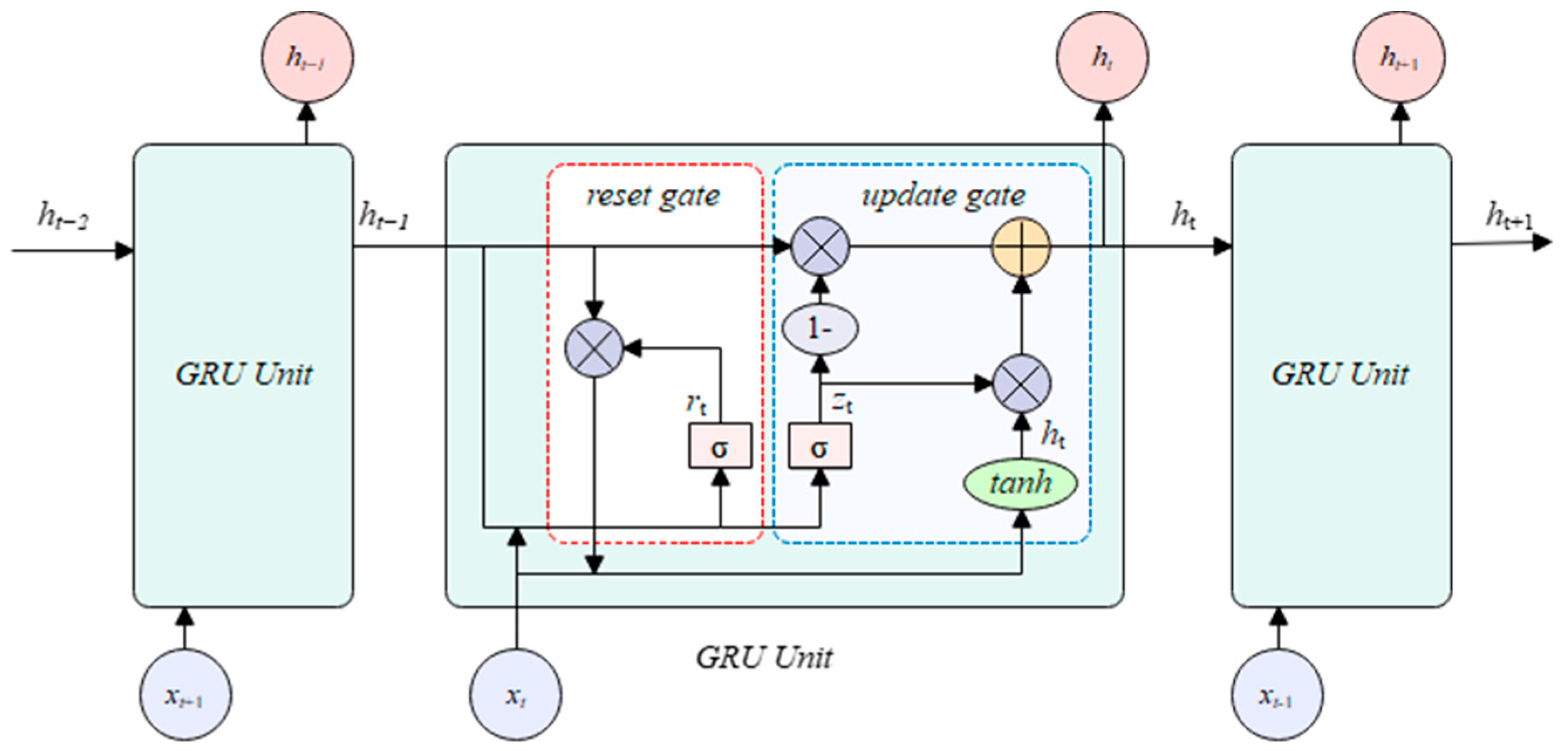
The GRU, an improved version of the traditional recurrent neural network (RNN), introduces update and reset gates to dynamically control the flow of information and the memory update process. Its hidden state not only retains the memory of previous sequences but also has the ability to update or reset information through its gating mechanism. This design enables the network to preserve context over long time periods during sequential tasks while adapting to variations in the data. The core components of GRU—the update gate and reset gate—are illustrated in Figure 4. The update gate determines how much historical information the current state retains, while the reset gate controls how much the current input influences the state. For instance, in AQI prediction, the GRU’s gating mechanism effectively captures both short-term and long-term dependencies in time series data, leading to improved prediction accuracy [15].
The update gate functions to determine how much information from the previous time step should be retained in the hidden state of the current time step. Its output ranges between 0 and 1, where a larger value indicates greater retention of past information, and a smaller value reflects a stronger dependence on the current input. The update gate plays a critical role in balancing the influence of historical and current data during sequence modeling, and its computation is governed by the following formula:
Z t = S i g W z h t 1 , X t + b z
Among them, W z and b z represent the parameter matrix and bias vector, respectively, h t 1 denotes the hidden state from the previous time step, and X t is the current input. Sig refers to the activation function.
The reset gate controls the extent to which the hidden state from the previous time step is ignored. When its output is close to zero, the network tends to “forget” past information and rely primarily on the current input; conversely, when the output approaches one, more information from the previous time step is preserved. This mechanism enables the model to dynamically adjust memory contribution based on the relevance of past data. The calculation formula for the reset gate is as follows:
T t = S i g ( W r h t 1 , X t + b r )
where the sum is the parameter matrix and bias vector of the reset gate W r and b r .

2.8. Study Area and Data Processing

Taking the air quality in Shijiazhuang and Beijing as the research subjects—both being typical representatives of northern cities with significant fluctuations and instability in the AQI—air quality data from June 2021 to June 2023 were selected for the experiment. To evaluate the model’s performance under complex real-world conditions, outliers in the dataset were deliberately left unprocessed. Given the substantial differences in feature scales within the original data, which could potentially prolong training time, a normalization operation was applied to improve the model’s training efficiency by mapping the data to the range (0, 1]. The normalization formula is as follows:
x i = x x m i n x m a x x m i n

3. Results

3.1. Evaluation Metrics

In this study, study areas are Shijiazhuang and Beijing, as shown in Figure 5, 80% of the AQI data was allocated for training and 20% for testing. To assess the predictive performance of the KL-PV-CBGRU model, three evaluation metrics were employed: root mean square error (RMSE), mean absolute error (MAE), and the coefficient of determination (R2), which reflects the model’s degree of fit. The specific calculation formulas for these metrics are as follows:
R M S E = i = 1 n ( y i y l ^ ) 2 n
M A E = i = 1 n y i y ^ l n
R 2 = 1 i = 1 n ( y i y ^ l ) 2 i = 1 n ( y i y ^ ) 2

3.2. Model Time Intervals and Step Selection

The selection of different time intervals and time steps can significantly influence the model’s prediction accuracy. In this study, an interval of 8 (i.e., taking one value every 8 h) and a time step of 3 (i.e., predicting the AQI of the next time point based on the AQI of the previous three time points) were initially considered. To further evaluate the model’s sensitivity to these parameters, four time steps (3, 6, 9, and 12) and four time intervals (1, 8, 16, and 24) were tested in the experiment. The corresponding results are presented in Table 1.
As shown in Table 1, the model demonstrates high accuracy across various combinations of time steps and time intervals. When the time interval is set to 1, the R2 values for all tested time steps exceed 0.99, significantly outperforming the R2 of 0.933 reported for the VMD-TCN model [23]. Even when the time intervals are increased to 8, 16, and 24, the model still maintains a high level of R2 accuracy, indicating its strong predictive capability under different temporal configurations.
The results indicate that the model achieves high accuracy across various combinations of time steps and time intervals, demonstrating its ability to extract multi-scale time series features and capture patterns across different temporal scales. This reflects the model’s strong robustness to variations in data distribution and input volume, as it can adapt effectively to different data characteristics while consistently maintaining high prediction accuracy.

3.3. Comparison Results of Different Models

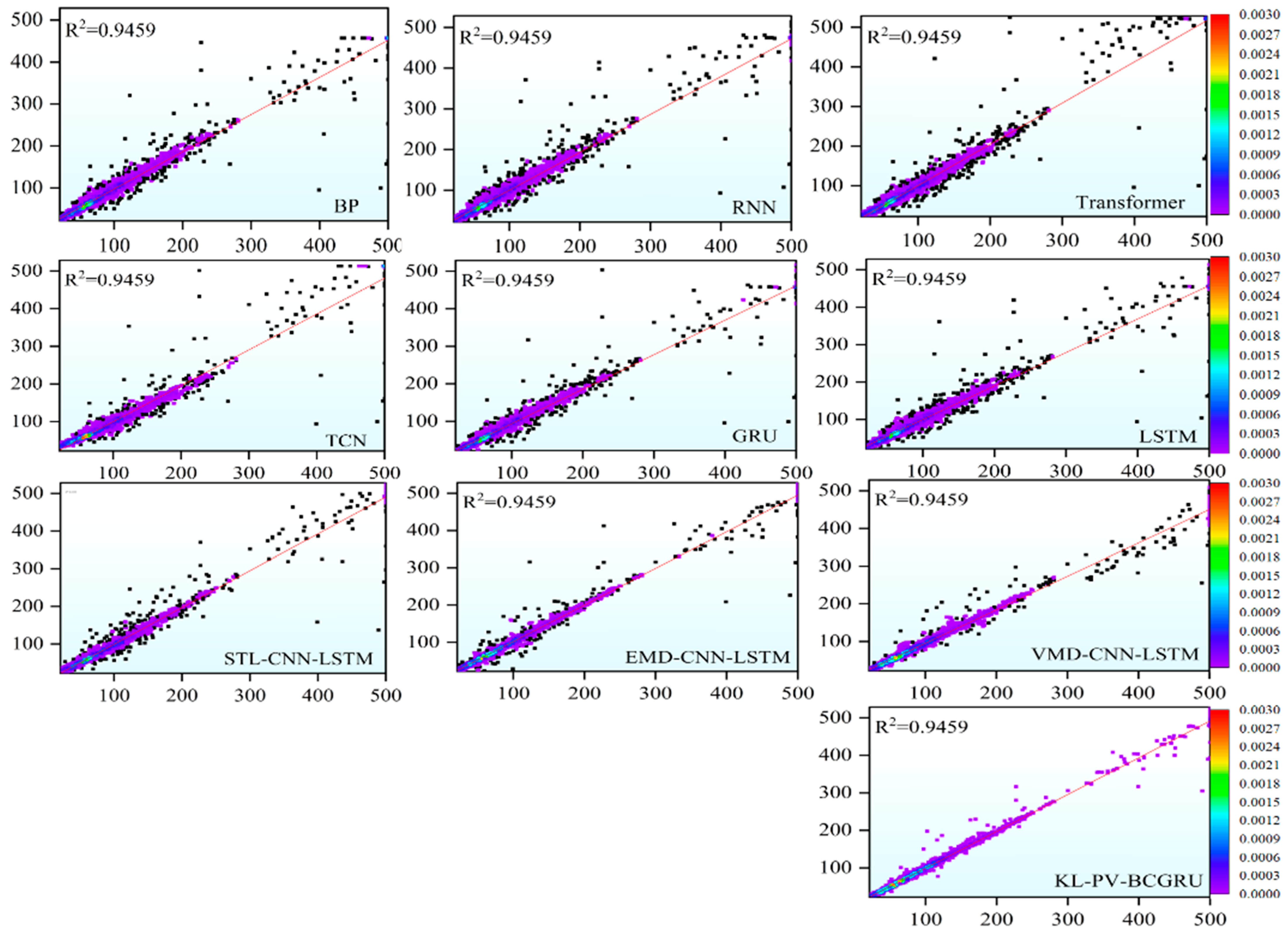
To comprehensively evaluate the performance of the proposed model, nine benchmark models were selected for comparison: LSTM, GRU, RNN, BP, TCN, Transformer, VMD-CNN-LSTM, EMD-CNN-LSTM, and STL-CNN-LSTM. The experimental results are presented in Table 2 and Figure 6.
By comparing the performance of LSTM, GRU, RNN, BP, TCN, and Transformer models, it is observed that when the time interval is 1 h, these single models achieve relatively high accuracy, with average R2 values around 0.95. However, as the time interval increases, their predictive accuracy declines sharply, making it difficult for them to generate effective results. This is primarily due to increased data fluctuations at larger time intervals, which challenge the limited structural capacity of individual models to capture complex temporal patterns. In contrast, the “decomposition–ensemble” hybrid models—VMD-CNN-LSTM, EMD-CNN-LSTM, and STL-CNN-LSTM—demonstrate a notable improvement in predictive accuracy, with R2 values around 0.972 at the 1 h interval. Nonetheless, these models also exhibit reduced accuracy as the time interval increases, with STL-CNN-LSTM experiencing the most pronounced decline.
This decline occurs because, although STL decomposition is well-suited for handling time series with clear seasonality and trends, its effectiveness diminishes as the time interval increases. With larger intervals, AQI data fluctuations become more pronounced, making seasonal and trend components harder to identify. For instance, while STL decomposition may perform well in predicting hourly AQI by capturing recurring patterns such as winter haze peaks, these seasonal signals become blurred at longer intervals, reducing the model’s ability to extract meaningful rules and leading to a drop in prediction accuracy.
In contrast, EMD-CNN-LSTM demonstrates superior performance because EMD is an adaptive signal decomposition method that breaks down AQI data into multiple intrinsic mode functions, each representing fluctuations at different time scales. This approach effectively addresses the nonlinear and non-stationary characteristics of AQI data and enhances the model’s ability to capture local features. For example, in AQI prediction, EMD can separate high-frequency components—such as sudden factory emissions or sandstorms—from low-frequency components like seasonal haze, enabling the model to more accurately capture both short-term and long-term patterns, thereby improving prediction accuracy.
However, VMD-CNN-LSTM achieves the highest accuracy among the compared models, primarily because VMD adaptively decomposes AQI data into multiple subsequences with distinct center frequencies by solving an optimization problem. This approach effectively avoids the mode mixing issue commonly seen in EMD—for instance, where AQI fluctuations caused by factory emissions might be mistakenly attributed to traffic pollution—and is thus better suited for handling complex AQI variations. In AQI prediction, VMD can separate high-frequency modes (such as short-term fluctuations from traffic pollution) from low-frequency modes (such as long-term cumulative effects from industrial emissions), enabling the model to more precisely capture pollution characteristics across different time scales and significantly enhance prediction accuracy.
The KL-PV-CBGRU model proposed in this study achieves an R2 above 0.935, with a value reaching 0.993 at a 1 h time interval. This high accuracy is attributed to the model’s multi-stage decomposition and feature enhancement process. Initially, KL decomposition separates the AQI data into main trend features and residuals, where the residuals—characterized by significant fluctuations—are further decomposed using VMD optimized by PSO. This enables the model to effectively manage complex and dynamic data variations. For example, in AQI prediction, KL decomposes the signal into the primary trend and residuals, the latter potentially representing short-term pollution events or meteorological disturbances. Since residuals often contain high-frequency noise and rapid changes, VMD further decomposes them into distinct frequency modes, allowing the model to better capture pollution characteristics across different time scales. The performance of VMD depends heavily on parameter settings, and PSO is used to adaptively optimize these parameters to enhance decomposition quality. In addition, the feature extraction capability of the CNN module is strengthened through the integration of the CBAM, which helps highlight critical subsequence features. Finally, a bidirectional GRU processes the refined features and reconstructs the prediction results, contributing to the model’s superior overall accuracy.

3.4. Ablation Experiment

In this experiment, the impact of various model components on accuracy was evaluated by selectively eliminating PV from the KL-CBGRU model and CBAM from the KL-PV-CGRU model at one-hour intervals, all under consistent experimental conditions; the corresponding results are presented in Table 3.
As shown in the table, the values of R2, MAE, and RMSE—key indicators of model accuracy—improved significantly due to the impact of double decomposition, with R2 increasing from 0.960 to 0.993, MAE decreasing from 5.187 to 2.397, and RMSE dropping from 14.943 to 6.182, indicating that further reducing residual volatility through quadratic decomposition can enhance the model’s predictive performance. In the case of CNN, the addition of CBAM had a relatively smaller but still positive effect, as R2 rose from 0.987 to 0.993, MAE decreased from 5.254 to 2.397, and RMSE improved from 8.367 to 6.182, suggesting that incorporating CBAM into the CNN architecture strengthens its feature extraction capability and contributes to higher prediction accuracy.

3.5. Model Transfer

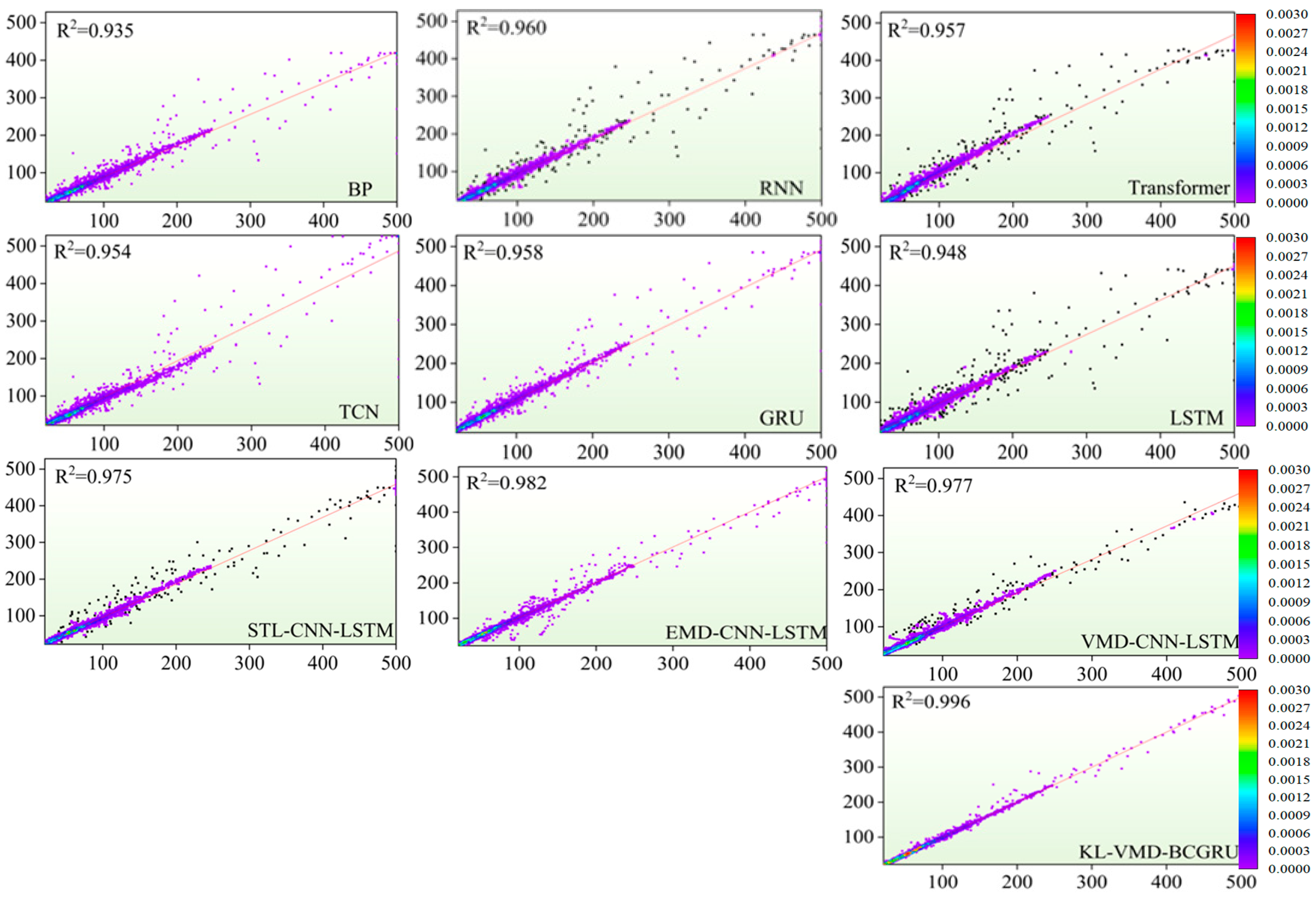
To further evaluate the generalization ability of the model, the Beijing dataset was selected as the experimental data. The same model structure and parameters used for the Shijiazhuang dataset were applied to train the model on the Beijing dataset, allowing for a consistent comparison. This approach enables an assessment of the model’s performance across different datasets within the same framework, providing insights into its generalization capability. The corresponding results and comparisons are presented in Table 4 and Table 5, and Figure 7.
As shown in Table 4, the model demonstrates high accuracy across various time intervals and steps within the Beijing dataset, indicating strong adaptability and flexibility in handling time series data; it maintains stable performance despite variations in data distribution or fluctuations in input volume. Table 5 reveals that, although the model’s accuracy decreases as the time interval increases, it still performs reasonably well, with R2 dropping from 0.996 to 0.909, MAE increasing from 1.723 to 14.547, and RMSE rising from 4.349 to 23.396 as the interval extends from 1 h to 24 h. Figure 6 shows that the scatter density plot of the proposed model is relatively balanced, further confirming the model’s consistent predictive capability. Collectively, these results demonstrate that the proposed model possesses strong generalization and prediction abilities across different regions and temporal conditions.

4. Discussion

Accurate prediction of the AQI under complex conditions is essential for safeguarding public health and safety, as well as for informing effective air pollution control policies. The experimental results demonstrate that the AQI prediction model proposed in this study exhibits strong predictive capability, robustness, and generalization ability, which have been thoroughly validated through experiments conducted on datasets from both Beijing and Shijiazhuang, as detailed below.
  • To address the instability of the AQI, the index is first decomposed into features and residuals using Kalman filtering to reduce overall volatility. However, since the residuals still exhibit significant fluctuations, they are further decomposed using VMD optimized by a PSO algorithm, effectively minimizing their volatility. To overcome the limited predictive capability of a single model, the final prediction is performed using BIGRU integrated with CNN and convolutional attention modules, enhancing both feature extraction and predictive accuracy.
  • The model proposed in this paper demonstrates strong prediction accuracy across various time intervals and time steps, highlighting its robustness and generalization ability in effectively capturing the volatility and instability of AQI under complex conditions. All models introduced in this study achieve high levels of accuracy, with R2, MAE, and RMSE reaching 0.993, 2.397, and 6.182 in Shijiazhuang, and 0.996, 1.723, and 4.349 in Beijing, respectively—surpassing the performance of other deep learning models. The effectiveness of the proposed models has been comprehensively validated through multiple experimental evaluations.
  • This paper has achieved good experimental results by improving the model to predict AQI, but it still avoids the shortcomings of machine learning; that is, it is impossible to make an effective physical and chemical explanation of the prediction process, and the prediction process ignores the influence of meteorological factors. Future work should integrate meteorological data and enhance the interpretability of the model by adding physical and chemical principles to the machine learning model, so as to provide more reliable warnings and stronger support for public health protection and environmental management.

Author Contributions

Funding acquisition, Q.Z.; writing—review and editing, S.C. and Q.Z.; writing—original draft preparation, S.C.; software, S.C.; data curation, Z.C.; methodology, C.Z. and Y.J. All authors have read and agreed to the published version of the manuscript.

Funding

This research was funded by the Central Government Guides Local Science and Technology Development Fund Project (246Z0903G).

Institutional Review Board Statement

Not applicable.

Informed Consent Statement

Not applicable.

Data Availability Statement

Data from China’s environmental testing station “https://quotsoft.net/air/ (accessed on 15 April 2025)”.

Conflicts of Interest

Author Chao Zhang was employed by the company Digital Space Technology Co. The remaining authors declare that the research was conducted in the absence of any commercial or financial relationships that could be construed as a potential conflict of interest.

References

  1. Yao, M.; Wu, G.; Zhao, X.; Li, H.; Chen, J. Estimating health burden and economic loss attributable to short-term exposure to multiple air pollutants in China. Environ. Res. 2020, 183, 109184. [Google Scholar] [CrossRef]
  2. Kim, C.M.; Park, J.S.; Lee, H.; Choi, K.; Smith, D. Association between short-term exposure to air pollution and cardiovascular disease in older adults: A time-stratified case-crossover study in South Korea. Atmos. Environ. 2023, 30, 112–130. [Google Scholar] [CrossRef]
  3. Kai, Y.J.; Dong, X.X.; Miao, F.Y.; Zhang, L.; Huang, R. Impact of ambient air pollution on reduced visual acuity among children and adolescents. Ophthalmic Epidemiol. 2025, 32, 1–8. [Google Scholar] [CrossRef]
  4. Peng, D.; Liu, Y.X.; Sheng, H.Y.; Zhao, Q.; Wang, S. Ambient air pollution and the risk of cancer: Evidence from global cohort studies and epigenetic-related causal inference. J. Hazard. Mater. 2025, 398, 12. [Google Scholar] [CrossRef]
  5. Guo, Z.; Jing, X.; Ling, Y.; Xue, P.; Tan, W. Optimized air quality management based on AQI prediction and pollutant identification in representative cities in China. Sci. Rep. 2024, 14, 17923. [Google Scholar]
  6. Wyat, K.A.; Johnson, O.J.B.; Matthews, M.K.; Lee, S.; Patel, R. The Community Multiscale Air Quality (CMAQ) model versions 5.3 and 5.3.1: System updates and evaluation. Geosci. Model. Dev. 2021, 14, 2867–2897. [Google Scholar]
  7. Yang, W.; Wang, J.; Lu, H.; Zhou, X.; Chen, Y. Hybrid wind energy forecasting and analysis system based on divide-and-conquer scheme: A case study in China. J. Clean. Prod. 2019, 222, 942–959. [Google Scholar] [CrossRef]
  8. Gu, Y.; Zhang, Y.; Zhou, J.; Li, X.; Sun, T. A fuzzy multiple linear regression model based on meteorological factors for air quality index forecast. J. Intell. Fuzzy Syst. 2021, 40, 10523–10547. [Google Scholar] [CrossRef]
  9. Kim, E.S. Ordinal time series model for forecasting air quality index for ozone in Southern California. Environ. Model. Assess. 2017, 22, 175–182. [Google Scholar] [CrossRef]
  10. Liu, H.; Li, Q.; Yu, D.; Chen, L.; Zhao, M. Air quality index and air pollutant concentration prediction based on machine learning algorithms. Appl. Sci. 2019, 9, 4069. [Google Scholar] [CrossRef]
  11. Chatterjee, S.; Roy, A.C. Air quality index assessment prelude to mitigate environmental hazards. Nat. Hazards 2018, 91, 1–17. [Google Scholar] [CrossRef]
  12. Moolchand, S.; Samyak, J.; Sidhant, M.; Verma, P.; Gupta, R. Forecasting and prediction of air pollutant concentrations using machine learning techniques: The case of India. IOP Conf. Ser. Mater. Sci. Eng. 2021, 1022, 012123. [Google Scholar]
  13. Su, Y.; Xie, H. Prediction of AQI by BP neural network based on genetic algorithm. In Proceedings of the 5th International Conference on Automation, Control and Robotics Engineering (CACRE 2020), Dalian, China, 19–20 September 2020; School of Science, Dalian Maritime University: Dalian, China, 2020; pp. 650–654. [Google Scholar]
  14. Maleki, H.; Sorooshian, A.; Goudarzi, G.; Farzanegan, A.; Li, X. Air pollution prediction by using an artificial neural network model. Clean. Technol. Environ. Policy 2019, 21, 1341–1352. [Google Scholar] [CrossRef] [PubMed]
  15. Kumar, A.M.; Rikta, S. Medium-term AQI prediction in selected areas of Bangladesh based on bidirectional GRU network model. SN Comput. Sci. 2024, 5, 112–125. [Google Scholar] [CrossRef]
  16. Kumar, S.N.; Prakash, S.; Daniel, A.; Venkatesh, P.; Rao, K. Optimized machine learning model for air quality index prediction in major cities in India. Sci. Rep. 2024, 14, 6795. [Google Scholar] [CrossRef] [PubMed]
  17. Jia, Z.; Baofeng, L.; Hong, C.; Zhang, Y. AQI multi-point spatiotemporal prediction based on K-means clustering and RNN-LSTM model. J. Phys. Conf. Ser. 2021, 2006, 012034. [Google Scholar]
  18. Zhu, X.; Zou, F.; Li, S.; Wang, T.; Sun, Z. Enhancing air quality prediction with an adaptive PSO-optimized CNN-Bi-LSTM model. Appl. Sci. 2024, 14, 5787. [Google Scholar] [CrossRef]
  19. Sarkar, N.; Keserwani, K.P.; Govil, C.M.; Verma, S. A modified PSO-based hybrid deep learning approach to predict AQI of urban metropolis. Urban Clim. 2024, 19, 102212. [Google Scholar] [CrossRef]
  20. Wang, J.; Li, X.; Wang, T.; Chen, Y.; Liu, H. A CA-GRU-based model for air quality prediction. Int. J. Ad. Hoc Ubiquitous Comput. 2021, 38, 184–198. [Google Scholar] [CrossRef]
  21. Qian, S.; Peng, T.; He, R.; Zhang, L.; Liu, Y. A novel ensemble framework based on intelligent weight optimization and multi-model fusion for air quality index prediction. Urban Clim. 2024, 25, 33–47. [Google Scholar] [CrossRef]
  22. Zhu, S.; Lian, X.; Liu, H.; Wang, P.; Zhao, Q. Daily air quality index forecasting with hybrid models: A case in China. Environ. Pollut. 2017, 231, 1232–1244. [Google Scholar] [CrossRef] [PubMed]
  23. Shi, X.; Tang, Z.; Zhang, Z.; Li, F.; Chen, G. A new decomposition-integrated air quality index prediction model. Earth Sci. Inform. 2023, 16, 2307–2321. [Google Scholar]
  24. Zhang, S.; Wang, P.; Wu, R.; Li, M.; Zhao, Y. CEEMD-LASSO-ELM nonlinear combined model of air quality index prediction for four cities in China. Environ. Ecol. Stat. 2023, 30, 309–334. [Google Scholar]
  25. Dalal, S.; Lilhore, K.U.; Faujdar, N.; Singh, P. Optimising air quality prediction in smart cities with hybrid particle swarm optimization–LSTM–RNN model. IET Smart Cities 2024, 6, 156–179. [Google Scholar] [CrossRef]
  26. Chen, J.; Chen, K.; Ding, C.; Wang, G.; Liu, Q.; Liu, X. An Adaptive Kalman Filtering Approach to Sensing and Predicting Air Quality Index Values. IEEE Access 2020, 8, 4265–4272. [Google Scholar] [CrossRef]
  27. Dragomiretskiy, K.; Zosso, D. Variational mode decomposition. IEEE Trans. Signal Process. 2014, 62, 531–544. [Google Scholar] [CrossRef]
  28. Dong, X.; Li, D.; Wang, W.; Zhang, Q.; Liu, J. BWO-CAformer: An improved Informer model for AQI prediction in Beijing and Wuhan. Process Saf. Environ. Prot. 2025, 195, 106800. [Google Scholar] [CrossRef]
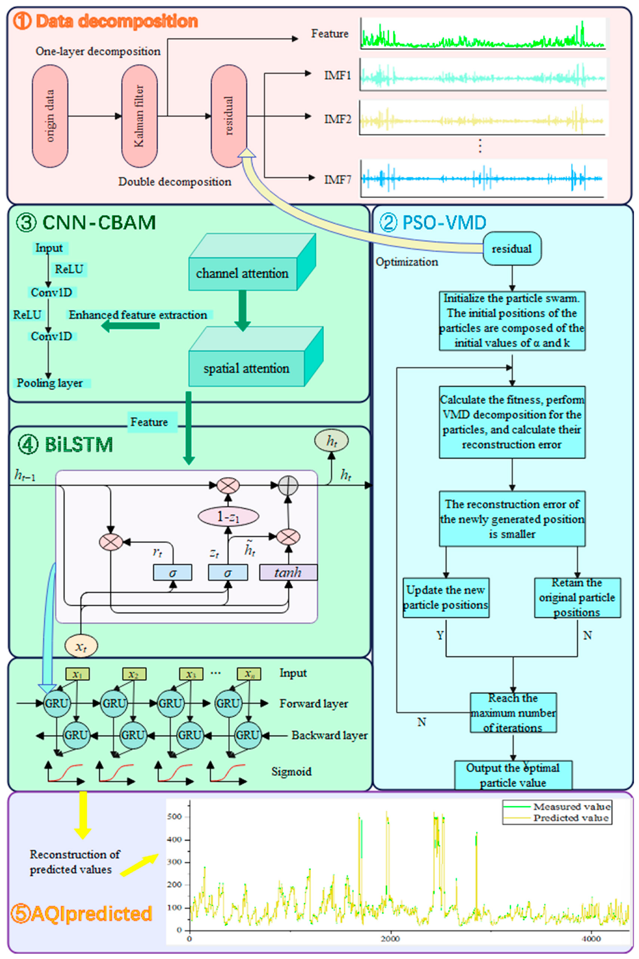
Figure 1. Technology roadmap.
Atmosphere 16 00965 g001
Figure 2. Schematic diagram of CNN.
Atmosphere 16 00965 g002
Figure 3. Schematic diagram of the CBAM structure.
Atmosphere 16 00965 g003
Figure 4. Schematic diagram of GRU.
Atmosphere 16 00965 g004
Figure 5. Beijing and Shijiazhuang.
Atmosphere 16 00965 g005
Figure 6. Scatter density plots of different prediction models in Shijiazhuang.
Atmosphere 16 00965 g006
Figure 7. Scatter density plots of different models in Beijing.
Atmosphere 16 00965 g007
Table 1. Accuracy of Shijiazhuang data at different time intervals and steps.
Time StepR2(1)MAERMSER2(8)MAERMSER2(16)MAERMSER2(24)MAERMSE
30.9922.8936.4810.9589.30015.3570.91113.63321.9930.92215.92825.071
60.9932.3976.1820.9628.96214.6370.93211.08119.2680.94014.03522.108
90.9902.9936.6810.9628.53514.7350.93311.15819.0140.93314.04723.357
120.9932.4806.0570.9638.66814.3910.93511.00118.8210.93514.26722.907
Table 2. Accuracy comparison of different models in Shijiazhuang.
ModelR2(1)MAERMSER2(8)MAERMSE
LSTM0.94697.376617.20260.536925.807251.1200
GRU0.94857.741316.94670.564225.365249.5876
RNN0.94636.925517.31100.546825.721850.5703
BP0.94816.814417.01170.518426.337652.1308
TCN0.94597.934017.37040.515926.438652.2667
Transformer0.94046.776318.23900.510727.136652.5444
VMD-CNN-LSTM0.97215.908112.47940.86116.51028.0094
EMD-CNN-LSTM0.97784.961311.13580.76220.13136.739
STL-CNN-LSTM0.97185.434412.54680.811619.160632.6334
KL-PV-CBGRU0.9932.3976.1820.9638.66814.391
ModelsR2(16)MAERMSER2(24)MAERMSE
LSTM0.274132.521162.77650.273138.488576.6695
GRU0.281235.369862.46890.254640.780877.6354
RNN0.298232.658761.72930.262140.672177.2483
BP0.323532.566660.60660.233538.062578.7288
TCN0.291432.008262.02730.246438.254078.0645
Transformer0.301635.811661.57780.241738.984778.3053
CNN-LSTM-VMD0.841818.070429.30390.811622.670339.0332
CNN-LSTM-EMD0.679025.729041.75000.619435.325455.4775
STL-CNN-LSTM0.640326.570044.19200.376839.702070.9900
KL-PV-CBGRU0.93511.00118.8210.94014.03522.108
Table 3. Comparison of ablation experiments.
ModelsR2 MAERMSE
KL-PV-CGRU0.9875.2548.367
KL-PV-CBGRU0.9932.3976.182
KL-CBGRU0.9605.81714.943
Table 4. Precision of Beijing data at different time intervals and steps.
Time StepsR2(1)MAERMSER2(8)MAERMSER2(16)MAERMSER2(24)MAERMSE
30.9961.7814.3450.9509.55516.1680.92013.42220.9850.8790.87927.000
60.9952.1184.8450.9509.63216.1980.94011.77018.1660.90215.16824.317
90.9961.7234.3490.9519.27916.0420.94111.58317.9860.90914.54723.396
120.9961.9614.5090.9509.44216.1770.95010.98516.5280.90514.52823.885
Table 5. Precision comparison of different models in Beijing.
Model R2(1)MAERMSER2(8)MAERMSE
LSTM0.94816.866115.76420.474226.323552.3974
GRU0.95849.344314.10720.467826.416852.7193
RNN0.96017.420313.82450.461526.618053.0262
BP0.93569.074417.55830.468827.184352.6663
TCN0.95416.783014.82930.430426.885454.5387
Transformer0.95756.388014.25980.455527.906553.3249
CNN-LSTM-VMD0.97785.928610.32160.871715.305225.9079
VMD-CNN-LSTM0.98274.58899.10190.739221.241836.9375
STL-CNN-LSTM0.97535.164710.87670.595324.517646.0082
KL-PV-CBGRU0.9961.7234.3490.9519.27916.042
ModelR2(16)MAERMSER2(24)MAERMSE
LSTM0.244436.113464.31830.005239.889877.3441
GRU0.239834.596264.51470.008940.312377.1996
RNN0.204535.822165.99380.007140.289177.2693
BP0.219533.429265.37150.066340.756974.9304
TCN0.245533.631764.26950.107339.474273.2669
Transformer0.239634.416964.52360.108139.926573.2339
CNN-LSTM-VMD0.833918.117630.15780.773522.837736.9064
CNN-LSTM-EMD0.524831.769051.00440.330437.619663.4538
STL-CNN-LSTM0.560329.083849.06540.172940.065970.5240
KL-PV-CBGRU0.95010.98516.5280.90914.54723.396
Disclaimer/Publisher’s Note: The statements, opinions and data contained in all publications are solely those of the individual author(s) and contributor(s) and not of MDPI and/or the editor(s). MDPI and/or the editor(s) disclaim responsibility for any injury to people or property resulting from any ideas, methods, instructions or products referred to in the content.