Article

A Spatiotemporal Multimodal Framework for Air Pollution Prediction Based on Bayesian Optimization—Evidence from Sichuan, China

College of Management Science, Chengdu University of Technology, Chengdu 610059, China
*
Author to whom correspondence should be addressed.
Atmosphere 2025, 16(8), 958; https://doi.org/10.3390/atmos16080958
Submission received: 9 June 2025 / Revised: 30 July 2025 / Accepted: 8 August 2025 / Published: 11 August 2025
(This article belongs to the Special Issue Applications of Artificial Intelligence in Atmospheric Sciences)

Abstract

In regions characterized by complex terrain and diverse pollution sources, high-precision air pollution prediction remains challenging due to nonlinear spatiotemporal coupling and the difficulty of modeling local pollutant agglomeration. To address these issues, this study proposes a CNN–LSTM–Transformer multimodal prediction framework integrated with Bayesian Optimization. First, the Local Moran’s Index (LMI) is introduced as a spatial perception feature and concatenated with pollutant concentration sequences before being input into the CNN module. This design enhances the model’s ability to identify local pollutant clustering and spatial heterogeneity. Second, the LSTM architecture adopts a dual-channel structure: the main channel employs bidirectional LSTM to extract temporal dependencies, while the auxiliary channel uses unidirectional LSTM to capture evolutionary trends. A Transformer with a multi-head attention mechanism is then introduced to perform global modeling. Bayesian Optimization is employed to automatically adjust key hyperparameters, thereby improving the model’s stability and convergence efficiency. Empirical results based on atmospheric pollution monitoring data from Sichuan Province during 2021–2024 demonstrate that the proposed model outperforms various mainstream methods in predicting six pollutants in Chengdu. For instance, the MAE for PM2.5 decreased by 14.9–22.1%, while the coefficient of determination (R2) remained stable between 87% and 89%. The accuracy decay rate across four-day forecasts was controlled within 12.4%. Furthermore, in PM2.5 generalization prediction tasks across four other cities—Yibin, Zigong, Nanchong, and Mianyang—the model exhibited superior stability and robustness, achieving an average R2 of 87.4%. These findings highlight the model’s long-term stability and regional generalization capability, offering reliable technical support for air pollution prediction and control strategies in Sichuan Province and potentially beyond.

1. Introduction

The World Health Organization reports that approximately 7 million people die prematurely each year from air pollution globally, with China accounting for roughly 30% of these deaths [1]. This alarming reality stems directly from China’s coal-dominated energy structure and rapid urbanization processes. The research demonstrates that coal combustion contributes 38–45% of PM2.5 pollution sources in China [2]. Vehicle emissions account for 50–60% of the nitrogen oxide (NOₓ) pollution sources [3]. Industrial processes serve as the primary source of volatile organic compounds (VOCs), contributing over 40% of total emissions [4]. These major pollution sources collectively generate various atmospheric pollutants, most commonly PM2.5, PM10, SO2, NO2, O3, and CO [5]. Notably, pollutant concentrations respond not only to emission source intensity but also to significant meteorological controls. The research shows that stable winter weather conditions—characterized by relative humidity exceeding 60% and mixing layer heights below 500 m—substantially weaken pollutants’ vertical diffusion and horizontal transport capacity, reducing dispersion efficiency by 50–70% [6]. These unfavorable meteorological conditions directly cause persistent pollutant accumulation at ground level, becoming a critical factor in frequent winter pollution outbreaks across regions like Beijing, Tianjin and Hebei. Consequently, daily average PM2.5 concentrations often exceed 150 μg/m3 [7], far surpassing the WHO’s daily safety limit of 15 μg/m3. Long-term exposure to such highly polluted environments substantially increases health risks, including respiratory diseases, chronic obstructive pulmonary disease (COPD), and lung cancer, potentially leading to premature death [8]. Therefore, using high-precision prediction models to capture the fluctuation characteristics of air pollutants can provide scientific support for pollution prevention and early warning and effectively reduce the losses caused by pollution.
In the field of air quality prediction, mainstream approaches can be broadly categorized into two types: deterministic models and statistical modeling methods. Deterministic models are based on atmospheric physicochemical mechanisms and simulate pollutant emission, dispersion, transport, and chemical transformation processes by solving partial differential equations. Representative models in this category include the Community Multi-scale Air Quality Model (CMAQ), the Weather Research and Forecasting model coupled with Chemistry (WRF–Chem), and the Comprehensive Air Quality Model with Extensions (CAMx) [9]. Deterministic models possess strong physical interpretability and are particularly suitable for policy intervention simulations and scenario assessments. However, these models exhibit high dependence on initial boundary conditions, pollutant emission inventories, and meteorological input data. Moreover, they involve substantial computational costs and often struggle to meet real-time prediction requirements at high spatiotemporal resolutions [10].
Therefore, researchers have gradually shifted toward an alternative modeling approach based on historical observational data—statistical modeling methods. This category of methods has become another important research direction in atmospheric pollution prediction, distinct from deterministic models, due to their simple structure, high computational efficiency, and good adaptability in small- to medium-scale data-driven tasks. Early studies in this area primarily employed classical models such as Multiple Linear Regression (MLR) [11] and Autoregressive Integrated Moving Average (ARIMA) [12] to model trends in pollutant concentration changes. These traditional statistical models demonstrate certain advantages in handling linear relationships. However, they generally rely on data stationarity and completeness, and their predictive performance and generalization ability decline significantly when observational data contain missing values, noise, or abrupt changes [13]. Additionally, as pollution causes become increasingly complex and high-dimensional, multi-source data are continuously introduced, and the limitations of these models in feature extraction capability and adaptation to complex environmental changes have become increasingly apparent. This is particularly evident in their inadequate performance in characterizing nonlinear coupling relationships between pollutants and environmental factors such as meteorology and topography.
Against this background, researchers have gradually turned to machine learning methods with stronger feature representation and generalization capabilities. For example, a support vector machine (SVM) [14], Multilayer Perceptrons (MLPs) [15], and Random Forest (RF) [16] improve the ability of the model to capture feature changes to some extent. Compared with traditional methods, these models have a stronger fitting ability and do not need to define the function form. However, with the deepening of the research on the spatiotemporal evolution mechanism of the pollution process, the limitations of these models in modeling long-term dependence and deep feature interaction begin to appear gradually. Based on this, researchers began to turn to deep learning methods with more representational ability in order to seek better prediction results.
Typical models include a recurrent neural network (RNN) [17], the long-term and short-term memory network (LSTM) [18], the convolutional neural network (CNN) [19] and so on. These models can effectively capture the inherent time-dependent relationship and complex nonlinear relationship in air pollution dynamics. Taking CNN as an example, Huang et al. (2019) [20] put forward an RNN–CNN integrated framework, and achieved a goodness of fit of more than 0.97 on 34% sites, which verified its advantages in PM2.5 Hourly concentration prediction. However, CNN can only effectively extract short-term or local features, and there are still shortcomings in capturing long-term dependence and global features; LSTM is excellent in capturing the long-term and short-term dependence, especially suitable for forecasting the time series of air pollutants. The research of Shi et al. (2022) [21] shows that LSTM can well predict the daily variation trend of PM2.5. However, due to the problem of long-range dependent attenuation, the LSTM model is still insufficient in long-time span and complex nonlinear feature extraction, and it is difficult to model complex global dynamic features completely [22].
Due to the inherent nonlinearity and irregularity of air pollutants, many deep learning models still have shortcomings in feature interaction and integration of complex environmental variables, which leads to limited prediction accuracy and generalization ability of the models [23]. In view of the limitations of a single model, scholars have explored multi-model fusion methods in recent years to improve the prediction performance and the generalization ability of the model. One method focuses on structural integration, such as the CNN–LSTM combined model proposed by Zhang et al. (2022) [24], which complements and fuses spatial and temporal feature extraction, effectively making up for the deficiency of single model in representation ability; the VMD–Transformer–ECM combined framework proposed by Zhang et al. (2024) [25] improves the multi-scale feature analysis ability through modal decomposition, error compensation and context modeling of the Transformer. A neural network model based on frequency domain information and bidirectional long-term and short-term memory (FD–BiLSTM), as constructed by Tang et al. [26], enhances the bidirectional modeling ability by using BiLSTM to learn the dependency relationship before and after. Another method focuses on parameter optimization and structural adjustment, such as the Bayesian optimization gated cyclic unit neural network (BO–GRU) model proposed by Jia et al. [27], which adopts a Bayesian optimization algorithm to improve the efficiency of super-parameter search; Niu et al. [28] optimized the structure of CNN–BiGRU–Attention through the sparrow search algorithm, which enhances the feature learning ability; the ARIMA–WOA–LSTM hybrid model developed by Luo et al. [29] improves the LSTM network using the whale optimization algorithm (WOA) to realize an accurate prediction of the nonlinear residual sequence. In addition, to systematically summarize the technical evolution characteristics of existing representative models in structural fusion and parameter optimization, Table 1 provides a comparative analysis of different methods regarding their spatiotemporal feature modeling capabilities, regional generalization ability, and hyperparameter optimization mechanisms.
As can be seen from Table 1 above, although the existing fusion models have made some progress in improving the performance of air pollution prediction, there are still many limitations. On the one hand, most models still focus on the shallow structure of single-channel LSTM in time–space dependence modeling, which can not fully capture the long-term evolution law and nonlinear interaction characteristics of pollutant concentration. On the other hand, although some studies introduce the attention mechanism structure such as Transformer, they lack in-depth analysis of spatial aggregation mode and the synergistic relationship between meteorological factors and pollutants, which makes it difficult for the model to adapt to the actual environment with strong regional heterogeneity and complex variable coupling. In addition, a large number of existing explorations ([24,25,26]) generally rely on manual experience or grid search, which can easily fall into local optimization and restrict the generalization ability and stability of the model.
In order to solve the above problems, this paper proposes an air pollutant prediction framework that integrates Bayesian optimization and multimodal deep neural network, and integrates convolutional neural network (CNN), dual-channel long-term short-term memory network (Bi–LSTM and deep one-way LSTM) and Transformer encoder to realize the collaborative modeling of spatial structure, time dependence and multi-source characteristics of pollutant concentration. Compared with existing methods such as CNN–LSTM–Transformer or BO–CNN–LSTM, this study has the following four innovations:
(1)
The Local Moran’s Index (LMI) is introduced to quantify the spatial autocorrelation of pollutant concentrations between each monitoring station and its neighboring sites. Combined with pollutant concentration sequences, LMI features are incorporated into the CNN module to provide localized spatial structural information and to support the characterization of current pollution dispersion patterns.
(2)
Build a two-channel LSTM architecture in which Bi–LSTM is used in the main channel to model the two-way dependence of time series, and three-layer unidirectional LSTM is used in the auxiliary channel to enhance the ability to extract the one-way evolution trend of pollutant concentration, so as to realize the deep decoupling modeling of multi-scale time dynamics.
(3)
Combined with the multi-head self-attention mechanism of the Transformer encoder, the global dynamic modeling among pollutants, meteorological factors and spatial characteristics is realized.
(4)
The Bayesian optimization algorithm is introduced to adaptively adjust the key super-parameters such as learning rate, LSTM layer number and Dropout rate, so as to comprehensively improve the prediction accuracy, stability and generalization ability of the model.

2. Materials and Methods

2.1. Study Area

This study takes Sichuan Province in the southwest hinterland of China as the research area (geographical coordinates 97°21′–108°31′ E, 26°03′–34°19′ N), with a total area of 486,000 square kilometers and a permanent population of over 83.64 million, which is one of the key areas for air pollution prevention and control in China. At the same time, Sichuan Province is also the only provincial administrative region in China that is located in the basin. Its unique landform pattern is jointly constructed by Qinling–Daba Mountain, Hengduan Mountain and Wushan Mountain, forming a closed topographic structure. In terms of climate characteristics, dominated by the law of vertical zonality differentiation, the climate system in the province presents a continuous pedigree from subtropical semi-humid climate to alpine cold temperate climate. The coupling effect of this special terrain condition and high-frequency static weather significantly weakens the horizontal diffusion ability of atmospheric pollutants, leading to the prominent phenomenon of regional pollution agglomeration. At the same time, it is limited by the obvious difference of altitude gradient within the province: the average altitude in Hengduan Mountain area in the west exceeds 4000 m, and it drops sharply to Sichuan Basin with an average altitude of about 400 m in the east. This steep terrain drop makes pollutants easy to settle in the low-altitude Chengdu Plain economic circle, which poses a severe challenge to regional sustainable development. See Figure 1 for the spatial distribution of the study area.

2.2. Data Collection and Preprocessing

2.2.1. Main Features

In this study, six kinds of air pollutants routinely monitored by ambient air quality monitoring stations were selected as the research objects, including fine particles (PM2.5), inhalable particles (PM10), sulfur dioxide (SO2), nitrogen dioxide (NO2), carbon monoxide (CO) and ozone (O3). Specifically, ozone is represented by its maximum daily 8 h average concentration (MDA8), which is consistently used throughout the analysis. The daily concentration data of pollutants are all from 123 state-owned monitoring stations in Sichuan Province, recorded by the National Urban Air Quality Real-time Release Platform of China Environmental Monitoring Center (https://www.cnemc.cn/). See Figure 1c for the site distribution, and the monitoring data duration is from 1 January 2021 to 30 June 2024.

2.2.2. Data Processing

In order to ensure the accuracy and stability of the model prediction, the original monitoring data set is first detected and interpolated. Specifically, firstly, the time series is standardized, and the time stamp calibration and continuity check are carried out on the observation data of six kinds of pollutants at all stations. According to 95% missing data threshold, 104 effective monitoring stations were screened out. In order to ensure the integrity of the time series, a complete daily series covering 1 January 2021 to 30 June 2024 was reconstructed. Then, two statistical methods are used to identify and eliminate outliers. On the one hand, based on the 3σ rule, the global extreme value that deviates from the mean value by more than 3 times the standard deviation is eliminated; On the other hand, the interquartile distance (IQR) method is used to identify local outliers, and the points beyond the range of 1.5 times IQR above and below are marked as missing values. For the vacancy caused by missing values and abnormal elimination, this paper adopts the following three-stage interpolation method to fill it: (1) linear interpolation to fill the small range of missing between adjacent time points; (2) second-order spline interpolation smoothes the temporal variation trend of pollutant concentration; (3) fill the residual missing value at the boundary of the completion sequence forward/backward.
Comparing the original and processed data sets (see Table 2), the number of valid sites has decreased from 123 to 104, the missing rate has decreased from 17.70% to 0%, the proportion of abnormal values has decreased significantly, and the integrity and quality of data coverage have improved significantly. After the interpolation is completed, this paper re-verifies the data quality from the perspectives of maximum and minimum changes, the proportion of abnormal values and the distribution of unique values. The results show that the interpolation does not introduce abnormal mutation, a few stations show low variability because of the stable pollution concentration itself, and the overall interpolation effect is reasonable, which does not cause excessive smoothing or information distortion. The detailed technical workflow of this study is shown in Figure 2.

2.2.3. Local Moran’s Index Feature Modeling

To enhance the model’s ability to perceive spatial heterogeneity, this study introduces the Local Moran’s Index (LMI) to construct spatial perception features [30]. LMI quantifies the degree of spatial autocorrelation in pollutant concentrations between each monitoring station and its neighboring stations, providing the model with local spatial structure information. Considering that the original LMI values have a relatively small range (typically between −1 and 1), this study adopts an adaptive standardization strategy. The LMI features are standardized to a numerical scale comparable to pollutant concentrations to ensure effective propagation in deep networks. Specifically, LMI features are concatenated with original pollutant concentration sequences as joint inputs to the model. During the one-dimensional convolution (Conv1D) stage, they help identify local spatial patterns, while in the LSTM and Transformer stages, they provide spatial structure information support for temporal dynamics and global dependency modeling. This approach enables the model to capture local pollution agglomeration phenomena and spatial heterogeneity changes more sensitively while maintaining its original temporal feature extraction capability. Consequently, it significantly improves generalization performance in complex geographical environments. Notably, LMI not only provides the degree of spatial clustering for current station pollution conditions but also offers the model a “dynamic spatial weight adjustment signal.” When pollutants exhibit regional clustering, LMI shows positive values, guiding the model to enhance perception and response to neighborhood features. Conversely, when station concentrations deviate from neighborhood average levels, LMI becomes negative, suggesting that the model should rely more on its own temporal features for prediction. The introduction of this “structure-aware input feature” enables the model to dynamically balance local observations with neighborhood relationships when facing complex terrain and heterogeneous spatial distributions, thereby improving overall prediction accuracy and stability.

2.3. Methodology

2.3.1. Framework Overview

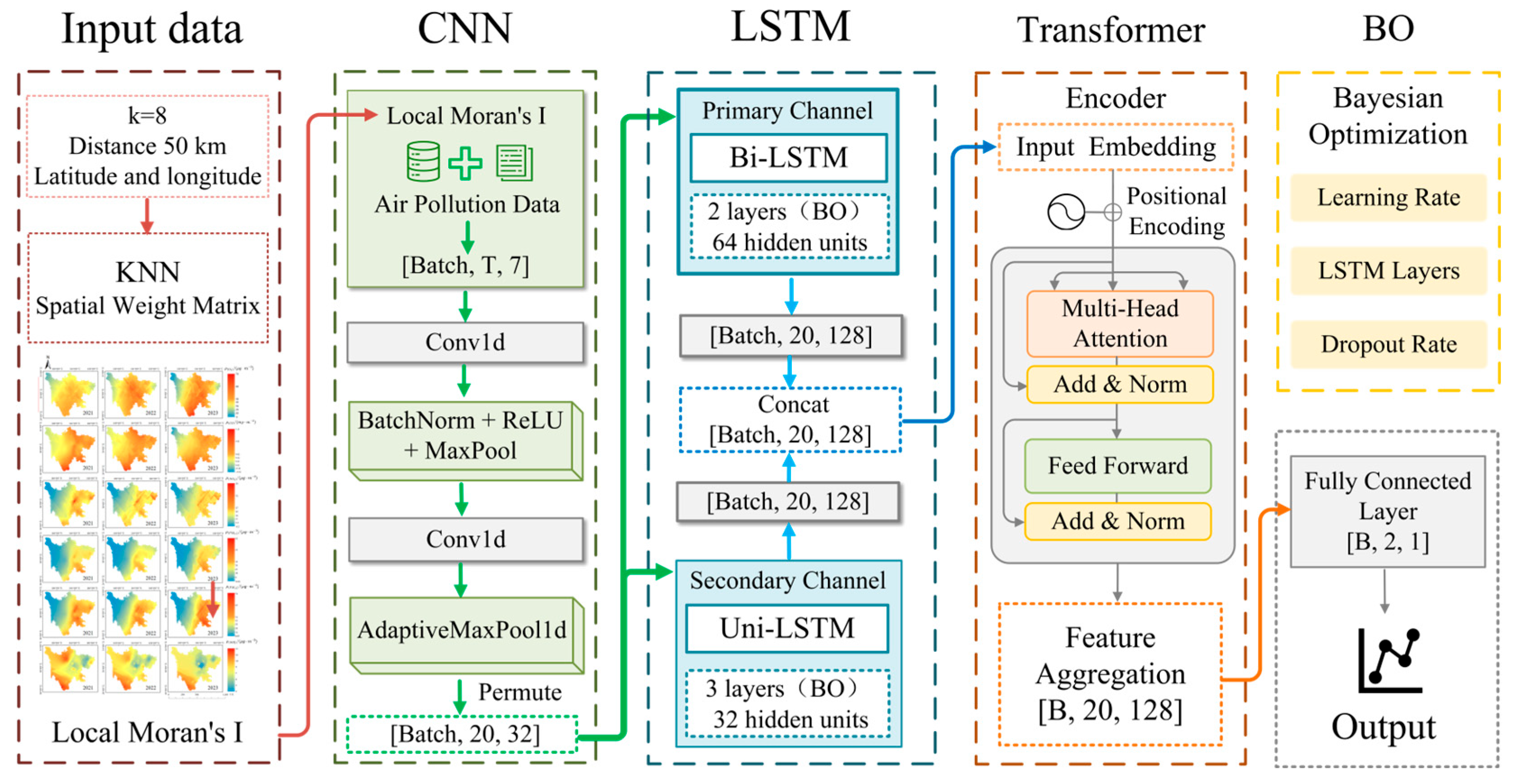
To address challenges such as spatial heterogeneity, seasonal variability, and complex variable interactions in air pollution prediction, this study proposes an integrated deep learning prediction framework (Figure 3) that combines Convolutional Neural Networks (CNN), Long Short-Term Memory networks (LSTM), Transformer encoders, and Bayesian Optimization (BO). The framework consists of four key stages: spatial feature computation, temporal modeling, global feature modeling, and hyperparameter optimization. First, based on the geographic coordinates and average pollutant concentrations at each monitoring site, the model employs the K-Nearest Neighbors (KNN) algorithm to construct a spatial weight matrix and calculate the Local Moran’s I index, thereby quantifying the spatial clustering effect of pollutants. These spatial indices are then fused with atmospheric observation data using a 1D CNN to extract multi-dimensional spatial features, forming spatially informed feature datasets. This dataset is subsequently fed into a dual-channel LSTM structure for temporal modeling. In the dual-channel design, the primary channel utilizes a bidirectional LSTM to capture both forward and backward temporal dependencies, while the auxiliary channel employs a three-layer unidirectional LSTM to enhance the modeling of unidirectional trends in pollutant concentration evolution. The outputs from both channels are concatenated along the feature dimension to form a 128-dimensional hybrid temporal feature vector, which serves as input to the Transformer encoder. Within the LSTM architecture, key hyperparameters—including learning rate, number of LSTM layers, and dropout rate—are automatically tuned using Bayesian Optimization. This strategy improves the model’s predictive performance and enhances its generalization ability. Subsequently, two layers of Transformer encoders are applied to the hybrid sequence for global feature modeling. By integrating positional encoding and multi-head self-attention mechanisms, the Transformer captures cross-timestep feature dependencies. Additionally, a gating mechanism is introduced to dynamically weight the Transformer outputs, thereby improving the model’s sensitivity to sudden pattern shifts. Finally, the globally contextualized features—obtained via temporal average pooling—and the end-of-sequence state are fused and passed through a fully connected layer to complete the one-step prediction of pollutant concentrations.

2.3.2. Dual-Channel LSTM Architecture

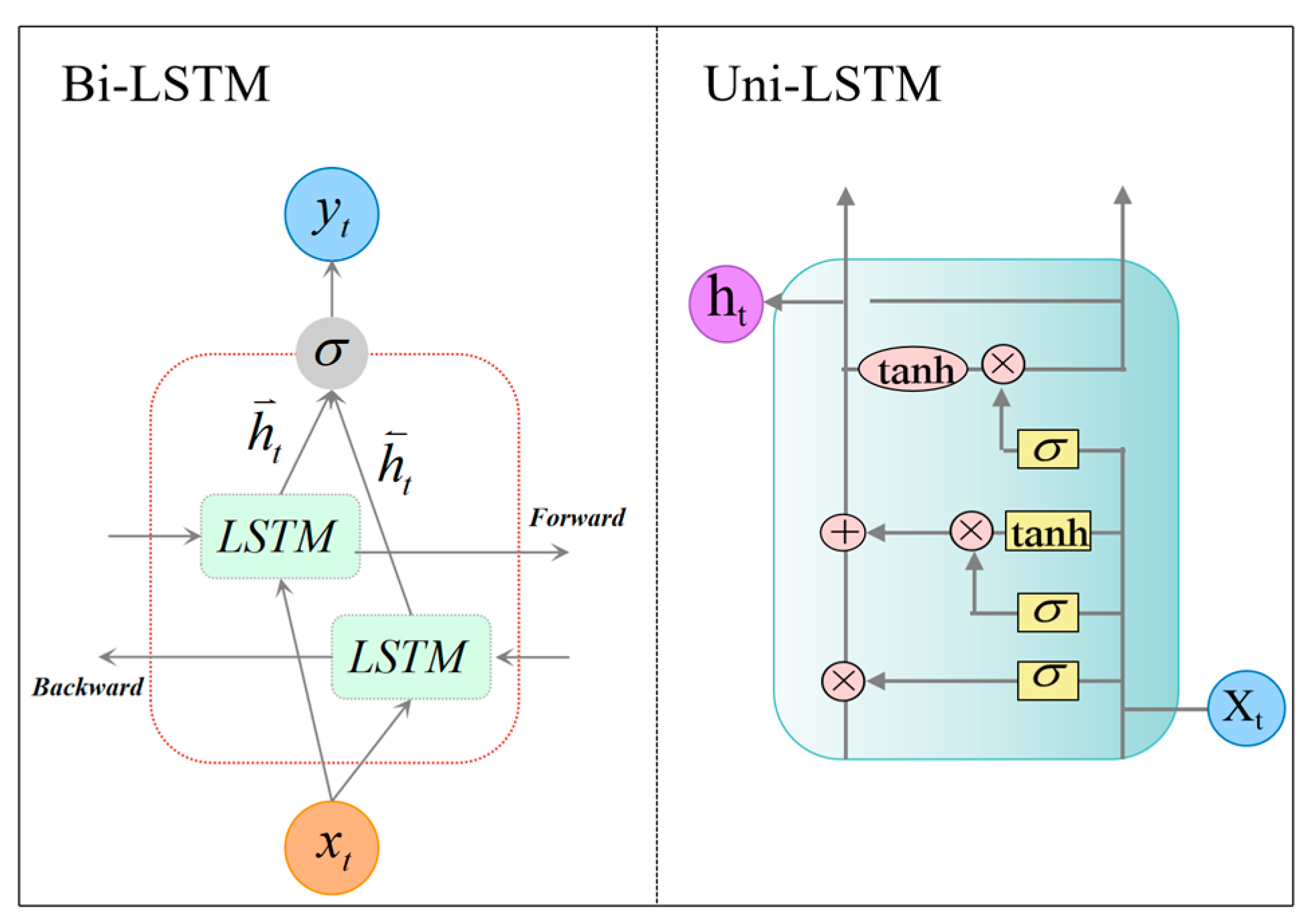
The Long Short-Term Memory network (LSTM) [31] is an improved architecture of Recurrent Neural Networks (RNN), effectively addressing the issues of vanishing and exploding gradients in long sequence training through the introduction of gating mechanisms. However, traditional LSTM models rely solely on past sequence states for information transmission, which limits their ability o accurately predict current or future states. To overcome this limitation, this study introduces a Bi–LSTM-based dual-channel LSTM architecture to enhance the model’s capacity for temporal feature extraction (see Figure 4). The data processed by the CNN is separately fed into two LSTM architectures: the main channel utilizes a two-layer bidirectional LSTM (with 64 hidden units and an input sequence length of 24) to capture forward and backward temporal dependencies and to model long-term trends, while the auxiliary channel adopts a three-layer unidirectional LSTM (with 32 hidden units) to strengthen the extraction of unidirectional patterns and to model short-term fluctuations. The outputs from both channels are concatenated along the feature dimension to form a 128-dimensional hybrid temporal feature vector, which is then used as input to the Transformer module.

2.3.3. Convolutional Neural Network

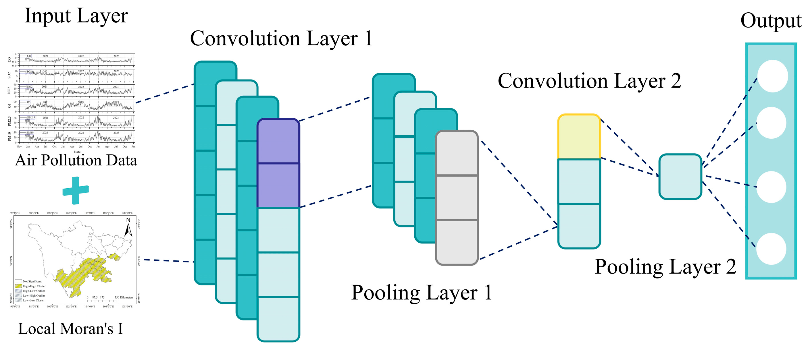
A Convolutional Neural Network (CNN) is a kind of feedforward neural network, which originated from Hubel and Wiesel’s research principle on biological visual cortex structure [32]. CNN network structure usually includes input layer, multiple convolution layers, pooling layer, fully connected layer and output layer [33], which has been widely used in image recognition and spatiotemporal sequence modeling because of its excellent spatial feature extraction ability. In this experimental framework, the input layer of CNN consists of two parts: one is the local Moran’s index (Moran’s I, the threshold is set to 0.3) calculated based on the latitude and longitude information of the observation site, and the other is the original observation data of the target pollutant. After the two are spliced, a data set with spatial autocorrelation characteristics is constructed, which is then input into convolutional neural network for feature extraction. Specifically, the model uses a convolutional layer with 64 filters (filter size = 5) to extract multivariate time series features, followed by a ReLU activation and a max-pooling layer to reduce feature dimensionality and capture key spatial patterns. The detailed process of the CNN module is shown in Figure 5.

2.3.4. Transformer Encoder

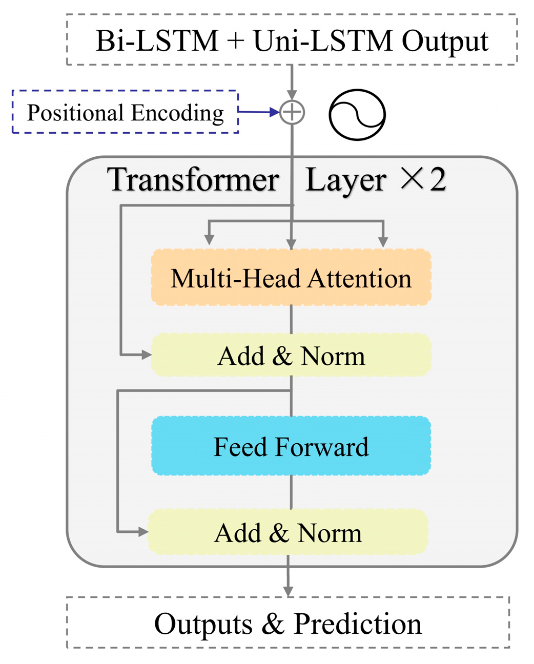
Transformer model is a deep neural network architecture built on the self-attention mec Transformer model is a deep neural network architecture based on self-attention mechanism, and its core advantage lies in breaking the strict dependence of traditional sequence modeling on time series calculation, and realizing efficient parallel computing and long-distance dependence modeling through global information interaction mechanism [34]. In order to enhance the modeling ability of the model to global features, this paper introduces the Transformer encoder module after CNN–LSTM structure. The module receives the LSTM output features processed by position coding, and uses two-layer Transformer encoder to model the global features. Each layer of encoder contains four self-attention heads, the feedforward network dimension is 256, the position coding dimension is set to 64, and the input channel is 128. At the same time, in order to enhance the dynamics of feature expression, the model designs a gating mechanism to adjust the feature intensity of Transformer output. Firstly, the 128-dimensional Transformer output is mapped to the weight vector of the same dimension, and the dynamic weight between 0 and 1 is generated after Sigmoid activation, which is used for weighted fusion of features. In the feature aggregation stage, the model averages the Transformer output in the time dimension to obtain the global context representation and extracts the features at the end of the sequence to represent the current state. The two are added and input to the fully connected layer for prediction. The detailed process of Transformer Encoder module is shown in Figure 6.

2.3.5. Bayesian Optimization

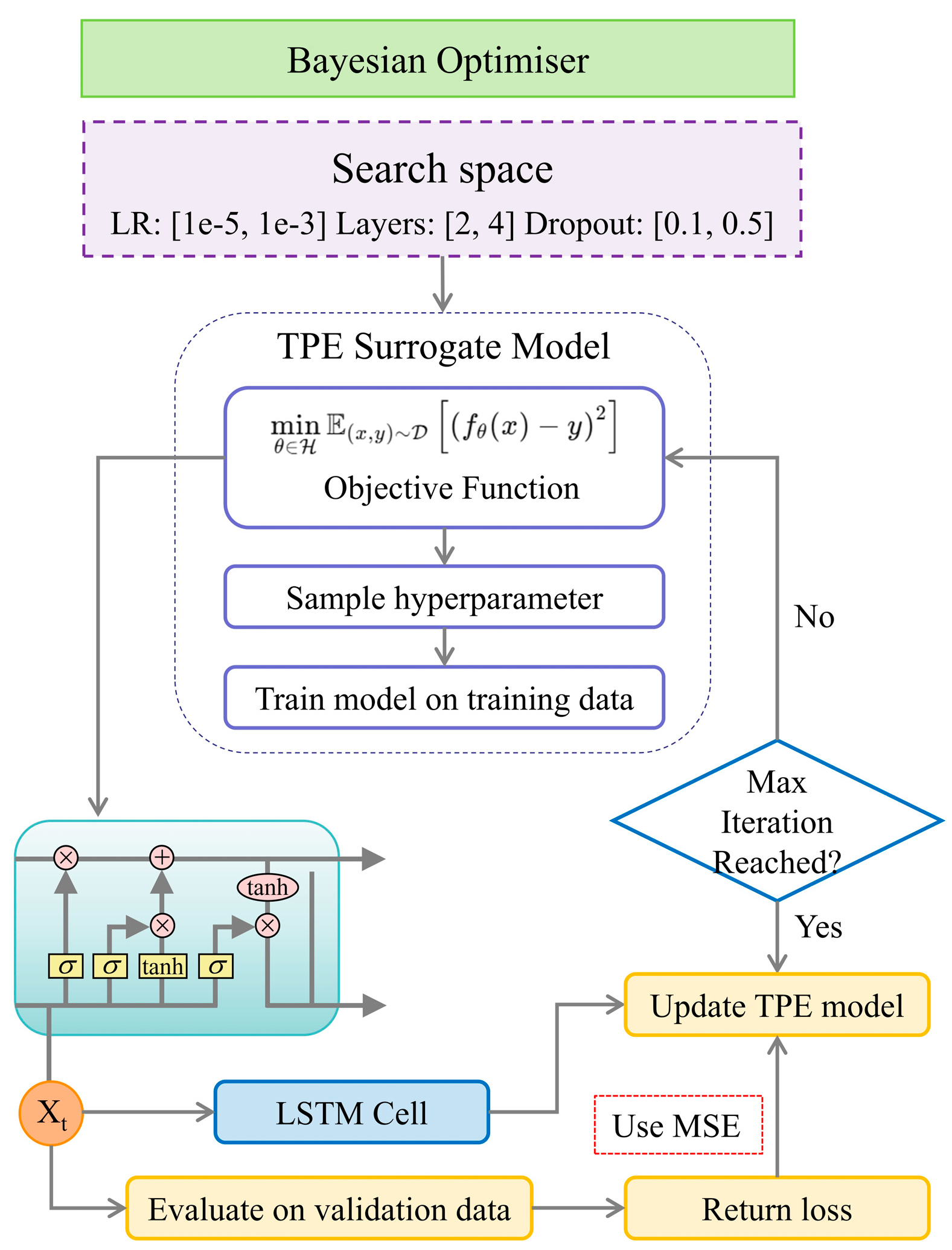
To enhance the dual-channel LSTM architecture’s ability to extract temporal features from time series data, Bayesian Optimization is used to automatically tune the key hyperparameters of the LSTM model [35], so as to improve the prediction performance and reduce human intervention. Bayesian optimization approximates the objective function by constructing a proxy model, balances exploration and utilization in each iteration, and selects the most promising parameter combination to improve the objective value. The goal of Bayesian optimization in this experiment is to minimize the mean square error on the verification set, that is
min θ H E ( x , y ) ~ D MSE f θ ( x ) , y
Here, θ represents the set of hyperparameters of the LSTM model, H denotes the hyperparameter search space, and fθ(x) is the model output trained with the hyperparameters θ.
The optimized three superparameters are: the learning rate (1−5–1−3), the number of LSTM layers (2–4) and the dropout rate (0.1–0.5). In this experiment, TPE (Tree-Structured Parzen Estimator) is used as a Bayesian optimization proxy model construction method, and it is bound to the objective function through the hyperopt.fmin interface. In order to reduce the computational cost, local Moran’s index (Local Moran’s I) is not introduced as an auxiliary feature in the Bayesian search stage for the time being, so as to ensure the controllability and quick response of the hyperparametric search process. The detailed process of Bayesian optimization module is shown in Figure 7.

3. Data Visualization Processing and Analysis

3.1. Time Evolution Characteristics Analysis

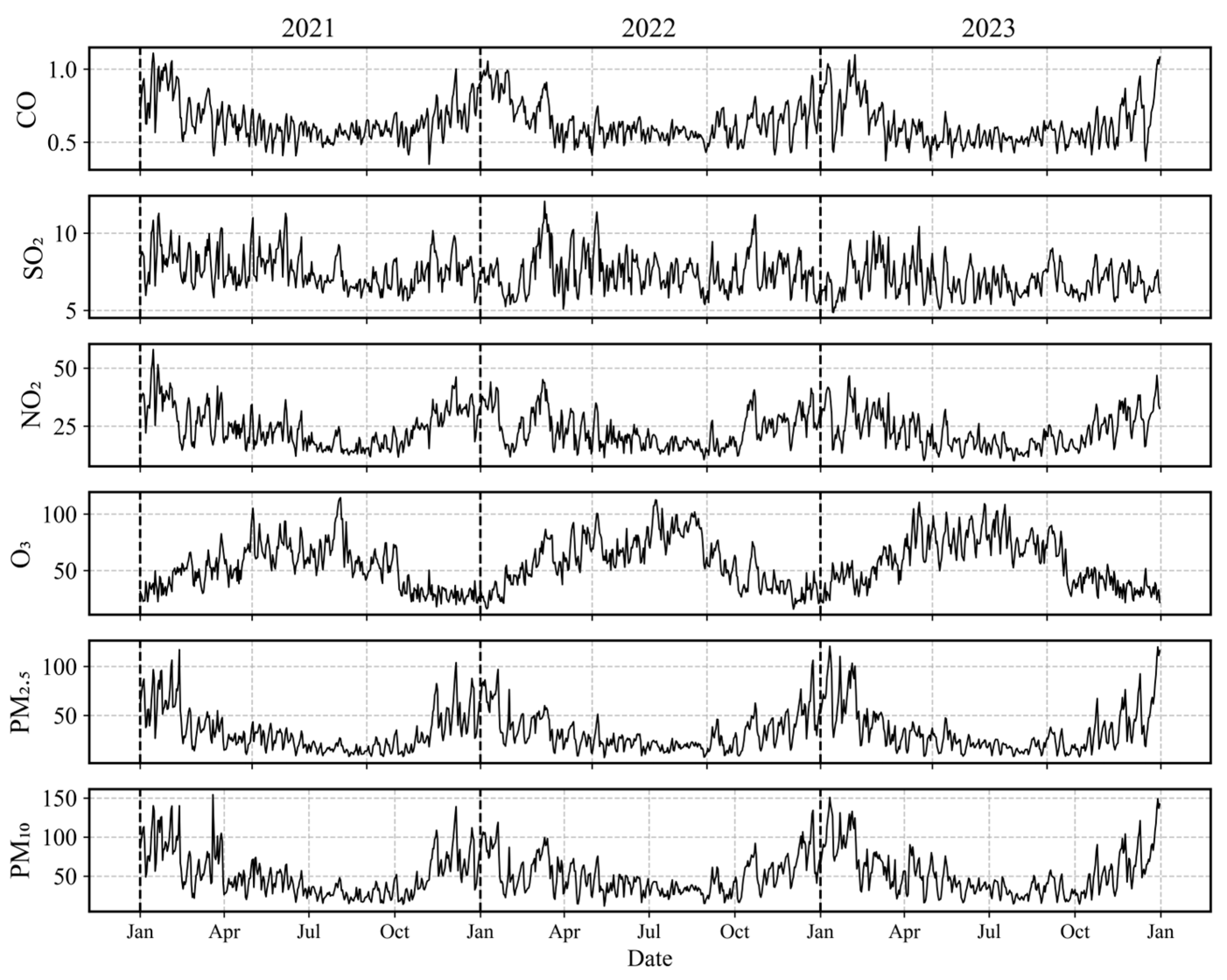
Based on the data of air pollutant reprocessing in Sichuan Province from 2021 to 2023, the daily average is calculated, and the three-year daily average line chart (Figure 8) and the annual average change comparison table (Table 3) are constructed.
According to the time-series distribution characteristics of pollutants, PM2.5 and PM10 concentrations show an obvious seasonal variation law, which is winter > spring > autumn > summer. NO2 and CO generally show the trend of winter > spring (or autumn) > summer; the time series characteristics of O3 are contrary to other pollutants, which are summer > spring > autumn > winter, showing typical photochemical pollution characteristics. However, SO2 did not show significant periodic fluctuation [36]. The above-mentioned temporal and spatial differences are mainly driven by the following factors: ① the frequent static weather in winter, the formation of the inversion layer, and the decrease in atmospheric boundary layer height constitute the “pot cover effect”, and the enhanced secondary organic aerosol generation leads to the enrichment of pollutants such as PM2.5, PM10, NO2 and CO near the ground; ② influenced by strong convective weather and precipitation in summer, pollutants can be effectively reduced through horizontal diffusion and wet deposition [37]; ③ the seasonal high value of O3 concentration is closely related to the enhancement of photochemical reaction intensity in summer, and its concentration is regulated by VOCs/NOₓ ratio, while the increase in O3 concentration in spring and autumn may be related to the increase in warm spring weather under the background of climate warming.
Further analysis of Table 3 shows that the annual average concentrations of CO, SO2 and NO2 have been continuously decreasing from 2021 to 2023: CO has decreased from 0.65 mg/m3 to 0.61 mg/m3 (cumulative decrease of 6.15%); SO2 decreased from 7.65 µg/m3 to 6.95 µg/m3 (a decrease of 9.15%); NO2 decreased from 24.55 µg/m3 to 22.62 µg/m3 (a decrease of 7.86%). This trend indicates that, since the enforcement of the 2015 Action Plan for Air Pollution Control, Sichuan Province has achieved notable reductions in emissions from conventional combustion sources through integrated industrial regulation, ultra-low emission upgrades, and the phase-out of coal-fired boilers. In contrast, O3, PM2.5, and PM10 show a “V” rebound trend: the annual average concentration of O3 increased from 127 µg/m3 (2021) to 136 µg/m3 (2023), with an increase of 7.09%; PM2.5 and PM10 rose by 2.53% and 3.08%, respectively. This phenomenon suggests that the regional compound air pollution control is facing new challenges against the background of the continuous decline of traditional pollutants, and it is necessary to further optimize the pollution collaborative control strategy.

3.2. Spatial Differentiation Analysis

3.2.1. Spatial Interpolation Method

In order to systematically reveal the spatial distribution characteristics of six air pollutants in 21 cities and states in Sichuan Province, Empirical Bayesian Kriging (EBK) was used to interpolate the discontinuous spatial observation data. The core reason for choosing this method was that 104 monitoring stations in the study area showed significant spatial cluster distribution characteristics. Traditional spatial interpolation methods are usually based on the assumption of spatial variability stationarity, that is, the spatial autocorrelation of the whole region is described by the global variation function, but this assumption faces significant challenges in the cluster distribution scene. For example, the Ordinary Kriging method needs to manually fit the variation function, and its process is easily influenced by the cluster distribution: the data points in dense areas dominate the fitting results, while the data contribution in sparse areas is systematically underestimated; although the Inverse Distance Weighting Method (IDW) relies on distance attenuation parameters, the cluster distribution makes the interpolation results of dense areas highly sensitive to parameter selection, while sparse areas are prone to “edge effect” due to the lack of adjacent points. These problems eventually lead to data redundancy in dense areas that may mask the real spatial gradient, while interpolation results in sparse areas are easily disturbed by outliers due to a lack of data. In contrast, the EBK method can automatically optimize key parameters such as the semivariogram through unique subset construction and an iterative simulation mechanism, thus effectively overcoming the modeling difficulties caused by spatial heterogeneity [38]. The core formula of this method can be expressed as:
Posterior prediction distribution: the posterior distribution of the predicted value ( Z ( s 0 ) ) of the observation points.
P ( Z ( s 0 ) | Z ) = P ( Z ( s 0 ) | θ , Z ) P ( θ | Z ) d θ
where P ( θ | Z ) P ( Z | θ ) P ( θ )   is the posterior distribution of hyperparameters and P ( θ )   is the prior distribution.
Prediction mean and variance: the Monte Carlo integral is used to approximate the posterior prediction.
Z ^ ( s 0 ) = 1 M m = 1 M λ ( m ) Z , σ 2 ( s 0 ) = 1 M m = 1 M C ( s 0 , s 0 | θ ( m ) ) λ ( m ) C ( m ) λ ( m )
where ( λ ( m ) = C ( m ) 1 c ( m ) ) , (c(m)) denotes the covariance vector between the unobserved location (s0) and the observed locations, (c(m)) represents the covariance matrix of the observed locations and represents a posterior sample of the model parameters.

3.2.2. Result

The interpolation results are shown in Figure 9, and the spatial distribution pattern shows significant spatial and temporal heterogeneity. In the figure, the row represents the interannual evolution trend of the same pollutant from 2021 to 2023, while the column shows the spatial interpolation results of the concentrations of six pollutants, namely O3, CO, NO2, PM2.5, PM10, and SO2, in sequence.
According to the types of pollutants, the area with high O concentration presents a “dual-core structure”: the main core area is distributed in the core urban agglomerations of Sichuan Basin (Chengdu, Deyang, Mianyang in Chengdu Plain Economic Zone and Zigong, Neijiang, Luzhou and Yibin in South Sichuan Industrial Zone) [39], and the secondary core area appears in the dry-hot valley of Jinsha River, such as Panzhihua. From the time evolution trend, the high-value area of CO show the characteristics of centripetal contraction, which covers Chengdu Plain, southern Sichuan and northeastern Sichuan in 2021. This gradually shrinks from northeastern Sichuan to the basin area in 2023, and the pollution range is also reduced, mainly in the Chengdu–Deyang–Mianyang industrial corridor, with an excellent pollution control effect. The combined pollution of NO2 and particulate matter presents a gradient distribution feature [40]: the high-value area of NO2 gradually converges from eastern Sichuan (2021) to the Chengdu Plain Economic Belt (2023), which is spatially coupled with the urbanization rate increased by 4.3 percentage points according to the data of the seventh population census; PM2.5 high-value nuclei exist stably in southern Sichuan industrial zone and Chengdu plain economic zone, and form stable pollution nuclei in the two places with the change of time [41]. However, the high value area of PM10 overlaps with the spatial pattern of NO2, and the concentration keeps increasing. SO2 pollution presents a pattern of “high in the south and low in the north”: South Sichuan industrial zone and Panxi area (Panzhihua and Liangshan) constitute the main high-value areas, which are closely related to the emissions of coal-fired industries. The SO2 concentration in Chengdu plain economic zone is relatively low, but there is still a certain high value near the industrial park. From 21 to 23 years, the concentration of SO2 decreased as a whole, and the high-value areas in southern Sichuan and Panxi decreased, indicating that the desulfurization treatment has achieved certain results.
From the overall trend, the regional comparative analysis shows that the Chengdu Plain Economic Zone, as a population-industry agglomeration center, has a significant concentration of NO2, PM2.5, PM10 and CO; due to the traditional industrial base, the South Sichuan Economic Zone has formed a high value of multi-pollutants, and the two regions together constitute the pollutant accumulation zone in the basin. The overall concentration in the Northeast Sichuan Economic Zone and Northwest Sichuan Plateau is low, but the second-highest value related to industrial/motor vehicle emissions appears locally. Due to the characteristics of resource-based industries in the Panxi Economic Zone, SO2 and CO present discrete high values, but the pollution range is limited. Most pollutants in the mountainous areas of northwest Sichuan maintain a background level, and only high values appear around the mining area.

3.3. Analysis of Interrelationships Among Pollutants

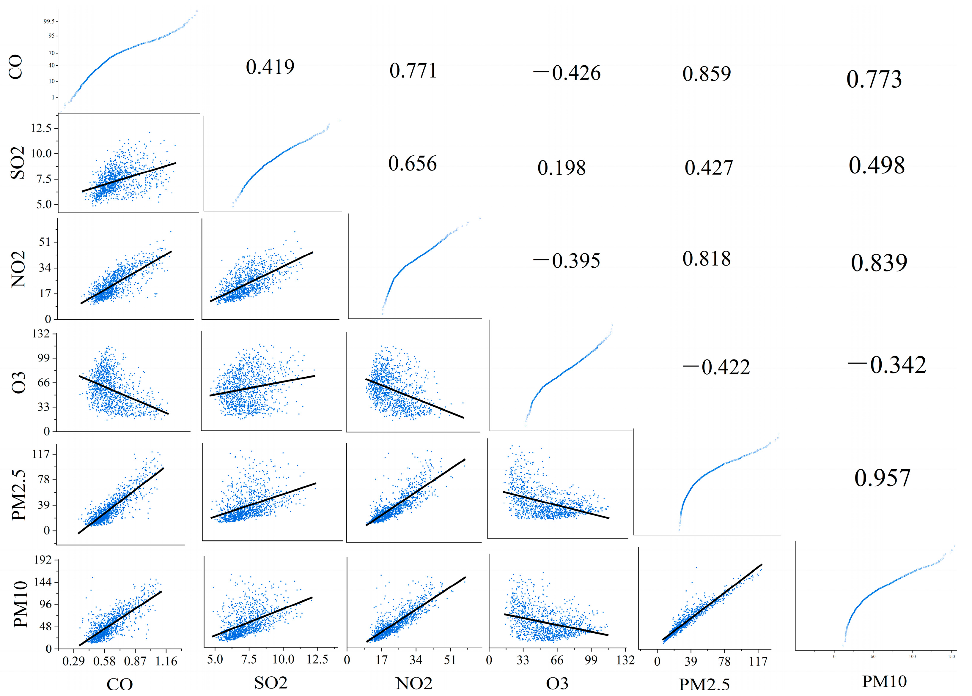
Based on the reprocessed data, the daily average of six air pollutants in the Sichuan Province from 2021 to 2023 is calculated, the Pearson correlation coefficient is analyzed, and Figure 10 is drawn. The lower left corner and the upper right corner of the figure are the scatter plot and correlation values between pollutants, respectively, and the central axis is the numerical probability distribution of the corresponding pollutants. According to the analysis, the inter-pollutant correlations can be broadly categorized into the following three dimensions:
(1)
Strong synergistic effect of homologous pollutants:
CO, NO2, PM2.5 are positively correlated with PM10 (r = 0.771–0.957), and their synergy comes from the co-emission mechanism: ① motor vehicle exhaust (diesel/gasoline vehicle) and incomplete combustion process of coal-fired boiler simultaneously release CO, NOx(NO2 precursor) and particulate matter; ② coal-fired heating in winter strengthens the synchronous accumulation of CO and particulate matter (PM2.5/PM10), while traffic source emissions drive the spatiotemporal coupling of NO2 and PM2.5. In addition, nitrate (accounting for 15–30% of PM2.5) generated by photochemical conversion of NOx and the synergistic effect of elevated CO concentration on particulate matter accumulation under static meteorological conditions further strengthen the correlation of this pollution cluster [42].
(2)
Compound action chain of sulfur-containing pollutants:
SO2 exhibits a moderate positive correlation with CO, NO2, and PM2.5 (r = 0.419–0.656), attributable to two main mechanisms: ① the concomitant of primary emission—the simultaneous release of SO2 and NOx by the combustion of sulfur-containing fuel (coal/heavy oil) [43], especially in the energy structure of Sichuan, where coal accounts for over 60%; ② secondary transformation path—SO2 is oxidized in the atmosphere to generate sulfate (accounting for 20–35% of the secondary component of PM2.5), while PM10 is mainly from primary emissions such as dust, and has weak correlation with SO2. This difference confirms the dominant position of secondary transformation in the formation of fine particles.
(3)
Dynamic Antagonism Between Ozone and Primary Pollutants:
O3 is negatively correlated with CO, NO2, and PM2.5 [44] [r = (−0.395)–(−0.426)], and this relationship is shaped by both spatiotemporal divergence and chemical inhibition: ① seasonal complementarity—O3 the summer peak of O3 (strong radiation/high temperature) and the accumulation of CO/PM2.5 under the inversion layer in winter form anti-phase fluctuation; ② photochemical inhibition chain: NOx titration effect (NO + O3 → NO3 + O3) consumes O3 significantly in traffic-dense areas, and the radiation scattering of PM2.5/PM10 reduces the photolysis rate J [NO2] by 30–50%, while the excess of NOx (VOCs/NOx < 4) associated with high PM environment makes O3 production limited by volatile organic compounds. This multi-scale coupling mechanism reveals the nonlinear characteristics of “gas–particle” interaction in compound pollution.
To sum up, based on the correlation analysis, there is an obvious correlation among the six pollutants. The most obvious is the strong synergistic correlation (r = 0.771–0.957) between homologous pollutants (CO, NOx, PM, and SO2). Secondly, SO2 has a moderate positive correlation with CO, NO2, and PM2.5 (r = 0.419–0.656), and O3 has a negative correlation with primary pollutants (CO, NO, PM2.5) (r = −0.395–0.426). The above-mentioned multi-dimensional correlation characteristics show that when building an air pollution prediction model, it is necessary to systematically integrate the synergistic/antagonistic relationship between pollutants, extract the influence weight distribution between different pollutants, and optimize the prediction results of the model according to the interaction mechanism between pollutants in different seasons.

4. Experiments

4.1. Evaluation Metrics and Training Strategy

4.1.1. Evaluation Metrics

In order to comprehensively evaluate the prediction accuracy of the integrated model, MAE (mean absolute error), RMSE (root mean square error) and R2 (determination coefficient) are used as performance evaluation indicators [45], which are used to quantify the average deviation between the predicted value and the actual observed value, reflect the dispersion degree of the predicted results and characterize the model’s ability to explain the variation law of pollutant concentration. The calculation formula is as follows:
M A E = 1 n i = 1 n y i y ^ i
RMSE = MAE = 1 n i = 1 n ( y i y ^ i ) 2
R 2 = 1 SSE SST = 1 i = 1 n ( y i y ^ i ) 2 i = 1 n ( y i y ¯ ) 2
where y i and y ^ i denote the observed and predicted values, respectively, y ¯ is the mean of the observed values, and n represents the total number of samples.

4.1.2. Training Strategy

In the process of parameter optimization and training of the integrated model, the urban air pollution observation data set is divided into a training set, a verification set and a test set according to the time sequence in the ratio of 0.75:0.15:0.15. At the same time, in both stages, the training strategy of early stop triggered by the loss of 10 epochs in the verification set is set to ensure the balance between convergence stability and computational efficiency.
In the process of Bayesian optimization of the super-parameter of the LSTM model, the optimized four super-parameters and their value ranges are: the learning rate (1−5–1−3), the number of LSTM layers (2–4) and the dropout rate (0.1–0.5). Each round of hyperparametric combination will be used to train an LSTM model. During the training process, at most 40 epochs will be iterated, and the EarlyStopping strategy will be adopted to avoid over-fitting. The model takes MSE (Mean Square Error) as the loss function to evaluate the performance. Bayesian optimization algorithm uses TPE strategy, constructs a posterior probability distribution according to the currently observed performance, and selects the next group of super-parameter combinations, which are more promising to obtain low loss. The optimization process is carried out for 30 iterations to find the optimal super-parameter configuration.
In the CNN–LSTM–Transformer model, the pollutant concentration prediction task uses a sliding time window to construct the input sequence. According to the different forecasting tasks, the model has two input and output forms: single-step forecasting and multi-step forecasting. In the single-step forecasting, the model takes multi-feature data of seven consecutive days as input to predict the target pollutant concentration on the eighth day. In the multi-step prediction, the input window is extended to 9 days, and the output is the pollutant concentration series of the next 1–4 days, in order to test the prediction ability of the model under a continuous time step. The input features of the model include six common air pollutants (CO, PM10, PM2.5, SO2, NO2, and O3) and the Local Moran’s Index, with a univariate prediction framework, that is, only the future concentration of one target pollutant is predicted at a time. During the training process, the model iteration period (epoch) is set to 100, and the batch size is 32. The key hyperparameters of the LSTM module (such as hidden layer dimension, network layer number, dropout ratio and learning rate) are automatically searched by the Bayesian optimization method, thus improving the model performance and enhancing the generalization ability. The specific structural designs of CNN, LSTM and Transformer in the model are detailed in Section 2.3.2, Section 2.3.3 and Section 2.3.4 and their static parameter configurations are detailed in Table 4.

4.2. Experimental Results

4.2.1. Selection of Benchmark Cities

To validate the effectiveness of the proposed model in predicting air pollutant concentrations, Chengdu, a representative and typical city within the study area, is selected as the benchmark city. Accordingly, the analyses in Section 4.2.2, Section 4.2.3 and Section 4.2.4 are all conducted using Chengdu as the basis for analysis. The reason for choosing Chengdu as the benchmark city is as follows:
First of all, from the representative point of view of compound pollution sources, Chengdu, as the first city in Sichuan Province, has a concentrated 25.67% of its permanent population and 39.43% of its motor vehicle ownership [46]. Its pollution source structure has typical composite characteristics: industrial emissions are important pollution sources, among which steel and chemical industries are more prominent. By September 2024, the NOx and VOCs emitted by mobile sources brought by 6.852 million motor vehicles in Chengdu accounted for 85% and 40% of the city’s emissions, respectively. In addition, the sources of dust and life can not be ignored. This multi-source coexistence pollution pattern is differentiated and complementary with basin cities such as Mianyang, which accounts for 41.66% of the industry, and Deyang, which is dominated by heavy industry and can fully reflect the regional pollution characteristic pedigree.
Secondly, from the perspective of a typical diffusion mechanism under topographic constraints, Chengdu is located at the “bowl bottom” of Sichuan Basin, with Longmen Mountain (750–4989 m above sea level) in the west and Longquan Mountain (500–1046 m above sea level) in the east, forming a semi-closed topographic unit. Meteorological observation data show that the average annual quiet wind frequency in this area is 32~55%, and the inversion layer appears frequently. Under the condition of a specific wind direction, industrial emissions from surrounding cities can be transported to the main urban area of Chengdu and accumulated. This coupling mechanism of “regional transport–local accumulation” has obvious isomorphism with basin cities such as Nanchong and Luzhou. Through the observation data in Chengdu, it can be indirectly verified that the model can capture the regional transmission process.
This multi-dimensional typicality makes Chengdu an ideal case for studying the spatiotemporal evolution of air pollution in the Sichuan Basin, and the underlying mechanisms identified here can partially reflect pollution trends across other regions of the province. Additionally, the diffusion parameters and meteorological coupling relationships validated by the model in Chengdu can be partially extrapolated to urban agglomerations in the northern hilly areas of the Sichuan Basin and the industrial cities of southern Sichuan—such as Nanchong and Mianyang—which share similar topographical and geomorphological features with Chengdu, and Yibin and Luzhou, which exhibit comparable industrial structures.

4.2.2. Comparative Experiments

To verify the performance of the proposed model, this paper selects five mainstream deep learning models as comparison objects, covering parameter optimization and structural integration methods that demonstrate strong representativeness and broad applicability. These models can be divided into two categories: parameter optimization-based models, including BO–LSTM [47], WOA–LSTM [48], BO–CNN–LSTM [49], and WOA–CNN–LSTM [23];, while the model integration method is represented by CNN–LSTM [24]. In addition, to further evaluate the roles of CNN, Bayesian optimization, and Local Moran’s Index in the integrated model, we also constructed ablation models including CNN–LSTM–Transformer, BO–LSTM–Transformer, and BO–CNN–LSTM–Transformer without LMI features.
Specifically, CNN–LSTM serves as a classical fusion model that has been widely applied in forecasting tasks by jointly extracting temporal and spatial features. In this study, this model serves as the baseline for an integrated structure to verify its generalization ability in the complex geographical environment of Sichuan Province. Moreover, BO–LSTM, WOA–LSTM, BO–CNN–LSTM, and WOA–CNN–LSTM represent integrated models for hyperparameter tuning based on traditional LSTM and CNN–LSTM structures, respectively. These four models are used to test the improvement effects of different hyperparameter optimization algorithms on model performance and to determine the optimal parameter optimization algorithm. To further verify the effectiveness of key modules in the proposed framework, this paper designs three groups of ablation experiments that analyze the optimization algorithm, spatial feature extraction module, and spatial dependency modeling features, respectively. First, we construct a CNN–LSTM–Transformer model without the Bayesian optimization (BO) process to evaluate BO’s performance improvement effect in hyperparameter tuning. Second, we build a variant model (BO–LSTM–Transformer) that removes the CNN module while retaining only LSTM and Transformer structures to examine CNN’s role in capturing spatiotemporal coupling features. Finally, we construct a BO–CNN–LSTM–Transformer model without Local Moran’s Index (LMI) features to test whether this spatial autocorrelation feature contributes significantly to model performance.
Table 5 presents the performance of nine models in predicting concentrations of six atmospheric pollutants in Chengdu. In terms of mean absolute error (MAE), the proposed integrated model (BO–CNN–LSTM–Transformer) achieves optimal performance across all pollutant predictions. Compared to the second-best models, this model reduces MAE by 17.9%, 13.7%, 18.2%, 19.6%, 2.3%, and 5.0% for CO, PM10, PM2.5, NO2, SO2, and O3, respectively. In most cases, the second-best models are CNN–LSTM–Transformer or BO–CNN–LSTM–Transformer without LMI. Regarding root mean square error (RMSE), the integrated model also demonstrates optimal performance for CO, PM10, PM2.5, NO2, and O3 predictions, with reductions of 9.0%, 11.6%, 25.5%, 6.9%, and 0.9% compared to second-best models, respectively. For SO2 prediction, its RMSE is slightly higher than BO–LSTM–Transformer (10.29 vs. 10.76), but the difference is minimal. In terms of the coefficient of determination (R2), the integrated model achieves the highest scores across all pollutants: 0.878 (CO), 0.884 (PM10), 0.873 (PM2.5), 0.894 (NO2), 0.874 (SO2), and 0.883 (O3). Compared to second-best models, R2 improvements range from 1.5% to 7.4%, indicating that the model not only possesses strong fitting capability but also maintains good generalization performance across different pollutant types.
The comprehensive results across three indicators show that BO–LSTM and WOA–LSTM models exhibit relatively weak overall performance. Although parameter optimization methods improve LSTM prediction accuracy to some extent, they struggle to accurately model pollution distribution characteristics in areas with obvious spatial pollution concentration, such as the Sichuan Basin, because they rely solely on time series information without considering spatial neighbor correlations. However, CNN–LSTM, BO–CNN–LSTM, and WOA–CNN–LSTM, which further introduce local spatial feature extraction capabilities, perform better than the former models, verifying the importance of convolution modules in extracting local spatial patterns and capturing pollution clustering. Among these, BO–CNN–LSTM generally outperforms WOA–CNN–LSTM, further reflecting the higher efficiency and stability of Bayesian optimization in LSTM hyperparameter tuning.
The integrated model and three ablation experiments demonstrate that the proposed integrated model significantly outperforms other models across multiple pollutants, with advantages stemming from synergistic effects between sub-modules. Specifically, after removing the Bayesian optimization module (CNN–LSTM–Transformer), the model shows decreased prediction accuracy for most pollutants, indicating that Bayesian algorithms enhance overall performance stability through automatic hyperparameter adjustment. In contrast, the BO–LSTM–Transformer model without CNN modules shows more pronounced performance degradation for spatially heterogeneous pollutants such as PM10 and NO2, verifying the critical role of CNN structures in extracting local spatial features. When Local Moran’s Index (LMI) features are removed (BO–CNN–LSTM–Transformer without LMI), the model shows significant R2 decreases for pollutants such as O3 and NO2, indicating that LMI, as a spatial autocorrelation measure, effectively enhances the model’s perception capability for complex terrain and local pollution clustering areas. The comparative results of the three ablation models collectively confirm the irreplaceable role of each sub-module in modeling spatial and temporal characteristics of different pollutants, further explaining the integrated model’s stable and superior prediction performance across multiple pollutants and indicators.
Generally speaking, although the integrated model occasionally shows slightly lower MAE or RMSE values than some optimal models for individual pollutants, it consistently maintains leadership in R2 values, demonstrating remarkable advantages in overall fitting accuracy and generalization ability while verifying its effectiveness and robustness in complex regional pollution prediction tasks.

4.2.3. Comparison and Error Analysis of PM2.5 Prediction Models

Considering the representativeness of different models in structural characteristics and prediction performance, this section selects seven core models as comparison objects: BO–LSTM, WOA–LSTM, CNN–LSTM, BO–CNN–LSTM, WOA–CNN–LSTM, CNN–LSTM–Transformer, and BO–CNN–LSTM–Transformer. Although this study also constructed two ablation models (BO–LSTM–Transformer and BO–CNN–LSTM–Transformer without LMI), their overall prediction indicators show minimal differences from other main models, making it difficult to demonstrate more distinguishable comparative effects in visualization dimensions such as trend fitting and error distribution. To ensure clarity and representativeness in graphical analysis, subsequent visualization experiments are uniformly based on the aforementioned seven models.
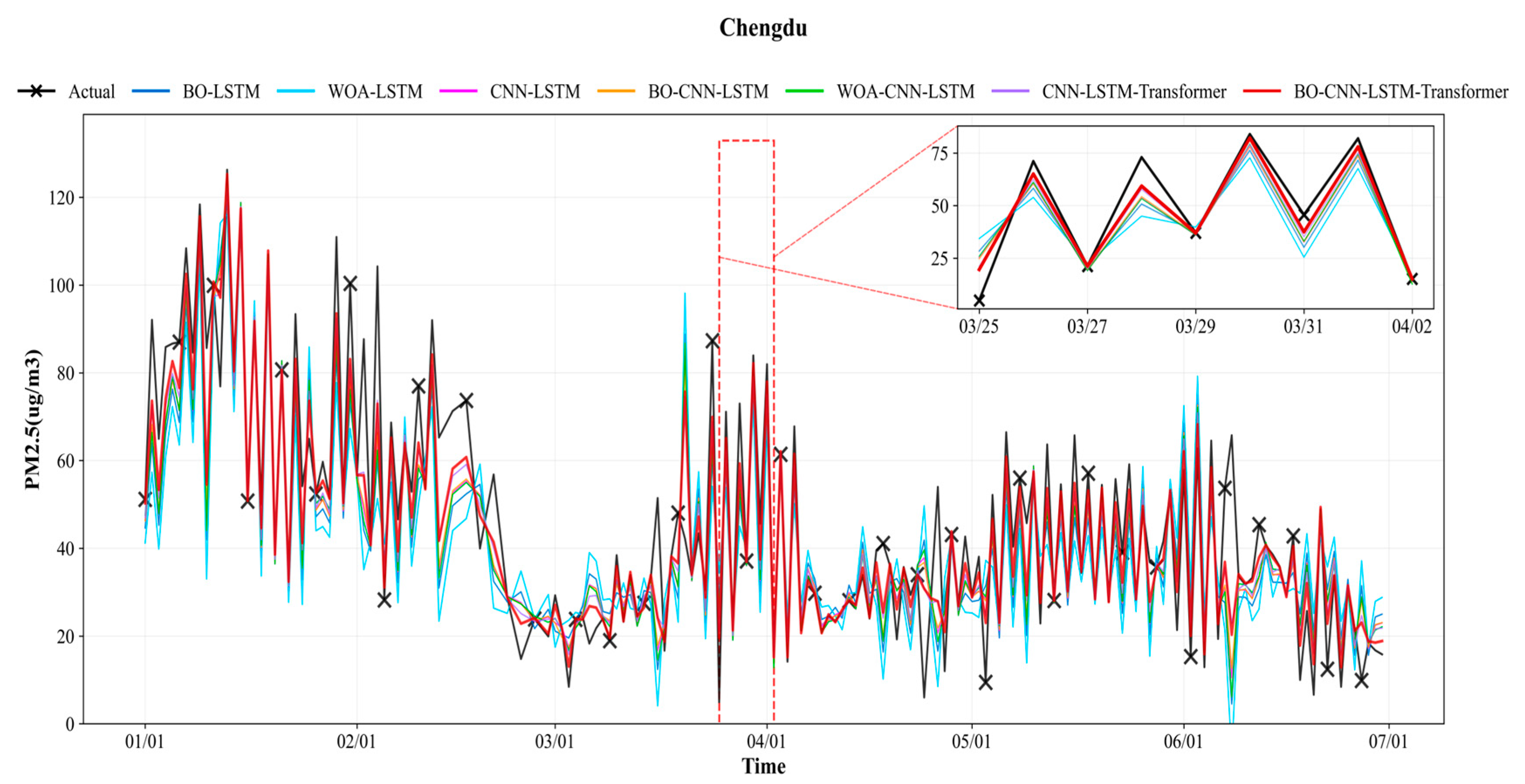
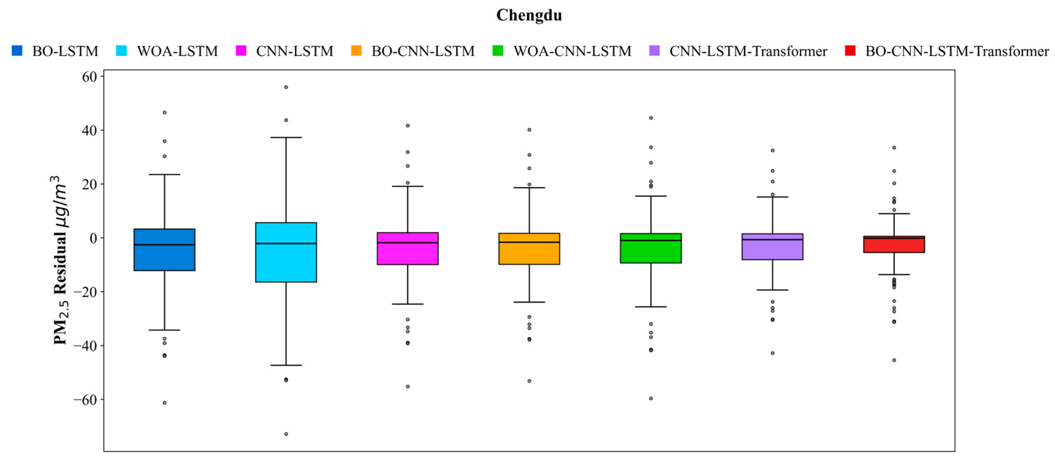
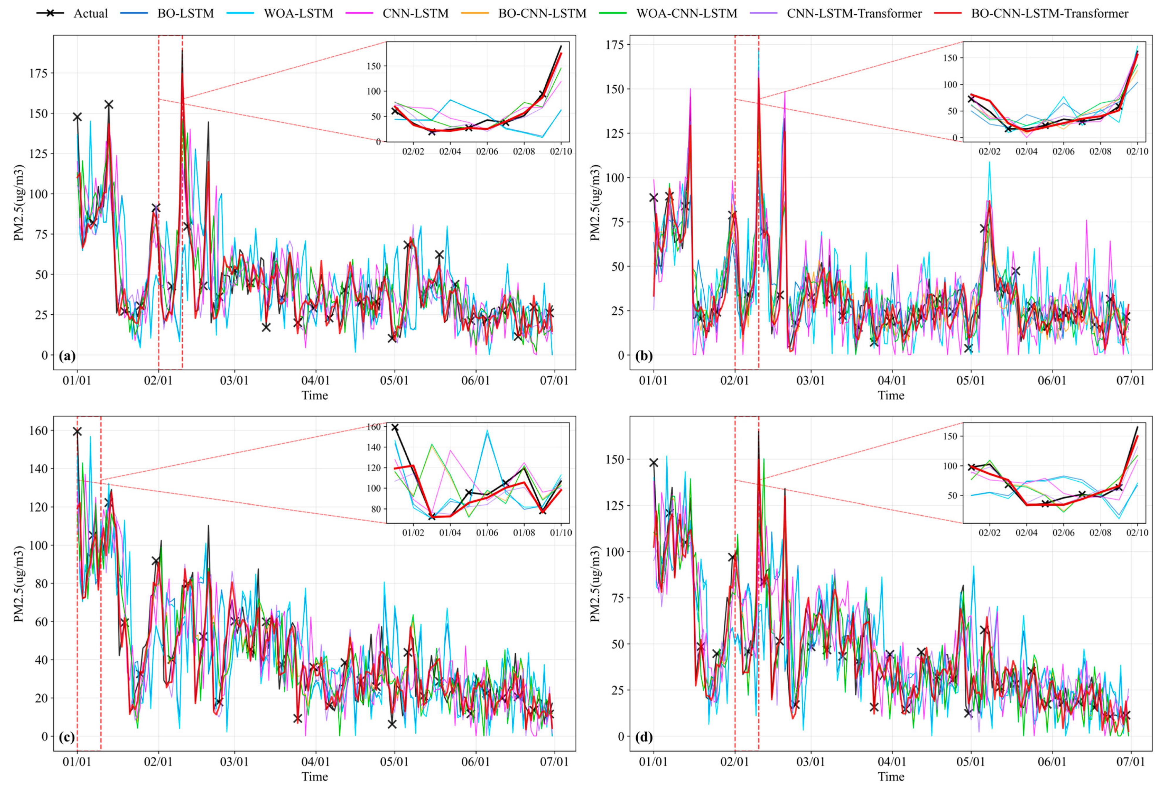
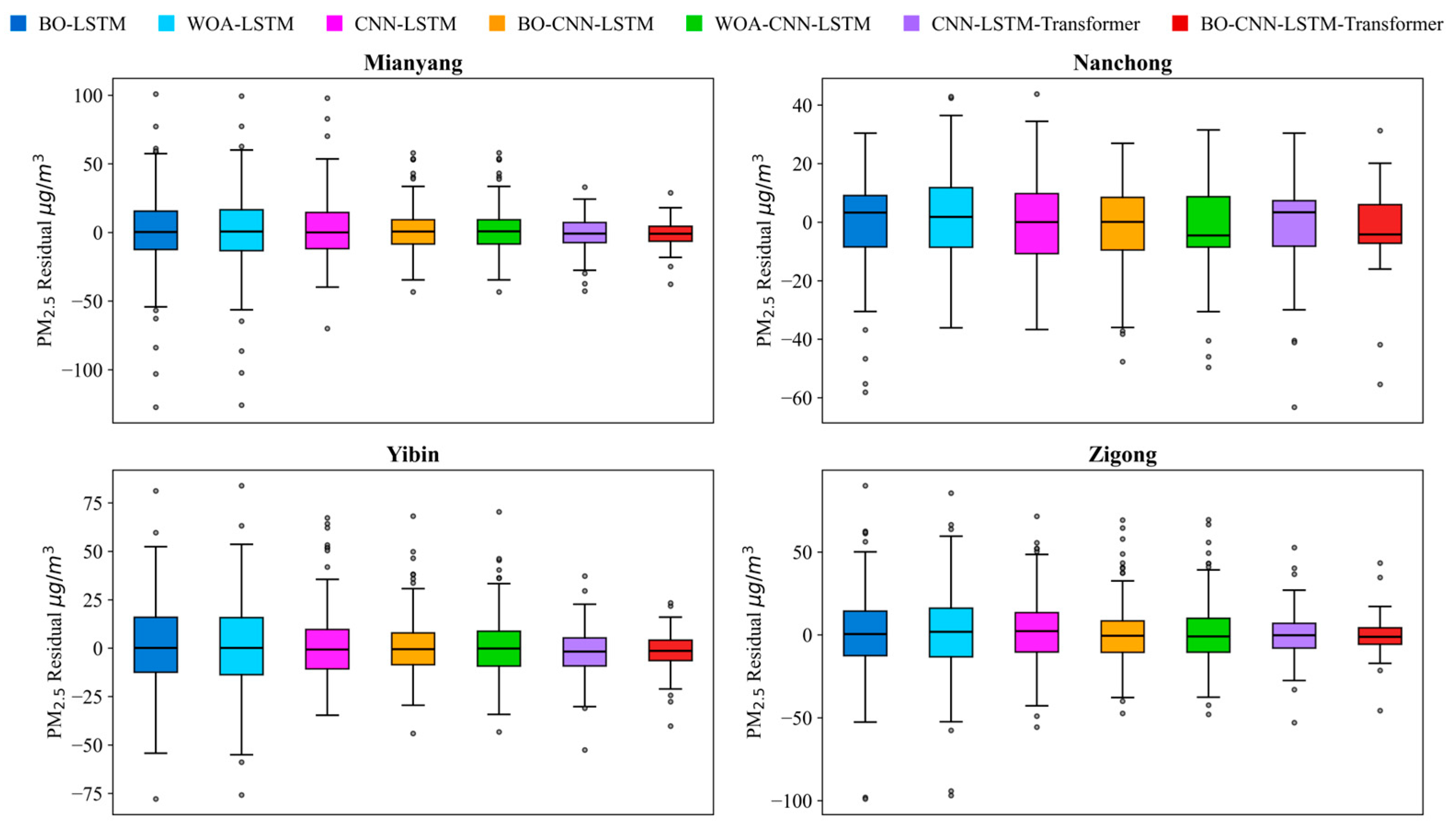
To comprehensively evaluate the performance of each model in the PM2.5 single-step prediction task, Figure 11 and Figure 12 present a comparison of the seven models from two dimensions: Figure 11 shows the fitting curves between the predicted and observed values to assess each model’s ability to reproduce trends; Figure 12 uses residual boxplots to display the distribution characteristics of prediction errors, reflecting the model’s stability and bias control. PM2.5 is chosen as the main focus for visualization because, according to the statistical results of pollution days exceeding the secondary limits of the Environmental Air Quality Standard (GB 3095-2012) [50] shown in Table 6, between 2021 and 2023, days with PM2.5 exceedances accounted for 62.6% to 83.5% of all pollution exceedance days, making PM2.5 the primary factor in the air quality decline in Chengdu. Therefore, focusing on PM2.5 prediction results has strong representativeness and practical significance.
From Figure 11, it can be observed that most models generally capture the overall trend of PM2.5 in the single-step prediction task, fitting the temporal fluctuations of PM2.5 relatively well. However, differences in fitting accuracy among models become more apparent during periods of rapid increases or decreases in pollution concentration (such as in January 2024 and from late March to early April). Specifically, traditional architectures like BO–LSTM and WOA–LSTM exhibit obvious lag in responding to extreme values; especially around pollution peaks, their predicted fluctuations are less intense than the actual values, resulting in a “peak shaving and valley filling” effect. In contrast, CNN–LSTM and its optimized versions that incorporate convolutional structures show stronger capability in capturing local variations, with prediction curves closely following the true changes during these volatile periods, indicating that the CNN architecture helps enhance short-term local feature extraction.
The comparison of residual distributions in Figure 12 further supports the above analysis. The WOA–LSTM model exhibits the largest residual fluctuations with numerous outliers, indicating highly unstable errors. Although BO–LSTM shows some improvement, it still suffers from error accumulation due to the limitations of the single-channel LSTM structure when handling complex temporal disturbances. This suggests that both single-channel LSTM-based models are prone to accumulating errors under complicated time-series variations. In contrast, the introduction of CNN structures (such as CNN–LSTM and BO–CNN–LSTM) effectively enhances the model’s ability to extract local features, resulting in more concentrated residuals and fewer outliers. Furthermore, the CNN–LSTM–Transformer model and the integrated model (BO–CNN–LSTM–Transformer) perform best in both figures: their prediction curves closely overlap with the actual values, showing significantly better trend consistency than other models. Their residual distributions are also the most compact, with mean and median values near zero and almost no significant bias, along with the fewest outliers. This reflects the model’s strong stability and robustness in the prediction task. Notably, the integrated model excels at controlling error propagation over long time steps, demonstrating the synergistic effects of structural integration and hyperparameter optimization.
Based on the analysis results of the two graphs, it can be seen that both the integrated model and CNN–LSTM–Transformer model have leading advantages in the single-step prediction task. The integrated model not only improves the accuracy of multi-step prediction, but also effectively reduces the systematic deviation and extreme error fluctuation, showing the strongest generalization ability and engineering application potential by integrating CNN, dual-channel LSTM and Transformer modules and introducing Bayesian optimization strategy.

4.2.4. Multi-Step Forecasting Evaluation

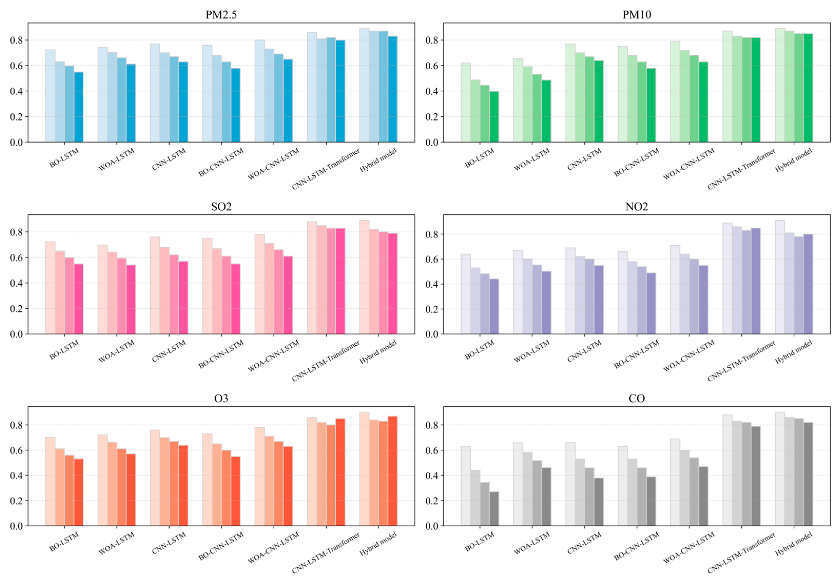
In the multi-step prediction task, the model’s performance gradually decreases with the increase in prediction step size. In order to evaluate the fitting ability of each model to the trend change of pollutants more comprehensively, this paper selects the determination coefficient (R2) as the main evaluation index to compare the multi-step prediction performance. The reason is that, compared with the error indicators such as MAE and RMSE, R2 can comprehensively reflect the fitting ability of the model to the fluctuation trend of the target variable in long-time series prediction, and its numerical fluctuation can sensitively reveal the generalization stability of the model in different time steps [51]. Therefore, in this paper, the R2 variation range (maximum and minimum) of the prediction results of six kinds of pollutants on the fourth day, compared with the prediction results on the first day of each model, is used as the comparison standard of model stability. At the same time, to verify the robustness of the comparison results, the mean absolute error (MAE) and root mean square error (RMSE) comparison results are provided below to comprehensively reflect the differences in model accuracy and fitting ability.
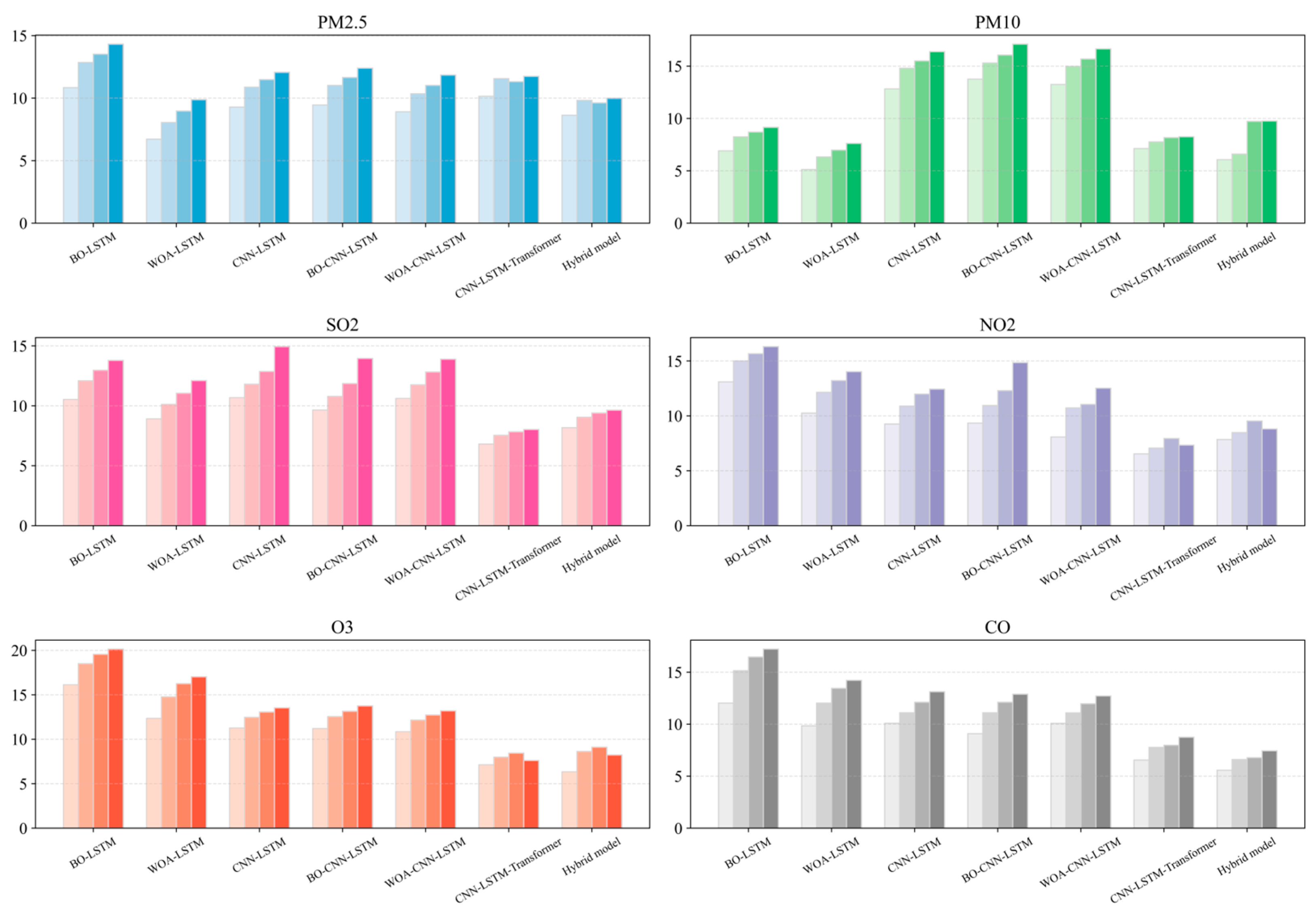
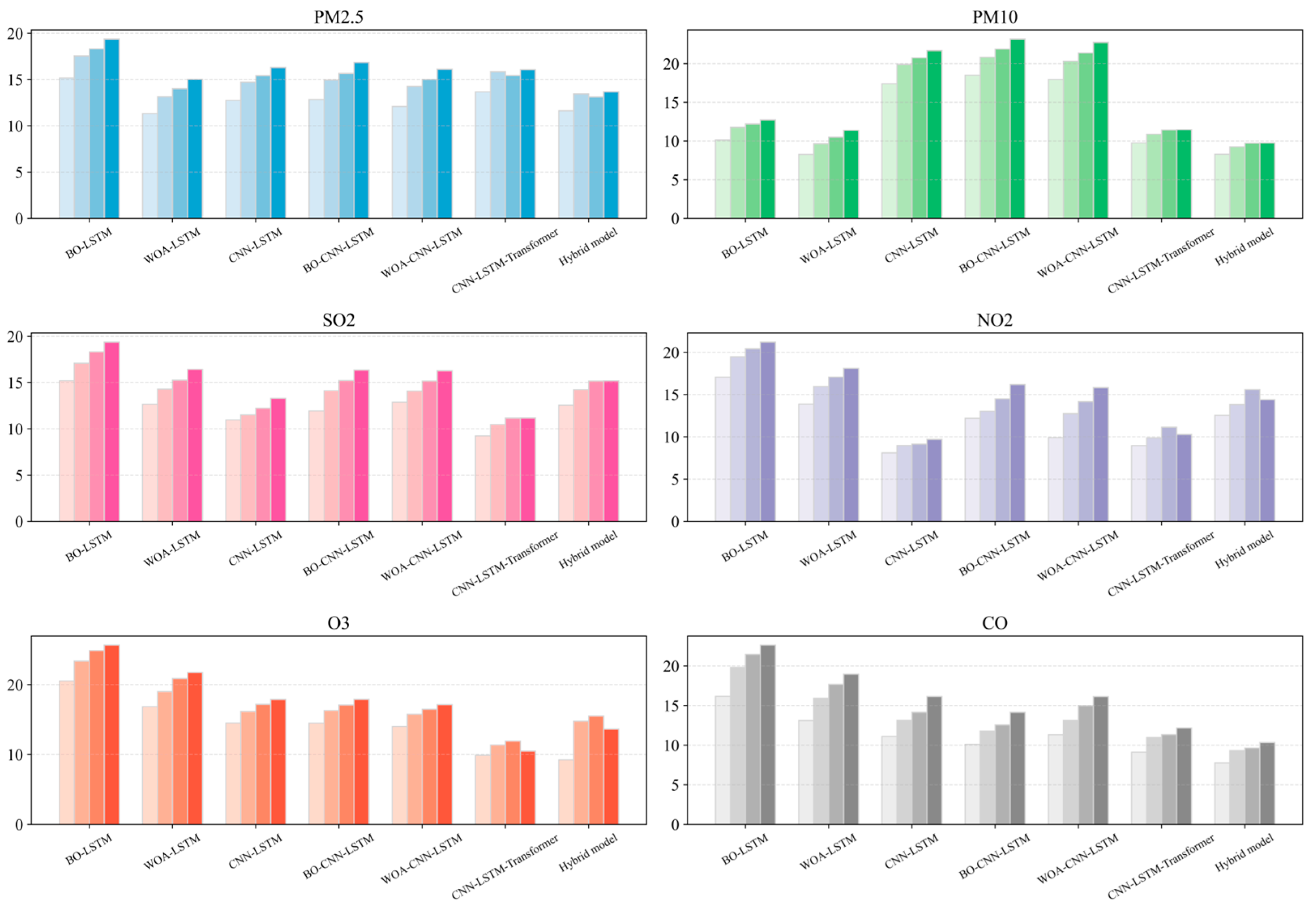
Figure 13, Figure 14 and Figure 15 show the changes of MAE, RMSE and R indicators of BO–LSTM, WOA–LSTM, CNN–LSTM, WOA–CNN–LSTM, BO–CNN–LSTM, CNN–LSTM–Transformer and the integrated model in the 1–4-day forecasting task, respectively, in which the histogram color from shallow to deep represents the increase in the forecasting time step from 1 to 4 days.
The results shown in the figures reveal significant differences among models in terms of performance decline and metric behavior, with an overall trend of decreasing prediction accuracy as the forecast horizon lengthens. Regarding the stability of the R2 metric, single LSTM architectures such as BO–LSTM and WOA–LSTM exhibit substantial accuracy drops in multi-step prediction, with R2 changes ranging from −24.1% to −56.9% and −30.1% to −40.2%, respectively, indicating considerable error accumulation in modeling long-term dependencies. CNN–LSTM and its hyperparameter-optimized versions show some improvement in R2 decline, but fluctuations remain significant at (−18.2% to −42.4%), (−22.7% to −38.1%), and (−18.8% to −31.9%). In contrast, the CNN–LSTM–Transformer model and the integrated model demonstrate much narrower R2 fluctuations, ranging from −1.16% to −10.23% and −6.7% to −12.4%, respectively, representing a 4 to 6 times reduction in variability compared to the worst-performing models and indicating stronger stability in multi-step prediction.
Further analysis shows that the reason why CNN–LSTM–Transformer model is superior to the integrated model in numerical change is that the integrated model uses a Bayesian optimization (BO) mechanism to optimize the first-day parameters, which shows better results in the first-day prediction. However, due to the same parameters as the first day, some parameters of the subsequent step drift, which is quite different from the results of the first day, so the change range is greater than that of the CNN–LSTM–Transformer model. The reason for tuning only the first day parameters lies in the consideration of computing resources and the effective control of the calculation time of the model.
Nevertheless, the integrated model is superior to all other models in terms of the first-day prediction of all pollutants and the overall change range of multi-step prediction of PM2.5, PM10, O3, and CO, showing excellent time scalability. For SO2 and NO2, the prediction accuracy of the integrated model is slightly lower than that of CNN–LSTM–Transformer model, which may be due to the fact that SO2 and NO2 are mainly affected by external factors such as industrial emissions and traffic activities, and their fluctuations are relatively large, which requires higher expression ability of the model. However, the integrated model only optimizes the parameters of the first day, which leads to the superparameter drift in the subsequent step prediction, and then leads to a slight decline in the prediction accuracy of the model.
On the whole, the integrated model shows the strongest generalization ability in the overall trend control ability and R index, and shows its comprehensive forecasting advantage in long-time series forecasting scenarios. Although there are differences in individual indicators, the model still shows the best performance stability and overall forecasting ability in multi-step forecasting tasks, and it is the best scheme to deal with multi-time-scale air pollution forecasting problems. The above results not only verify the robustness and scalability of the prediction framework proposed in this study in the extended prediction task but also lay a solid foundation for its actual deployment in the real atmospheric monitoring system.

4.2.5. Regional Generalization Verification

To further validate the generalization ability and robustness of the proposed model across different cities in Sichuan Province, this study extends beyond the Chengdu experiments to conduct comparative experiments for PM2.5 single-pollutant prediction tasks in four typical cities: Yibin, Zigong, Mianyang, and Nanchong. PM2.5 is again selected as the primary analysis target because, as fine particulate matter, it represents one of the most characteristic pollutants in Sichuan Province’s current atmospheric environment, exhibiting strong spatiotemporal heterogeneity and complex pollution characteristics. Additionally, according to the statistical results based on the secondary limits of the Environmental Air Quality Standard (GB 3095-2012) [50] shown in Table 7, PM2.5 exceedance days in these four cities from 2021 to 2023 still account for high proportions among all pollutants. For Zigong and Yibin specifically, these values are second only to Chengdu, making PM2.5 the dominant factor causing polluted weather conditions.
Regarding city selection, Yibin, Zigong, Mianyang, and Nanchong possess excellent representativeness. The selection rationale is as follows: ① from a geographical distribution perspective, these four cities are located in the southern, southeastern, northern, and northeastern parts of the Sichuan Basin, respectively, covering different climate zones, topographical features, and pollution dispersion conditions within Sichuan Province, thus providing extensive spatial coverage. ② From an industrial structure perspective, Yibin and Zigong are dominated by traditional industries and energy–chemical sectors with high pollution emission intensities. Nanchong focuses primarily on light industry and transportation, exhibiting certain mobile source characteristics. Mianyang, as a military–civilian integration city, has a complex yet relatively stable industrial structure, which helps examine the model’s adaptability to different pollution patterns. The common characteristic of these cities is that they all face typical air pollution challenges under basin-type climate constraints, while simultaneously possessing certain heterogeneity that can effectively validate the model’s adaptability and robustness under different regional backgrounds.
As shown in Table 8, the proposed ensemble model (BO–CNN–LSTM–Transformer) demonstrates superior prediction performance across all four cities: Yibin, Zigong, Mianyang, and Nanchong. Specifically, this model achieves an average MAE of 7.39 for PM2.5 prediction across the four cities, significantly outperforming the second-best model, CNN–LSTM–Transformer, with an average MAE of 10.20, representing an overall error reduction of 27.5%. For the RMSE metric, the four-city average is 9.39, which is 23.5% lower than the CNN–LSTM–Transformer’s value of 12.28. Regarding the coefficient of determination R2, the ensemble model achieves R2 values of 0.883, 0.871, 0.884, and 0.856 for Yibin, Zigong, Mianyang, and Nanchong, respectively, with an average of 0.874, ranking first among all models.
In contrast, other models show inconsistent performance across different cities with suboptimal prediction results. For instance, the parameter-optimized WOA–LSTM achieves an R2 of 0.695 in Yibin but only 0.643 in Nanchong, demonstrating significant fluctuations in prediction errors. The CNN–LSTM model shows improvement across cities (R2: 0.728–0.769) due to the addition of CNN components that enhance the model’s ability to capture correlations with neighboring local stations. However, its performance across all metrics remains unsatisfactory. Similar patterns can be observed in Figure 16 and Figure 17.
Figure 16 compares the PM2.5 fitting performance of various models across four cities, highlighting notable differences in pollution evolution patterns. Mianyang (a) exhibits pronounced periodic fluctuations, Zigong (d) shows multiple short-term peaks, while Yibin (c) and Nanchong (b) maintain relatively low overall pollution levels with occasional local surges. In terms of trend restoration capability, the ensemble model closely follows the actual value curves across all cities, particularly during critical periods of rapid concentration changes (1.1–1.10 and 2.1–2.10). Its fitting curves accurately track the trajectory of actual concentration variations, demonstrating robust short-term response capability and adaptability to sudden changes. Taking Mianyang as an example, on February 10th, this model precisely predicts both the peak position and amplitude of the pollution cycle, while CNN–LSTM and WOA–LSTM significantly lag behind actual values. Although other models can capture fluctuation trends, the ensemble model remains more accurate at peak values.
Figure 17 further reveals the error stability differences among models from a residual distribution perspective. The ensemble model exhibits the narrowest residual boxes across all four cities with medians close to zero, indicating small prediction error fluctuations and demonstrating good robustness and trend restoration capability. In contrast, WOA–LSTM and BO–LSTM show highly unstable residual distributions in cities with significant pollution fluctuations (such as Mianyang and Zigong), with numerous outliers and systematic prediction biases, suggesting limited modeling capability for rapid pollution change processes. Although CNN–LSTM performs adequately in some cities (such as Yibin), it tends to exhibit “overestimation” phenomena in cities with lower pollution levels and smaller data fluctuation ranges like Nanchong, with residual medians significantly skewed positive, exposing insufficient identification of concentration change trends in low-value ranges.
The empirical results from these four representative cities demonstrate that the proposed BO–CNN–LSTM–Transformer ensemble framework maintains excellent prediction performance and high stability across different geographical environments, pollution patterns, and meteorological conditions. Compared to traditional LSTM models that tend to produce prediction fluctuations when handling inter-city pollution structure and topographic–climatic differences, and deep models without integrated optimization mechanisms that suffer from insufficient parameter generalization capability, this model achieves robust pollution evolution pattern extraction and trend fitting performance in diverse scenarios. This is accomplished by integrating CNN’s local spatial feature extraction capability, dual-channel LSTM’s deep temporal modeling structure, Transformer’s global contextual modeling capability, and Bayesian optimization’s hyperparameter adaptive mechanism. Notably, the introduction of local Moran’s index enhances spatial perception capability, with its numerical changes helping the model determine whether the current node should rely more on its own time series information or strengthen response to neighborhood pollution trends, thereby improving identification capability for pollution agglomeration effects under complex topographic conditions.
Overall, the model not only delivers strong performance in the benchmark city of Chengdu but also generalizes well in cities like Yibin, Zigong, Mianyang, and Nanchong. These results confirm its robustness and transferability across varying geographic and pollution conditions, offering reliable support for cross-regional air quality prediction and policy making in Sichuan and beyond.

5. Conclusions

In this paper, a hybrid modeling framework of CNN–LSTM–Transformer based on Bayesian optimization is proposed, which integrates spatial autocorrelation analysis and multi-scale temporal modeling mechanisms to significantly improve the prediction performance of air pollutant concentrations. In the empirical study of Chengdu, the model performs well in single-day forecasting tasks for CO, PM10, PM2.5, and NO2. Compared with existing optimal models, the mean absolute error (MAE) decreases by 14.9–22.1%, the RMSE decreases by 5.2–14.9%, and the coefficient of determination (R2) remains stable in the range of 0.87–0.89 for all pollutants, demonstrating excellent fitting ability and generalization performance. Moreover, in multi-step prediction tasks, the model shows only 12.4% precision attenuation, indicating good temporal prediction scalability. Furthermore, in PM2.5 prediction experiments conducted in four additional representative cities (Yibin, Zigong, Mianyang, and Nanchong), the ensemble model continues to exhibit superior performance compared to other benchmark models, with R2 values remaining stable between 0.856 and 0.884 and an average of 0.874. These results demonstrate that the model maintains strong robustness and adaptability across different geographical environments and pollution patterns, fully validating its advantages in regional generalization capability.
Although the performance of the model is excellent, it still faces certain technical bottlenecks in practical applications. On the one hand, the model has a complex structure and a large number of parameters, so in the multi-step prediction, this experiment only optimizes Bayesian parameters on the first day; on the other hand, the model mainly relies on the local monitoring data in Sichuan Province, lacking the generalization verification of cross-regional data, and the regional applicability still needs further investigation. At the same time, meteorological data and human activities other than pollution monitoring data also affect the accuracy of pollution prediction to a certain extent, which has not been considered in this stage of testing. In the future, the computational efficiency and adaptability can be optimized from the aspects of model compression, generalization verification and multi-source fusion, so as to further enhance its practicability.
To sum up, this study provides a new modeling framework and technical path for air pollution prediction in Sichuan Province. In areas where pollution data is easy to gather, such as Chengdu, the high-precision identification ability of the integrated model on the temporal and spatial distribution characteristics of pollution can provide a scientific basis for the construction of an early warning mechanism, the traceability of pollution diffusion and the formulation of regional joint prevention and control strategies. It is suggested that when deploying pollution prevention and control measures, the policy-making department should optimize the intervention opportunity and spatial deployment in combination with the prediction results of the model, improve the pertinence and response efficiency of atmospheric governance, and provide strong data support for achieving high-quality development of the regional ecological environment.

Author Contributions

All authors contributed substantially to the design of the study, data analysis, manuscript writing, and revision, and are accountable for the content of the final manuscript.

Funding

This research was funded by the National Natural Science Foundation of China Project, grant number 72101036, and the Sichuan Provincial Philosophy and Social Science Planning Project, grant number SC23E004.

Institutional Review Board Statement

Not applicable.

Informed Consent Statement

Not applicable.

Data Availability Statement

Data are contained within the article. The data presented in this study can be requested from the authors.

Acknowledgments

Without our advisor, Ming Zeng, we would not have had the confidence to complete this thesis. It was entirely her encouragement and support that gave us the greatest confidence throughout this journey. Finally, we would like to extend our best wishes to Ming Zeng, all reviewers, and the scholars who have helped us. May you all be well and successful.

Conflicts of Interest

The authors declare no conflicts of interest.

References

  1. Maji, K.J.; Dikshit, A.K.; Arora, M.; Deshpande, A. Estimating premature mortality attributable to PM2.5 exposure and benefit of air pollution control policies in China for 2020. Sci. Total Environ. 2017, 612, 683. [Google Scholar] [CrossRef]
  2. Zhang, Y.; Tian, J.; Wang, Q.Y.; Qi, L.; Manousakas, M.I.; Han, Y.M.; Ran, W.K.; Sun, Y.L.; Liu, H.K.; Zhang, R.J.; et al. High-time-resolution chemical composition and source apportionment of PM2.5 in northern Chinese cities: Implications for policy. Atmos. Chem. Phys. 2023, 23, 9455–9471. [Google Scholar] [CrossRef]
  3. Zhang, X.; Wang, Q.L.; Qin, W.N.; Guo, L.M. Sustainable Policy Evaluation of Vehicle Exhaust Control-Empirical Data from China’s Air Pollution Control. Sustainability 2020, 12, 125. [Google Scholar] [CrossRef]
  4. Niu, Y.Y.; Yan, Y.L.; Dong, J.Q.; Yue, K.; Duan, X.L.; Hu, D.M.; Li, J.J.; Peng, L. Evidence for sustainably reducing secondary pollutants in a typical industrial city in China: Co-benefit from controlling sources with high reduction potential beyond industrial process. J. Hazard. Mater. 2024, 478, 10. [Google Scholar] [CrossRef] [PubMed]
  5. Thangavel, P.; Park, D.; Lee, Y.C. Recent Insights into Particulate Matter (PM2.5)-Mediated Toxicity in Humans: An Overview. Int. J. Environ. Res. Public Health 2022, 19, 7511. [Google Scholar] [CrossRef] [PubMed]
  6. Li, Q.H.; Zhang, H.S.; Zhang, X.Y.; Cai, X.H.; Jin, X.P.; Zhang, L.; Song, Y.; Kang, L.; Hu, F.; Zhu, T. COATS: Comprehensive observation on the atmospheric boundary layer three-dimensional structure during haze pollution in the North China Plain. Sci. China-Earth Sci. 2023, 66, 939–958. [Google Scholar] [CrossRef]
  7. Zhang, X.; Zhang, Z.Z.; Xiao, Z.S.; Tang, G.G.; Li, H.; Gao, R.; Dao, X.; Wang, Y.Y.; Wang, W.X. Heavy haze pollution during the COVID-19 lockdown in the Beijing-Tianjin-Hebei region, China. J. Environ. Sci. 2022, 114, 170–178. [Google Scholar] [CrossRef]
  8. Spiric, V.T.; Jankovic, S.; Vranes, A.J.; Maksimovic, J.; Maksimovic, N. The impact of air pollution on chronic respiratory diseases. Pol. J. Environ. Stud. 2012, 21, 481–490. [Google Scholar]
  9. Gao, Z.Q.; Zhou, X.H. A review of the CAMx, CMAQ, WRF-Chem and NAQPMS models: Application, evaluation and uncertainty factors. Environ. Pollut. 2024, 343, 14. [Google Scholar] [CrossRef]
  10. Ghimire, S.; Deo, R.C.; Jiang, N.B.; Ahmed, A.A.M.; Prasad, S.S.; Casillas-Pérez, D.; Salcedo-Sanz, S.; Yaseen, Z.M. Explainable deep learning hybrid modeling framework for total suspended particles concentrations prediction. Atmos. Environ. 2025, 347, 17. [Google Scholar] [CrossRef]
  11. Singh, S.; Suthar, G. Machine learning and deep learning approaches for PM2.5 prediction: A study on urban air quality in Jaipur, India. Earth Sci. Inform. 2025, 18, 97. [Google Scholar] [CrossRef]
  12. Gao, W.; Xiao, T.; Zou, L.; Li, H.; Gu, S. Analysis and Prediction of Atmospheric Environmental Quality Based on the Autoregressive Integrated Moving Average Model (ARIMA) Model in Hunan Province, China. Sustainability 2024, 16, 8471. [Google Scholar] [CrossRef]
  13. Xing, Y.F.; Xu, Y.H.; Shi, M.H.; Lian, Y.X. The impact of PM2.5 on the human respiratory system. J. Thorac. Dis. 2016, 8, E69–E74. [Google Scholar] [PubMed]
  14. Zendehboudi, A.; Baseer, M.A.; Saidur, R. Application of support vector machine models for forecasting solar and wind energy resources: A review. J. Clean. Prod. 2018, 199, 272–285. [Google Scholar] [CrossRef]
  15. Talepour, N.; Birgani, Y.T.; Kelly, F.J.; Jaafarzadeh, N.; Goudarzi, G. Analyzing meteorological factors for forecasting PM10and PM2.5 levels: A comparison between MLR and MLP models. Earth Sci. Inform. 2024, 17, 5603–5623. [Google Scholar] [CrossRef]
  16. Yu, P.S.; Yang, T.C.; Chen, S.Y.; Kuo, C.M.; Tseng, H.W. Comparison of random forests and support vector machine for real-time radar-derived rainfall forecasting. J. Hydrol. 2017, 552, 92–104. [Google Scholar] [CrossRef]
  17. Chan, K.; Matthews, P.; Munir, K. Time Series Forecasting for Air Quality with Structured and Unstructured Data Using Artificial Neural Networks. Atmosphere 2025, 16, 320. [Google Scholar] [CrossRef]
  18. Tian, C.; Ma, J.; Zhang, C.; Zhan, P. A Deep Neural Network Model for Short-Term Load Forecast Based on Long Short-Term Memory Network and Convolutional Neural Network. Energies 2018, 11, 3493. [Google Scholar] [CrossRef]
  19. Haidar, A.; Verma, B. Monthly rainfall forecasting using one-dimensional deep convolutional neural network. IEEE Access 2018, 6, 69053–69063. [Google Scholar] [CrossRef]
  20. Huang, J.; Zhang, F.; Du, Z. PM2.5 hourly concentration prediction based on RNN-CNN ensemble deep learning model. J. Zhejiang Univ. Sci. Ed. 2019, 46, 370–379. [Google Scholar]
  21. Shi, L.; Zhang, H.; Xu, X.; Han, M.; Zuo, P. A balanced social LSTM for PM2.5 concentration prediction based on local spatiotemporal correlation. Chemosphere 2022, 291, 133124. [Google Scholar] [CrossRef] [PubMed]
  22. Liu, Y.; Shi, G.; Yang, F. Air pollution deterioration prior to dissipation induced by complex topography: A case study in the Sichuan Basin, southwestern China. Atmos. Res. 2025, 320, 108071. [Google Scholar] [CrossRef]
  23. Wei, Q.; Zhang, H.; Yang, J.; Niu, B.; Xu, Z. PM2.5 concentration prediction using a whale optimization algorithm based hybrid deep learning model in Beijing, China. Environ. Pollut. 2025, 371, 125953. [Google Scholar] [CrossRef] [PubMed]
  24. Zhang, J.; Li, S. Air quality index forecast in Beijing based on CNN-LSTM multi-model. Chemosphere 2022, 308, 136180. [Google Scholar] [CrossRef]
  25. Zhang, Z.Y.; Liu, H.Z.; Chen, J. Prediction of harmful gas concentration in air based on VMD-Transformer-ECM model. J. Beijing Univ. Chem. Technol. (Nat. Sci. Ed.) 2024, 51, 102–111. [Google Scholar]
  26. Tang, X.M.; Wu, N. PM2.5 concentration prediction model based on frequency domain information and BiLSTM. Radio Commun. Technol. 2023, 49, 1134–1141. [Google Scholar]
  27. Jia, Y.X.; Guo, N.; Qiao, J.F. Atmospheric pollutant prediction model of GRU neural network with intelligent tuning mechanism. Control Eng. 2025. Advance online publication. [Google Scholar]
  28. Niu, D.; Yu, M.; Sun, L.; Gao, T.; Wang, K. Short-term multi-energy load forecasting for integrated energy systems based on CNN-BiGRU optimized by attention mechanism. Appl. Energy 2022, 313, 118801. [Google Scholar] [CrossRef]
  29. Luo, J.; Gong, Y. Air pollutant prediction based on ARIMA-WOA-LSTM model. Atmos. Pollut. Res. 2023, 14, 101761. [Google Scholar] [CrossRef]
  30. Fu, Z.Y.; Yang, X.; Ma, Y.K.; Sun, Y.H.; Wang, T.L. Integrating explainable AI and causal inference to unveil regional air quality drivers in China. J. Environ. Manag. 2025, 390, 18. [Google Scholar] [CrossRef]
  31. Hochreiter, S.; Schmidhuber, J. Long Short-Term Memory. Neural Comput. 1997, 9, 1735–1780. [Google Scholar] [CrossRef]
  32. Hubel, D.H.; Wiesel, T.N. Receptive fields of single neurones in the cat’s striate cortex. J. Physiol. 1959, 148, 574–591. [Google Scholar] [CrossRef]
  33. Springenberg, J.T.; Dosovitskiy, A.; Brox, T.; Riedmiller, M. Striving for Simplicity: The All Convolutional Net. arXiv 2014, arXiv:1412.6806. [Google Scholar]
  34. Vaswani, A.; Shazeer, N.; Parmar, N.; Uszkoreit, J.; Jones, L.; Gomez, A.N.; Kaiser, Ł.; Polosukhin, I. Attention is all you need. In Proceedings of the 31st Conference on Neural Information Processing Systems (NIPS 2017), Long Beach, CA, USA, 4–9 December 2017. [Google Scholar]
  35. Kushwah, V.; Agrawal, P. Hybrid model for air quality prediction based on LSTM with random search and Bayesian optimization techniques. Earth Sci. Inform. 2025, 18, 17. [Google Scholar] [CrossRef]
  36. Cai, Y.; Wang, Z.; Liu, D.; Chen, J.; Jin, J.; Qin, Q.; Shi, H. Transient simulation of SO2 absorption into water in a bubbling reactor. J. Environ. Sci. Health Part A 2023, 58, 811–824. [Google Scholar] [CrossRef] [PubMed]
  37. Yang, Y.; Zhou, W.; Gao, Q.; Zhao, D.; Liu, X.; Wang, Y. Effects of Air Pollutants on Summer Precipitation in Different Regions of Beijing. Atmosphere 2022, 13, 141. [Google Scholar] [CrossRef]
  38. Gupta, A.; Kamble, T.; Machiwal, D. Comparison of ordinary and Bayesian kriging techniques in depicting rainfall variability in arid and semi-arid regions of north-west India. Environ. Earth Ences 2017, 76, 512. [Google Scholar] [CrossRef]
  39. Xian, Y.; Zhang, Y.; Liu, Z.; Wang, H.; Wang, J.; Tang, C. Source apportionment and formation of warm season ozone pollution in Chengdu based on CMAQ-ISAM. Urban Clim. 2024, 56, 102017. [Google Scholar] [CrossRef]
  40. Tan, H.; Chen, Y.; Mao, F.; Wilson, J.P.; Zhang, T.; Cui, X.; Li, Z. PM2.5 estimation and its relationship with NO2 and SO2 in China from 2016 to 2020. Int. J. Digit. Earth 2024, 17, 1–20. [Google Scholar] [CrossRef]
  41. Liao, T.; Gui, K.; Jiang, W.; Wang, S.; Wang, B.; Zeng, Z.; Sun, Y. Air stagnation and its impact on air quality during winter in Sichuan and Chongqing, southwestern China. Sci. Total Environ. 2018, 635, 576–585. [Google Scholar] [CrossRef]
  42. Ormanova, G.; Hopke, P.K.; Dhammapala, R.; Ozturk, F.; Shah, D.; Torkmahalleh, M.A. Chemical characterization and source apportionment of atmospheric fine particulate matter (PM2.5) at an urban site in Astana, Kazakhstan. Atmos. Pollut. Res. 2025, 16, 102324. [Google Scholar] [CrossRef]
  43. Wu, J.; Zhang, C.; Liu, G.; Zhang, X.; Gong, C.; Zhou, X.; Ma, Z. Characteristics of NO/SO2 generation during coal/steel dust co-firing under multi-factor synergies. Energy Sources Part A Recovery Util. Environ. Eff. 2025, 47, 1853–1871. [Google Scholar]
  44. Li, J. The Characteristics of PM2.5 and O3 Synergistic Pollution in the Sichuan Basin Urban Agglomeration. Atmosphere 2025, 16, 329. [Google Scholar] [CrossRef]
  45. Zhou, H.; Mao, Y.; Li, X.; Rong, Y.; Chen, L.; Yin, C. TKSTAGNet: A Top-K Spatio-Temporal Attention Gating Network for air pollution prediction. Expert Syst. Appl. 2025, 260, 125409. [Google Scholar] [CrossRef]
  46. Xiang, S.; Huang, X.; Lin, N.; Yi, Z. Synergistic reduction of air pollutants and carbon emissions in Chengdu-Chongqing urban agglomeration, China: Spatial-temporal characteristics, regional differences, and dynamic evolution. J. Clean. Prod. 2025, 493, 144929. [Google Scholar] [CrossRef]
  47. Wang, Y.; Chen, S.; Kong, Q.; Gao, J. High-precision concentration detection of CO2 in flue gas based on BO-LSTM and variational mode decomposition. Meas. Sci. Technol. 2024, 35, 095202. [Google Scholar] [CrossRef]
  48. Chen, L.; Wang, Z.; Jiang, Z.; Lin, X. Deep learning models for multi-step prediction of water levels incorporating meteorological variables and historical data. Stoch. Environ. Res. Risk Assess. 2024, 1–23. [Google Scholar] [CrossRef]
  49. Liu, R.; Vakharia, V. Optimizing Supply Chain Management Through BO-CNN-LSTM for Demand Forecasting and Inventory Management. J. Organ. End User Comput. 2024, 36, 1–25. [Google Scholar] [CrossRef]
  50. GB 3095-2012; Ambient Air Quality Standards. Ministry of Environmental Protection: Beijing, China, 2012.
  51. Chicco, D.; Warrens, M.J.; Jurman, G. The coefficient of determination R-squared is more informative than SMAPE, MAE, MAPE, MSE and RMSE in regression analysis evaluation. Peerj Comput. Sci. 2021, 7, e623. [Google Scholar] [CrossRef]
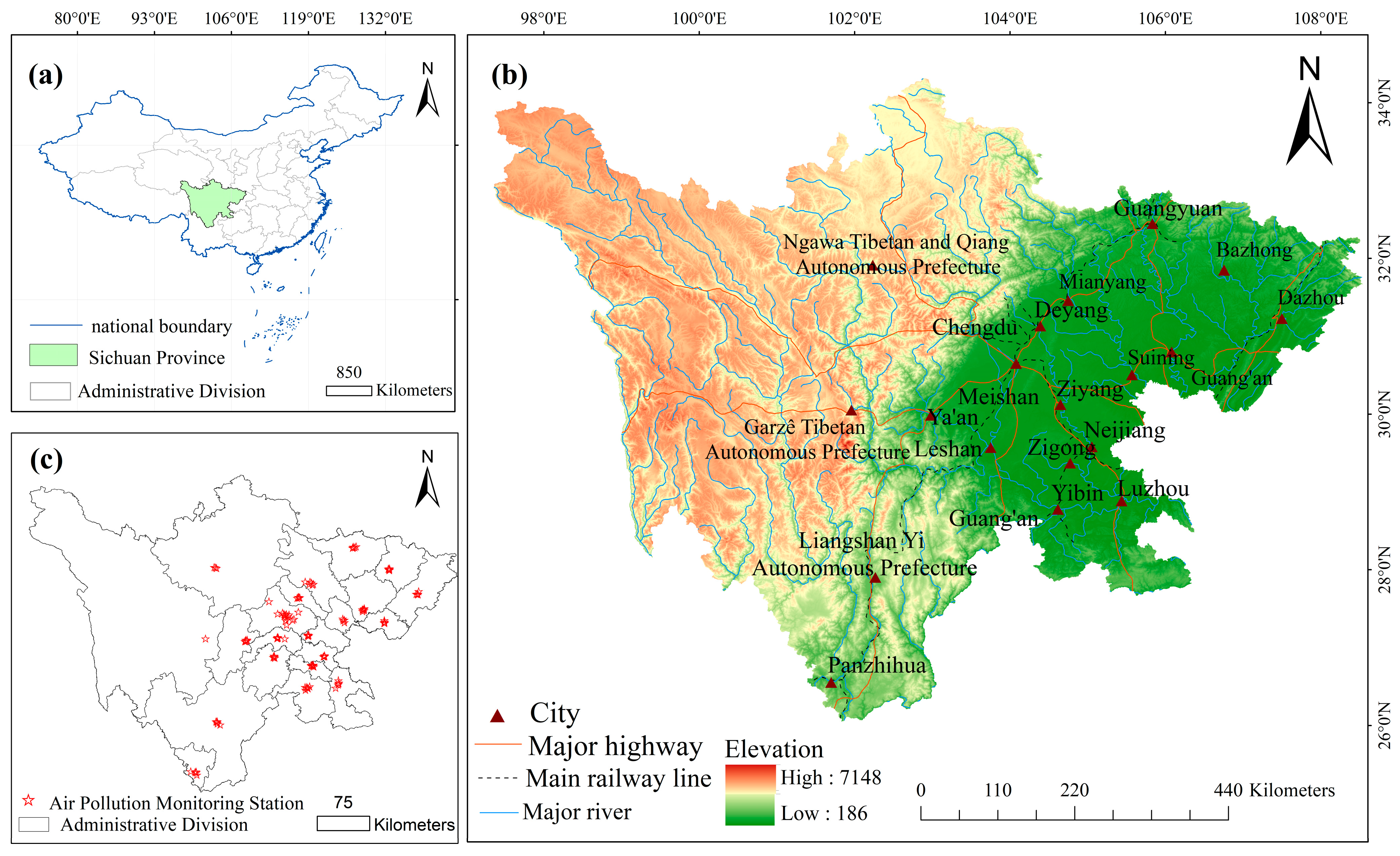
Figure 1. Study Area: (a) the geographical location of Sichuan Province within China; (b) distribution of major cities and topographic map of Sichuan Province; (c) distribution of air pollution monitoring stations across the province.
Atmosphere 16 00958 g001
Figure 2. Technical framework. Note: O3 refers to the maximum daily 8 h average concentration (MDA8).
Atmosphere 16 00958 g002
Figure 3. Structure of the BO–CNN–LSTM–Transformer model.
Atmosphere 16 00958 g003
Figure 4. Dual-channel LSTM structure.
Atmosphere 16 00958 g004
Figure 5. CNN-based feature extraction module.
Atmosphere 16 00958 g005
Figure 6. Transformer prediction module.
Atmosphere 16 00958 g006
Figure 7. Bayesian optimization workflow for LSTM.
Atmosphere 16 00958 g007
Figure 8. Daily average changes of six major atmospheric pollutants from 2021 to 2023. Note: All values are province-level averages across 21 prefecture-level cities. Units: μg/m3 for PM2.5, PM10, SO2, NO2, and O3; mg/m3 for CO.
Atmosphere 16 00958 g008
Figure 9. Spatial distribution of six major air pollutants in Sichuan Province from 2021 to 2023.
Atmosphere 16 00958 g009
Figure 10. Correlation matrix of major air pollutants in Sichuan Province. Note: correlation coefficients are computed using province-level average concentrations from 21 cities.
Atmosphere 16 00958 g010
Figure 11. Comparison of predicted and observed PM2.5 concentrations across different models in Chengdu (January–June 2024).
Atmosphere 16 00958 g011
Figure 12. Residual distribution of PM2.5 predictions in Chengdu across models (January–June 2024).
Atmosphere 16 00958 g012
Figure 13. MAE comparison for six pollutants in Chengdu across forecast models (January–June 2024).
Atmosphere 16 00958 g013
Figure 14. RMSE comparison for six pollutants in Chengdu across forecast models (January–June 2024).
Atmosphere 16 00958 g014
Figure 15. R2 comparison for six pollutants in Chengdu across forecast models (January–June 2024).
Atmosphere 16 00958 g015
Figure 16. Comparison of fitting performance of models on PM2.5 prediction trends in four representative cities. Note: panels a–d represent the four representative cities, respectively: (a) Mianyang, (b) Nanchong, (c) Yibin, (d) Zigong.
Atmosphere 16 00958 g016
Figure 17. Comparison of residual boxplots of PM2.5 prediction among models in four representative cities.
Atmosphere 16 00958 g017
Table 1. Comparison of representative air pollution prediction models.
ModelSpatial FeatureTemporal FeatureGlobal ModelHyperparameter Optimization
MLR [11]/ARIMA [12]
SVM [14]/MLP [15]/RF [16]
LSTM [18]
CNN [19]
FD–BiLSTM [26]
CNN–LSTM [24]
BO–GRU [27]
ARIMA–WOA–LSTM [29]
VMD–Transformer [25]
BO–CNN–BiLSTM–Transformer
(This Study)

(Local Moran’s I)

(BiLSTM + Uni-LSTM)
Table 2. Comparison of summary statistics between raw and processed data.
ItemRaw DataCleaned Data
Number of Stations (sites)123104
Total Data Volume (records)924,198794,664
Number of Missing Values (records)27,2690
Missing Rate (%)17.70%0.00%
Outlier Proportion (3σ, %)0.27%<After 3σ rule interpolation
Outlier Proportion (IQR, %)1.09%<After IQR-based interpolation
Table 3. Year-on-year changes in the annual average concentrations of six pollutants across 21 cities in Sichuan Province (2021–2023).
PollutantsUnit202120222023
AverageAverageChange from 2021AverageChange from 2021Change from 2022
COmg/m30.650.64−1.22%0.61−6.15%−4.01%
SO2µg/m37.657.48−2.18%6.95−9.15%−7.10%
NO2µg/m324.5522.99−6.36%22.62−7.86%−1.61%
O3µg/m312714010.24%1367.09%−2.86%
PM2.5µg/m333.1432.20−2.84%33.982.53%5.54%
PM10µg/m351.5449.82−3.33%53.133.08%6.65%
Table 4. Parameter settings for comparative experiments.
ParametersNumber
Input nodes7
Output node1
Activation functionReLU
OptimizerAdam
Iterations100
Time step size7(9)
batch32
Loss functionMAE
Table 5. Comparison of prediction accuracy between baseline models and ablation experiments.
ModelMetricsPollutants
COPM10PM2.5NO2SO2O3
BO–LSTM [47]MAE15.9013.1010.4013.6914.1114.00
RMSE23.4016.1415.9517.5321.1421.74
R20.600.690.7920.7490.6410.649
WOA–LSTM [48]MAE15.2516.9814.1012.9015.5114.63
RMSE21.1924.4118.9816.9022.7520.06
R20.6130.5160.6520.7090.6080.619
CNN–LSTM [24]MAE11.1311.2311.1611.5210.7310.22
RMSE12.7212.8312.7513.0412.7912.59
R20.7740.7710.7730.7650.7770.782
BO–CNN–LSTM [49],MAE11.0211.2010.758.809.109.50
RMSE13.3013.5012.9012.2012.9012.30
R20.7910.7840.8030.8510.8320.841
WOA–CNN–LSTM [23]MAE8.9011.2010.408.308.518.20
RMSE12.2414.1013.2011.8011.3010.80
R20.8030.7520.7840.8420.8410.851
CNN–LSTM–TransformerMAE9.678.638.548.138.288.80
RMSE13.2511.4612.4310.7810.849.54
R20.8310.8620.8440.8750.8740.872
BO–LSTM–TransformerMAE9.59 8.939.27 10.15 7.32 10.96
RMSE12.47 12.1212.94 13.42 10.7614.89
R20.8040.8340.8150.8070.8630.798
BO–CNN–LSTM–Transformer without LMIMAE10.097.19 8.23 8.47 8.17 7.74
RMSE11.229.5713.99 10.03 9.9710.88
R20.8290.8710.8530.8630.8650.842
BO–CNN–LSTM–TransformerMAE7.386.156.986.677.157.33
RMSE9.898.479.529.5710.299.45
R20.8780.8840.8730.8940.8740.883
Table 6. Distribution of air pollution exceedance days by pollutant type in Chengdu.
CitiesYearPM2.5PM10NO2O3SO2CO
Chengdu202167328000
Chengdu20226173200
Chengdu202352222200
Table 7. PM2.5 exceedance days in four representative cities during 2021–2023.
PollutionYearChengduZigongYibinMianyangNanchong
PM2.5202167545122 28
20226138431418
2023525645 36 35
Table 8. Performance comparison of models in PM2.5 prediction across four representative cities.
ModelMetricsCity
ZigongYibinMianyangNanchong
BO–LSTMMAE13.4 12.84 12.54 11.25
RMSE15.5914.96 16.20 16.74
R20.7530.7580.7340.721
WOA–LSTMMAE13.10 12.2012.03 13.53
RMSE19.3718.6117.68 17.12
R20.6470.6950.7060.643
CNN–LSTMMAE11.9211.79 12.42 12.20
RMSE15.8013.41 14.5715.87
R20.7350.7640.7690.728
BO–CNN–LSTMMAE10.21 10.50 10.5110.54
RMSE14.6212.83 12.6212.46
R20.7940.8160.7930.799
WOA–CNN–LSTMMAE11.46 11.17 10.41 10.66
RMSE16.7515.7112.3213.02
R20.7520.7710.7950.764
CNN–LSTM–TransformerMAE10.95 10.90 9.64 9.30
RMSE13.6612.3011.29 11.86
R20.8170.8430.8010.814
BO–CNN–LSTM–TransformerMAE6.927.34 7.56 7.74
RMSE9.67 9.019.319.55
R20.8710.8830.8840.856
Disclaimer/Publisher’s Note: The statements, opinions and data contained in all publications are solely those of the individual author(s) and contributor(s) and not of MDPI and/or the editor(s). MDPI and/or the editor(s) disclaim responsibility for any injury to people or property resulting from any ideas, methods, instructions or products referred to in the content.