Article

On the Assessment of Hourly Means of Solar Irradiance at Ground Level in Clear-Sky Conditions by the ERA5, JRA-3Q, and MERRA-2 Reanalyses

by
Yves-Marie Saint-Drenan
* and
Lucien Wald
MINES Paris, PSL University, Centre Observation Impacts Energie (O.I.E.), 06904 Sophia-Antipolis, France
*
Author to whom correspondence should be addressed.
Atmosphere 2025, 16(8), 949; https://doi.org/10.3390/atmos16080949
Submission received: 24 June 2025 / Revised: 11 July 2025 / Accepted: 14 July 2025 / Published: 7 August 2025
(This article belongs to the Section Atmospheric Techniques, Instruments, and Modeling)

Abstract

Meteorological reanalyses are one of the means to assess the solar irradiance reaching the ground. This paper deals with estimates of the hourly means of irradiance in clear-sky conditions provided by the ERA5, JRA-3Q, and MERRA-2 reanalyses. They are compared to coincident ground-based measurements from 28 BSRN stations located worldwide, selected by a new algorithm for detecting cloud-free instants. Although ERA5 most often underestimates measurements, it is quite reliable over time because it captures the temporal variability of measurements well and provides a constant level of uncertainty. JRA-3Q offers a complex pattern with negative and positive biases depending on station and season. It captures well the temporal variability but, as a whole, is not reliable over time. None of the three reanalyses is reliable in space. Because of its use of the mean solar time instead of the true solar time, MERRA-2 suffers many drawbacks over intraday scales. Its statistical indicators exhibit marked patterns depending on the season and station. Its assimilation of aerosol properties offers advantages when compared to the climatologies used in ERA5 and JRA-3Q. This work exposes the strengths and weaknesses of each reanalysis in clear-sky conditions and formulates suggestions to providers for further improvements.

1. Introduction

The power of the electromagnetic radiation from the sun that reaches the surface of the Earth is the main driver behind the weather and climate systems on the planet. The density of power received from the sun on a horizontal surface at ground level per unit surface is called the solar irradiance at the surface (SIS) and is expressed in W m−2. It is hereafter abbreviated as SIS and noted E. Equivalent terms may be found in the literature, such as solar flux, surface solar irradiance, downwelling solar irradiance, downwelling shortwave flux, downwelling surface shortwave flux, surface incoming solar radiation, surface incoming shortwave radiation, surface net downward shortwave flux, or global horizontal irradiance. The SIS is usually integrated over the solar spectrum (total SIS).
The Global Climate Observing System (GCOS) program has identified the SIS as an essential climate variable that helps us understand climate evolution and guides adaptation and mitigation efforts [1,2]. The SIS is also one of the essential variables in air quality [3], the terrestrial and marine environment [4,5], and renewable energies [6]. In addition to these domains, it impacts on human health [7] and many other aspects of our daily lives and our activities (see many examples in [8] or [9] (pp. xxii–xxviii)). As a result, there is a significant and rising demand for precise and trustworthy estimates and measurements of the SIS, anytime, anywhere.
Numerical weather prediction (NWP) models, whether used for forecasting or reanalysis, are one of the methods used to estimate SIS. They can offer a global coverage and span of several years. This study focuses on three widely used atmospheric reanalysis datasets: the ECMWF Reanalysis version 5 (ERA5) produced by the European Centre for Medium-Range Weather Forecasts (ECMWF), the Modern-Era Retrospective analysis for Research and Applications version 2 (MERRA-2) developed by NASA’s Global Modeling and Assimilation Office (GMAO), and the Japanese 55-year Reanalysis with Quarterly updates (JRA-3Q) provided by the Japan Meteorological Agency (JMA). Reanalyses derive from weather forecast models used in a reanalysis mode to replicate observed conditions. A wide range of observations—including weather station measurements, satellite data, and GPS signals—are assimilated to estimate atmospheric state variables such as temperature, humidity, and wind speed. A description of the data assimilated in the three reanalysis is given in [10,11,12,13]. In contrast, measurements of the SIS are not assimilated in the three considered reanalyses and the SIS is a diagnostic quantity, derived from all related variables and calculated using a radiative transfer model. It depends on the complete set of radiatively active variables in the atmospheric column above the specific location. Therefore, reanalysis estimates of the SIS should not be confused with direct measurements as they carry the uncertainty inherent in the model simulations such as limited resolution of the model, uncertainties in the parameterizations used, and individual uncertainty of observations.
The SIS E is often written as the product of the SIS received in cloud-free conditions, noted as E c l e a r , and a cloud modification factor, also known as the clear-sky index, noted as Kc.
E = E c l e a r   K c .
A clear-sky index close to 1 would imply a sky without clouds, and a value close to 0 would imply a sky covered by optically thick clouds. Over short time periods, especially in broken-cloud conditions, K c might be greater than 1, resulting from a so-called cloud enhancement effect. Situations may also arise in which K c exceeds 1 over extended periods, notably due to the combination of high surface reflectivity and low solar elevation.
Oumbe et al. [14] showed that at first approximation, K c does not depend on the properties of the cloud-free atmosphere and depends only on the cloud properties and the reflective properties of the ground. This approximation yields errors comparable to the typical uncertainties of pyranometers, except when the ground albedo exceeds 0.7. This result shows that the effects of the cloudless atmosphere are entirely conveyed in the modelling of E c l e a r and highlights the importance of accurate assessment of E c l e a r . Clear-sky models aim at estimating E c l e a r . They provide realistic upper limits of the SIS and contribute indirectly to quantifying the radiative effects of clouds. E c l e a r varies with the date, time of day, geographic location, and gas concentrations. For total SIS, aerosol, water vapor, and ozone are the most influent variables, while other gases can be assigned standard concentrations. Extinction also depends on local temperature, density, pressure, and volume mixing ratio for the non-ozone, non-water vapor gases, necessitating knowledge of the vertical profiles of these variables, which is crucial for calculating the scattering effects from air molecules. Additionally, E c l e a r is influenced by the elevation and reflective properties of the ground.
The present paper builds upon the result from [14] and focuses on the estimates of the hourly means of E c l e a r E c l e a r h , made by each of the three reanalyses considered in the present work. More precisely, it aims at assessing the quality of these estimates by a comparison against coincident high-quality ground-based measurements of E c l e a r h . It is an attempt to identify potential drawbacks in the modelling of E c l e a r h and may help the agencies in charge of the reanalyses in further developments as uncertainties in E c l e a r h affect the estimates of the SIS in all conditions.
There are many scientific articles relating to the comparison between estimates of E from reanalyses and ground-based measurements on hourly, daily, monthly, or yearly basis. To the best of our knowledge, based on a comprehensive survey of the literature, none of them was dedicated to clear-sky conditions, except [15], and none of them explored the clear-sky products of these reanalyses except [15,16].
Wang et al. [15] compared the monthly mean of the clear-sky product of MERRA-2 E c l e a r _ m e r r a 2 m o n t h to ground-based measurements of E c l e a r m o n t h under cloudless skies in Asia obtained by thresholding the monthly clearness index K T m o n t h , where the clearness index is the ratio of E to the corresponding extraterrestrial irradiance received on a horizontal surface located at the top of the atmosphere, noted as E 0 . They found that MERRA-2 overestimates E c l e a r m o n t h and K T c l e a r m o n t h significantly. Working with hourly measurements in the tropical Atlantic Ocean, Trolliet et al. [16] did the sole study comparing the hourly clear-sky product from MERRA-2, E c l e a r _ m e r r a 2 h , and the corresponding SIS E M c C l e a r h from the McClear service of the Copernicus Atmosphere Monitoring Service (CAMS) [17,18], whose quality is well documented [19]. Without providing any number, they reported that these datasets are similar and concluded that the MERRA-2 cloud-free SIS are likely accurate. As clear-sky products of ERA5 were unavailable at that time, the authors performed a visual inspection of daily profiles of E e r a 5 h for randomly selected cloud-free days on which daily profiles of E M c C l e a r h were superimposed and found that E M c C l e a r h was underestimated by ERA5 in these cases.
In addition to [15,16], several studies have partially investigated clear-sky conditions. They dealt with ground-based measurements in several places: Scandinavia [20], South Africa [21], West Africa [22], Pakistan [23,24], Indonesia [25], or worldwide [26]. Clear-sky conditions were determined using various approaches. Some works select clear sky instants by thresholding the daily clearness index K T d a y [22,23,25,26], or modified clearness index [24], and others use the daily clear-sky index when an external clear-sky model is used [20]. Mabasa et al. [21] did not detail how the clear-sky days were determined, but from [19], it appears that they used ERA5 in a first step and then a combination of a modified version of the algorithm of Reno and Hansen [27] and McClear outputs.
This survey of the literature reveals several discrepancies in results. Several of them may be partly explained by discrepancies in the studied timescale, from hour to month. For example, Wang et al. [15] report that MERRA-2 overestimates E c l e a r m o n t h and K T c l e a r m o n t h significantly while others [23,24,25,26] wrote that MERRA-2 slightly underestimates the daily means E c l e a r d a y , and Trolliet et al. [16] concluded that MERRA-2 cloud-free hourly means, E c l e a r _ m e r r a 2 h , are likely accurate. Other partial explanations of the discrepancies may be due to differences in the studied areas and periods as the quality of the estimates of the cloudless SIS may depend on the climate and changes in aerosol properties and water vapor among others. Discrepancies are also partly due in the manner of determining clear-sky conditions, as discussed above, as it has a great influence on results [19,28].
From this survey of the literature, we observed several discrepancies in results that may be partly explained by discrepancies in the studied timescale, discrepancies in the geographical area, and by discrepancies in determining clear-sky conditions, the latter having a great influence on results [19,28].
Sianturi et al. [25] reported that ERA5 estimates E c l e a r d a y fairly correctly, in contradiction with other studies [23,26] that found a slight underestimation of E c l e a r d a y , or an overestimation [20]. ERA5 was found to report cloudy conditions while the actual conditions are cloud-free [16,21,26], and in another study ground-based measurements and ERA5 agree on the clear-sky category 77% of the time [20]. As for JRA-55, the predecessor of JRA-3Q, the sole study reported that JRA-55 tends to underestimate E c l e a r d a y [23]. As for MERRA-2, it slightly underestimates E c l e a r d a y [24,25,26] but Wang et al. found that it overestimates E c l e a r m o n t h significantly.
These works give some indications of the ability of ERA5, JRA-3Q, and MERRA-2 to reproduce E c l e a r on hourly, daily, and monthly bases though they provide little quantitative measurement of it, except for [15]. Our study focuses on hourly means of the clear-sky SIS E c l e a r h and aims at extending the current knowledge as we believe that it would be fruitful to better know the strengths and weaknesses of the reanalyses in clear-sky conditions for further improvements in the diagnostic of E in all conditions. The present paper does not intend to rank reanalyses. There are many reasons for choosing one reanalysis over others; a ranking based solely on comparisons with in situ measurements at a limited number of stations during a limited period is unlikely to cover all needs and constraints.
Figure 1 exhibits an overview of the methodology adopted for this paper, with details given later for each step. The ground-based measurements collected every 1 min in the BSRN network [29], noted as E b s r n m i n , are checked for their plausibility. Detection of clear-sky instants is made on the retained 1 min data, yielding the time series E c l e a r _ b s r n m i n . From this series, hourly means of SIS in cloudless conditions, noted as E r e f h , are created and are compared to the coincident estimates of E c l e a r h given by each reanalysis. The comparisons are also performed on the clearness index K T r e f h . As the estimates of the SIS depend on the calculation of the extraterrestrial irradiance E 0 h made by each reanalysis, a comparison is performed between the various E 0 h to check their consistency. This is justified in the case of MERRA-2 as it was reported in [16] that MERRA-2 is using the mean solar time and does not account for the difference between the true solar time and the mean solar time, which is a function of the day in the year as a first approximation, thus bringing additional uncertainty in the estimates of E h .
The data and models are briefly presented in Section 2. The protocol for validation is described in Section 3. The verification of the extraterrestrial irradiance E 0 h is discussed in Section 4. There are several ways of discussing results when several models are dealt with. Here, the selected approach is to present and discuss the results of each reanalysis separately in Section 5, Section 6, and Section 7, respectively, so that each Section provides the reader with a full view of the performances of a given reanalysis. Section 8 concludes the paper. How to access the data is described in the “Data availability” section.

2. Data and Models

Data used here are measurements of E b s r n m i n performed in the BSRN network, estimates of E c l e a r h from the reanalyses ERA5, JRA-3Q, and MERRA-2, as well as estimates of several cloudless atmosphere properties derived from CAMS.

2.1. Selected Sites and Periods

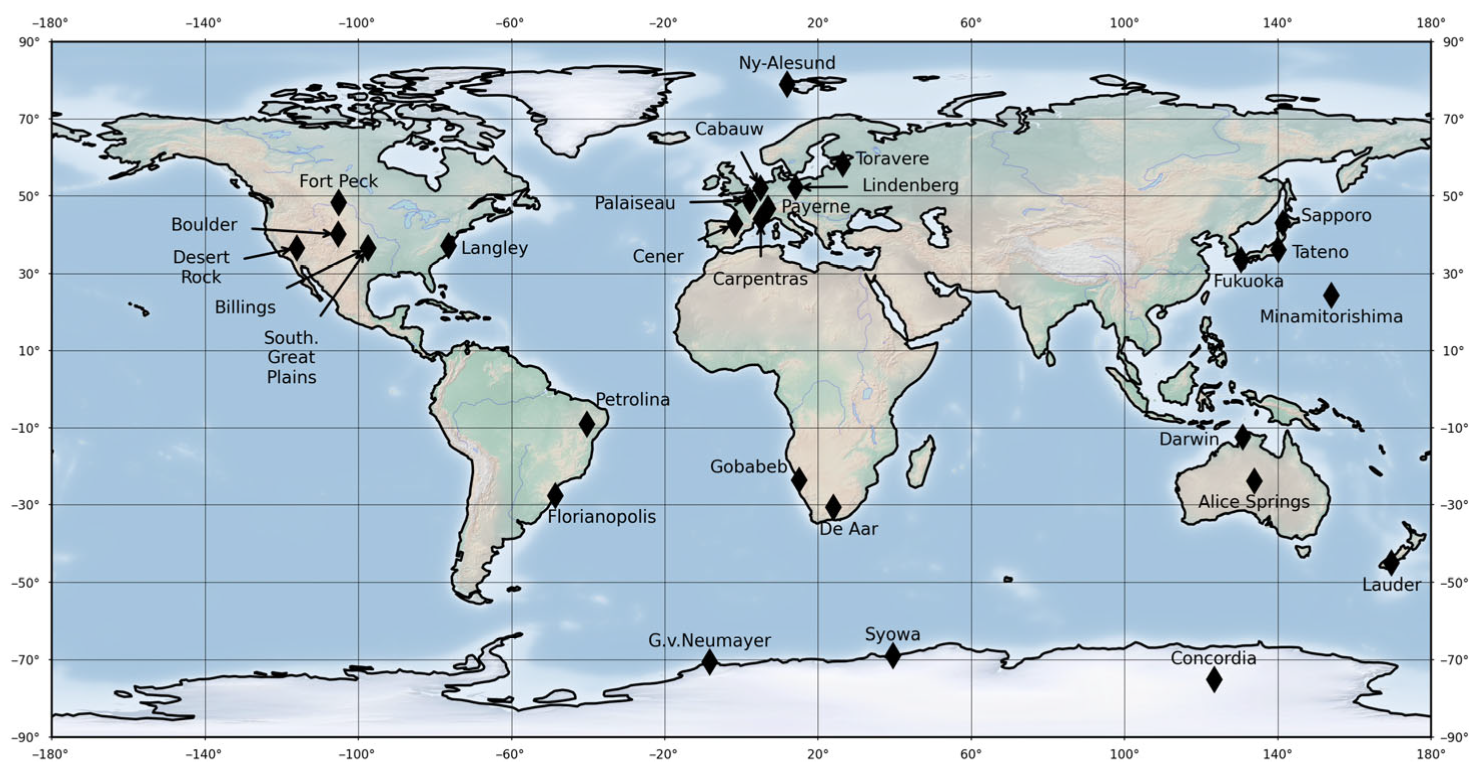
Ground-based measurements were obtained at 28 sites located worldwide belonging to the Baseline Surface Radiation Network (BSRN) [29] (Figure 2 and Table 1). These stations exist in a variety of climates. In order to perform trimester-based comparisons consistent with climatological convention (DJF, MAM, JJA, and SON), each year is defined as beginning in the preceding December. For instance, DJF 2017 covers the period from December 2016 to February 2017. With this convention, the selected periods are [2015-12-01 to 2016-11-30], [2016-12-01 to 2017-11-30], and [2017-12-01 to 2018-11-30]. For the sake of conciseness, they are designated as 2016, 2017, and 2018. These three years were chosen as they represent the most recent periods with the greatest number of BSRN stations providing high data availability.

2.2. Reanalyses

This study deals with ERA5 developed at the ECMWF (European Centre for Medium-Range Weather Forecasts) [10], JRA-3Q (Japanese Reanalysis for Three Quarters of a Century) of the Japan Meteorological Agency [12], a follow-on of the JRA-55 reanalysis [11], and MERRA-2 (Modern-Era Retrospective Analysis for Research and Applications, version 2) of the USA National Aeronautics and Space Administration [13]. The sizes of the grid cell of the solar radiation variables are 0.28125° × 0.28125° (31 km in latitude) for ERA5, 0.375° × 0.375° (42 km in latitude) for JRA-3Q, and 0.5° in latitude (56 km) by 0.625° in longitude (70 km at the Equator) for MERRA-2.
Of particular importance for the modelling of the downwelling solar radiation in clear-sky conditions at surface is the modelling of the aerosol properties. ERA5 exploits a prescribed monthly climatology from Tegen et al. [30] for tropospheric aerosols and Tanre et al.’s [31] aerosol climatology as well as GISS dataset [32] for stratospheric aerosols [10]. Similarly, JRA-3Q, like JRA-55, relies on a fixed aerosol climatology derived from the MODTRAN/GINA model [11]. In contrast, MERRA-2 includes a system based on the GOCART model, with assimilation of satellite-derived aerosol optical depth (e.g., MODIS and AVHRR), and a direct coupling to radiative transfer [13,33].
The solar radiation at the top of the atmosphere and downwelling solar radiation in clear-sky conditions at surface were downloaded from the ECMWF Copernicus Climate Datastore (CDS) for ERA5, Thredds data server operated by UCAR for JRA-3Q, and NASA Earthdata website for MERRA-2 at the four nearest grid cells to each site. All time series are in UT time system. A spatial bilinear interpolation technique with a weighting factor that is inversely proportional to the distance to the site was then applied to yield time series of hourly means of irradiance at the site, noted, respectively, as E 0 _ e r a 5 h , E c l e a r _ e r a 5 h , E 0 _ j r a 3 q h , E c l e a r _ j r a 3 q h , E 0 _ m e r r a 2 h , and E c l e a r _ m e r r a 2 h . Then time series of clearness index are derived as follows:
K T c l e a r _ e r a 5 h = E c l e a r _ e r a 5 h E 0 _ e r a 5 h ,
K T c l e a r _ j r a 3 q h = E c l e a r _ j r a 3 q h E 0 _ j r a 3 q h   ,
K T c l e a r _ m e r r a 2 h = E c l e a r _ m e r r a 2 h E 0 _ m e r r a 2 h .

2.3. Astronomical Quantities and Others

Several astronomical quantities were extracted from CAMS in UT time to help analyse the results of the comparisons. For convenience, we used the McClear service in CAMS, which in its verbose mode delivers among other quantities 1 min values of readings from CAMS resampled to the selected location by spatial bilinear interpolation and resampled in time by linear interpolation, namely the solar zenithal angle θ S m i n calculated with the SG2 algorithm [34], and the irradiance at the top of the atmosphere E 0 m i n using the nominal total solar irradiance of 1361 W m−2, as recommended by [35]. A second call to the McClear service, this time for hourly values, returned the irradiance at the top of the atmosphere, E 0 h , as well as the hourly direct components of the clear-sky model McClear on a horizontal surface, B M c C l e a r h , and on a plane always normal to the sun’s rays, B N _ M c C l e a r h . The last two quantities were used to calculate an effective solar zenithal angle θ S e f f _ h for each hour [36]:
θ S e f f _ h =   cos 1 ( B M c C l e a r h B N _ M c C l e a r h ) .
Because of the high accuracy of the SG2 algorithm, the irradiance E 0 h is considered as a reference to which E 0 _ e r a 5 h , E 0 _ j r a 3 q h , and E 0 _ m e r r a 2 h are compared.

2.4. BSRN Measurements and Their Filtering

Stations in the BSRN network perform high-quality measurements of the SIS and its diffuse and direct components [29]. Each station is equipped with class-A thermopile pyranometers, one of them being equipped with a shadow ball mounted on a tracker, to separately measure E b s r n m i n and D b s r n m i n , and a pyrheliometer to measure the direct component at normal incidence, B N _ b s r n m i n . The measurements have a temporal resolution of 1 min. Uncertainty requirements are 5 W m−2 for E b s r n m i n and D b s r n m i n (2% in relative value) and 2 W m−2 for B N _ b s r n m i n (0.5%) [29].
The BSRN-recommended quality check [37] was applied to the measurements and only those flagged as non-suspicious were retained here. For the sake of clarity in writing, the retained measurements are said to be “valid”. For further use, the clearness index is computed as follows:
K T b s r n m i n = E b s r n m i n E 0 m i n .

2.5. Screening of Cloudless Instants

A new algorithm for detecting cloud-free instants has been devised taking into account the comments of Bright et al. [28] on the existing ones. Its principle is that the 1 min SIS in clear-sky conditions exhibit smooth variations, or, said differently, its derivative is continuous. It is also the case for the SIS in overcast conditions, and such cases must be excluded. As it is usually impossible to compute derivative from fragmented series of measurements, the problem is reversed to keep only measurements that are close to an analytical function that fits typical SIS in clear-sky conditions. The proposed algorithm is meant to reliably detect cloud-free instants and not all cloud-free instants. Hence, it may reject actual cloud-free measurements.
The algorithm comprises several cascading dyadic multi-scale filters that apply to the valid 1 min measurements for each day of the time series. It exploits the form of the MLB function [38] for interpolating the SSI as a function of the solar zenithal angle θ S m i n in clear-sky conditions:
E M L B m i n =   E 0 m i n e x p b c o s ( θ S m i n ) a ,
where the parameters a and b are adjusted by a least-squares technique on all valid E b s r n m i n within a sliding window of width ± n/2 min, centred on each instant t, expressed in min, in the day. Each interval [t − n/2, t] and [t, t + n/2] must contain at least 30% of valid values, B N b s r n m i n , greater than 10 W m−2. Otherwise, the instant t is said to be “likely cloudy” and the next instant, t, is processed. This constraint is meant to discard homogeneous overcast conditions. If the constraint is met, the MLB function is adjusted, and a series of irradiances noted as E M L B m i n is computed with Equation (7).
Over each window of length 2*n, the covariance C o v n m i n between E M L B m i n and valid E b s r n m i n and the variances V a r b s r n , n m i n and V a r M L B , n m i n of the valid E b s r n m i n and coincident E M L B m i n are computed for each time step, t, in the window [t − n/2, t] and [t, t + n/2]. The instant t is declared as “likely cloud-free” if
C o v n m i n > ρ n m i n × V a r M L B , n m i n × V a r b s r n , n m i n + σ 2
where ρ n m i n and σ were set empirically to 0.999 and 4 W m−2.
This procedure generates a time series of binary values denoting the results of the clear-sky detector over a temporal window of length 2*n. Four windows were used, with n successively being 120, 60, 30, and 15. Our method finally flags as cloud-free the instants classified as cloud-free over all considered windows. The retained 1 min values are noted as E c l e a r _ b s r n m i n and K T c l e a r _ b s r n m i n .
The algorithm was first verified with ideal cases of clear conditions simulated by the McClear service, then with simulated cases of clear skies including the slow appearance of thin clouds, and, eventually, by visual inspection of randomly selected days in the BSRN dataset. Its outcomes were also compared to those of the algorithms of Lefèvre et al. [17] and Reno and Hansen [27] for a further check of the proper functioning of the algorithm, though the objective of this paper is not to compare the results of our algorithm to others, as in [28].
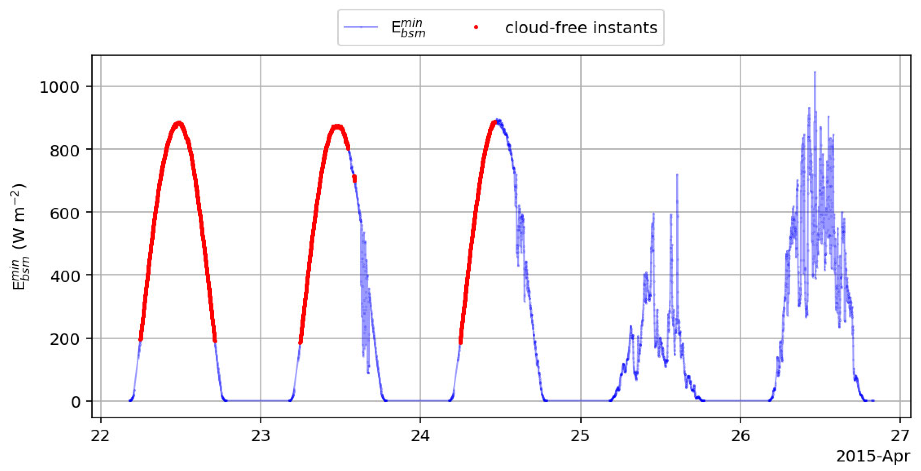
Figure 3 displays several daily profiles of E b s r n m i n at Payerne, on which symbols representing the clear-sky instants detected by our algorithm (red dots) are superimposed. The sequence of five days displayed in Figure 3 includes various sky conditions varying from overcast to cloud-free conditions. As expected, instants with overcast (25 April 2015) and broken clouds (26 April) are rejected by the clear-sky detector. Our algorithm detected clear-sky periods during mixed conditions on 23 and 24 April 2015, while instants with a high variability were excluded. Note that on these two days there was a latency between a period with fluctuating SIS and a detected cloud-free condition. This is intentional to ensure that the selected instants are cloud-free conditions for sure. Finally, on 22 April 2015, the complete day was detected as being cloud-free when the SIS was greater than 200 W m−2. The correct behaviour of our clear-sky detection algorithm was further verified by a visual inspection of other periods and stations.

2.6. Hourly Values

From the time series of E c l e a r   b s r n m i n , hourly means, E r e f h , adjusted onto the time-stamping in UT used by the three reanalyses were constructed by a linear interpolation in K T c l e a r   b s r n m i n for filling in the gaps, provided there are at least 20 known K T c l e a r _ b s r n m i n in the hour. Otherwise, the hour is said to be invalid. The hourly clearness indices, K T r e f h , were computed as the ratio of E r e f h to E 0 h . These series E r e f h and K T r e f h are the reference against which the estimates of the reanalyses are compared. Their means and variances are termed reference means and variances hereafter.
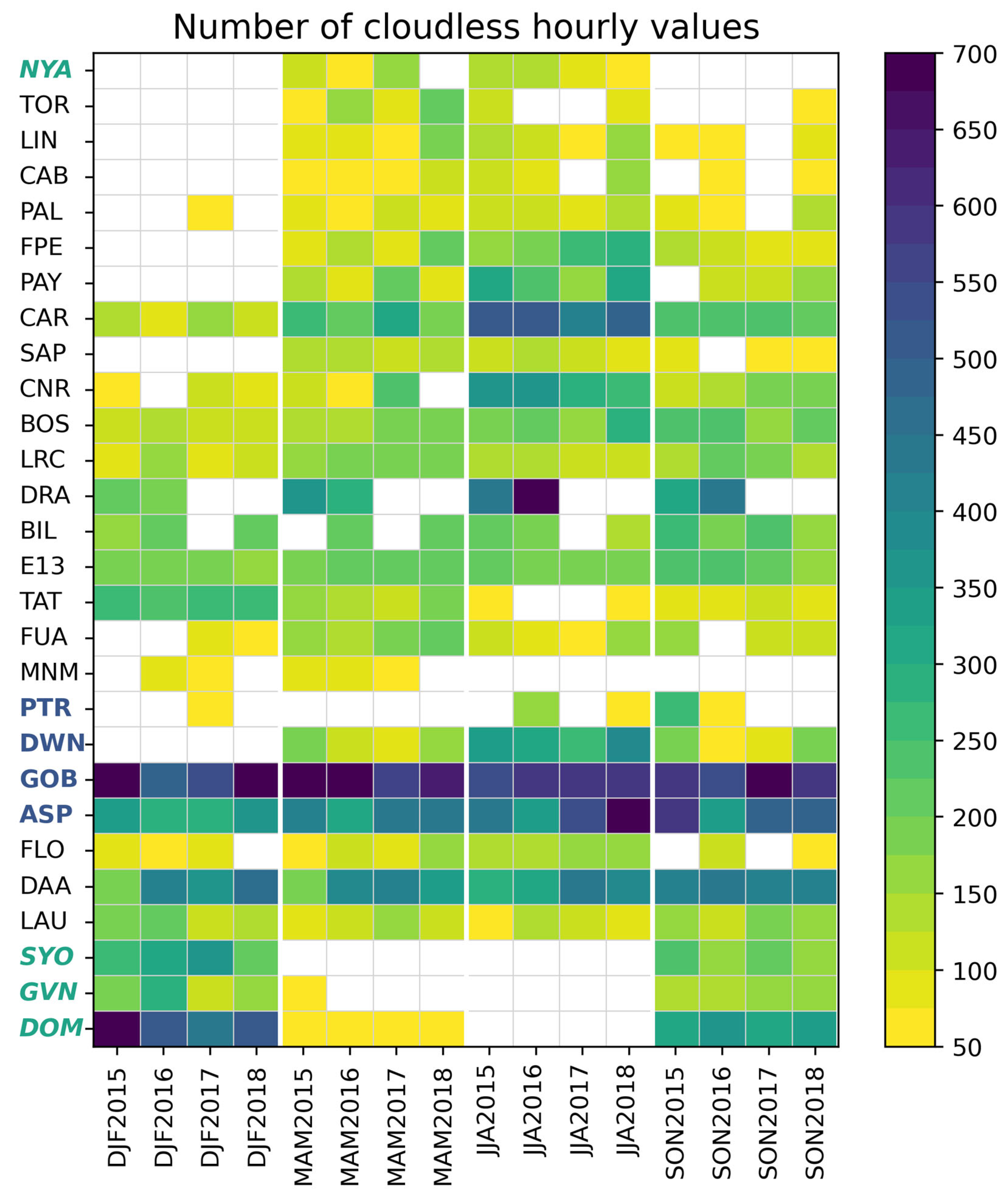
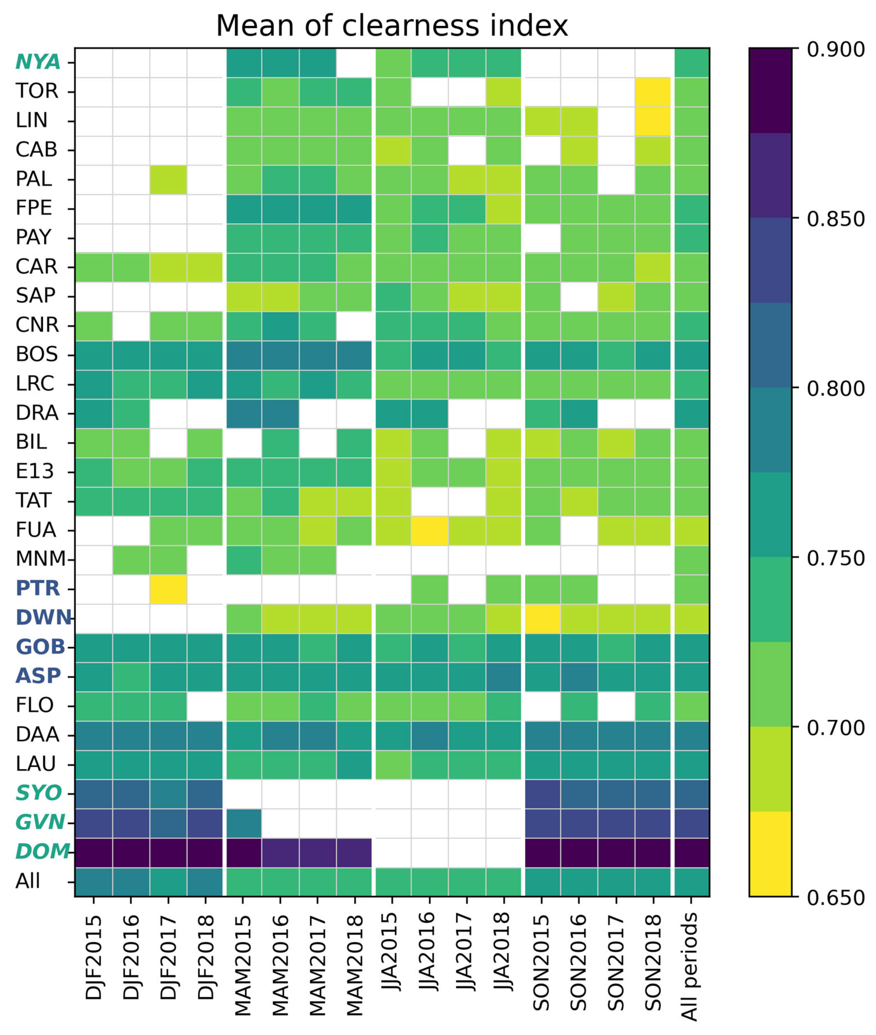
Figure 4 exhibits the number of hours at each station and all stations merged for each period and all periods. Only periods with at least 50 valid hourly values were retained. The number of stations times the number of valid trimesters makes a total of 333 trimesters. Means of E r e f h and K T r e f h at each station and all stations merged are shown in Figure 5 and Figure 6 for each period and all years. The minimum and maximum of E r e f h _ m e a n are 306 W m−2 (DJF207 at Palaiseau (PAL)) and 846 W m−2 (DJF2017 at Florianopolis (FLO)); those of K T r e f h _ m e a n are 0.654 (SON2018 at Toravere) and 0.900 (DJF2015 at Concordia Dome C (DOM)). The greatest K T r e f h _ m e a n are observed at the three Antarctic stations. The snow-covered ground reflects part of the solar irradiance and contributes to the measured SIS, thus increasing the clearness index. In addition, the Concordia Dome C is located at 3233 m above the mean sea level, which means a thinner atmospheric layer and, therefore, a greater clearness index.

3. Protocol for Comparison

There are two kinds of comparison, one deals with the extraterrestrial irradiance, the other with the SIS. The protocol is fairly similar in both cases and applies to each reanalysis in turn. The comparison for the SIS was performed at each BSRN site and for all sites merged, for each trimester and for the ensemble of trimesters.
For each reanalysis, the comparison was made on the estimates provided by this reanalysis and either the extraterrestrial irradiance from the CAMS McClear service E 0 h , or reference values E r e f h and K T r e f h for coincident instants only. The Pearson correlation coefficients, slopes, and offsets of the least-squares fitting lines were computed as well as the differences between coincident estimates and reference values, which were summarized by their mean, known as the bias or mean bias error, their standard deviation, and their root mean square error (RMSE). Relative biases, relative standard deviations, and relative RMSEs were expressed with respect to the reference means. Two-dimensional histograms of reference values and estimates were drawn. In addition, results were analysed as a function of the station, latitude, climate, elevation, year, θ S e f f _ h , reference means, and variances to evidence possible trends. All produced graphs are available as Supplementary Materials.
The present protocol is not new and is similar to many used in comparable studies. It presents several drawbacks that may affect the comparison.
First of all, the reanalyses provide total irradiance, i.e., integrated over the whole spectrum, while BSRN measurements taken by pyranometers are based on a more limited range, as shown in Table 1. The often-used BSRN spectral range [285, 2800] nm accounts for about 99% of the total irradiance with slight dependence on the optical properties of the clear atmosphere constituents and the air mass. The 1% irradiance difference resulting from the limited spectral sensitivity of the pyranometer is partly compensated for during the assessment of the sensitivity coefficient of the instrument, which is the conversion factor between measured thermopile voltage and solar irradiance. The sensitivity coefficient is determined during the calibration of the instrument by comparing readings of the pyranometer and the World Radiometric Reference given by cryogenic solar absolute radiometers that measure total irradiance with a very high accuracy (see [39,40] for details). Consequently, the sensitivity coefficient implicitly accounts for the average difference between the irradiance in the interval [285, 2800] nm and the total irradiance. This suggests that a slight difference, with a zero mean and dependence on air mass and atmospheric content, may exist between the reanalyses and measurements due to the difference in spectral ranges (see [19] for further discussion on the difference in spectral ranges between measurements and models).
A second drawback is due to the mismatch in spatial representation of the field of E by the reanalyses and the BSRN pyranometers. The reanalyses provide E on cells several kilometers in size and, thus, do not contain the sub-cell variability of E that is partly perceived by the pyranometers. This adds to the discrepancy expected between the reanalyses’ outputs and E r e f h , whose magnitude cannot be predicted as it depends on the atmospheric conditions experienced by each station every 1 h. This is a well-known issue that encompasses the present case and applies to many domains in Earth sciences and others. Several examples are provided in [19] showing the large spatial variability of the SIS.
Also to be taken into account is the site elevation as well as the presence of seacoasts or mountains and, more generally, of orographic discontinuities. Urraca et al. [26] reported an increased positive bias in E due to the large size of the grid cells of ERA5 or MERRA-2 over the coasts where the spatial variability in E may be large. This effect may be minimized by a proper choice of BSRN stations located in homogeneous areas with respect to orography, vegetation, or the presence of large water bodies. The limited horizontal and vertical resolutions of the elevation model used in each reanalysis can also bring about a systematic error when the assumed elevation is less than the actual elevation of the station as it may imply, for example, a greater aerosol optical depth or water vapor content.
A final point is the uncertainty affecting the references E r e f h and K T r e f h , which should not be neglected. This uncertainty is a combination of the uncertainty of the measurements themselves and of the construction of the hourly values with gaps.

4. Verification of the Extraterrestrial Irradiance Received on a Horizontal Surface

There is no measurement of the extraterrestrial irradiance at hand. This section aims at verifying the consistency over a year between the extraterrestrial irradiance received on a horizontal surface from the CAMS McClear service, E 0 h , and that from each reanalysis, E 0 _ e r a 5 h , E 0 _ j r a 3 q h , and E 0 _ m e r r a 2 h . Differences ( E 0 _ e r a 5 h E 0 h ), ( E 0 _ j r a 3 q h E 0 h ), and ( E 0 _ m e r r a 2 h E 0 h ) were computed and analyzed. Null values were excluded from the analysis.
The nominal total solar irradiances of the CAMS McClear service and each reanalysis are very close: 1361 W m−2, 1361.6 W m−2, 1365 W m−2, and 1365.2 W m−2, respectively, for McClear service [18], ERA5 [10], JRA-3Q (according to ancillary metadata), and MERRA-2 [41]. This would be reflected in a small bias in the extraterrestrial irradiance. The standard deviation of the differences should be close to 0 and the correlation coefficients should be close to 1, meaning that E 0 h and reanalyses vary similarly in time with similar amplitudes of the variations. As the extraterrestrial irradiance received on a horizontal surface depends on the latitude, the bias and standard deviations of differences depend on latitude too and exhibit symmetry in latitude, i.e., they do not depend on the hemisphere. They are greatest in the tropical belt and tend to decrease as the latitude increases northward or decreases southward. There is very little variation with the year. Table 2 provides results at latitudes 0° and 45° and year 2017 for illustration. Although the actual numbers depend on latitude, conclusions do not.
The values for ERA5 and JRA-3Q are close to expectations. It is concluded that E 0 h , E 0 _ e r a 5 h , and E 0 _ j r a 3 q h are very similar, except for the nominal total solar irradiance. Note that this difference in the nominal total solar irradiance does not affect the computation of the clearness index (Equations (2) and (3)).
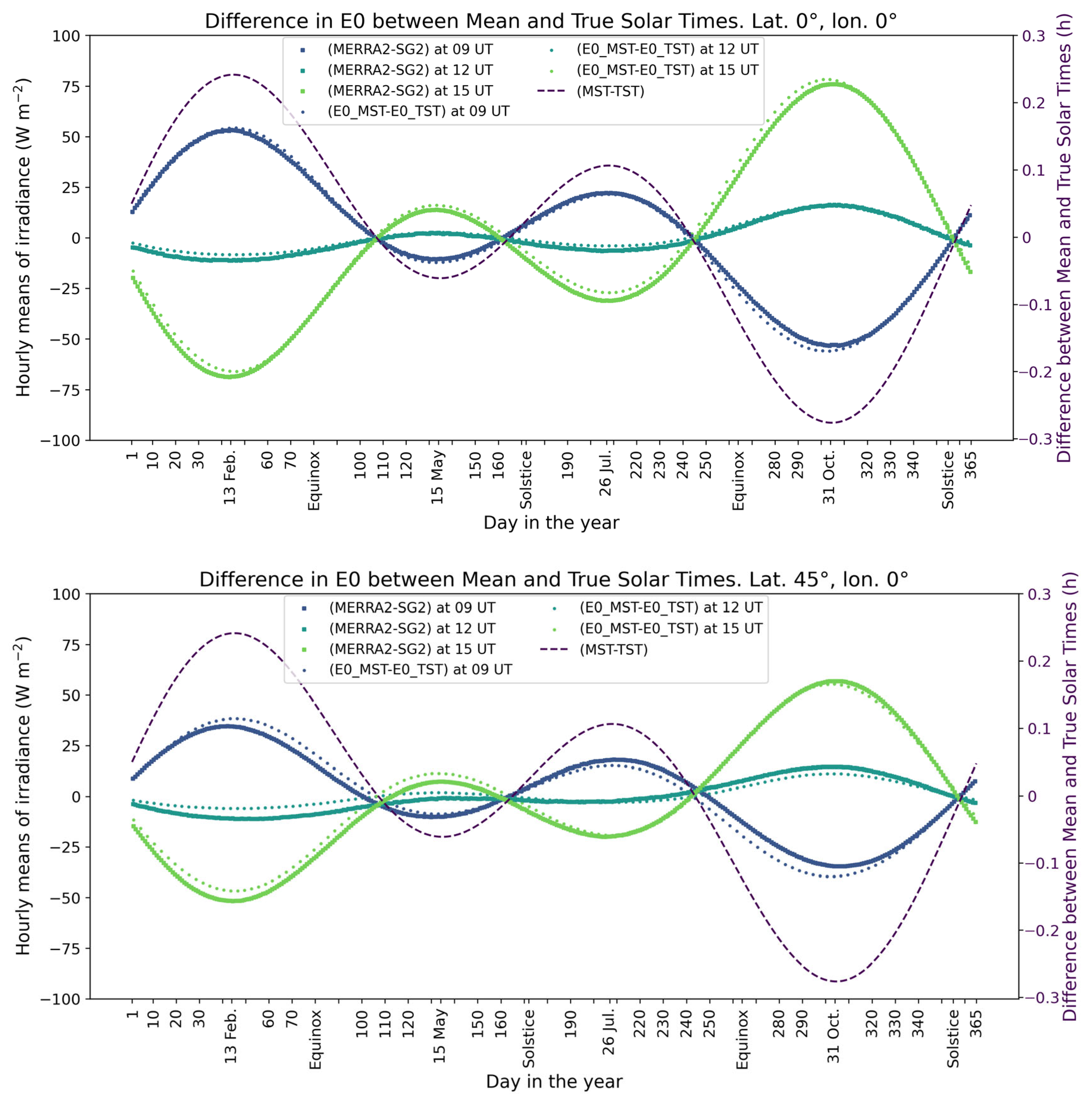
As for MERRA-2, the bias is close to 0 and the correlation coefficient is close to 1, although a little less. However, the standard deviations of the differences are much greater than expected: 34 W m−2 and 21 W m−2 (Table 2), instead of 0 W m−2. To further investigate this discrepancy between E 0 _ m e r r a 2 h and E 0 h , Figure 7 displays the differences ( E 0 _ m e r r a 2 h E 0 h ) at 09:00, 12:00, and 15:00 UT at longitude 0° and two latitudes, 0° (top) and 45° (bottom), across the year. During a given day, the differences ( E 0 _ m e r r a 2 h E 0 h ) can vary from one hour to the next in a non-negligible way. They are close to 0 W m−2 at 12:00 UT and increase in absolute value with θ s for a given day, although they decrease as latitudes increase or decrease towards the poles. They also vary throughout the year for a given hour.
Such variations are not expected and are reminiscent of those between the mean solar time (MST) and the true solar time (TST), which are drawn with the secondary axis in Figure 7, by means of equations taken from [9]. It is visible that ( E 0 _ m e r r a 2 h E 0 h ) vary over the year in correlation or anticorrelation with the difference (MST–TST). The MST is defined in such a way that it is equal to 12:00 on average over the year when the sun reaches its highest during a day. It is equivalent to the UT time at longitude 0°. Due to slight changes in the angular speed of the Earth along its elliptical orbit, the sun does not reach its highest at 12:00 MST every day. The peak time defines the TST, which may differ from 12:00 MST by up to ±15 min approximately. This difference is often termed “equation of time” though it is not an equation in the usual sense. It depends on the eccentricity and obliquity of the orbit. Using the MST instead of the TST has an impact on the calculation of the solar zenithal angle θ S as the latter depends on the TST, and, therefore, it impacts the calculation of the extraterrestrial irradiance, and further the SIS. E 0 h , E 0 _ e r a 5 h , and E 0 _ j r a 3 q h are calculated with the TST and do not exhibit such behavior.
Despite their efforts, the present authors found no explicit mention of MST or TST in the calculation of radiation in MERRA-2 in publicly available documentation. Trolliet et al. [16] have suspected that the MST is used in MERRA-2 instead of the TST for computing θ s and E 0 _ m e r r a 2 h . This hypothesis, already partially confirmed by Figure 7, is studied in more detail in the following. The authors acknowledge that this development is somewhat lengthy but emphasize the need to understand the origin of the error in MERRA-2, which deeply influences the MERRA-2 SIS under clear-sky conditions and, moreover, under all sky conditions at intraday timescales.
The hourly extraterrestrial irradiance in MST E 0 _ M S T h and in TST E 0 _ T S T h were calculated over a year using equations in [9]. These equations are not very accurate but were used here for illustration purposes only. The differences ( E 0 _ M S T h E 0 _ T S T h ) were superimposed onto those ( E 0 _ m e r r a 2 h   E 0 h ) in Figure 7. It is clear that, at a given hour and latitude, the differences are similar. They have the same shape and the same amplitude; their averages differ by −1 W m−2 at both latitudes. The standard deviations of their differences are 2 W m−2 at 0° and 3 W m−2 at 45° and the correlation coefficient is equal to 0.997 and 0.988, respectively. This gives credence to the use of the MST instead of the TST in MERRA-2 and to a miscalculation of the solar zenithal angle, which implies subsequent errors in E 0 _ m e r r a 2 h and SIS E m e r r a 2 h .
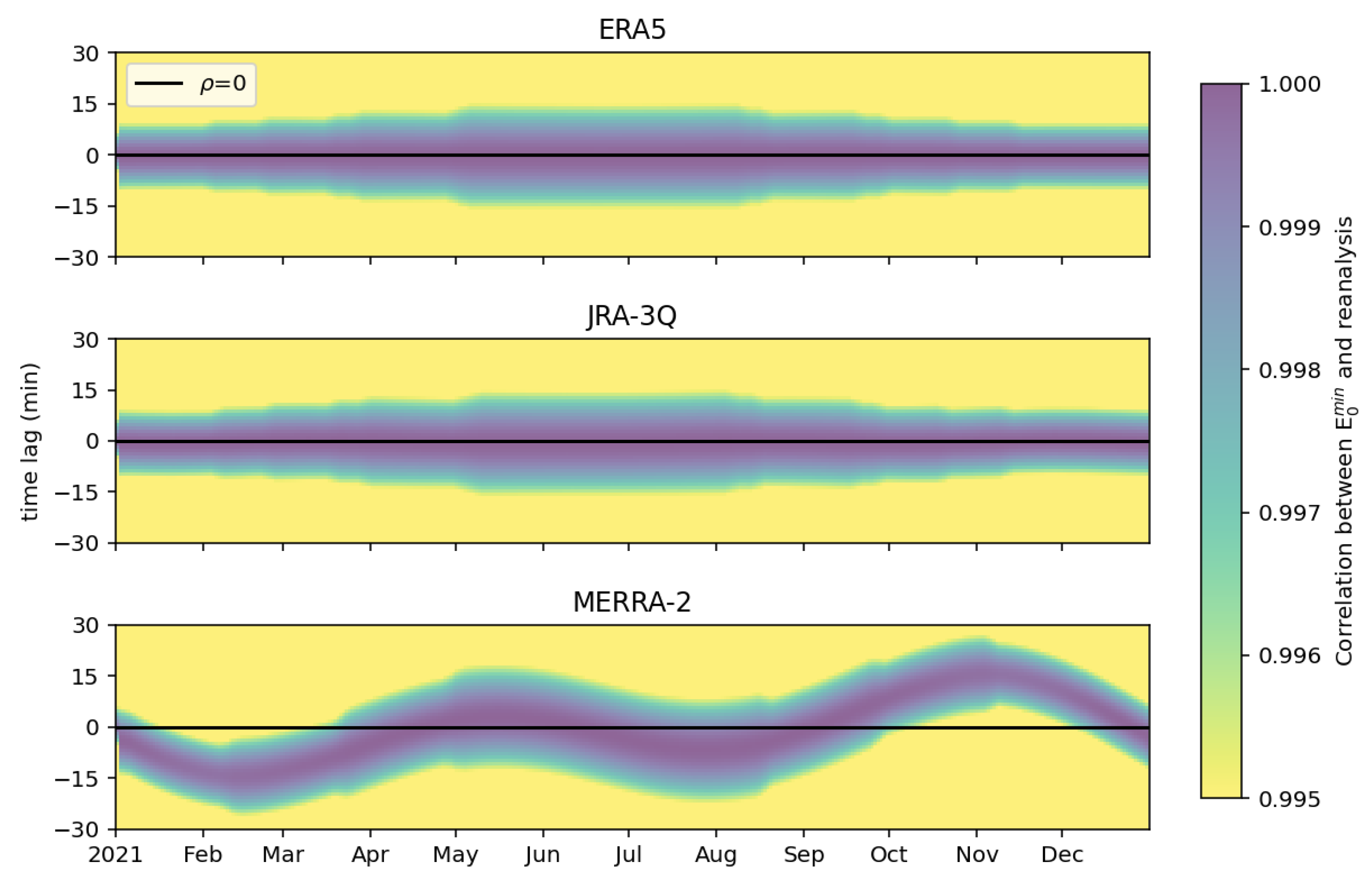
A cross-correlation analysis between E 0 h and E 0 _ e r a 5 h , E 0 _ j r a 3 q h , and E 0 _ m e r r a 2 h , respectively, was conducted to further verify that the lower correlation and higher bias observed for MERRA-2 is related to the omission of the equation of time. Indeed, if the time reference is correct, a maximum correlation will be obtained for a time lag equal to zero and only for this time lag. Otherwise, if the equation of time is omitted, the error in time is diagnosable by a maximum correlation for a non-zero lag evolving over the year. E 0 h , E 0 _ e r a 5 h , E 0 _ j r a 3 q h , and E 0 _ m e r r a 2 h over the year 2021 at latitude 0° and longitude 0° were collected from the McClear service and the three reanalyses. They were resampled at 1 min resolution by linearly interpolating between two adjacent hourly values, yielding E 0 m i n _ r e s a m p l e d , E 0 _ e r a 5 m i n , E 0 _ j r a 3 q m i n , and E 0 _ m e r r a 2 m i n . More advanced interpolation methods would require accurate knowledge of time reference. The cross-correlation, i.e., the correlation between E 0 m i n r e s a m p l e d ( t ) and temporally lagged E 0 _ m e r r a 2 m i n ( t τ ) , E 0 e r a 5 m i n t τ , and E 0 _ j r a 3 q m i n ( t τ ) , has been calculated on a moving window of five days and the temporal lag τ ranges from −30 to 30 min. In contrast to the standard cross-correlation analysis, our approach, relying on a moving window, captures the temporal evolution of the results.
Figure 8 exhibits the calculated cross-correlation as a function of time (horizontal axis) and time lag (vertical axis), where yellow colours indicate correlations less than or equal to 0.995, while blue colours indicate correlations close to unity. Maximal cross-correlation is obtained for a zero lag throughout the year for ERA5 and JRA-3Q, indicating that the temporal reference is correct. In contrast, the maximal cross-correlation of MERRA-2 is observed for a time lag different from zero and varying over the year 2021. The shape of the domain corresponding to the maximal cross-correlation is very similar to the yearly evolution of the equation of time (Figure 7), supporting the hypothesis that the equation of time is missing in MERRA-2.

5. Results for Clear-Sky Irradiance from ERA5 and Discussion

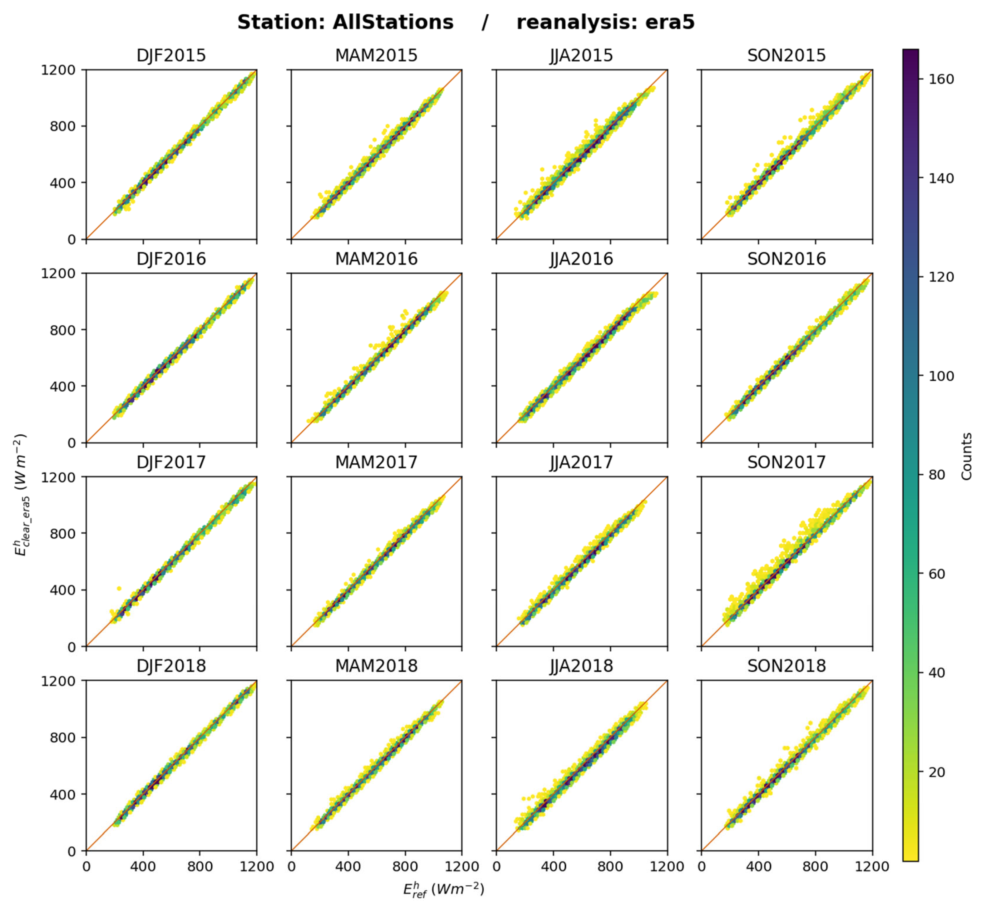
Figure 9 exhibits the 2D histograms between E r e f h and E c l e a r _ e r a 5 h for each trimester and all stations merged. A good overall fit is observed between the estimates and the reference: the points are well aligned along the 1:1 line with limited dispersion, except during SON2017. The correlation coefficients are greater than 0.979 at any station, for any trimester, and the slope of the fitting line ranges between 0.93 and 1.08 (as detailed in the Supplementary Materials). One may note in Figure 9 that there is a tendency to underestimation of E r e f h by E c l e a r _ e r a 5 h : the bias for all data merged is −11 W m−2.
Figure 10 exhibits the bias and its relative value with respect to the reference means in E h (Figure 5) at each station and all stations merged for each trimester and all trimesters merged. The bias ranges between −42 W m−2 and 27 W m−2. It is most often negative: among the 333 cases, 70% underestimate with a bias less than −5 W m−2, 17% have a bias in the interval [−5, 5] W m−2, and 13% a bias greater than 5 W m−2. Thirteen stations have a bias per trimester always less than −5 W m−2: TOR, LIN, CAB, PAL, PAY, CNR, LRC, MNM, ASP, FLO, DAA, GVN, and DOM. The largest negative biases for all trimesters merged are found at LIN (−28 W m−2), CAB, and ASP (both −25 W m−2). The bias has low variations from year to year or from season to season, except at FPE, SAP, and ASP. Though there are large variations in bias among stations, there is no visible relationship between the bias in E h and the latitude, or with the effective solar zenithal angle θ S e f f _ h . Notable changes in bias are observed with Köppen–Geiger climatic classes (Table 1), but no trend is visible.
Figure 11 exhibits the standard deviation of the differences ( E c l e a r _ e r a 5 h E r e f h ) and its relative value with respect to the reference means in E h (Figure 5) at each station and all stations merged for each trimester and all trimesters merged. The standard deviation per trimester ranges between 2 W m−2 and 44 W m−2. In 57% of the 333 cases, the standard deviation is less than 10 W m−2, and less than 20 W m−2 in 94%. The standard deviations at the two southernmost sites GVN and DOM are always less than 10 W m−2, while those at NYA, TOR, CAB, PAL, PAY, CAR, MNM, PTR, FLO, LAU, and SYO are always less than 15 W m−2. Standard deviations per trimester greater than 25 W m−2 are found at SAP, BOS, and GOB. In relative value, the standard deviation is less than 2% in 65% of the cases, and less than 3% in 90% of the cases. During a given season, the standard deviation has low variations from year to year, except at SAP and GOB. The contrast between seasons is weak in the southern hemisphere and more marked in the northern hemisphere, where values are among the greatest during MAM and JJA.
Figure 12 shows the 2D histograms between K T r e f h and K T c l e a r _ e r a 5 h for each trimester and all stations merged. As expected, the fit along the 1:1 line is not as good as for E c l e a r _ e r a 5 h but still it is quite good and the scatter is limited, except during SON2017, for which the bias is 0.01 and the standard deviation of differences is 0.03. The correlation coefficient between K T c l e a r _ e r a 5 h and K T r e f h per trimester is greater than 0.85 in most of the cases, with several lower values at SAP and DOM (see Supplementary Materials). One may note in Figure 12 that there is a tendency to the underestimation of K T r e f h by K T c l e a r _ e r a 5 h : the bias for all data merged is −0.016. Only 17% of the 333 cases exhibit a positive bias per trimester (see Supplementary Materials). The features of the biases and standard deviations per trimester per station for K T h are similar to those for E h (Figure 10 and Figure 11).
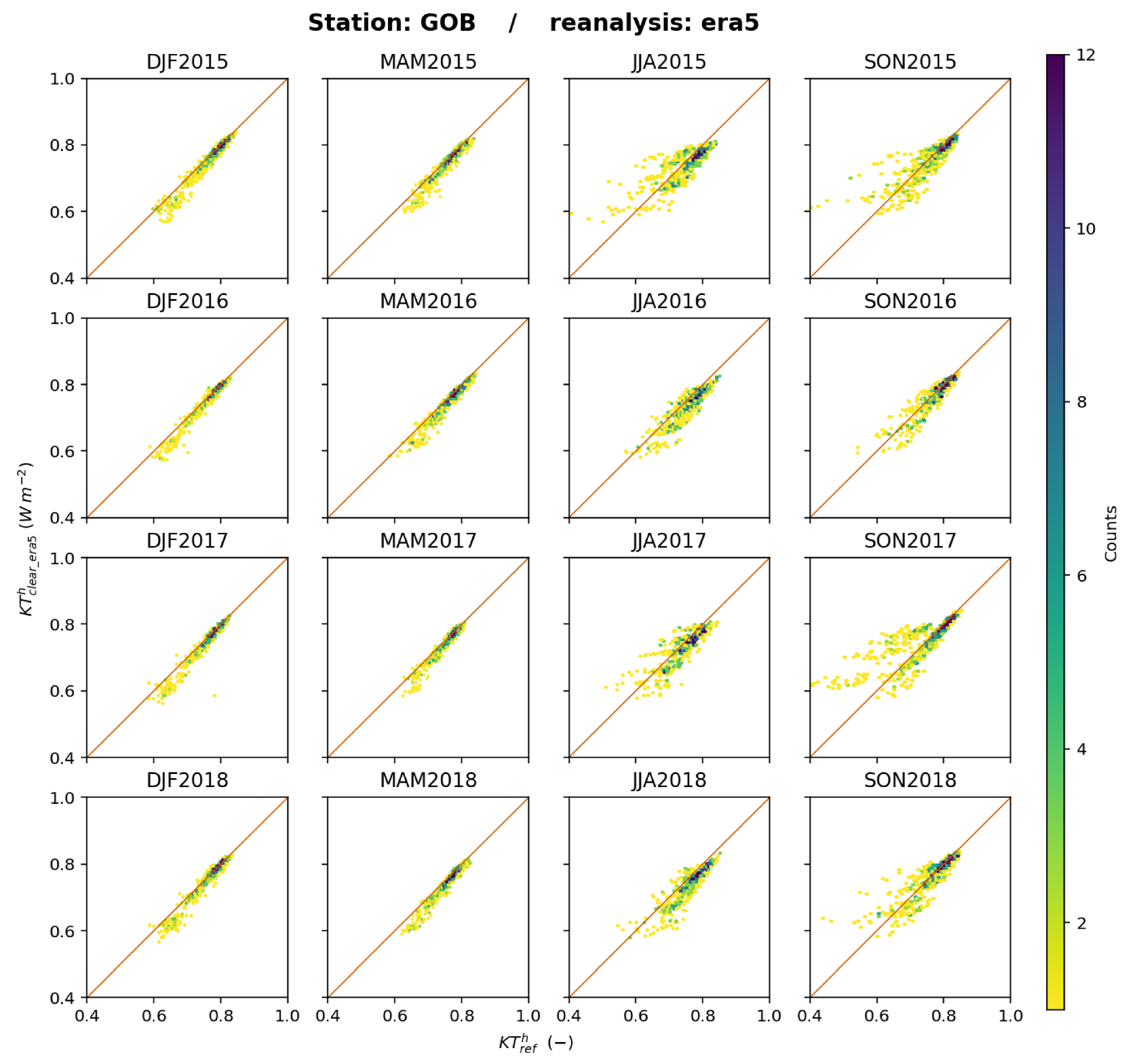
Such 2D histograms were drawn for each station and offer a great number of similarities (see Supplementary Materials). Figure 13 exhibits the 2D histograms between K T r e f h and K T c l e a r _ e r a 5 h at Gobabeb for each trimester as an example. Of particular interest here is the 2D histograms for JJA and SON. One may observe sorts of yellow horizontal lines that indicate that while K T r e f h varies, K T c l e a r _ e r a 5 h remains constant. This could reflect the influence of using a climatology that cannot reproduce the actual fluctuations in aerosol properties during this trimester, resulting in fluctuations in K T r e f h , which are not captured by ERA5.
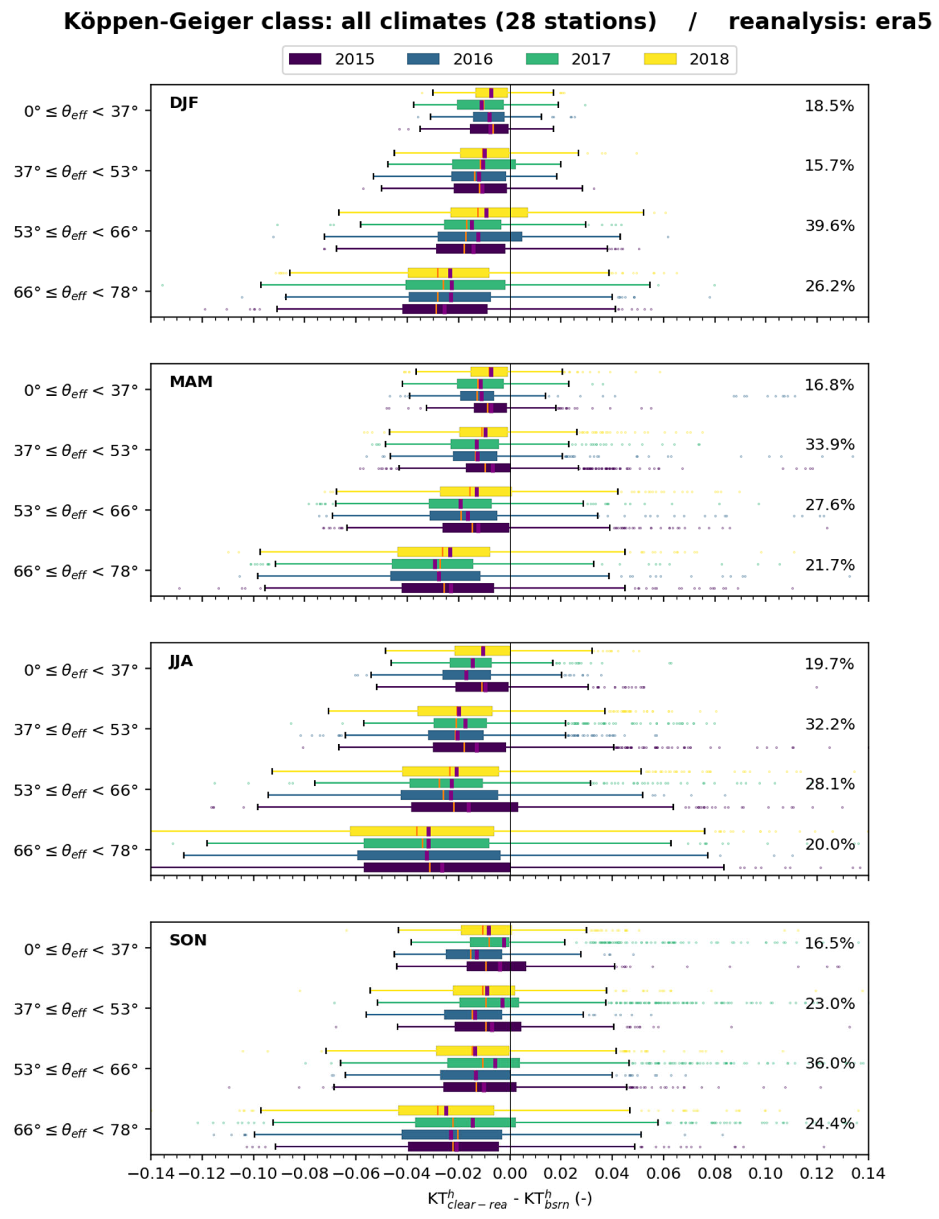
Figure 14 exhibits boxplots of the differences ( K T c l e a r _ e r a 5 h K T r e f h ) for all stations merged for several classes of θ S e f f _ h for each trimester. The bias in K T h is always negative in this graph. The bias and the standard deviation of the differences vary with θ S e f f _ h and the trimester. The bias is more and more negative and the standard deviation increases as θ S e f f _ h increases. This effect is most pronounced during JJA. Changes from year to year are limited and less marked than those from season to season.
No trend with climate can be detected visually on the bias and standard deviation. Whatever the climate, the differences are most often negative; the standard deviation remains fairly constant, and the bias exhibits more fluctuations. Boxplots for each climate, each season, and each year for the θ S e f f _ h classes exhibit complex patterns with no obvious trend. A thorough analysis is necessary and is beyond our investigative means.
Table 3 summarizes the bias, standard deviation of differences, and root mean square of differences (RMSD) in E h and K T h at each station and all stations merged for all trimesters merged. The relative bias in E h and K T h , respectively, is most often negative and ranges from −5% to 1% and −6% to 1%. The relative standard deviation in E h or K T h has low variations as it is most often in the range [2, 3]%.

6. Results for Clear-Sky Irradiance from JRA-3Q and Discussion

Figure 15 exhibits the 2D histograms between E r e f h and E c l e a r _ j r a 3 q h for each trimester and all stations merged. A good overall fit is observed between the estimates and the reference: the points are well aligned along the 1:1 line with limited dispersion. The correlation coefficients between E c l e a r _ j r a 3 q h and E r e f h are greater than 0.980 at any station for any trimester, and the slope of the fitting line ranges between 0.95 and 1.09, with a mean equal to 1.01 (see Supplementary Materials).
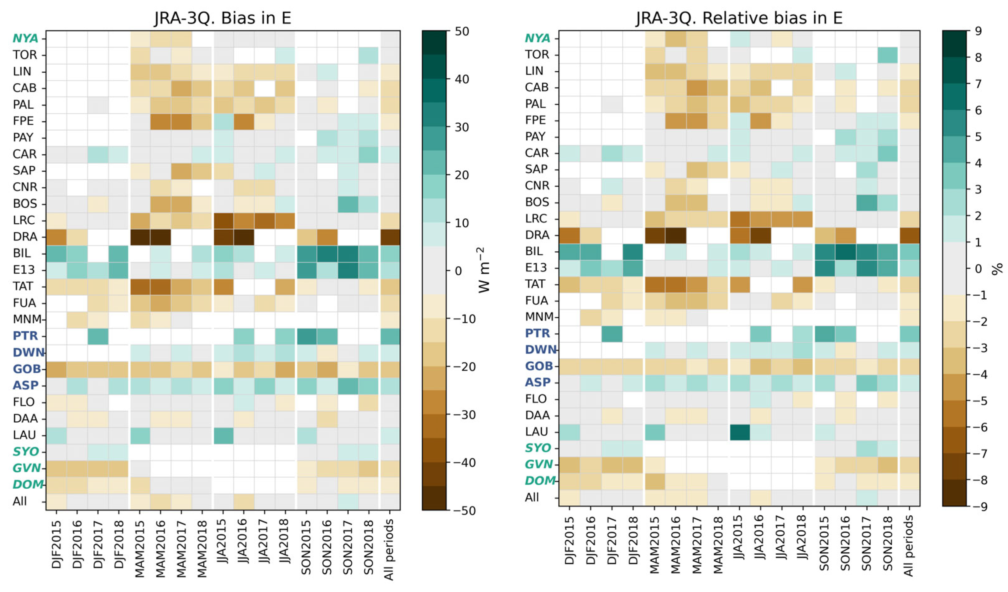
Figure 16 exhibits the bias and its relative value with respect to the reference means in E h (Figure 5) at each station and all stations merged for each trimester and all trimesters merged. The bias at Desert Rock (DRA) is always negative and very low, being between −13 W m−2 and −63 W m−2. Otherwise, the bias ranges between −36 W m−2 and 33 W m−2. The bias is in the range [−5, 5] W m−2 in 114 cases (34%), in the range [5, 33] W m−2 in 84 cases (25%), and less than −5 W m−2 in 135 cases (41%). BIL, E13, and PTR exhibit the greatest biases. At a given station and during a given trimester, the bias has low variations from year to year except at the stations in Northern America (FPE, LRC, DRA, BIL, and E13) and TAT. The biases exhibit large variations from trimester to trimester, and from station to station. There is no visible relationship between the bias in E h and the latitude, or with the effective solar zenithal angle θ S e f f _ h . Significant changes with Köppen–Geiger climatic classes (Table 1) are observed but no trend has been identified.
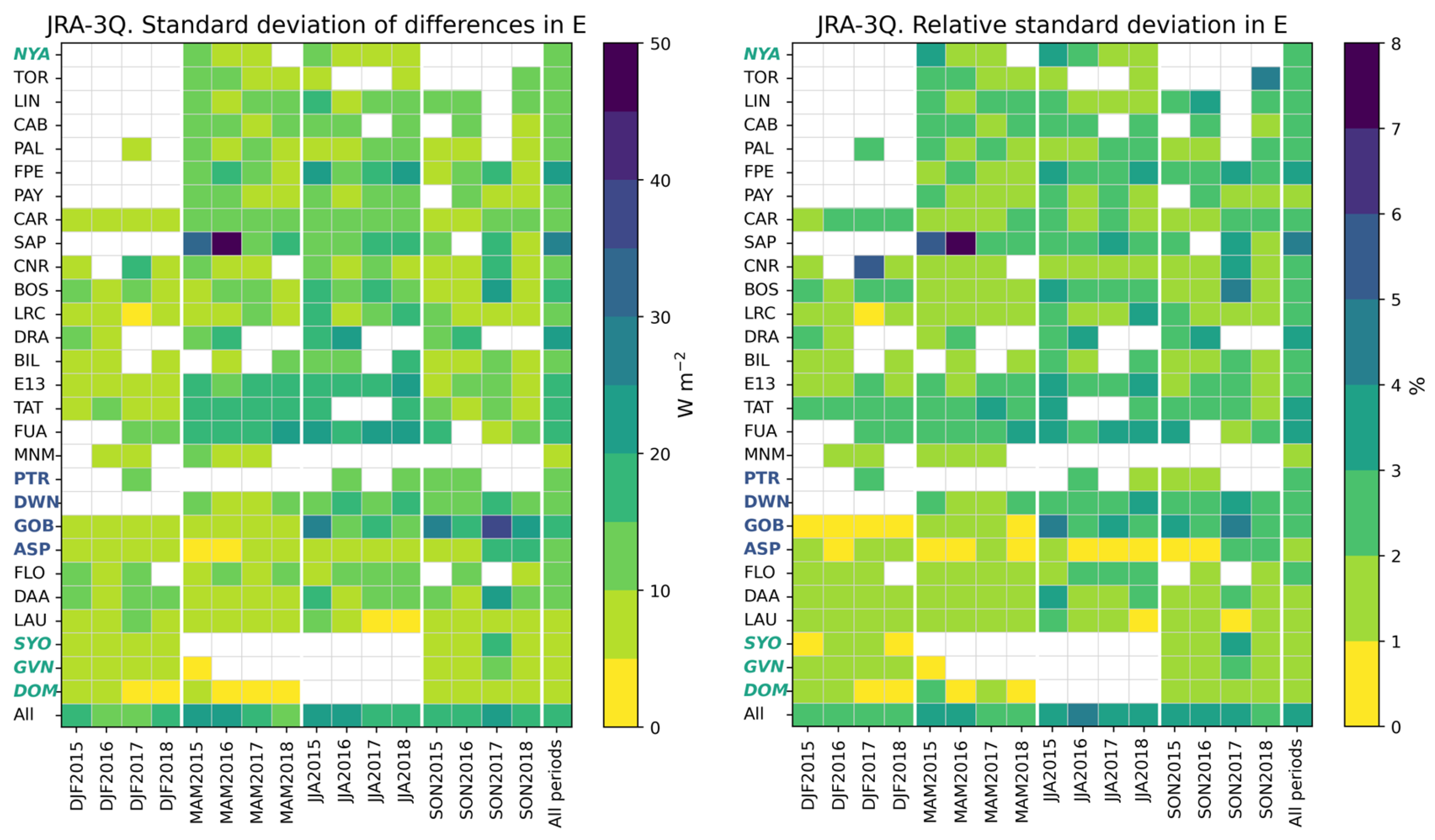
Figure 17 exhibits the standard deviation of the differences ( E c l e a r _ j r a 3 q h     E r e f h ) and its relative value with respect to the reference means in E h (Figure 5) at each station and all stations merged for each trimester and all trimesters merged. The standard deviation per trimester ranges between 3 W m−2 and 46 W m−2. In 54% of the 333 cases, the standard deviation is less than 10 W m−2, and less than 20 W m−2 in 96% of cases. MNM and the two southernmost sites GVN and DOM have standard deviations always less than 10 W m−2. Those at NYA, TOR, LIN, CAB, PAL, PAY, CAR, PTR, FLO, and LAU, are always less than 15 W m−2. Values greater than 25 W m−2 are found at SAP and GOB. In relative value, the standard deviation is less than 2% in 75% of the cases and less than 3% in 96% of the cases. During a given season, the standard deviation has low variations from year to year, except at SAP and GOB. The contrast between seasons is weak in the southern hemisphere and more marked in the northern hemisphere, where values are among the greatest during MAM and JJA.
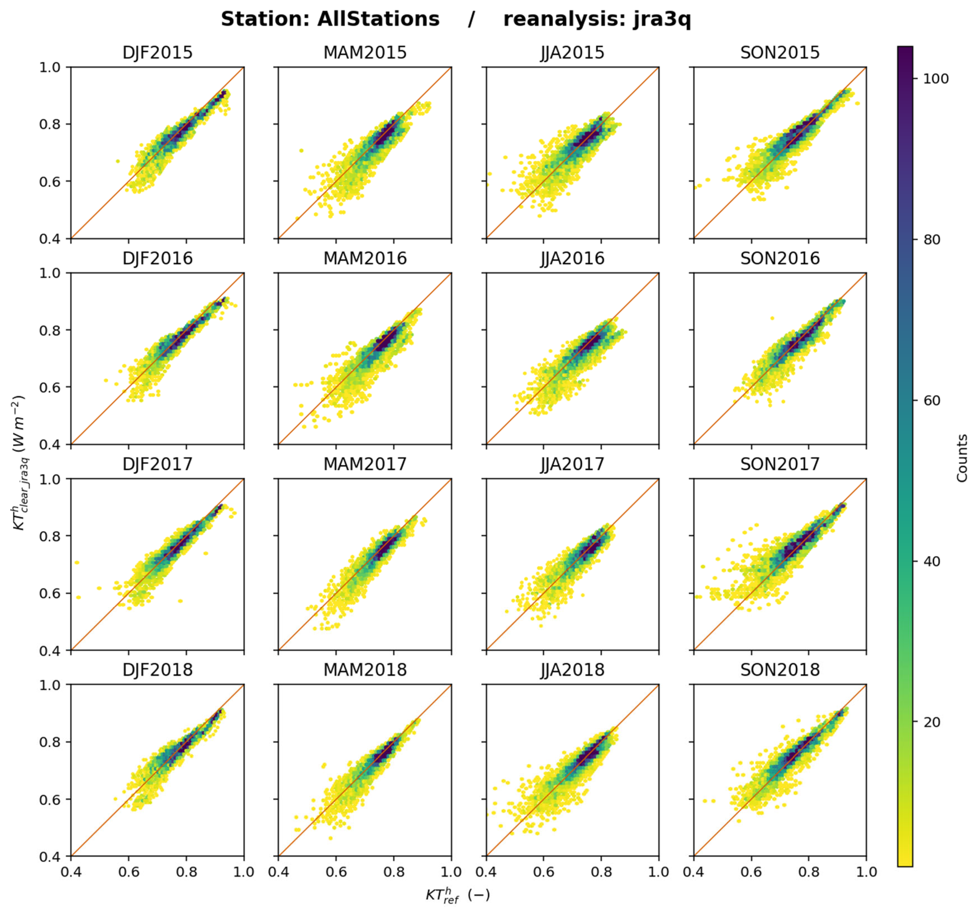
Figure 18 shows the 2D histograms between K T r e f h and K T c l e a r _ j r a 3 q h for each trimester and all stations merged. The fit along the 1:1 line is quite good though not as good as for E c l e a r _ j r a 3 q h . The scatter varies from trimester to trimester and is systematically high during JJA. The correlation coefficient between K T c l e a r _ j r a 3 q h and K T r e f h per trimester is greater than 0.85 in most of the cases. Very low values are found at CNR during DJF2017 (0.672) and DOM during MAM2017 (0.481) (see Supplementary Materials). The slope per trimester (see Supplementary Materials) is comprised between 0.95 and 1.05 in 24% of the cases. It is greater than 1.05 in 33% of the cases and less than 0.95 in 43% of the cases.
The bias in K T h per trimester (see Supplementary Materials) is close to 0 overall: 41% of the cases are in the range [−0.01, 0.01], 18% are greater than 0.01, 18% in the range [−0.02, −0.01], and 23% are less than −0.02. The bias is always less than −0.01 at CAB, DRA, and SYO and always greater than 0.01 at BIL and PTR. It varies from station to station, trimester to trimester, and year to year. The features of the biases and standard deviations per trimester per station for K T h are similar to those for E h (Figure 16 and Figure 17).
Two-dimensional histograms were drawn at each station and offer a great number of similarities (see Supplementary Materials). Figure 19 exhibits the 2D histograms between K T r e f h and K T c l e a r _ j r a 3 q h at Gobabeb for each trimester as an example. During JJA and SON, one may observe sorts of yellow quasi-horizontal lines (see e.g., JJA2015 for K T c l e a r _ j r a 3 q h = 0.6 ) that indicate that while K T r e f h varies, K T c l e a r _ j r a 3 q h remains constant. This could reflect the influence of using a climatology for aerosols, which cannot reproduce the actual fluctuations in aerosol optical properties during this trimester, resulting in fluctuations in K T r e f h , which are not captured by JRA-3Q.
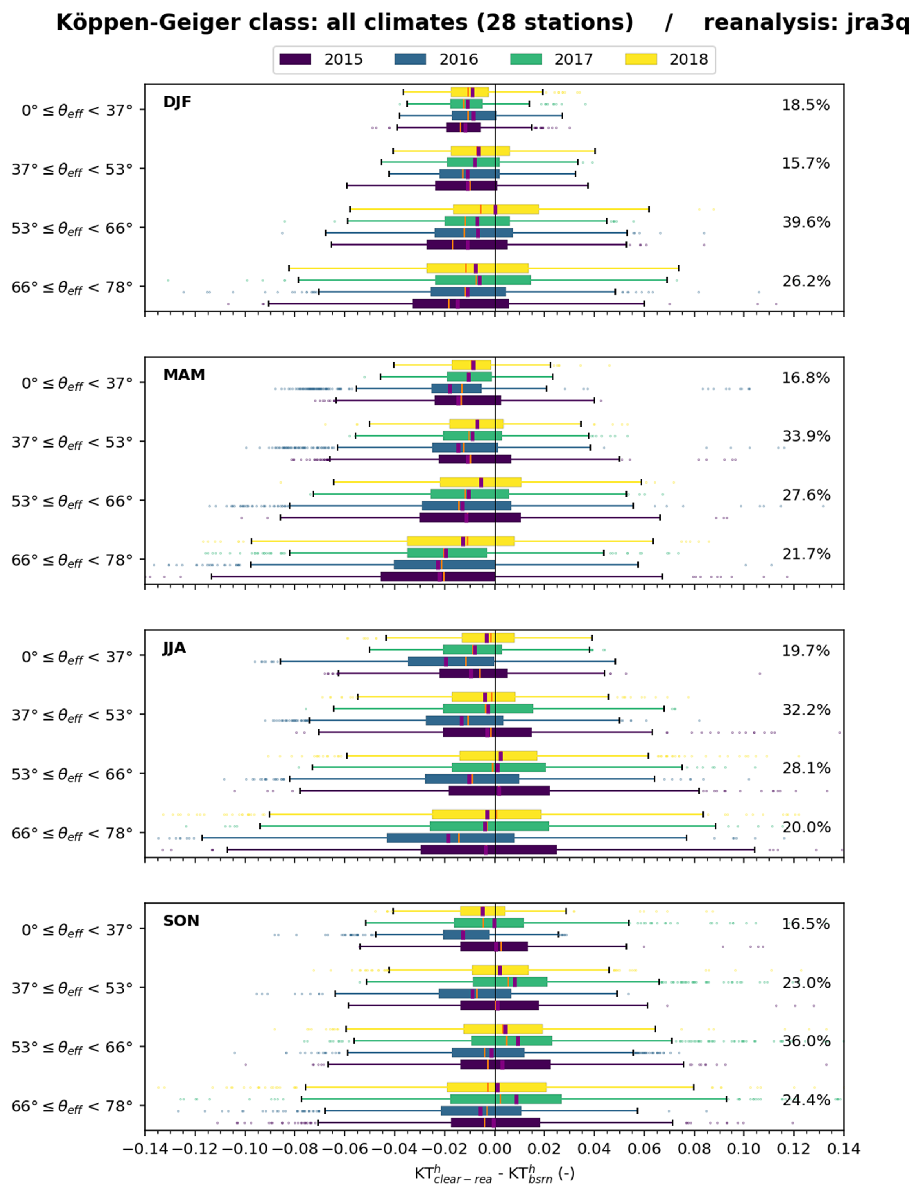
Figure 20 exhibits boxplots of the differences ( K T c l e a r _ j r a 3 q h K T r e f h ) for all stations merged for several classes of θ S e f f _ h for each trimester. During a given year and a given season, changes in bias with θ S e f f _ h are limited while the standard deviation increases as θ S e f f _ h increases. During DJF and MAM, differences are most often negative whatever the value of θ S e f f _ h , meaning an underestimation of K T r e f h by K T c l e a r _ j r a 3 q h . Changes from year to year are limited during these seasons. During JJA and SON, differences are more centered on 0 for all years but 2016, which tends to be more negative. Other graphs show that the bias and standard deviation for each class of θ S e f f _ h fluctuate between stations; no trend with latitude or climate can be detected visually.
Boxplots for each climate, each season, and each year for the θ S e f f _ h classes exhibit complex patterns with no obvious trend. For each possible class, the differences may be low or high, negative or positive. Biases fluctuate significantly; standard deviations tend to increase as θ S e f f _ h increases.
Table 4 summarizes the bias, standard deviation of differences, and root mean square of differences (RMSD) in E h and K T h at each station and all stations merged for all trimesters merged. The relative bias in E h and K T h , respectively, ranges from −6% to 4% and −7% to 4%. The relative standard deviation in E h or K T h has low variations as it is often in the range [2, 3]%.

7. Results for Clear-Sky Irradiance from MERRA-2 and Discussion

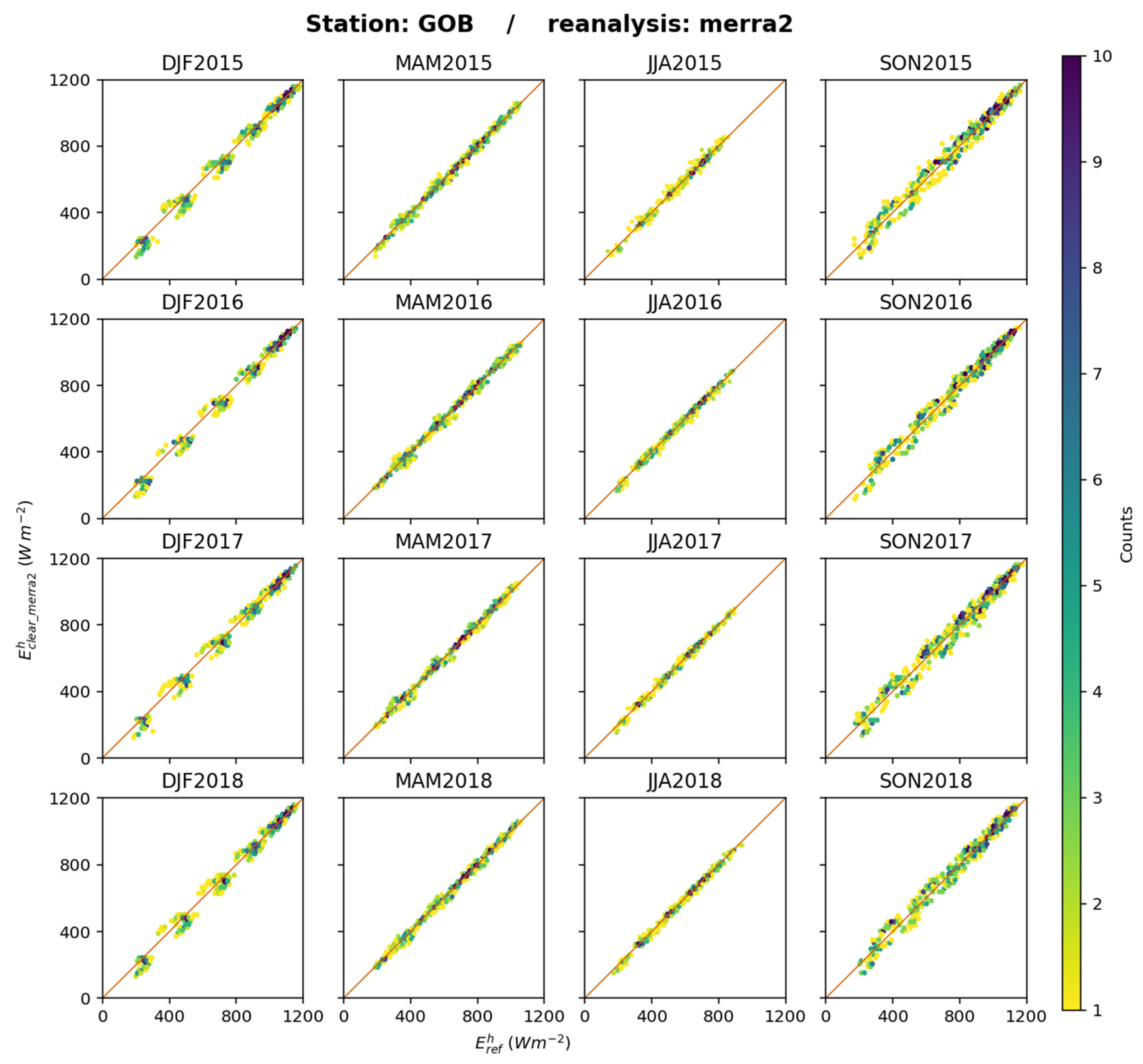
The results for MERRA-2 regarding E h are affected by the mismatch in time system at intraday scales and, therefore, by a miscalculation of the solar zenithal angle θ s . This miscalculation is propagated to the irradiance at the top of the atmosphere, E 0 _ m e r r a 2 h , and also to the clear-sky SIS E c l e a r _ m e r r a 2 h and clearness index K T c l e a r _ m e r r a 2 h due to the dependence of absorption and scattering by atmospheric constituents on θ s . Figure 21 exhibits the 2D histograms between E r e f h and E c l e a r _ m e r r a 2 h for each trimester and all stations merged. Overall, the points are well aligned along the 1:1 line. The slope of the fitting line per trimester per station ranges between 0.91 and 1.11 but ranges between 0.95 and 1.05 in most cases (see Supplementary Materials). The dispersion of the most populated classes (green and blue) along the 1:1 line is noticeable during DJF and SON and is limited during MAM and JJA. This is only a general feature when all stations are merged and the actual situation varies from station to station. Similar 2D histograms at each station are given in the Supplementary Materials. As an example, Figure 22 exhibits the 2D histograms between E r e f h and E c l e a r _ m e r r a 2 h for each trimester at Gobabeb. One may observe during DJF that the dots are not well distributed along the 1:1 line and form horseshoe-shaped spots along this line that are typical of the time system mismatch.
Figure 23 displays the correlation coefficients per trimester per station. They are greater than 0.967 but many of them (14%) are less than 0.985. The coefficients exhibit a pattern that has seasonal and latitudinal dependency. The smallest are observed in the northern hemisphere during DJF and SON to a lesser extent and during MAM at the South Pole. This pattern in time and space originates from the mismatch in time system and can affect intraday calculations.
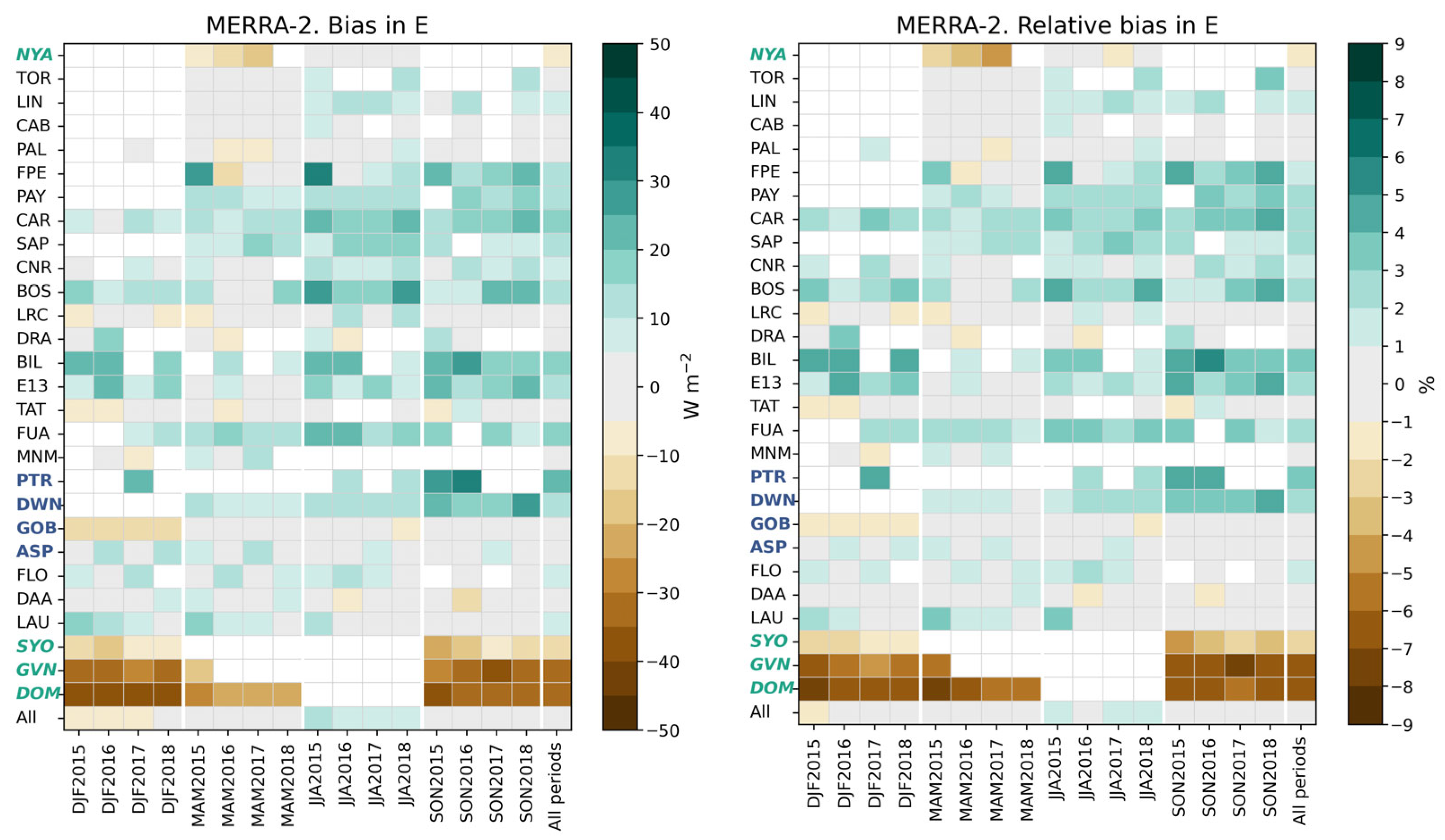
The bias and its relative value with respect to the reference means in E h (Figure 5) at each station and all stations merged for each trimester and all trimesters merged are displayed in Figure 24. The bias ranges between −39 W m−2 and 34 W m−2. It is in the interval [−5, 5] W m−2 in 35% of the cases; 16% have a bias less than −5 W m−2, 49% a bias greater than 5 W m−2, and 17% a bias greater than 15 W m−2. As a whole, the bias at a given station during a given trimester does not vary much with the year. It varies more from trimester to trimester and from station to station. The two southernmost stations have large negative biases, less than −15 W m−2, during all trimesters. Except for these stations, there is no clear relationship between the bias in E h and the latitude, though one may note that the stations between 49° and 58° (TOR, LIN, CAB, and PAL) and between −23° and −45° (GOB, ASP, FLO, DAA, and LAU) have low relative biases, mostly comprised between −2% and 2%, with no clear link with Köppen–Geiger climatic classes (Table 1).
Figure 25 exhibits the standard deviation of the differences ( E c l e a r _ m e r r a 2 h     E r e f h ) and its relative value with respect to the reference means in E r e f h (Figure 5) at each station and all stations merged for each trimester and all trimesters merged. The standard deviation per trimester ranges between 5 W m−2 and 43 W m−2. It is large as a whole: it is less than 10 W m−2 in only 5% of the 333 cases. It lies in the range [10, 20] W m−2 in 57% of the cases, in the range [20, 30] W m−2 in 24% of the cases, and is greater than 30 W m−2 in 14% of the cases. In relative value, the standard deviation is less than 2% in only 9% of the cases. It is in the range [2, 3]% in 34% of the cases, in the range [3, 4]% in 20% of the cases, and greater than 4% in 23% of the cases. There is no clear picture between the standard deviation and latitude or station or climate. What is clear is the increase in the standard deviation during DJF and SON compared to MAM and JJA. This is to be related to the similar pattern discussed in Figure 23, which is attributed to the mismatch in time system.
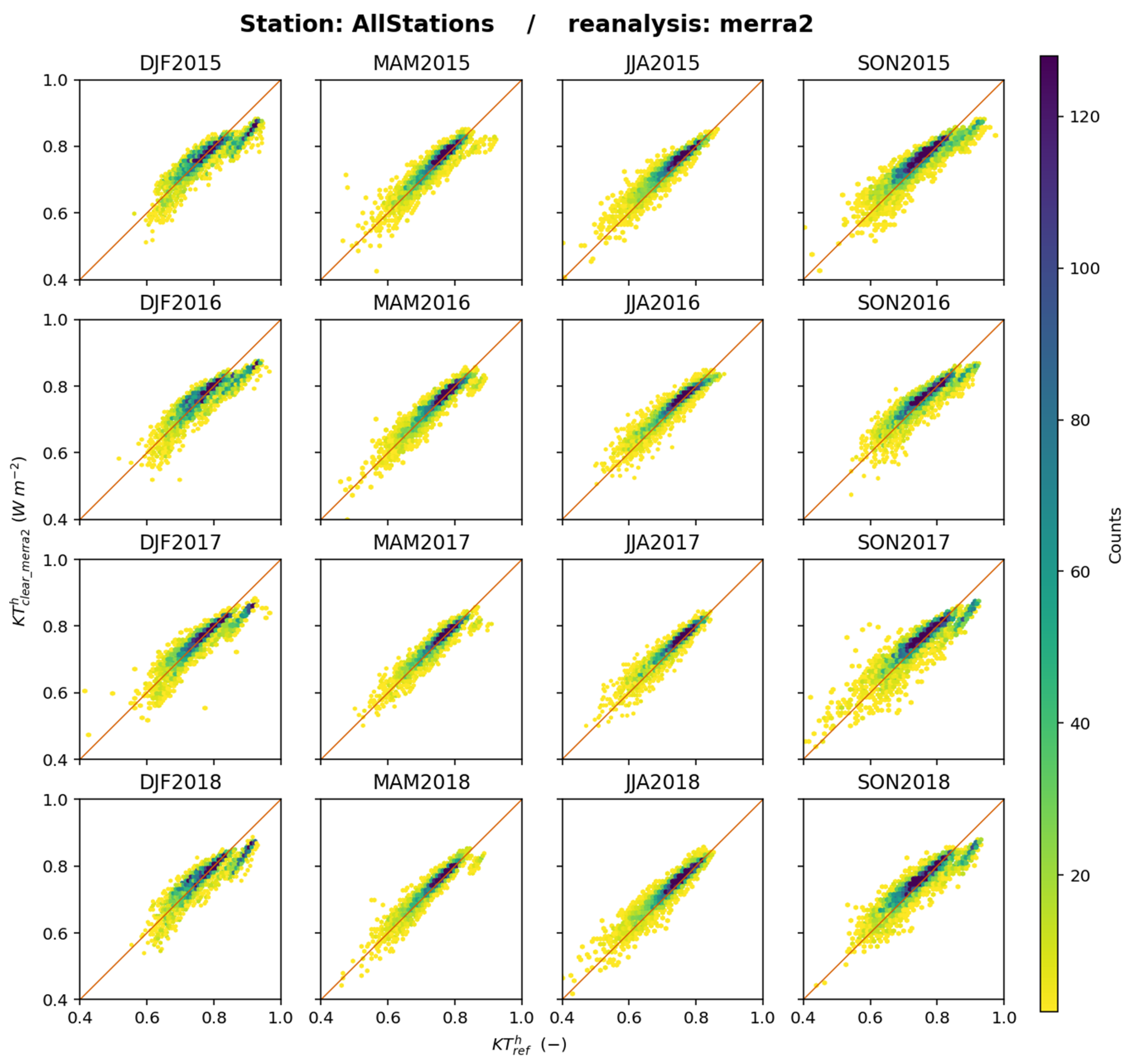
Figure 26 shows the 2D histograms between K T r e f h and K T c l e a r _ m e r r a 2 h for each trimester and all stations merged. As expected, the fit along the 1:1 line is not as good as for E c l e a r _ m e r r a 2 h but it is still quite good and the scatter is limited. One may note during DJF, JJA, and SON, a group of dots of high K T r e f h that lies well below the 1:1: line. This group is due to the southernmost stations: SYO, GVN, and DOM, for which the bias is largely negative, being, respectively, −0.02, −0.05, and −0.06 when averaged over all trimesters. The northernmost station NYA, also in a polar climate, also has a negative bias of −0.01 on average. These four stations have the most noticeable negative biases averaged over all trimesters; the other stations exhibit biases close to 0 or with positive values of up to 0.02 (Table 5), as illustrated in Figure 26. It may be hypothesized that these negative biases are partly due to incomplete consideration of the high albedo surfaces surrounding the sites, though the authors do not have the details of the calculation of K T c l e a r _ m e r r a 2 h , and other reasons are possible. Among them, one can think of measurement issues due to frozen pyranometers [42] not detected by quality control, although measurement issues cannot be the major reason as they should also affect the results for ERA5 and JRA-3Q, which do not exhibit behaviours at polar stations similar to those for MERRA-2.
The correlation coefficient between K T c l e a r _ m e r r a 2 h and K T r e f h per trimester is greater than 0.85 in most of the cases (see Supplementary Materials). This coefficient does not exhibit the same pattern as that between E c l e a r _ m e r r a 2 h and E r e f h (Figure 23) as the effect of the diurnal cycle of E 0 _ m e r r a 2 h is removed in K T c l e a r _ m e r r a 2 h and this mitigates the effects of the mismatch in time system.
Similar 2D histograms were drawn at each station and offer a great number of similarities (see Supplementary Materials). As an example, Figure 27 exhibits the 2D histograms between K T r e f h and K T c l e a r _ m e r r a 2 h at Gobabeb for each trimester. Of particular interest here is the 2D histogram for SON2017, which can be compared to those obtained for ERA5 (Figure 13) and JRA-3Q (Figure 19) on which sorts of yellow quasi-horizontal lines indicate that while K T r e f h varies, K T c l e a r _ e r a 5 h and K T c l e a r _ j r a 3 q h , respectively, remain constant, reflecting the influence of using a climatology. MERRA-2 does not exhibit such a pattern and captures the actual fluctuations in K T r e f h , though the scatter cannot be neglected. This could be attributed to the assimilation of aerosols’ properties in MERRA-2.
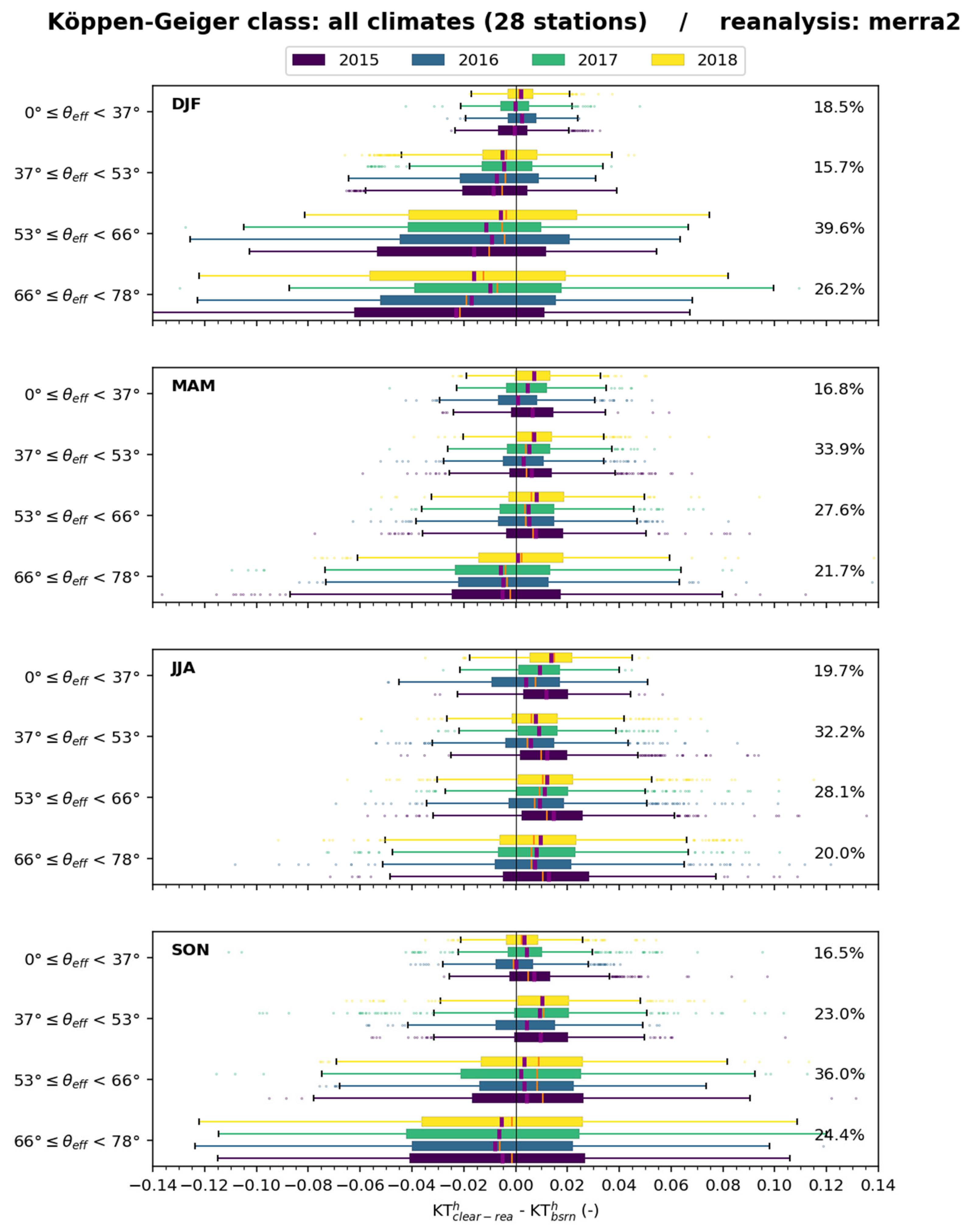
Figure 28 exhibits boxplots of the differences ( K T c l e a r _ m e r r a 2 h K T r e f h ) for all stations for several classes of θ S e f f _ h for each trimester. Changes from year to year are limited for a given trimester. The bias and the standard deviation of the differences vary with θ S e f f _ h and the trimester. During DJF, the bias is negative and decreases as θ S e f f _ h increases. The differences are most often negative, meaning a very frequent underestimation of K T r e f h by K T c l e a r _ m e r r a 2 h . The pattern is fairly similar during SON, and, to a lesser extent, MAM, though the bias is positive, except at the greatest θ S e f f _ h , and differences are more balanced between negative and positive values. During JJA, the bias is always positive with no influence of θ S e f f _ h ; K T c l e a r _ m e r r a 2 h very frequently overestimates K T r e f h . During each trimester, the standard deviation increases with θ S e f f _ h .
Boxplots for each climate, each season, and each year for the θ S e f f _ h classes exhibit complex patterns; no trend can be visually detected, except at the polar stations, as already reported. Whatever the climate, the differences are frequently positive. They sometimes fluctuate with the year or with θ S e f f _ h . Standard deviations tend to increase with θ S e f f _ h . A deeper analysis of the links between differences, climate, and θ S e f f _ h is beyond our investigative means.
Table 5 summarizes the bias, standard deviation of differences, and root mean square of differences (RMSD) in E h and K T h at each station and all stations merged for all trimesters merged. The relative biases in E h and K T h are often positive and range from −7% to 4%. The relative standard deviation in E h or K T h has fairly low variations as it is often in the range [3, 4]%.

8. Conclusions

The present work has compared estimates of the hourly means in clear-sky conditions provided by the ERA5, JRA-3Q, and MERRA-2 reanalyses against coincident ground-based measurements from 28 BSRN stations covering four years (2015–2018) in an attempt to identify strengths and potential drawbacks in the modelling of E c l e a r h and to inform the agencies in charge of the reanalyses of further developments as uncertainties in E c l e a r h affect the estimates of the SIS in all conditions. It is stressed here that the presented work deals with hourly values E c l e a r _ e r a 5 h , E c l e a r _ j r a 3 q h , and E c l e a r _ m e r r a 2 h , thus complementing the studies already mentioned, dedicated to the analysis of daily and monthly means of SIS under clear-sky conditions.
The 28 stations are located worldwide but still cover a limited number of climates and a limited number of geographical and meteorological conditions. The BSRN measurements are 1-min measurements and were processed to identify clear-sky conditions. The selected measurements were then aggregated into hourly clear-sky irradiance E r e f h . These processes decrease the information content of the initial 1-min BSRN measurements to a limited extent, but they are necessary to match the temporal resolution of the reanalysis.
It was found that ERA5 very frequently underestimates E r e f h . The bias per trimester per station ranges from −7% to 5%, relative to the corresponding average in E r e f h . The relative biases are most often negative: 70% of them are less than −1% and 52% are less than −2%. The bias varies little from one year to another and from one trimester to another at a given station, but, significantly, from one station to another. As a whole, the differences ( E c l e a r _ e r a 5 h     E r e f h ) tend to be more and more negative as the effective solar zenithal angle θ S e f f _ h increases. The fidelity or consistency to E r e f h is satisfactory as fluctuations in time are well captured by ERA5 with little dispersion: the correlation coefficients are very high and the standard deviations of differences per trimester relative to the corresponding average in E r e f h are fairly constant in time and across stations and are small: they are less than 2% in 60% of the cases, and less than 3% in 90% of the cases. From our results, we conclude that ERA5 can be considered as fairly reliable in time, despite its use of an aerosol climatology, i.e., it offers the same level of uncertainty because the statistical indicators do not fluctuate significantly with time at a given station. However, we observed that this is not true at certain locations, such as Gobabeb, where the use of a climatology leads to notable fluctuations in statistical indicators over time. In contrast, ERA5 is not reliable in space because of the large fluctuations in bias from station to station.
Our results suggest some areas for improving estimates of the hourly means in clear-sky conditions provided by ERA5. Further analyses are necessary to understand why E c l e a r _ e r a 5 h so frequently underestimates E r e f h and the reasons for the spatial variability of the bias. In particular, experiments could be conducted to assess whether the aerosol climatology alone explains the underestimation and its fluctuations in space. Another hypothesis to be tested is whether the underestimation is partly due to a systematic underestimation of the ground albedo.
As for JRA-3Q, the bias per trimester per station ranges from −9% to 6%, relative to the corresponding average in E r e f h . Values are fairly well balanced between negative and positive values: 28% of the cases are in the range [−3, −1]%, 34% in [−1, 1]%, and 19% in [1, 3]%. The bias most often exhibits low variations from year to year but large variations across trimesters and stations are observed. Fluctuations in time are well captured by JRA-3Q: the correlation coefficients are very high. The standard deviations of differences per trimester relative to the corresponding average in E r e f h are small: they are less than 2% in 75% of the cases and less than 3% in 96% of the cases. Most often, the standard deviation has low variations across stations and years during a given season. In contrast, changes across seasons are weak in the southern hemisphere and significant in the northern hemisphere. Despite the low values of the standard deviations, these possible changes with the season do not guarantee a good fidelity to E r e f h . No significant overall trend with θ S e f f _ h was observed. From our results, we conclude that JRA-3Q is not reliable in time or space because of the large changes in bias and, sometimes, standard deviation from one station to another and from one trimester to another.
Our results suggest, as for ERA5, that additional analyses should be conducted to understand the origin of spatial and seasonal variations in bias and potentially identify ways to improve the model. One could also assess the impact of using aerosol climatology on the uncertainty of clear-sky estimates, especially to evaluate whether the observed differences in standard deviation and bias between regions and seasons can be explained by the use of a climatology.
The results for MERRA-2 regarding E h are strongly affected by the use of the mean solar time instead of the true solar time, which leads to a miscalculation of the solar zenithal angle θ s . This miscalculation is propagated to the irradiance at the top of the atmosphere, E 0 _ m e r r a 2 h , and also to the clear-sky SIS E c l e a r _ m e r r a 2 h and clearness index K T c l e a r _ m e r r a 2 h due to the dependence of absorption and scattering by atmospheric constituents on θ s . Among many examples of this influence on the statistical indicators, the correlation coefficients exhibit a pattern that has seasonal and latitudinal dependency that can affect intraday calculations. At a given station during a given trimester, the bias does not vary much with the year. It varies more across trimesters and stations. Only 43% of the cases have a relative standard deviation less than 3% and 23% of them have values greater than 4%. The standard deviation exhibits a marked seasonal pattern with an overall increase during DJF and SON compared to MAM and JJA. The standard deviation increases with θ S e f f _ h while the link between the bias and θ S e f f _ h is more complex and depends on the season. From our results, we conclude that MERRA-2 is not reliable in time or space because of the large changes in statistical indicators from one station to another and from one trimester to another.
Our recommendations for improving estimates of the hourly means in clear-sky conditions provided by MERRA-2 are as follows. Correct the time system. This should improve all statistical indicators. A study similar to this one may then reveal some features whose analysis can lead to further improvements. Attention should be paid to the extreme latitudes as the four polar stations exhibit the most noticeable negative biases compared to the other stations.
This work exposes the strengths and weaknesses of each reanalysis in clear-sky conditions and formulates suggestions for further improvements in the estimates of the hourly means of irradiance E c l e a r h in such conditions. Currently, none of the three studied reanalyses is satisfactory in cloud-free conditions and all are far from matching the quality of advanced models dedicated to the estimates of E c l e a r h such as CAMS-McClear and others, as reported in recent papers [19,28].
In addition to the assessment of the hourly means in clear-sky conditions provided by the ERA5, JRA-3Q, and MERRA-2 reanalyses, this paper has presented a new algorithm for detecting cloud-free instants that produces similar results to two other equivalent methods. This new algorithm requires further analysis to rigorously assess its strengths and limitations. This will be addressed in a separate article specifically dedicated to this investigation.

Supplementary Materials

The following supporting information can be downloaded at: https://www.mdpi.com/article/10.3390/atmos16080949/s1, Figure S1: Bias, standard deviation of error, root mean square error, and slope of the three reanalyses for the variable E, analysed by trimester and station. Figure S2: Bias, standard deviation of error, root mean square error, and slope of the three reanalyses for the variable KT, by trimester and station. Figure S3: Scatterplots of reference versus analysis values of E for the three reanalyses, presented separately for individual stations as well as for the merged dataset of all stations. Figure S4: Scatterplots of reference versus analysis values of KT for the three reanalyses, presented separately for individual stations as well as for the merged dataset of all stations. Figure S5: Boxplots of the differences between reanalysis and reference values of E, shown for each individual station and for all stations combined, categorized by several classes of effective solar zenith angle θ S e f f _ h for each trimester. Figure S6: Boxplots of the differences between reanalysis and reference values of KT, shown for each individual station and for all stations combined, categorized by several classes of effective solar zenith angle θ S e f f _ h for each trimester.

Author Contributions

Conceptualization, methodology, validation, formal analysis, and visualization, Y.-M.S.-D. and L.W.; software, investigation, resources, data curation, supervision, project administration, and funding acquisition, Y.-M.S.-D.; writing—original draft preparation, L.W.; and writing—review and editing, Y.-M.S.-D. and L.W. All authors have read and agreed to the published version of the manuscript.

Funding

This research received no external funding.

Data Availability Statement

The BSRN measurements used in this study are available either via the BSRN FTP server (https://bsrn.awi.de/data/data-retrieval-via-ftp/, accessed on 11 July 2025) or through our institutional THREDDS data server (https://tds.webservice-energy.org/thredds/catalog/bsrn-stations/catalog.html, accessed on 11 July 2025). The reanalysis datasets are openly accessible: ERA5 was downloaded from the ECMWF Copernicus Climate Data Store (CDS), JRA-3Q from the THREDDS data server operated by UCAR, and MERRA-2 from the NASA Earthdata website.

Acknowledgments

The authors thank all operators of the ground stations of the BSRN network for their valuable measurements and the Alfred-Wegener Institute for hosting the BSRN website. We also acknowledge the institutions responsible for producing and maintaining the reanalysis datasets used in this study, namely ECMWF for ERA5, NASA GMAO for MERRA-2, and the Japan Meteorological Agency (JMA) for JRA-3Q.

Conflicts of Interest

The authors declare no conflicts of interest.

References

  1. Bojinski, S.; Verstraete, M.; Peterson, T.C.; Richter, C.; Simmons, A.; Zemp, M. The Concept of Essential Climate Variables in Support of Climate Research, Applications, and Policy. Bull. Am. Meteorol. Soc. 2014, 95, 1431–1443. [Google Scholar] [CrossRef]
  2. Lean, J.; Rind, D. Climate Forcing by Changing Solar Radiation. J. Clim. 1998, 11, 3069–3094. [Google Scholar] [CrossRef]
  3. Group on Earth Observations. GEO Task US-09-01a: GEO User Requirements for Air Quality Report; Group on Earth Observations: Geneva, Switzerland, 2013. [Google Scholar]
  4. Dantas De Paula, M.; Gómez Giménez, M.; Niamir, A.; Thurner, M.; Hickler, T. Combining European Earth Observation Products with Dynamic Global Vegetation Models for Estimating Essential Biodiversity Variables. Int. J. Digit. Earth 2020, 13, 262–277. [Google Scholar] [CrossRef]
  5. Group on Earth Observations. The GEOSS Water Strategy: From Observations to Decisions; Group on Earth Observations: Geneva, Switzerland, 2014. [Google Scholar]
  6. Ranchin, T.; Trolliet, M.; Ménard, L.; Wald, L. Which Variables Are Essential for Renewable Energies? Int. J. Digit. Earth 2020, 13, 253–261. [Google Scholar] [CrossRef]
  7. Juzeniene, A.; Brekke, P.; Dahlback, A.; Andersson-Engels, S.; Reichrath, J.; Moan, K.; Holick, M.F.; Grant, W.B.; Moan, J. Solar Radiation and Human Health. Rep. Prog. Phys. 2011, 74, 066701. [Google Scholar] [CrossRef]
  8. Lefevre, M.; Blanc, P.; Espinar, B.; Gschwind, B.; Menard, L.; Ranchin, T.; Wald, L.; Saboret, L.; Thomas, C.; Wey, E. The HelioClim-1 Database of Daily Solar Radiation at Earth Surface: An Example of the Benefits of GEOSS Data-CORE. IEEE J. Sel. Top. Appl. Earth Obs. Remote Sens. 2014, 7, 1745–1753. [Google Scholar] [CrossRef]
  9. Wald, L. Fundamentals of Solar Radiation, 1st ed.; CRC Press: Boca Raton, FL, USA, 2021; ISBN 978-1-003-15545-4. [Google Scholar]
  10. Hersbach, H.; Bell, B.; Berrisford, P.; Hirahara, S.; Horányi, A.; Muñoz-Sabater, J.; Nicolas, J.; Peubey, C.; Radu, R.; Schepers, D.; et al. The ERA5 Global Reanalysis. Q. J. R. Meteorol. Soc. 2020, 146, 1999–2049. [Google Scholar] [CrossRef]
  11. Kobayashi, S.; Ota, Y.; Harada, Y.; Ebita, A.; Moriya, M.; Onoda, H.; Onogi, K.; Kamahori, H.; Kobayashi, C.; Endo, H.; et al. The JRA-55 Reanalysis: General Specifications and Basic Characteristics. J. Meteorol. Soc. Jpn. 2015, 93, 5–48. [Google Scholar] [CrossRef]
  12. Kosaka, Y.; Kobayashi, S.; Harada, Y.; Kobayashi, C.; Naoe, H.; Yoshimoto, K.; Harada, M.; Goto, N.; Chiba, J.; Miyaoka, K.; et al. The JRA-3Q Reanalysis. J. Meteorol. Soc. Jpn. 2024, 102, 49–109. [Google Scholar] [CrossRef]
  13. Gelaro, R.; McCarty, W.; Suárez, M.J.; Todling, R.; Molod, A.; Takacs, L.; Randles, C.A.; Darmenov, A.; Bosilovich, M.G.; Reichle, R.; et al. The Modern-Era Retrospective Analysis for Research and Applications, Version 2 (MERRA-2). J. Clim. 2017, 30, 5419–5454. [Google Scholar] [CrossRef]
  14. Oumbe, A.; Qu, Z.; Blanc, P.; Lefèvre, M.; Wald, L.; Cros, S. Decoupling the Effects of Clear Atmosphere and Clouds to Simplify Calculations of the Broadband Solar Irradiance at Ground Level. Geosci. Model Dev. 2014, 7, 1661–1669. [Google Scholar] [CrossRef]
  15. Wang, Z.; Zhang, M.; Wang, L.; Feng, L.; Ma, Y.; Gong, W.; Qin, W. Long-Term Evolution of Clear Sky Surface Solar Radiation and Its Driving Factors over East Asia. Atmos. Environ. 2021, 262, 118661. [Google Scholar] [CrossRef]
  16. Trolliet, M.; Walawender, J.P.; Bourlès, B.; Boilley, A.; Trentmann, J.; Blanc, P.; Lefèvre, M.; Wald, L. Downwelling Surface Solar Irradiance in the Tropical Atlantic Ocean: A Comparison of Re-Analyses and Satellite-Derived Data Sets to PIRATA Measurements. Ocean Sci. 2018, 14, 1021–1056. [Google Scholar] [CrossRef]
  17. Lefèvre, M.; Oumbe, A.; Blanc, P.; Espinar, B.; Gschwind, B.; Qu, Z.; Wald, L.; Schroedter-Homscheidt, M.; Hoyer-Klick, C.; Arola, A.; et al. McClear: A New Model Estimating Downwelling Solar Radiation at Ground Level in Clear-Sky Conditions. Atmos. Meas. Tech. 2013, 6, 2403–2418. [Google Scholar] [CrossRef]
  18. Gschwind, B.; Wald, L.; Blanc, P.; Lefèvre, M.; Schroedter-Homscheidt, M.; Arola, A. Improving the McClear Model Estimating the Downwelling Solar Radiation at Ground Level in Cloud-Free Conditions—McClear-v3. Meteorol. Z. 2019, 28, 147–163. [Google Scholar] [CrossRef]
  19. Wandji Nyamsi, W.; Saint-Drenan, Y.-M.; Arola, A.; Wald, L. Further Validation of the Estimates of the Downwelling Solar Radiation at Ground Level in Cloud-Free Conditions Provided by the McClear Service: The Case of Sub-Saharan Africa and the Maldives Archipelago. Atmos. Meas. Tech. 2023, 16, 2001–2036. [Google Scholar] [CrossRef]
  20. Babar, B.; Graversen, R.; Boström, T. Solar Radiation Estimation at High Latitudes: Assessment of the CMSAF Databases, ASR and ERA5. Sol. Energy 2019, 182, 397–411. [Google Scholar] [CrossRef]
  21. Mabasa, B.; Lysko, M.D.; Moloi, S.J. Validating Hourly Satellite Based and Reanalysis Based Global Horizontal Irradiance Datasets over South Africa. Geomatics 2021, 1, 429–449. [Google Scholar] [CrossRef]
  22. Sawadogo, W.; Bliefernicht, J.; Fersch, B.; Salack, S.; Guug, S.; Diallo, B.; Ogunjobi, K.O.; Nakoulma, G.; Tanu, M.; Meilinger, S.; et al. Hourly Global Horizontal Irradiance over West Africa: A Case Study of One-Year Satellite- and Reanalysis-Derived Estimates vs. in Situ Measurements. Renew. Energy 2023, 216, 119066. [Google Scholar] [CrossRef]
  23. Tahir, Z.U.R.; Azhar, M.; Blanc, P.; Asim, M.; Imran, S.; Hayat, N.; Shahid, H.; Ali, H. The Evaluation of Reanalysis and Analysis Products of Solar Radiation for Sindh Province, Pakistan. Renew. Energy 2020, 145, 347–362. [Google Scholar] [CrossRef]
  24. Tahir, Z.U.R.; Amjad, M.; Asim, M.; Azhar, M.; Farooq, M.; Ali, M.J.; Ahmad, S.U.; Amjad, G.M.; Hussain, A. Improving the Accuracy of Solar Radiation Estimation from Reanalysis Datasets Using Surface Measurements. Sustain. Energy Technol. Assess. 2021, 47, 101485. [Google Scholar] [CrossRef]
  25. Sianturi, Y.; Marjuki; Sartika, K. Evaluation of ERA5 and MERRA2 Reanalyses to Estimate Solar Irradiance Using Ground Observations over Indonesia Region. In Proceedings of the International Energy Conference Astechnova 2019, Yogyakarta, Indonesia, 30–31 October 2019; p. 020002. [Google Scholar]
  26. Urraca, R.; Huld, T.; Gracia-Amillo, A.; Martinez-de-Pison, F.J.; Kaspar, F.; Sanz-Garcia, A. Evaluation of Global Horizontal Irradiance Estimates from ERA5 and COSMO-REA6 Reanalyses Using Ground and Satellite-Based Data. Sol. Energy 2018, 164, 339–354. [Google Scholar] [CrossRef]
  27. Reno, M.J.; Hansen, C.W. Identification of Periods of Clear Sky Irradiance in Time Series of GHI Measurements. Renew. Energy 2016, 90, 520–531. [Google Scholar] [CrossRef]
  28. Bright, J.M.; Sun, X.; Gueymard, C.A.; Acord, B.; Wang, P.; Engerer, N.A. Bright-Sun: A Globally Applicable 1-Min Irradiance Clear-Sky Detection Model. Renew. Sustain. Energy Rev. 2020, 121, 109706. [Google Scholar] [CrossRef]
  29. Ohmura, A.; Gilgen, H.; Hegner, H.; Müller, G.; Wild, M.; Dutton, E.G.; Forgan, B.; Fröhlich, C.; Philipona, R.; Heimo, A.; et al. Baseline Surface Radiation Network (BSRN/WCRP): New Precision Radiometry for Climate Research. Bull. Amer. Meteor. Soc. 1998, 79, 2115–2136. [Google Scholar] [CrossRef]
  30. Tegen, I.; Hollrig, P.; Chin, M.; Fung, I.; Jacob, D.; Penner, J. Contribution of Different Aerosol Species to the Global Aerosol Extinction Optical Thickness: Estimates from Model Results. J. Geophys. Res. 1997, 102, 23895–23915. [Google Scholar] [CrossRef]
  31. Tanré, D.; Geleyn, J.-F.; Slingo, J.-M. First Results of the Introduction of an Advanced Aerosol-Radiation Interaction in the ECMWF Low Resolution Global Model. In Aerosols and Their Climatic Effects; A. Deepak Publishing: Hampton, VA, USA, 1984; pp. 133–177. [Google Scholar]
  32. Sato, M.; Hansen, J.E.; McCormick, M.P.; Pollack, J.B. Stratospheric Aerosol Optical Depths, 1850–1990. J. Geophys. Res. 1993, 98, 22987–22994. [Google Scholar] [CrossRef]
  33. Randles, C.A.; Da Silva, A.M.; Buchard, V.; Colarco, P.R.; Darmenov, A.; Govindaraju, R.; Smirnov, A.; Holben, B.; Ferrare, R.; Hair, J.; et al. The MERRA-2 Aerosol Reanalysis, 1980 Onward. Part I: System Description and Data Assimilation Evaluation. J. Clim. 2017, 30, 6823–6850. [Google Scholar] [CrossRef]
  34. Blanc, P.; Wald, L. The SG2 Algorithm for a Fast and Accurate Computation of the Position of the Sun for Multi-Decadal Time Period. Sol. Energy 2012, 86, 3072–3083. [Google Scholar] [CrossRef]
  35. Mamajek, E.E.; Prsa, A.; Torres, G.; Harmanec, P.; Asplund, M.; Bennett, P.D.; Capitaine, N.; Christensen-Dalsgaard, J.; Depagne, E.; Folkner, W.M.; et al. International Astronomical Union General Assembly Resolution B3 on Recommended Nominal Conversion Constants for Selected Solar and Planetary Properties. arXiv 2015, arXiv:1510.07674. [Google Scholar]
  36. Blanc, P.; Wald, L. On the Effective Solar Zenith and Azimuth Angles to Use with Measurements of Hourly Irradiation. Adv. Sci. Res. 2016, 13, 1–6. [Google Scholar] [CrossRef]
  37. Long, C.N.; Dutton, E.G. BSRN Global Network Recommended QC Tests, V2. 2002. Available online: https://epic.awi.de/id/eprint/30083/1/BSRN_recommended_QC_tests_V2.pdf (accessed on 11 July 2025).
  38. Mueller, R.; Dagestad, K.F.; Ineichen, P.; Schroedter, M.; Cros, S.; Dumortier, D.; Kuhlemann, R.; Olseth, J.A.; Piernavieja, G.; Reise, C.; et al. Rethinking Satellite-Based Solar Irradiance modellingThe SOLIS Clear-Sky Module. Remote Sens. Environ. 2004, 91, 160–174. [Google Scholar] [CrossRef]
  39. ASTM G167-15; Test Method for Calibration of a Pyranometer Using a Pyrheliometer. G03 Committee ASTM International: West Conshohocken, PA, USA, 2015. [CrossRef]
  40. ISO 9847:2023; Solar Energy—Calibration of Pyranometers by Comparison to a Reference Pyranometer. International Organization for Standardization (ISO): Geneva, Switzerland, 2023. [CrossRef]
  41. Hinkelman, L.M. Differences Between Along-Wind and Cross-Wind Solar Irradiance Variability on Small Spatial Scales. Sol. Energy 2013, 88, 192–203. [Google Scholar] [CrossRef]
  42. Cox, C.J.; Morris, S.M.; Uttal, T.; Burgener, R.; Hall, E.; Kutchenreiter, M.; McComiskey, A.; Long, C.N.; Thomas, B.D.; Wendell, J. The De-Icing Comparison Experiment (D-ICE): A Study of Broadband Radiometric Measurements under Icing Conditions in the Arctic. Atmos. Meas. Tech. 2021, 14, 1205–1224. [Google Scholar] [CrossRef]
Figure 1. Scheme of the methodology. E and K T are, respectively, the irradiance and clearness index. Superscripts “min” and “h” mean, respectively, 1 min and hourly means. Subscripts “0” and “clear” mean, respectively, extraterrestrial and clear-sky. Subscript “ref” means reference values.
Atmosphere 16 00949 g001
Figure 2. Map showing the locations of the selected BSRN sites (black diamonds).
Atmosphere 16 00949 g002
Figure 3. Illustration of the detection of clear-sky instants. Daily profiles of E b s r n m i n at Payerne on which the blue line represents E measurements and the red dots the clear-sky instants detected by our algorithm.
Atmosphere 16 00949 g003
Figure 4. Number of reference hourly means, E r e f h , at each station for each trimester. Station codes are given in Table 1; bold italic: stations located beyond the polar circles (latitudes > 66.5° or <−66.5°); and bold: stations located in the tropical belt [−23.5°, 23.5°]. The quantities represented are dimensionless and, therefore, have no units.
Atmosphere 16 00949 g004
Figure 5. Means of E r e f h , at each station and all stations merged (All) for each trimester and all trimesters (All periods). Station codes are given in Table 1; bold italic: stations located beyond the polar circles (latitudes > 66.5° or <−66.5°) and bold: stations located in the tropical belt [−23.5°, 23.5°].
Atmosphere 16 00949 g005
Figure 6. Means of K T r e f h at each station and all stations merged (All) for each trimester and all trimesters (All periods). Station codes are given in Table 1; bold italic: stations located beyond the polar circles (latitudes > 66.5° or <−66.5°) and bold: stations located in the tropical belt [−23.5°, 23.5°]. The quantities represented are dimensionless and, therefore, have no units.
Atmosphere 16 00949 g006
Figure 7. Yearly profiles (year 2017) of the differences ( E 0 _ m e r r a 2 h E 0 h ), labelled as (MERRA2–SG2), at 09:00, 12:00, and 15:00 UT at longitude 0° and two latitudes, 0° (top) and 45° (bottom), on which are superimposed the differences ( E 0 _ M S T h E 0 _ T S T h ) (dotted lines), labelled as (E0_MST–E0_TST). Also drawn are the differences (MST–TST) in dashed line.
Atmosphere 16 00949 g007
Figure 8. Cross-correlation between E 0 m i n and E 0 _ e r a 5 m i n (upper panel), E 0 _ j r a 3 q m i n (middle panel), and E 0 _ m e r r a 2 m i n (lower panel) at latitude 0° and longitude 0° as a function of time (horizontal axis) and time lag (vertical axis). The correlation is calculated on a five-day moving window. It is expected that the maximal correlation is obtained for a zero lag (black line).
Atmosphere 16 00949 g008
Figure 9. ERA5: 2D histograms of E r e f h (horizontal axis) and E c l e a r _ e r a 5 h (vertical axis) for each trimester, all stations merged. The number of elements in a class increases from yellow to deep blue.
Atmosphere 16 00949 g009
Figure 10. ERA5: bias ( E c l e a r _ e r a 5 h E r e f h ) and its relative value at each station and all stations merged for each trimester and all trimesters merged. The text color of the y-axis tick labels corresponds to station latitude, according to the convention described in the main text.
Atmosphere 16 00949 g010
Figure 11. ERA5: Standard deviation of the differences ( E c l e a r _ e r a 5 h     E r e f h ) and its relative value at each station and all stations merged for each trimester and all trimesters merged.
Atmosphere 16 00949 g011
Figure 12. ERA5: scatterplots of K T r e f h (horizontal axis) and K T c l e a r _ e r a 5 h (vertical axis) for each trimester, all stations merged. The number of elements in a class increases from yellow to deep blue.
Atmosphere 16 00949 g012
Figure 13. ERA5: 2D histograms of K T r e f h (horizontal axis) and K T c l e a r _ e r a 5 h (vertical axis) for each trimester at Gobabeb. The number of elements in a class increases from yellow to deep blue.
Atmosphere 16 00949 g013
Figure 14. ERA5: boxplots of the differences ( K T c l e a r _ e r a 5 h K T r e f h ) for all stations merged for several classes of θ S e f f _ h for each trimester (SON, MAM, JJA and SON). Percentages on the right indicate the fraction of cases in each class.
Atmosphere 16 00949 g014
Figure 15. JRA-3Q: 2D histograms of E r e f h (horizontal axis) and E c l e a r _ j r a 3 q h (vertical axis) for each trimester, all stations merged. The number of elements in a class increases from yellow to deep blue.
Atmosphere 16 00949 g015
Figure 16. JRA-3Q: bias ( E c l e a r _ j r a 3 q h     E r e f h ) and its relative value at each station and all stations merged for each trimester and all trimesters merged.
Atmosphere 16 00949 g016
Figure 17. JRA-3Q: standard deviation of the differences ( E c l e a r _ j r a 3 q   h   E r e f h ) and its relative value at each station and all stations merged for each trimester and all trimesters merged.
Atmosphere 16 00949 g017
Figure 18. JRA-3Q: scatterplots of K T r e f h (horizontal axis) and K T c l e a r _ j r a 3 q h (vertical axis) for each trimester, all stations merged. The number of elements in a class increases from yellow to deep blue.
Atmosphere 16 00949 g018
Figure 19. JRA-3Q: 2D histograms of K T r e f h (horizontal axis) and K T c l e a r _ j r a 3 q h (vertical axis) for each trimester at Gobabeb. The number of elements in a class increases from yellow to deep blue.
Atmosphere 16 00949 g019
Figure 20. JRA-3Q: boxplots of the differences ( K T c l e a r _ j r a 3 q h K T r e f h ) for all stations merged for several classes of θ S e f f _ h for each trimester (SON, MAM, JJA and SON). Percentages on the right indicate the fraction of cases in each class.
Atmosphere 16 00949 g020
Figure 21. MERRA-2: 2D histograms of E r e f h (horizontal axis) and E c l e a r _ m e r r a 2 h (vertical axis) for each trimester, all stations merged. The number of elements in a class increases from yellow to deep blue.
Atmosphere 16 00949 g021
Figure 22. MERRA-2: 2D histograms of E r e f h (horizontal axis) and E c l e a r _ m e r r a 2 h (vertical axis) for each trimester at Gobabeb (GOB). The number of elements in a class increases from yellow to deep blue.
Atmosphere 16 00949 g022
Figure 23. MERRA-2: correlation coefficient between E c l e a r _ m e r r a 2 h and E r e f h at each station and all stations merged for each trimester and all trimesters merged.
Atmosphere 16 00949 g023
Figure 24. MERRA-2: bias ( E c l e a r _ m e r r a 2 h     E r e f h ) and its relative value at each station and all stations merged for each trimester and all trimesters merged.
Atmosphere 16 00949 g024
Figure 25. MERRA-2: standard deviation of the differences ( E c l e a r _ m e r r a 2 h     E r e f h ) and its relative value at each station and all stations merged for each trimester and all trimesters merged.
Atmosphere 16 00949 g025
Figure 26. MERRA-2: scatterplots of K T r e f h (horizontal axis) and K T c l e a r _ m e r r a 2 h (vertical axis) for each trimester, all stations merged. The number of elements in a class increases from yellow to deep blue.
Atmosphere 16 00949 g026
Figure 27. MERRA-2: 2D histograms of K T r e f h (horizontal axis) and K T c l e a r _ m e r r a 2 h (vertical axis) for each trimester at Gobabeb. The number of elements in a class increases from yellow to deep blue.
Atmosphere 16 00949 g027
Figure 28. MERRA-2: boxplots of the differences ( K T c l e a r _ m e r r a 2 h K T r e f h ) for all stations merged for several classes of θ S e f f _ h for each trimester. Percentages on the right indicate the fraction of cases in each class.
Atmosphere 16 00949 g028
Table 1. BSRN stations, from the northernmost station to the southernmost one.
Station (Code)CodeLatitude (°)Longitude (°)Elevation * (m)Köppen–Geiger Class **Spectral Range (nm) ***
Ny-AlesundNYA78.92511.93011ET[210, 3600]
ToravereTOR58.25426.46270Dfb[285, 2800]
LindenbergLIN52.21014.122125Cfb[200, 3600]
CabauwCAB51.9714.9270Cfb[200, 3600]
PalaiseauPAL48.7132.208156Cfb[210, 3600]
Fort PeckFPE48.308−105.102634BSk[285, 3000]
PayernePAY46.8156.944491Cfb[210, 3600]
CarpentrasCAR44.0835.059100Csa[305, 2800]
SapporoSAP43.060141.32917Dfb[285, 2800]
CenerCNR42.816−1.601471Cfb[210, 3600]
BoulderBOS40.125−105.2371689BSk[285, 3000]
Langley Res. Ctr.LRC37.104−76.3873Cfa[200, 3600]
Desert RockDRA36.624−116.0191007BWk[285, 3000]
BillingsBIL36.605−97.516317Cfa[285, 2800]
Southern Great PlainsE1336.604−97.485314Cfa[285, 2800]
TatenoTAT36.058140.12625Cfa[285, 2800]
FukuokaFUA33.582130.3763Cfa[285, 2800]
MinamitorishimaMNM24.288153.9837Ocean[285, 2800]
PetrolinaPTR−9.068−40.319387BSh[200, 3600]
DarwinDWN−12.424130.89332Aw[305, 2800]
GobabebGOB−23.56115.042407BWh[210, 3600]
Alice SpringsASP−23.795133.889546BWh[285, 2800]
FlorianopolisFLO−27.602−48.51831Cfa[305, 2800]
De AarDAA−30.66723.9931287BSk[285, 2800]
LauderLAU−45.045169.689350Cfb[305, 2800]
SyowaSYO−69.00539.58918EF[285, 2800]
Georg von NeumayerGVN−70.650−8.25042Ocean[210, 3600]
Concordia Station, Dome CDOM−75.100123.3833233EF[200, 3600]
* Above mean sea level. ** From the BSRN website—Aw: tropical climate in savannah; BSh: arid and hot steppe; BSk: arid and cold steppe; BWh: arid and hot, and of desert type; BWk: arid and cold, and of desert type; Cfa: temperate, no dry season, and hot summer; Cfb: temperate, no dry season, and warm summer; Csa: temperate, no dry season, and warm summer; Dfb: cold, no dry season, and warm summer; EF: polar, ice cap; and ET: polar tundra. *** Spectral band at 50% sensitivity of the pyranometer measuring E b s r n m i n
Table 2. Comparisons between the hourly extraterrestrial irradiance received on a horizontal surface from the CAMS McClear service, E 0 h , and that from each reanalysis, E 0 _ e r a 5 h , E 0 _ j r a 3 q h , and E 0 _ m e r r a 2 h at two latitudes 0° and 45° over the year 2017. Relative values relate to the mean of E 0 h .
Latitude 0° Latitude 45°
Nb ValuesCorrel. CoeffMean or Bias W m−2 (rel. %)Stand. Dev. W m−2 (rel. %)Nb ValuesCorrel. CoeffMean or Bias W m−2 (rel. %)Stand. Dev. W m−2 (rel. %)
E 0 h 47297704404764565364
E 0 _ e r a 5 h 47337694404763565364
E 0 _ j r a 3 q h 46277894314731570363
E 0 _ m e r r a 2 h 51107124694775563364
( E 0 _ e r a 5 h E 0 h )47231.000−1 (0)0 (0)47621.0000 (0)0 (0)
( E 0 _ j r a 3 q h E 0 h )46271.00019 (2)−9 (−2)47311.0005 (1)−1 (0)
( E 0 _ m e r r a 2 h E 0 h )47290.997−58 (−7)29 (6)47330.998−2 (0)0(0)
Table 3. ERA5: Statistical indicators in E h and K T h at each station and all stations merged for all trimesters merged. “Stand. dev.” stands for standard deviation of differences and RMSD stands for root mean square of differences.
Station Code E h K T h
Bias W m−2 (rel. %)Stand. Dev. W m−2 (rel. %)RMSD W m−2 (rel. %) Bias (rel. %)Stand. Dev. (rel. %)RMSD (rel. %)
NYA−4 (−1)11 (3)12 (3) −0.01 (−1)0.02 (3)0.02 (3)
TOR−21 (−4)10 (2)23 (5) −0.03 (−5)0.02 (3)0.04 (6)
LIN−27 (−5)13 (2)30 (6) −0.04 (−6)0.02 (3)0.05 (7)
CAB−25 (−5)12 (2)28 (5) −0.04 (−5)0.02 (3)0.04 (6)
PAL−19 (−4)12 (2)22 (4) −0.03 (−4)0.02 (3)0.03 (5)
FPE7 (1)21 (3)22 (4) 0.01 (1)0.03 (4)0.03 (4)
PAY−20 (−3)12 (2)23 (4) −0.03 (−4)0.02 (3)0.03 (5)
CAR−10 (−2)12 (2)16 (3) −0.02 (−2)0.02 (3)0.03 (4)
SAP−9 (−2)29 (5)31 (5) −0.01 (−2)0.04 (6)0.04 (6)
CNR−14 (−2)13 (2)19 (3) −0.02 (−3)0.02 (3)0.03 (4)
BOS2 (0)15 (3)16 (3) 0.00 (1)0.02 (3)0.02 (3)
LRC−16 (−3)9 (2)18 (3) −0.02 (−3)0.02 (2)0.03 (4)
DRA−5 (−1)17 (3)18 (3) 0.00 (0)0.02 (3)0.02 (3)
BIL5 (1)13 (2)13 (2) 0.01 (1)0.02 (3)0.02 (3)
E13−2 (0)15 (3)15 (3) 0.00 (0)0.02 (2)0.02 (2)
TAT−12 (−2)14 (3)18 (4) −0.02 (−3)0.02 (3)0.03 (4)
FUA−15 (−3)20 (3)25 (4) −0.02 (−3)0.03 (4)0.04 (5)
MNM−16 (−2)9 (1)18 (3) −0.02 (−3)0.02 (3)0.03 (4)
PTR4 (1)16 (2)16 (3) 0.00 (0)0.02 (3)0.02 (3)
DWN−4 (−1)15 (3)15 (3) −0.01 (−1)0.02 (3)0.02 (3)
GOB−7 (−1)18 (3)19 (3) −0.01 (−1)0.03 (3)0.03 (4)
ASP−25 (−4)13 (2)28 (4) −0.03 (−4)0.02 (3)0.04 (5)
FLO−20 (−3)11 (2)23 (4) −0.03 (−4)0.02 (3)0.03 (5)
DAA−19 (−3)11 (2)22 (3) −0.03 (−3)0.02 (2)0.03 (4)
LAU1 (0)10 (2)10 (2) 0.00 (0)0.02 (2)0.02 (2)
SYO1 (0)8 (2)9 (2) 0.00 (0)0.01 (2)0.01 (2)
GVN−21 (−4)8 (2)22 (4) −0.03 (−4)0.01 (1)0.04 (4)
DOM−14 (−3)7 (1)16 (3) −0.02 (−3)0.01 (2)0.03 (3)
All stations−11 (−2)17 (3)20 (3) −0.02 (−2)0.03 (3)0.03 (4)
Table 4. JRA-3Q: Statistical indicators in E h and K T h at each station and all stations merged for all trimesters merged. “Stand. dev.” stands for standard deviation of differences and RMSD stands for root mean square of differences.
Station Code E h K T h
Bias W m−2 (rel. %)Stand. Dev. W m−2 (rel. %)RMSD W m−2 (rel. %) Bias (rel. %)Stand. Dev. (rel. %)RMSD (rel. %)
NYA−4 (−1)12 (3)12 (3) −0.01 (−1)0.02 (3)0.03 (3)
TOR−2 (0)11 (2)11 (2) −0.01 (−1)0.02 (3)0.02 (3)
LIN−9 (−2)13 (3)16 (3) −0.02 (−2)0.02 (3)0.03 (4)
CAB−14 (−3)13 (2)19 (4) −0.02 (−3)0.02 (3)0.03 (4)
PAL−11 (−2)12 (2)16 (3) −0.02 (−3)0.02 (3)0.03 (4)
FPE−7 (−1)21 (4)22 (4) −0.01 (−1)0.03 (4)0.03 (4)
PAY5 (1)11 (2)13 (2) 0.00 (1)0.02 (2)0.02 (2)
CAR5 (1)12 (2)14 (2) 0.00 (1)0.02 (3)0.02 (3)
SAP−4 (−1)25 (4)25 (4) −0.01 (−2)0.04 (5)0.04 (5)
CNR−4 (−1)13 (2)13 (2) −0.01 (−1)0.02 (3)0.02 (3)
BOS−1 (0)17 (3)17 (3) 0.00 (0)0.02 (3)0.02 (3)
LRC−13 (−2)15 (3)20 (4) −0.02 (−3)0.02 (3)0.03 (4)
DRA−41 (−6)24 (4)47 (7) −0.05 (−7)0.02 (3)0.06 (7)
BIL20 (4)14 (2)24 (4) 0.03 (4)0.02 (3)0.03 (5)
E1313 (2)17 (3)21 (4) 0.02 (3)0.02 (3)0.03 (4)
TAT−15 (−3)16 (3)22 (4) −0.03 (−4)0.03 (4)0.04 (5)
FUA−10 (−2)19 (3)22 (4) −0.02 (−2)0.03 (4)0.03 (5)
MNM−9 (−1)9 (1)12 (2) −0.01 (−2)0.02 (2)0.02 (3)
PTR23 (4)13 (2)27 (4) 0.03 (4)0.01 (2)0.03 (4)
DWN7 (1)15 (3)17 (3) 0.01 (1)0.02 (4)0.03 (4)
GOB−17 (−2)17 (2)24 (3) −0.02 (−3)0.02 (3)0.03 (4)
ASP12 (2)10 (2)16 (2) 0.01 (2)0.01 (2)0.02 (3)
FLO−2 (0)12 (2)12 (2) 0.00 (0)0.02 (2)0.02 (3)
DAA−3 (0)13 (2)13 (2) 0.00 (−1)0.02 (2)0.02 (2)
LAU6 (1)10 (2)11 (2) 0.01 (1)0.01 (2)0.02 (2)
SYO3 (1)9 (2)10 (2) 0.00 (1)0.02 (2)0.02 (2)
GVN−15 (−3)9 (2)17 (3) −0.02 (−3)0.01 (2)0.03 (3)
DOM−9 (−2)7 (1)11 (2) −0.02 (−2)0.01 (2)0.02 (2)
All stations−4 (−1)20 (3)20 (3) −0.01 (−1)0.03 (4)0.03 (4)
Table 5. MERRA-2: Statistical indicators in E h and K T h at each station and all stations merged for all trimesters merged. “Stand. dev.” stands for standard deviation of differences and RMSD stands for root mean square of differences.
Station Code E h K T h
Bias W m−2 (rel. %)Stand. Dev. W m−2 (rel. %)RMSD W m−2 (rel. %) Bias (rel. %)Stand. Dev. (rel. %)RMSD (rel. %)
NYA−6 (−2)11 (3)13 (3) −0.01 (−2)0.02 (3)0.02 (3)
TOR2 (1)13 (3)13 (3) 0.00 (1)0.01 (2)0.02 (2)
LIN6 (1)14 (3)15 (3) 0.01 (1)0.01 (2)0.02 (2)
CAB2 (0)14 (3)14 (3) 0.00 (1)0.01 (2)0.01 (2)
PAL0 (0)14 (3)14 (3) 0.00 (0)0.02 (2)0.02 (2)
FPE11 (2)19 (3)22 (4) 0.02 (2)0.02 (3)0.03 (4)
PAY13 (2)16 (3)20 (4) 0.02 (2)0.01 (2)0.02 (3)
CAR16 (3)18 (3)24 (4) 0.02 (3)0.01 (2)0.02 (3)
SAP13 (2)20 (3)23 (4) 0.02 (2)0.02 (3)0.02 (4)
CNR8 (1)18 (3)20 (3) 0.01 (1)0.01 (2)0.02 (2)
BOS15 (3)23 (4)27 (5) 0.02 (3)0.02 (3)0.03 (4)
LRC−1 (0)22 (4)22 (4) 0.00 (0)0.01 (2)0.01 (2)
DRA0 (0)25 (4)25 (4) 0.01 (1)0.02 (3)0.02 (3)
BIL19 (4)24 (4)30 (6) 0.03 (4)0.02 (3)0.03 (5)
E1313 (2)24 (4)27 (5) 0.02 (3)0.02 (3)0.03 (4)
TAT−2 (0)24 (5)24 (5) 0.00 (−1)0.02 (3)0.02 (3)
FUA16 (3)25 (4)30 (5) 0.02 (3)0.02 (3)0.03 (4)
MNM2 (0)21 (3)21 (3) 0.01 (1)0.01 (2)0.01 (2)
PTR22 (4)32 (5)39 (6) 0.02 (3)0.02 (2)0.03 (4)
DWN13 (2)23 (4)26 (5) 0.02 (2)0.02 (3)0.03 (4)
GOB−4 (−1)28 (4)28 (4) 0.00 (−1)0.02 (3)0.02 (3)
ASP4 (1)28 (4)28 (4) 0.01 (1)0.02 (2)0.02 (2)
FLO7 (1)22 (4)23 (4) 0.01 (1)0.02 (2)0.02 (3)
DAA−1 (0)28 (4)28 (4) 0.00 (0)0.02 (2)0.02 (2)
LAU5 (1)25 (4)25 (4) 0.01 (1)0.02 (2)0.02 (2)
SYO−14 (−3)17 (3)22 (4) −0.02 (−2)0.02 (2)0.02 (3)
GVN−32 (−6)17 (3)37 (7) −0.05 (−6)0.01 (2)0.05 (6)
DOM−35 (−7)15 (3)38 (7) −0.06 (−7)0.01 (2)0.06 (7)
All stations2 (0)27 (4)27 (4) 0.00 (0)0.03 (4)0.03 (4)
Disclaimer/Publisher’s Note: The statements, opinions and data contained in all publications are solely those of the individual author(s) and contributor(s) and not of MDPI and/or the editor(s). MDPI and/or the editor(s) disclaim responsibility for any injury to people or property resulting from any ideas, methods, instructions or products referred to in the content.